
Submitted:
27 May 2025
Posted:
28 May 2025
You are already at the latest version
Abstract
The measurement and evaluation of atmospheric background levels of greenhouse gases (GHGs) and aerosols is useful to determine long-term tendencies and variabilities, and pinpoint peaks attributable to anthropogenic emissions, and exceptional natural emissions such as volcanoes. At the Lamezia Terme (code: LMT) World Meteorological Organization – Global Atmosphere Watch (WMO/GAW) observation site located in the southern Italian region of Calabria, the “Proximity” methodology based on the ratio of tropospheric ozone (O3) to nitrogen oxides (NOx) has been used to discriminate local and remote atmospheric concentrations of GHGs, with the former being heavily affected by anthropogenic emissions while the latter is more representative of atmospheric background conditions. This study applies, to eight continuous years of measurements (2016-2023), the Proximity methodology to sulfur dioxide (SO2) for the first time, and also extends it to equivalent black carbon (eBC) to assess whether the methodology can be applied to aerosols. The results indicate that SO2 follows a peculiar pattern, with LOC (local) and BKG (background) levels being generally lower than their N-SRC (near source) and R-SRC (remote source), thus corroborating previous hypotheses on SO2 variability at LMT by which the Aeolian Arc of volcanoes and maritime traffic could be responsible for these concentration levels. The anomalous behavior of SO2 is assessed using the Proximity Progression Factor (PPF) introduced in this study, which provides a value representative of changes from local to background concentrations. This finding, combined with an evaluation of known sources on a regional scale, has allowed to attempt, for the first time, to implement degrees of spatial resolution to the Proximity methodology, which provides “qualitative” distances based on air mass aging. Furthermore, the results confirm the potential of using the Proximity methodology for aerosols, as eBC shows a pattern consistent with local sources of emissions, such as wildfires and other forms of biomass burning, being responsible for observed peaks.
Keywords:
sulfur dioxide
; equivalent black carbon
; tropospheric ozone
; nitrogen oxides
; Lamezia Terme
; Mediterranean Basin
; air mass aging
; proximity indicator
; proximity progression factor
1. Introduction
In the field of atmospheric sciences, various methodologies are used to observe the atmospheric background and its concentration levels of greenhouse gases (GHGs), aerosols, and other parameters. These measurements are necessary to define trends over time, such as the Keeling curve used to determine the increase in carbon dioxide (CO2) caused by anthropogenic emissions [1,2].
Following the findings of Parrish et al. [3] and Morgan et al. [4], a methodology based on the ratio of tropospheric ozone (O3) to nitrogen oxides (NOx) has been applied at preliminary data gathered by the Lamezia Terme (code: LMT) observation site in Calabria, Southern Italy to assess the source variability of gases such as methane (CH4) [5]. The results of this early study in LMT’s observation history allowed to make a number of hypotheses on local sources of pollution, such as livestock farming. Following the findings of another study on the multi-year variability and cyclic patterns of O3 at the same site [6], a correction factor was introduced to account for summertime peaks in O3 attributed to regional photochemical pollution [7]. The new correction factor (“ecor”, for enhanced correction) integrated a previous factor (“cor”, correction) based on the overestimation of NO2 for aged air masses reported by Steinbacher et al. [8] in instruments relying on heated molybdenum converters (~300–400 °C).
Using nine years (2015-2023) of continuous measurements at LMT, the study by D’Amico et al. [7] confirmed the findings of previous research and provided new insights on the source variability of CO (carbon monoxide), CO2, and CH4 at the site, thus confirming the potential of the Proximity methodology as an effective tool to discriminate between sources of emissions. However, detailed evaluations based on this method have so far been limited to LMT’s measurements of CO, CO2, and CH4, with compounds such as sulfur dioxide (SO2), which had previously been characterized at the site [9], being excluded from these evaluations. Similarly, no aerosol measured at the LMT station has so far been evaluated using the Proximity methodology. In this study, SO2 and equivalent black carbon (eBC) will be evaluated for the first time using the Proximity method to test the applicability of such methodology to parameters other than CO, CO2, and CH4.
SO2 can be of anthropogenic or natural origin, and is one of the main sulfur compounds present in Earth’s atmosphere [10,11,12,13,14]. Volcanic eruptions and regular volcanic activities, such as fumaroles, constitute the main natural source in the atmosphere [15,16,17,18]. Biomass burning (e.g., wildfires, agricultural fires) also release SO2 in the atmosphere, in addition to other sulfur compounds [19,20,21,22,23,24]. Anthropogenic emissions of SO2 are mostly related to the burning of fossil fuels enriched in sulfur, and the effects of these outputs are heterogeneous across continents [25]. Prior to the implementation of new technologies and emission mitigation measures, a significant amount of SO2 was linked to vehicular traffic, however that output has now been significantly reduced [26,27,28,29]. Maritime shipping is one of the main anthropogenic sources of atmospheric SO2, and affects vast areas of the planet [30,31,32]. Unlike CO, CO2, and CH4, which have atmospheric lifetimes in the order of months up to the scale of centuries, SO2 is short lived and – depending on the environment – may last in the atmosphere up to two days [33,34,35,36].
Black carbon (BC) is commonly released in the atmosphere following combustion processes [37,38,39,40], such as wildfires [41], and shows direct effects with respect to climate change mechanisms [42,43,44] and health hazards [45,46]. Like SO2, BC is characterized by a short atmospheric lifetime, in the order of days [47,48]; atmospheric removal times of BC are however known to depend on the mixing state and morphology of particles [49,50,51]. Ports have also been linked to peaks in BC concentrations, with notable impacts on air quality [52,53,54].
The short atmospheric lifetimes of SO2 and BC compared to other compounds subject to evaluation via the Proximity methodology should highlight notable differences between local and remote sources of emissions. In fact, CO2 has a potential lifetime of centuries [55], while CH4 is in the order of decades [56], and CO has a lifetime of approximately two months [57]. With lifetimes considerably longer than those of SO2 and BC, it was possible to report differences between air mass aging categories [7].
2. The LMT Station, Instruments, and Methods
2.1. The Lamezia Terme regional station in Calabria, Italy
The Lamezia Terme (code: LMT) is a regional/coastal observation site located in the municipality of Lamezia Terme (province of Catanzaro), in the region of Calabria, Italy (Figure 1A). The station is located 600 meters from the Tyrrhenian coast of the region (Lat: 38.8763 °N; Lon: 16.2322 °E; Elev: 6 meters above sea level), in the westernmost sector of the Catanzaro Isthmus, which is the narrowest area of the entire Italian peninsula (≈32 kilometers between the Tyrrhenian and Ionian coasts). The isthmus separates the Sila Massif in the north from the Serre Massif, in the south. Fully operated by CNR-ISAC (National Research Council of Italy – Institute of Atmospheric Sciences and Climate), the LMT site has been performing continuous measurements of greenhouse gases, aerosols, and meteorological parameters since 2015, although some measurements were already in place as early as 2014.
The peculiar orographic configuration of the isthmus, which is the result of tectonic activity and geodynamic processes at scales ranging from local to regional [58,59,60,61,62,63,64,65], is the main regulating factor of near-surface wind circulation. The Marcellinara Gap, located in the middle of the isthmus, channels winds through the area (Figure 1B); wind circulation is well oriented on a NE-ENE/W-WSW axis, and breeze regimes regulate local circulation [66,67]. Previous studies based on the results of short campaigns allowed to define the pattern and behavior of vertical wind profiles in the area [68,69,70]. A more detailed study, based on a decade of measurements, has allowed to better understand these patterns, as well as the transition from NE-ENE/W-WSW oriented near-surface winds and NW winds at higher altitudes, typical of large scale circulation in the area [71].
LMT’s location in the Mediterranean, which is a well-known hotspot for climate change and air mass transport processes [72,73,74,75,76], exposes the observation site to Saharan dust events [77] and wildfire emissions from the same region [78] and other countries overlooking the Mediterranean Basin [79]. Local wind circulation is known, at the time of inversions between one regime and the other(s), to cause pollutants such as black carbon, subject to air mass transport at higher altitudes to precipitate, thus resulting in peaks linked to changes in wind circulation [70,79].
LMT’s location also exposes the observation site to SO2 emissions of anthropogenic and natural origin, such as maritime shipping and regular volcanic activity [9]. The Gioia Tauro port (52 kilometers S-SW from LMT) is a major maritime shipping hub for cargo transport due to its intermediate location between the Suez Canal and the Gibraltar Strait: it is the busiest port in terms of cargo tonnage in southern Italy, and one of the busiest in the country [81]. The ports of Messina in Sicily and Villa San Giovanni in Calabria, located 90-95 km S-SW from LMT, are the busiest in Italy in terms of passenger traffic, as they connect mainland Italy with Sicily [81].
Several active volcanoes are located in the area: Mount Etna in Sicily [82,83,84,85,86] is located 160 km S-SW from LMT, while Stromboli [87,88] is the closest active volcano to LMT in the Aeolian Arc, 88 km in the W-SW direction. Vulcano, the southernmost Aeolian island, is a known source of SO2 due to degassing via vents and fumarole [89]. A number of underwater volcanoes, both active and inactive, are part of the Aeolian Arc, including the Lametini twin volcanoes (LamN and LamS) named after the municipality of Lamezia Terme and located only 70 km W from the LMT observation site [9].
In addition to SO2 emission sources on a regional scale, local sources have also been reported in past studies. Livestock farming has been suggested as a local CH4 emission source, as highlighted by the results of the O3/NOx methodology on LMT’s preliminary data [5]. This hypothesis was further corroborated using a longer data record (2015-2023) [9]. Observed black carbon has been attributed to wildfire emissions [78,79] and anthropogenic emissions [70,90].
At LMT, CH4 was found to be characterized by peaks linked to the northeastern-continental wind sector of LMT, more exposed to anthropic influence (Figure 1B), especially during the winter season [91]. Specifically, a hyperbola branch patter (HBP) was reported when comparing CH4 mole fractions with wind speeds, as higher concentrations are linked to low wind speed, while low concentrations are linked to higher wind speeds. Surface O3 at the site shows a completely different pattern, with western-seaside peaks linked to photochemical activity during the summer [6], and no evidence of a HBP. No evidence of such pattern was reported for SO2 [9], thus indicating that each compound is subject on variability patterns that depend on the balance between anthropogenic/natural emissions, location of emission sources compared to LMT, and air mass transport mechanisms.
2.2. Instruments, datasets, and methods
At LMT, SO2 data in parts per billion (ppb) have been gathered by a Thermo Scientific 32i (Franklin, Massachusetts, USA). The instrument’s principle of operation is based on ultraviolet (UV) light absorption by SO2 and the consequent emission of light at specific wavelengths, up to their return to the normal, unexcited state. Ten measurements per minute are performed with a detection limit < 0.5 ppb of SO2. More details on these measurements at LMT and Thermo 32i operations are available in previous research [9].
Equivalent black carbon (eBC) [92] measurements in micrograms per cubic meter (μg/m3) have been performed, at LMT, by a Thermo Scientific 5012 MAAP (Multi-Angle Absorption Photometer) (Franklin, Massachusetts, USA) instrument. The principle of operation of the MAAP is based on short-wave absorption of aerosols and BC in particular, with the consequent measurement of the sa (absorption coefficient) and eBC at 637 nanometers [93,94]. Data are gathered every minute and the minimum detection limit is <100 ng/m3. Additional details concerning MAAP measurements at LMT are available in previous studies [78].
Positioned at 10 meters above sea level, a Vaisala WXT520 (Vantaa, Finland) measures the following meteorological data at LMT: wind speed and direction, temperature, hail, air pressure, rain, and relative humidity. In this study, wind data are used, which are calculated by the instrument via ultrasonic transducers placed on a horizontal plane, and the measurement of deviations from regular traveling times of ultrasound pulses, caused by wind. Wind direction (WD) measurements have a precision of ±3 degrees, while wind speed (WS) measurements has a precision of ±0.3 m/s. These data are gathered on a per-minute basis and additional information concerning WXT520 measurements at LMT is available in previous research [90,91].
The measurements of O3 and NOx used to define air mass aging and proximity categories have been performed by Thermo Scientific 49i (Franklin, MA, USA) and Thermo Scientific 42i-TL (Franklin, MA, USA) instruments, respectively. Air mass aging and proximity categories have been defined as follows, based on previous research [5,7]: with a O3/NOx ratio lower or equal to 10, measurements are attributed to the LOC (local) category; a ratio in the 10-50 range leads to N–SRC (near source); with a ratio of 50-100, the measurement is attributed to the R–SRC (remote source) category; if the O3/NOx ratio exceeds 100, the BKG (atmospheric background) category is attributed. The standard correction (“cor”) for aged air masses divides NO2 concentrations by a factor of two [5]; the enhanced correction (“ecor”) introduced specifically at LMT to reflect the observation site’s characteristics divides O3 by a factor of two under specific circumstances, to account for photochemical peaks in the central Mediterranean during warm seasons [6,7]. Specifically, the correction is applied to measurements with a westerly wind direction (240-300 °N) performed during diurnal hours (10:00-16:00UTC) in Spring and Summer.
Additional details concerning the instruments performing O3 and NOx measurements as well as their principles of operation are available in previous research [5,6,7,90].
All data (SO2, eBC, WS, WD) have been aggregated on a hourly basis to generate the averages used in this work. Seasonal categorizations have been applied as follows: Winter (JFD – January, February, December); Spring (MAM – March, April, May); Summer (JJA – June, July, August); Fall (SON – September, October, November).
Based on the characteristics of local wind circulation, the northeastern-continental (0-90 °N) and western-seaside (240-300 °N) sectors have been considered.
In order to correlate measurements, datasets have been merged to generate subsets with valid data of two, or more, instruments. This results in a reduction in the total coverage rate, as shown in Table 1 (SO2) and Table 2 (eBC). In particular, any combination with the Proximity dataset is particularly susceptible to reductions in coverage, as the applicability of the methodology is dependent on multiple instruments operating at the same time.
All data have been aggregated and processed in R 4.4.2 using the dplyr, ggpubr, ggplot2, zoo, and tidyverse libraries.
This study also introduces the Proximity Progression Factor (PPF) to compare the behavior of SO2 and eBC concentrations in the progression from the LOC air mass aging category to BKG. The PPF is calculated as follows: LOC, N–SRC, R–SRC and BKG averaged concentrations of a given parameter, e.g., SO2, are summed together; each concentration is divided by the sum to generate a percentage in the 0-1 range compared to the total; four subtractions are calculated (LOC - N–SRC, N–SRC - R–SRC, R–SRC - BKG), with the PPF being the result of the algebraic sum of these four differences. Should “cor” (corrected) and “ecor” (enhanced corrected) concentrations for R–SRC and BKG be used, the results would be the PPFc and PPFec, respectively. A flow chart showing the main steps of PPF’s calculation is shown in Figure 2.
3. Results
3.1. Concentration variability and Proximity Progression Factor (PPF)
Average concentrations of SO2 and eBC have been calculated based on proximity categories and wind corridors, and the results are shown in Table 3 and Figure 3. From this evaluation, it is possible to infer that SO2 does not behave like eBC and other compounds previously subject to a similar analysis (CO, CO2, CH4) [7]. In fact, LOC yields lower concentrations compared to N–SRC and R–SRC. Conversely, eBC shows a pattern consistent with previously analyzed compounds, with a clear progression from higher concentrations in LOC to lower concentrations in BKG.
Seasonal variability has also been considered for SO2 (Figure 4) and eBC (Figure 5). In the case of SO2, these plots show that N–SRC and R–SRC generally yield concentrations higher than those of LOC. In the case of eBC, although the difference between wind sector shows degrees of variability across seasons, the progression from LOC to BKG is very well-defined.
Considering SO2’s anomalous behavior compared to SO2, CO, CO2, and CH4, the Proximity Progression Factor (PPF) introduced in this study is used to assess the variability of each parameter and determine the extent of SO2’s pattern. The results, shown in Table 4, indicate a consistent negative PPF for SO2, which is not reported for the other parameters. Concentration data of CO, CO2, and CH4 were previously calculated in another work [7].
3.2. Standard and seasonal daily cycles
LMT observations are largely influenced by daily cycle variability, which is the result of local wind circulation. Changes between northeastern-continental and western-seaside winds occur during “inversions”, which can result in temporary peaks in pollutants due to precipitation phenomena [5,70,90]. Daily cycles of SO2 and eBC are shown in Figure 6 and indicate, for eBC in particular, increased LOC concentrations occurring in early morning hours and in the late afternoon, a pattern consistent with the findings of previous studies [5,70,90].
Daily cycles are further divided on a seasonal basis with the results shown in Figure 7 (Winter), Figure 8 (Spring), Figure 9 (Summer), and Figure 10 (Fall). From these plots, it is possible to infer that the extent of inversion patterns’ influences over observed concentrations of eBC in particular reflects seasonal changes.
3.3. Analysis with wind direction and speed
In addition to the analysis of concentration variability based on wind corridors, polar plots have been generated to assess the behavior of SO2 (Figure 11) and eBC (Figure 12) based on proximity categories. This analysis is based on previous research which allowed to verify the correlation between each proximity category and wind [7].
A previous study on CH4 showed the occurrence of a HBP (Hyperbola Branch Pattern), with low concentrations generally linked to high speeds and, vice versa, high concentrations linked to low wind speeds [91]. This pattern was not reported for O3 [6] and SO2 [9] at the site. Using proximity categories, it was demonstrated that the high concentration – low wind speed combination in CH4 was mostly restricted to LOC [7].
3.3. Analysis of weekly cycles
At LMT, several studies have assessed the weekly (MON-SUN) variability of parameters to verify possible anthropogenic influences [6,7,9,91,95]. For SO2, no notable weekly patterns were reported, however previous evaluations did not consider proximity categories and possible enhanced influences of anthropogenic emissions over the LOC category, more susceptible to short term responses. The weekly patterns of SO2 (Figure 15) and eBC (Figure 16) accounting for proximity categories are hereby reported; in the case of eBC, differences between weekdays reflect differences in absolute concentrations between proximity categories, while in the case of SO2 reported concentrations tend to overlap and no specific pattern is reported except for a northeastern reduction of BKG from MON to THU, followed by an increase in concentrations up to SUN.
4. Discussion
At the Lamezia Terme (code: LMT) World Meteorological Organization / Global Atmosphere Watch (WMO/GAW) observation site in Calabria, Italy, air mass aging and proximity categories based on the O3/NOx ratio have demonstrated to be effective in differentiating local and remote emission sources, thus contributing to source apportionment and a proper characterization of natural and anthropogenic emissions in the area. The method was first applied to preliminary data from [5] and later applied to nine years (2015-2023) of CO, CO2, and CH4 data at the site [7], also accounting for a new correction factors based on local O3 behavior [6]. Prior to this study, this methodology has never been applied to SO2 and, more importantly, to an aerosol such as eBC. In literature, studies have assessed BC variability for presumably aged air masses using other methods [96,97]. This work therefore constitutes a first attempt at the implementation of the methods to compounds other than CO, CO2, and CH4, exploiting eight years (2016-2023) of records at the LMT site.
Correction factors have been applied to this method for a number of reasons: the first correction, which is instrumental is nature, is due to the challenge of measuring “true NOx” concentrations as instruments relying on heated molybdenum converts have been reported to overestimate NO2 in aged air masses [8]. Several works have described interferences of chemical and physical factors over NOx measurements [98,99,100,101,102,103,104,105]. Another reason for the implementation of correction factors is related to the strict requirements of the BKG category: a previous work reported that only 0.89% (2017), 0.26% (2018), 0.07% (2019), and 0.95% (2022) of all measurements met the criteria for BKG at LMT, while the implementation of BKGcor and BKGecor significantly increased those figures (e.g., 8.15% for BKGcor and 5.46% for BKGecor in 2019) [7]. Changes in the distribution of data were also reported: BKG, for instance, showed a blind spot between 30 and 60 °N, which is in the direction of Lamezia Terme’s downtown area; at 60 °N, wind channeled through the Marcellinara Gap (Figure 1B) points directing at LMT and, under exceptional conditions, is unperturbed enough from anthropogenic emissions to meet the BKG criteria. Conversely, the BKGcor and BKGecor categories also included, in the same study, measurements in the 30-60 °N due to less strict conditions.
The area where LMT is located is characterized by a dual rural/urban nature: livestock and agricultural emissions have been reported in previous research [5,91], in addition to emissions from the transport sector (highways, railways, aviation) [5,91], and biomass burning related to domestic heating during cold seasons [95] and open fire phenomena during warm seasons [78,79]. This behavior was also reported in the evaluation of the OWE (Ozone Weekend Effect) [106,107,108,109,110], which resulted in characteristics classified as intermediate between rural and urban areas [6]. For this reason, source apportionment and atmospheric tracers are required for a better understanding of the balance between emission sources.
In detail, SO2 and eBC contributions to LMT’s measurements vary in extent and nature: a previous study found substantial evidence of volcanic activity as responsible for natural SO2 outputs in the western sector of LMT (Figure 1A), due to the presence of multiple active volcanoes within 120 km from the observation site [9]. Moreso, the Gioia Tauro port was deemed responsible for anthropogenic emissions in the same area. This study also considers the Messina Strait system, with the ports of Messina in Sicily and Villa San Giovanni in Calabria constituting the busiest maritime passenger traffic in the entire country [81] (Figure 1A). The sources of eBC are more various, as LMT is exposed to regional [78] and Mediterranean [79] open fire emissions, and biomass burning [95].
The station’s location in central Calabria is also a main driver of observations, as the Catanzaro isthmus – the narrowest point in Italy – separates the Tyrrhenian (west) and Ionian (east) seas, as well as the mountain ranges Sila (north) and Serre (south), thus resulting in a unique configuration (Figure 1B). The peculiar wind patterns resulting from this configuration [66,67,71] have a relevant influence on observed concentrations of gases and aerosols [6,7,79,90,91], including SO2 [9].
As reported in a previous study [7], this methodology is susceptible to coverage rate losses as it requires multiple instruments to operate at the same time: in this work, SO2 and eBC concentrations with a defined proximity category require three instruments each (Table 1 and Table 2). With the implementation of wind speed and direction, a total of four instruments are required, thus resulting in combined coverage rates of 58.92% in terms of hourly data for SO2, and a 79.64% coverage rate for eBC.
With multiple parameters now subject to evaluation under the Proximity method, a mean of comparison between their behaviors is required. This study introduced the Proximity Progression Factor (PPF) (Figure 2) to provide a tool by which the progression from LOC to BKG (and its corrected counterparts) is representative of a transition from enriched local emissions to lower concentrations typical of the atmospheric background. The first step towards the implementation of this method is calculating average concentrations, on a per-category basis, of SO2 and eBC (Table 3, Figure 3). These averages underline the anomalous behavior of SO2 compared to eBC itself, as well as CO, CO2, and CH4, as previously described [7]: in fact, while eBC consistently transitions from high LOC to lower BKG concentrations, SO2 tends to peak at N–SRC and R–SRC.
When seasons and wind corridors are considered, SO2 (Figure 4) yield generally higher concentrations from the western sector, which is consistent with previous findings on volcanic and maritime shipping emissions [9]. N–SRC and R–SRC both tend to peak during all seasons from the continental sector, however during Winter and Fall, R–SRC yields lower concentrations compared to N–SRC and LOC, thus indicating a shift that may be attributable to changes in maritime emissions, such as reduced passenger traffic during cold seasons compared to warm seasons, as operations are increased due to tourism [81].
The seasonal behavior of eBC (Figure 5) is more consistent with the patterns normally reported for parameters other than SO2 [7], however the differences between continental and seaside concentrations vary depending on the season and peak during the Summer, when biomass burning on the continent is reduced [95], however open fire emissions tend to increase [78,79]. Furthermore, during the Summer, seaside LOC concentrations exceed their continental counterparts, thus confirming the shift in the nature of eBC releases in the atmosphere.
With the variability of concentrations between proximity category, the PPF therefore allows to introduce an objective tool to assess SO2’s anomaly. It is, in fact, the only parameter to yield a negative PPF at -0.043 (with corrections at -0.074 and -0.039), while eBC’s value is the highest reported among all parameters at 0.345 (with corrections in the 0.340-0.349 range). CO yield a range of 0.123-0.130, higher than that of CO2 (0.022-0.024) and CH4 (0.023-0.024). Considering that the atmospheric lifetimes of SO2 [33,34,35,36] and eBC [47,48] are very short, the reported differences in terms of PPF cannot be explained by atmospheric lifetime, and should be representative of a local-to-remote difference between SO2 and eBC sources in the southern Italian peninsula.
Specifically, these findings could be used in a first attempt to attribute proximity categories to distance ranges, thus partially overcoming one of the limitations of this methodology. In fact, ever since their introduction [3,4], these categories have been affected by a lack of accurate spatial resolution, which was also highlighted in previous research on LMT’s observations [7]. SO2’s anomaly however, combined with the punctual known emission sources located in the Aeolian Arc, Sicily, and Calabria, could therefore be exploited to add – although uncertain and not accurately defined – spatial resolution ranges and thresholds to the main proximity categories, as shown in Figure 17, and limited to the western sector.
In addition to new hypotheses on source apportionment on a regional scale, the local behavior can also be assessed in greater detail. The daily cycle, which results in peculiar patterns of gases and aerosols at LMT [6,9,70,79,90,91], is hereby assessed for SO2 and eBC based on proximity categories (Figure 6). From the main daily cycle, it is possible to infer that LOC eBC is very susceptible to the local wind inversion patterns affecting the area (early morning and late afternoon), during which wind directions change and speeds are affected by the inversion itself, thus leading to the precipitation of pollutants that would normally be subject to air mass transport at higher altitudes [70,90]. During the Winter (Figure 7) this phenomenon is amplified for eBC, while SO2 is affected by an increase in the late morning hours and higher degrees of variability between proximity categories, with many concentrations overlapping. BKG, however, is consistently lower than other categories, thus representing an unaffected atmospheric background concentration, with no natural or anthropogenic emissions influencing SO2 mole fractions. During the Spring season (Figure 8), although BKG yields low concentrations for both SO2 and eBC, notable gaps are reported between 04:00-08:00UTC, with no available data falling under the BKG category throughout the entire observation period (2016-2023). In fact, BKG’s strict requirements, already reported for LMT’s preliminary data [5], have led to the introduction of “cor” and “ecor” corrections [7], which however result, in this case, in higher SO2 and eBC concentrations. Despite these differences, the general pattern of eBC (early morning and late afternoon inversion peaks) and SO2 (late morning peaks) are clearly present during this season. During the Summer (Figure 9), eBC’s LOC concentration during diurnal hours tend to match those of the other categories other than BKG, thus confirming the shift in emission sources that occurs between seasons; in fact, the peaks linked to wind inversion are consistent with the transport of open fire emissions [78,79]. Conversely, SO2 shows a peak in N–SRC between 10:00-15:00UTC not seen in other seasons, and possibly linked to maritime passenger traffic as shown in Figure 17. When the Fall season (Figure 10) is considered, the two parameters show distinct behaviors, with SO2 reporting multiple overlaps between categories, although the early morning inversion peak of LOC is clearly present, while eBC shows a pattern closer to its Winter counterpart, once again indicating seasonal changes between emission sources.
These evaluations showed differences between the main R–SRC and BKG categories, and their corrected (cor, ecor) counterparts; these differences are caused by the criteria required for each category/correction, and notable changes in the number of data being considered when a correction is introduced. These differences can be clearly seen in the polar plots of SO2 (Figure 11) and eBC (Figure 12), where LOC and N–SRC dominate in terms of number of hourly data [7], while the introduction of correction factors affects in particular the coverage of BKG. Specifically, the standard BKG category, which has yielded generally low concentrations, is represented by a very limited number of data while BKGcor and BKGecor account a higher number of observations due to the correction factors applied to NO2 and O3. R–SRC, R–SRCcor, R–SRCecor, BKGcor, and BKGecor plots of SO2 show high concentrations from the west, a pattern compatible with natural and anthropogenic emissions from that sector, which are nearly absent in LOC. These differences are not seen in eBC, where all categories past N–SRC show very similar patterns and LOC shows very high concentrations from all sector, specifically from the northeastern corridor which is scarcely reported for SO2. It is worth mentioning that BKG categories show the same blind spot at 30-60 °N (Lamezia Terme downtown), while at 60 °N – which, as reported before, is in the direction of the Marcellinara Gap (Figure 1B) – a number of measurements are present. This orientation may be compatible with a possible Ionian source of these concentrations, channeled through the Gap and less exposed to anthropogenic influences.
The variability of proximity categories with wind is further described in Figure 13 (SO2) and Figure 14 (eBC), which show the behavior compared to wind speeds from multiple sectors. While other pollutants tend to peak from the northeast [91], SO2 shows prevailing concentrations from the west, thus providing further evidence of natural and anthropogenic sources of emissions from that sector [9]. Conversely, eBC’s behavior is very closely related to that of CH4 and similar parameters [7], with northeastern peaks in concentration linked to low wind speeds that result in a HBP (Hyperbola Branch Pattern).
Additional details on source apportionment at LMT have frequently resulted from weekly evaluations [95], as daily, seasonal, and annual cycles may be influenced by natural and anthropogenic emissions alike, while weekly patterns are purely anthropogenic in nature [106,108,111,112,113]. The weekly cycle of SO2 (Figure 15) does not show particular shifts except for reduced BKG concentrations on Thursday from the northeastern sector, and a general weekly trends with peaks on Monday and Sunday. Assuming this pattern is the result of anthropogenic emissions, the behavior is anomalous as anthropogenic emissions would build up during the course of a standard week; this pattern requires further investigation, possibly relying on the implementation of additional atmospheric tracers. The cycle of eBC (Figure 16) shows variations mostly driven by differences between categories in terms of absolute concentrations, thus reflecting a combination of emission sources.
Overall, it is possible to infer that the Proximity methodology can be applied to gases such as SO2 and can also be applied to aerosols such as eBC, thus underlining the potential of this method as an additional tool towards source apportionment and the differentiation of natural and anthropogenic sources. Although SO2’s anomaly has allowed to assess, for the first time, the spatial resolution of proximity categories, future research accounting for additional atmospheric tracers would be required to improve the accuracy of the method and enhance its application in the field of air quality monitoring [114,115,116,117].
One possibility would be using stable carbon isotopes in CO2, paired with SO2 measurements, to differentiate volcanic emissions from their anthropogenic counterparts [118,119,120,121], which are characterized by a different isotopic fingerprint. LMT is part of the developing cross-country network of atmospheric stations performing continuous measurements of stable carbon isotopes in CO2 and CH4, and the integration of these measurements with SO2 evaluation would significantly improve the potential of the Proximity method.
5. Conclusions
Using eight years (2016-2023) of continuous measurements at the Lamezia Terme (code: LMT) observation site in Calabria, Southern Italy. Sulfur dioxide (SO2) and equivalent Black Carbon (eBC) data have been assessed, for the first time, using the ozone to nitrogen oxides ratio (O3/NOx) “Proximity” methodology. The analysis has shown two peculiar behaviors, with eBC reflecting a regular progression from the LOC (local) category, characterized by higher concentrations, to the BKG (atmospheric background) category, with lower concentrations. This pattern is consistent with that observed, in a previous study, for carbon monoxide (CO), carbon dioxide (CO2), and methane (CH4) at the same observation site. SO2, however, has shown a unique behavior, with N–SRC (near source) and R–SRC (remote source) generally yielding higher concentrations than LOC and BKG. This anomaly was first tested and evaluated using the Proximity Progression Factor (PPF) introduced in this study to assess the patterns of observed parameters and determine their behavior; using the PPF, SO2 has yielded a negative value, while eBC, CO, CO2, and CH4 have all yielded variable, but positive, values.
By exploiting SO2’s anomaly, in this study an attempt has been made to implement spatial resolution to the Proximity method, which is affected by qualitative categories based on air mass aging. By analyzing known SO2 sources of emission on a regional scale, an approximate range of ≈70-200 km from LMT has been defined for N–SRC and R–SRC, thus constituting the first known attempt to associate air mass aging categories with a distance. Furthermore, the analysis of daily, seasonal, and weekly patterns has allowed to observe changes in concentrations influenced by local near-surface wind circulation at LMT, which is a key driver of air mass transport in the area.
The study highlights the potential of the Proximity method in source apportionment efforts, however future studies need to rely on additional atmospheric tracers to improve the spatial resolution of the method and better discriminate between emission sources.
Author Contributions
Conceptualization, F.D.; methodology, F.D., T.L.F.; software, F.D., L.M., G.D.B., S.S.; validation, F.D., G.D.B., S.S., D.G., I.A.; formal analysis, F.D.; investigation, F.D.; data curation, F.D., G.D.B., S.S., D.G., I.A.; writing—original draft preparation, F.D.; writing—review and editing, F.D., L.M., G.D.B., S.S., T.L.F., D.G., I.A., C.R.C.; visualization, F.D.; supervision, C.R.C.; funding acquisition, C.R.C. All authors have read and agreed to the published version of the manuscript.
Funding
This research was funded by AIR0000032 – ITINERIS, the Italian Integrated Environmental Research Infrastructures System (D.D. n. 130/2022 - CUP B53C22002150006) under the EU - Next Generation EU PNRR - Mission 4 “Education and Research” - Component 2: “From research to business” - Investment 3.1: “Fund for the realization of an integrated system of research and innovation infrastructures”.
Data Availability Statement
The datasets presented in this article are not readily available because they are part of other ongoing studies.
Acknowledgments
To be filled in later.
Conflicts of Interest
The authors declare no conflicts of interest.
References
- Keeling, C.D.; Whorf, T.P.; Wahlen, M.; van der Plichtt, J. Interannual extremes in the rate of rise of atmospheric carbon dioxide since 1980. Nature 1995, 375, 666–670. [Google Scholar] [CrossRef]
- Harris, D.C. Charles David Keeling and the story of atmospheric CO2 measurements. Anal. Chem. 2010, 19, 19–7870. [Google Scholar] [CrossRef] [PubMed]
- Parrish, D.D.; Allen, D.T.; Bates, T.S.; Estes, M.; Fehsenfeld, F.C.; Feingold, G.; Ferrare, R.; Hardesty, R.M.; Meagher, J.F.; Nielsen-Gammon, J.W.; et al. Overview of the Second Texas Air Quality Study (TexAQS II) and the Gulf of Mexico Atmospheric Composition and Climate Study (GoMACCS). J. Geophys. Res. Atmos. 2009, 114. [Google Scholar] [CrossRef]
- Morgan, W.T.; Allan, J.D.; Bower, K.N.; Highwood, E.J.; Liu, D.; McMeeking, G.R.; Northway, M.J.; Williams, P.I.; Krejci, R.; Coe, H. Airborne measurements of the spatial distribution of aerosol chemical composition across Europe and evolution of the organic fraction. Atmospheric Meas. Tech. 2010, 10, 4065–4083. [Google Scholar] [CrossRef]
- Cristofanelli, P.; Busetto, M.; Calzolari, F.; Ammoscato, I.; Gullì, D.; Dinoi, A.; Calidonna, C.R.; Contini, D.; Sferlazzo, D.; Di Iorio, T.; et al. Investigation of reactive gases and methane variability in the coastal boundary layer of the central Mediterranean basin. Elementa: Sci. Anthr. 2017, 5. [Google Scholar] [CrossRef]
- D’amico, F.; Gullì, D.; Feudo, T.L.; Ammoscato, I.; Avolio, E.; De Pino, M.; Cristofanelli, P.; Busetto, M.; Malacaria, L.; Parise, D.; et al. Cyclic and Multi-Year Characterization of Surface Ozone at the WMO/GAW Coastal Station of Lamezia Terme (Calabria, Southern Italy): Implications for Local Environment, Cultural Heritage, and Human Health. Environments 2024, 11, 227. [Google Scholar] [CrossRef]
- D’amico, F.; Feudo, T.L.; Gullì, D.; Ammoscato, I.; De Pino, M.; Malacaria, L.; Sinopoli, S.; De Benedetto, G.; Calidonna, C.R. Investigation of Carbon Monoxide, Carbon Dioxide, and Methane Source Variability at the WMO/GAW Station of Lamezia Terme (Calabria, Southern Italy) Using the Ratio of Ozone to Nitrogen Oxides as a Proximity Indicator. Atmosphere 2025, 16, 251. [Google Scholar] [CrossRef]
- Steinbacher, M.; Zellweger, C.; Schwarzenbach, B.; Bugmann, S.; Buchmann, B.; Ordóñez, C.; Prevot, A.S.H.; Hueglin, C. Nitrogen oxide measurements at rural sites in Switzerland: Bias of conventional measurement techniques. J. Geophys. Res. Atmos. 2007, 112. [Google Scholar] [CrossRef]
- D’amico, F.; Feudo, T.L.; Gullì, D.; Ammoscato, I.; De Pino, M.; Malacaria, L.; Sinopoli, S.; De Benedetto, G.; Calidonna, C.R. Integrated Surface and Tropospheric Column Analysis of Sulfur Dioxide Variability at the Lamezia Terme WMO/GAW Regional Station in Calabria, Southern Italy. Environments 2025, 12, 27. [Google Scholar] [CrossRef]
- Eriksson, E. The yearly circulation of sulfur in nature. J. Geophys. Res. 1963, 68, 4001–4008. [Google Scholar] [CrossRef]
- Robinson, E.; Robbins, R.C. Gaseous Sulfur Pollutants from Urban and Natural Sources. J. Air Pollut. Control. Assoc. 1970, 20, 233–235. [Google Scholar] [CrossRef]
- Prikaz, M.; Fang, C.; Dash, S.; Wang, J. Origin and Background Estimation of Sulfur Dioxide in Ulaanbaatar, 2017. Environments 2018, 5, 136. [Google Scholar] [CrossRef]
- Feinberg, A.; Sukhodolov, T.; Luo, B.-P.; Rozanov, E.; Winkel, L.H.E.; Peter, T.; Stenke, A. Improved tropospheric and stratospheric sulfur cycle in the aerosol–chemistry–climate model SOCOL-AERv2. Geosci. Model Dev. 2019, 12, 3863–3887. [Google Scholar] [CrossRef]
- Brodowsky, C.V.; Sukhodolov, T.; Chiodo, G.; Aquila, V.; Bekki, S.; Dhomse, S.S.; Höpfner, M.; Laakso, A.; Mann, G.W.; Niemeier, U.; et al. Analysis of the global atmospheric background sulfur budget in a multi-model framework. Atmospheric Meas. Tech. 2024, 24, 5513–5548. [Google Scholar] [CrossRef]
- Berresheim, H.; Jaeschke, W. The contribution of volcanoes to the global atmospheric sulfur budget. J. Geophys. Res. Oceans 1983, 88, 3732–3740. [Google Scholar] [CrossRef]
- Bhugwant, C.; Siéja, B.; Bessafi, M.; Staudacher, T.; Ecormier, J. Atmospheric sulfur dioxide measurements during the 2005 and 2007 eruptions of the Piton de La Fournaise volcano: Implications for human health and environmental changes. J. Volcanol. Geotherm. Res. 2009, 184, 208–224. [Google Scholar] [CrossRef]
- Mills, M.J.; Schmidt, A.; Easter, R.; Solomon, S.; Kinnison, D.E.; Ghan, S.J.; Neely, R.R.; Marsh, D.R.; Conley, A.; Bardeen, C.G.; et al. Global volcanic aerosol properties derived from emissions, 1990–2014, using CESM1(WACCM). J. Geophys. Res. Atmos. 2016, 121, 2332–2348. [Google Scholar] [CrossRef]
- Filippi, J.-B.; Durand, J.; Tulet, P.; Bielli, S. Multiscale Modeling of Convection and Pollutant Transport Associated with Volcanic Eruption and Lava Flow: Application to the April 2007 Eruption of the Piton de la Fournaise (Reunion Island). Atmosphere 2021, 12, 507. [Google Scholar] [CrossRef]
- Clinton, N.E.; Gong, P.; Scott, K. Quantification of pollutants emitted from very large wildland fires in Southern California, USA. Atmospheric Environ. 2006, 40, 3686–3695. [Google Scholar] [CrossRef]
- Granier, C.; Bessagnet, B.; Bond, T.; D’angiola, A.; van der Gon, H.D.; Frost, G.J.; Heil, A.; Kaiser, J.W.; Kinne, S.; Klimont, Z.; et al. Evolution of anthropogenic and biomass burning emissions of air pollutants at global and regional scales during the 1980–2010 period. Clim. Chang. 2011, 109, 163–190. [Google Scholar] [CrossRef]
- Urbanski, S. Wildland fire emissions, carbon, and climate: Emission factors. For. Ecol. Manag. 2014, 317, 51–60. [Google Scholar] [CrossRef]
- He, C.; Miljevic, B.; Crilley, L.R.; Surawski, N.C.; Bartsch, J.; Salimi, F.; Uhde, E.; Schnelle-Kreis, J.; Orasche, J.; Ristovski, Z.; et al. Characterisation of the impact of open biomass burning on urban air quality in Brisbane, Australia. Environ. Int. 2016, 91, 230–242. [Google Scholar] [CrossRef] [PubMed]
- Rickly, P.S.; Guo, H.; Campuzano-Jost, P.; Jimenez, J.L.; Wolfe, G.M.; Bennett, R.; Bourgeois, I.; Crounse, J.D.; Dibb, J.E.; DiGangi, J.P.; et al. Emission factors and evolution of SO2 measured from biomass burning in wildfires and agricultural fires. Atmospheric Meas. Tech. 2022, 22, 15603–15620. [Google Scholar] [CrossRef]
- Ning, X.; Li, J.; Zhuang, P.; Lai, S.; Zheng, X. Wildfire combustion emission inventory in Southwest China (2001–2020) based on MODIS fire radiative energy data. Atmospheric Pollut. Res. 2024, 15. [Google Scholar] [CrossRef]
- Sheng, J.; Weisenstein, D.K.; Luo, B.; Rozanov, E.; Stenke, A.; Anet, J.; Bingemer, H.; Peter, T. Global atmospheric sulfur budget under volcanically quiescent conditions: Aerosol-chemistry-climate model predictions and validation. J. Geophys. Res. Atmos. 2015, 120, 256–276. [Google Scholar] [CrossRef]
- Klimont, Z.; Smith, S.J.; Cofala, J. The last decade of global anthropogenic sulfur dioxide: 2000–2011 emissions. Environ. Res. Lett. 2013, 8, 014003. [Google Scholar] [CrossRef]
- Asghar, U.; Rafiq, S.; Anwar, A.; Iqbal, T.; Ahmed, A.; Jamil, F.; Khurram, M.S.; Akbar, M.M.; Farooq, A.; Shah, N.S.; et al. Review on the progress in emission control technologies for the abatement of CO2, SOx and NOx from fuel combustion. J. Environ. Chem. Eng. 2021, 9. [Google Scholar] [CrossRef]
- Fukusaki, Y.; Umehara, M.; Kousa, Y.; Inomata, Y.; Nakai, S. Investigation of Air Pollutants Related to the Vehicular Exhaust Emissions in the Kathmandu Valley, Nepal. Atmosphere 2021, 12, 1322. [Google Scholar] [CrossRef]
- Wallington, T.J.; Anderson, J.E.; Dolan, R.H.; Winkler, S.L. Vehicle Emissions and Urban Air Quality: 60 Years of Progress. Atmosphere 2022, 13, 650. [Google Scholar] [CrossRef]
- Dore, A.; Vieno, M.; Tang, Y.; Dragosits, U.; Dosio, A.; Weston, K.; Sutton, M. Modelling the atmospheric transport and deposition of sulphur and nitrogen over the United Kingdom and assessment of the influence of SO2 emissions from international shipping. Atmospheric Environ. 2007, 41, 2355–2367. [Google Scholar] [CrossRef]
- Berg, N.; Mellqvist, J.; Jalkanen, J.-P.; Balzani, J. Ship emissions of SO2 and NO2: DOAS measurements from airborne platforms. Atmospheric Meas. Tech. 2012, 5, 1085–1098. [Google Scholar] [CrossRef]
- Spengler, T.; Tovar, B. Environmental valuation of in-port shipping emissions per shipping sector on four Spanish ports. Mar. Pollut. Bull. 2022, 178, 113589. [Google Scholar] [CrossRef] [PubMed]
- Meetham, A.R. Natural removal of pollution from the atmosphere. Q. J. R. Meteorol. Soc. 1950, 76, 359–371. [Google Scholar] [CrossRef]
- Rodhe, H. Budgets and turn-over times of atmospheric sulfur compounds. Atmospheric Environ. (1967) 1978, 12, 671–680. [Google Scholar] [CrossRef]
- Lee, C.; Martin, R.V.; van Donkelaar, A.; Lee, H.; Dickerson, R.R.; Hains, J.C.; Krotkov, N.; Richter, A.; Vinnikov, K.; Schwab, J.J. SO2emissions and lifetimes: Estimates from inverse modeling using in situ and global, space-based (SCIAMACHY and OMI) observations. J. Geophys. Res. Atmos. 2011, 116. [Google Scholar] [CrossRef]
- Renuka, K.; Gadhavi, H.; Jayaraman, A.; Rao, S.V.B.; Lal, S. Study of mixing ratios of SO2 in a tropical rural environment in south India. J. Earth Syst. Sci. 2020, 129, 1–14. [Google Scholar] [CrossRef]
- Edwards, D.P.; Emmons, L.K.; Hauglustaine, D.; Chu, D.A.; Gille, J.C.; Kaufman, Y.J.; Pétron, G.; Yurganov, L.N.; Giglio, L.; Deeter, M.N.; et al. Observations of carbon monoxide and aerosols from the Terra satellite: Northern Hemisphere variability. J. Geophys. Res. 2004, 109, 17. [Google Scholar] [CrossRef]
- Pitari, G.; Iachetti, D.; Di Genova, G.; De Luca, N.; Søvde, O.A.; Hodnebrog, Ø.; Lee, D.S.; Lim, L.L. Impact of Coupled NOx/Aerosol Aircraft Emissions on Ozone Photochemistry and Radiative Forcing. Atmosphere 2015, 6, 751–782. [Google Scholar] [CrossRef]
- Christodoulou, A.; Stavroulas, I.; Vrekoussis, M.; Desservettaz, M.; Pikridas, M.; Bimenyimana, E.; Kushta, J.; Ivančič, M.; Rigler, M.; Goloub, P.; et al. Ambient carbonaceous aerosol levels in Cyprus and the role of pollution transport from the Middle East. Atmospheric Meas. Tech. 2023, 23, 6431–6456. [Google Scholar] [CrossRef]
- Sricharoenvech, P.; Edwards, R.; Yaşar, M.; Gay, D.A.; Schauer, J. Understanding the Origin of Wet Deposition Black Carbon in North America During the Fall Season. Environments 2025, 12, 58. [Google Scholar] [CrossRef]
- Boucher, O.; Randall, D.; Artaxo, P.; Bretherton, C.; Feingold, G.; Forster, P.; et al. Clouds and aerosols. In: Climate change 2013: The physical science basis. Contribution of working group 1 to the Fifth Assessment Report of the Intergovernmental Panel on Climate Change (pp. 571–657). Cambridge University Press, 2013.
- Horvath, H. Atmospheric light absorption—A review. Atmospheric Environ. Part A. Gen. Top. 1993, 27, 293–317. [Google Scholar] [CrossRef]
- Chameides, W.L.; Bergin, M. Soot Takes Center Stage. Science 2002, 297, 2214–2215. [Google Scholar] [CrossRef] [PubMed]
- Bond, T.C.; Doherty, S.J.; Fahey, D.W.; Forster, P.M.; Berntsen, T.; DeAngelo, B.J.; Flanner, M.G.; Ghan, S.; Kärcher, B.; Koch, D.; et al. Bounding the role of black carbon in the climate system: A scientific assessment. J. Geophys. Res. Atmos. 2013, 118, 5380–5552. [Google Scholar] [CrossRef]
- Lighty, J.S.; Veranth, J.M.; Sarofim, A.F. Combustion Aerosols: Factors Governing Their Size and Composition and Implications to Human Health. J. Air Waste Manag. Assoc. 2000, 50, 1565–1618. [Google Scholar] [CrossRef] [PubMed]
- Zurita, R.; Quintana, P.J.E.; Toledano-Magaña, Y.; Wakida, F.T.; Montoya, L.D.; Castillo, J.E. Concentrations and Oxidative Potential of PM2.5 and Black Carbon Inhalation Doses at US–Mexico Port of Entry. Environments 2024, 11, 128. [Google Scholar] [CrossRef]
- Jacobson, M.Z. Strong radiative heating due to the mixing state of black carbon in atmospheric aerosols. Nature 2001, 409, 695–697. [Google Scholar] [CrossRef]
- Ramanathan, V.; Carmichael, G. Global and regional climate changes due to black carbon. Nat. Geosci. 2008, 1, 221–227. [Google Scholar] [CrossRef]
- Textor, C.; Schulz, M.; Guibert, S.; Kinne, S.; Balkanski, Y.; Bauer, S.; Berntsen, T.; Berglen, T.; Boucher, O.; Chin, M.; et al. Analysis and quantification of the diversities of aerosol life cycles within AeroCom. Atmospheric Meas. Tech. 2006, 6, 1777–1813. [Google Scholar] [CrossRef]
- Matsui, H.; Hamilton, D.S.; Mahowald, N.M. Black carbon radiative effects highly sensitive to emitted particle size when resolving mixing-state diversity. Nat. Commun. 2018, 9, 1–11. [Google Scholar] [CrossRef]
- Wang, Y.; Ma, P.; Peng, J.; Zhang, R.; Jiang, J.H.; Easter, R.C.; Yung, Y.L. Constraining Aging Processes of Black Carbon in the Community Atmosphere Model Using Environmental Chamber Measurements. J. Adv. Model. Earth Syst. 2018, 10, 2514–2526. [Google Scholar] [CrossRef]
- Lack, D.A.; Corbett, J.J.; Onasch, T.; Lerner, B.; Massoli, P.; Quinn, P.K.; Bates, T.S.; Covert, D.S.; Coffman, D.; Sierau, B.; et al. Particulate emissions from commercial shipping: Chemical, physical, and optical properties. J. Geophys. Res. Atmos. 2009, 114. [Google Scholar] [CrossRef]
- Brewer, T.L. Black carbon emissions and regulatory policies in transportation. Energy Policy 2019, 129, 1047–1055. [Google Scholar] [CrossRef]
- Brewer, T.L. Black Carbon and Other Air Pollutants in Italian Ports and Coastal Areas: Problems, Solutions and Implications for Policies. Appl. Sci. 2020, 10, 8544. [Google Scholar] [CrossRef]
- Archer, D.; Brovkin, V. The millennial atmospheric lifetime of anthropogenic CO2. Clim. Chang. 2008, 90, 283–297. [Google Scholar] [CrossRef]
- Dlugokencky, E.J.; Houweling, S.; Bruhwiler, L.; Masarie, K.A.; Lang, P.M.; Miller, J.B.; Tans, P.P. Atmospheric methane levels off: Temporary pause or a new steady-state? Geophys. Res. Lett. 2003, 30. [Google Scholar] [CrossRef]
- Khalil, M.; Rasmussen, R. The global cycle of carbon monoxide: Trends and mass balance. Chemosphere 1990, 20, 227–242. [Google Scholar] [CrossRef]
- Amodio-Morelli, L.; Bonardi, G.; Colonna, V.; Dietrich, D.; Giunta, G.; Ippolito, F.; Liguori, V.; Lorenzoni, P.; Paglionico, A.; Perrone, V.; et al. L’Arco Calabro-Peloritano nell’orogene Appenninico-Maghrebide. Mem. Soc. Geol. Ital. 1976, 17, 1–60. [Google Scholar]
- Alvarez, W. A former continuation of the Alps. Geol. Soc. Am. Bull. 1976, 87, 891–896. [Google Scholar] [CrossRef]
- Miyauchi, T.; Dai Pra, G.; Sylos Labini, S. Geochronology of Pleistocene marine terraces and regional tectonics in Tyrrhenian coast of South Calabria, Italy. Il Quaternario 1994, 7, 17–34. [Google Scholar]
- Pirazzoli, P.; Mastronuzzi, G.; Saliège, J.; Sansò, P. Late Holocene emergence in Calabria, Italy. Mar. Geol. 1997, 141, 61–70. [Google Scholar] [CrossRef]
- Nicolosi, I.; Speranza, F.; Chiappini, M. Ultrafast oceanic spreading of the Marsili Basin, southern Tyrrhenian Sea: Evidence from magnetic anomaly analysis. Geology 2006, 34, 717–772. [Google Scholar] [CrossRef]
- Longhitano, S.G. The record of tidal cycles in mixed silici–bioclastic deposits: examples from small Plio–Pleistocene peripheral basins of the microtidal Central Mediterranean Sea. Sedimentology 2010, 58, 691–719. [Google Scholar] [CrossRef]
- Chiarella, D.; Longhitano, S.G.; Muto, F. Sedimentary features of the lower Pleistocene mixed siliciclastic-bioclastic tidal deposits of the Catanzaro Strait (Calabrian Arc, south Italy). Rend. Online Della Soc. Geol. Ital. 2012, 21, 919–920. [Google Scholar]
- Palmiotto, C.; Braga, R.; Corda, L.; Di Bella, L.; Ferrante, V.; Loreto, M.F.; Muccini, F. New insights on the fossil arc of the Tyrrhenian Back-Arc Basin (Mediterranean Sea). Tectonophysics 2022, 845. [Google Scholar] [CrossRef]
- Federico, S.; Pasqualoni, L.; De Leo, L.; Bellecci, C. A study of the breeze circulation during summer and fall 2008 in Calabria, Italy. Atmospheric Res. 2010, 97, 1–13. [Google Scholar] [CrossRef]
- Federico, S.; Pasqualoni, L.; Sempreviva, A.M.; De Leo, L.; Avolio, E.; Calidonna, C.R.; Bellecci, C. The seasonal characteristics of the breeze circulation at a coastal Mediterranean site in South Italy. Adv. Sci. Res. 2010, 4, 47–56. [Google Scholar] [CrossRef]
- Gullì, D.; Avolio, E.; Calidonna, C.; Feudo, T.L.; Torcasio, R.; Sempreviva, A. Two years of wind-lidar measurements at an Italian Mediterranean Coastal Site. Energy Procedia 2017, 125, 214–220. [Google Scholar] [CrossRef]
- Avolio, E.; Federico, S.; Miglietta, M.; Feudo, T.L.; Calidonna, C.; Sempreviva, A. Sensitivity analysis of WRF model PBL schemes in simulating boundary-layer variables in southern Italy: An experimental campaign. Atmospheric Res. 2017, 192, 58–71. [Google Scholar] [CrossRef]
- D’amico, F.; Calidonna, C.R.; Ammoscato, I.; Gullì, D.; Malacaria, L.; Sinopoli, S.; De Benedetto, G.; Feudo, T.L. Peplospheric Influences on Local Greenhouse Gas and Aerosol Variability at the Lamezia Terme WMO/GAW Regional Station in Calabria, Southern Italy: A Multiparameter Investigation. Sustainability 2024, 16, 10175. [Google Scholar] [CrossRef]
- Calidonna, C.R.; Dutta, A.; D’amico, F.; Malacaria, L.; Sinopoli, S.; De Benedetto, G.; Gullì, D.; Ammoscato, I.; De Pino, M.; Feudo, T.L. Ten-Year Analysis of Mediterranean Coastal Wind Profiles Using Remote Sensing and In Situ Measurements. Wind 2025, 5, 9. [Google Scholar] [CrossRef]
- Lelieveld, J.; Berresheim, H.; Borrmann, S.; Crutzen, P.J.; Dentener, F.J.; Fischer, H.; Feichter, J.; Flatau, P.J.; Heland, J.; Holzinger, R.; et al. Global Air Pollution Crossroads over the Mediterranean. Science 2002, 298, 794–799. [Google Scholar] [CrossRef] [PubMed]
- Henne, S.; Furger, M.; Nyeki, S.; Steinbacher, M.; Neininger, B.; de Wekker, S.F.J.; Dommen, J.; Spichtinger, N.; Stohl, A.; Prévôt, A.S.H. Quantification of topographic venting of boundary layer air to the free troposphere. Atmospheric Meas. Tech. 2004, 4, 497–509. [Google Scholar] [CrossRef]
- Duncan, B.N.; West, J.J.; Yoshida, Y.; Fiore, A.M.; Ziemke, J.R. The influence of European pollution on ozone in the Near East and northern Africa. Atmospheric Meas. Tech. 2008, 8, 2267–2283. [Google Scholar] [CrossRef]
- Giorgi, F.; Lionello, P. Climate change projections for the Mediterranean region. Glob. Planet. Chang. 2008, 63, 90–104. [Google Scholar] [CrossRef]
- Monks, P.; Granier, C.; Fuzzi, S.; Stohl, A.; Williams, M.; Akimoto, H.; Amann, M.; Baklanov, A.; Baltensperger, U.; Bey, I.; et al. Atmospheric composition change – global and regional air quality. Atmospheric Environ. 2009, 43, 5268–5350. [Google Scholar] [CrossRef]
- Calidonna, C.R.; Avolio, E.; Gullì, D.; Ammoscato, I.; De Pino, M.; Donateo, A.; Feudo, T.L. Five Years of Dust Episodes at the Southern Italy GAW Regional Coastal Mediterranean Observatory: Multisensors and Modeling Analysis. Atmosphere 2020, 11, 456. [Google Scholar] [CrossRef]
- Malacaria, L.; Parise, D.; Feudo, T.L.; Avolio, E.; Ammoscato, I.; Gullì, D.; Sinopoli, S.; Cristofanelli, P.; De Pino, M.; D’amico, F.; et al. Multiparameter Detection of Summer Open Fire Emissions: The Case Study of GAW Regional Observatory of Lamezia Terme (Southern Italy). Fire 2024, 7, 198. [Google Scholar] [CrossRef]
- D’amico, F.; De Benedetto, G.; Malacaria, L.; Sinopoli, S.; Calidonna, C.R.; Gullì, D.; Ammoscato, I.; Feudo, T.L. Tropospheric and Surface Measurements of Combustion Tracers During the 2021 Mediterranean Wildfire Crisis: Insights from the WMO/GAW Site of Lamezia Terme in Calabria, Southern Italy. Gases 2025, 5, 5. [Google Scholar] [CrossRef]
- European Commission. European Marine Observation and Data Network (EMODnet). Available online: https://emodnet.ec.europa.eu/en/bathymetry (accessed on 15 April 2025).
- Assoporti – Italian Ports Association. Annual statistics – 2024 shipping movements. https://www.assoporti.it/en/autoritasistemaportuale/statistiche/statistiche-annuali-complessive/movimenti-portuali-2024/ (accessed on 25 April 2025).
- Haulet, R.; Zettwoog, P.; Sabroux, J.C. Sulphur dioxide discharge from Mount Etna. Nature 1977, 268, 715–717. [Google Scholar] [CrossRef]
- Malinconico, L.L. Fluctuations in SO2 emission during recent eruptions of Etna. Nature 1979, 278, 43–45. [Google Scholar] [CrossRef]
- Jaeschke, W.; Berresheim, H.; Georgii, H. Sulfur emissions from Mt. Etna. J. Geophys. Res. Oceans 1982, 87, 7253–7261. [Google Scholar] [CrossRef]
- Salerno, G.; Burton, M.; Oppenheimer, C.; Caltabiano, T.; Randazzo, D.; Bruno, N.; Longo, V. Three-years of SO2 flux measurements of Mt. Etna using an automated UV scanner array: Comparison with conventional traverses and uncertainties in flux retrieval. J. Volcanol. Geotherm. Res. 2009, 183, 76–83. [Google Scholar] [CrossRef]
- Gurrieri, S.; Liuzzo, M.; Giuffrida, G.; Boudoire, G. The first observations of CO2 and CO2/SO2 degassing variations recorded at Mt. Etna during the 2018 eruptions followed by three strong earthquakes. Ital. J. Geosci. 2021, 140, 95–106. [Google Scholar] [CrossRef]
- Allard, P.; Carbonnelle, J.; Métrich, N.; Loyer, H.; Zettwoog, P. Sulphur output and magma degassing budget of Stromboli volcano. Nature 1994, 368, 326–330. [Google Scholar] [CrossRef]
- Barnie, T.; Bombrun, M.; Burton, M.R.; Harris, A.; Sawyer, G. Quantification of gas and solid emissions during Strombolian explosions using simultaneous sulphur dioxide and infrared camera observations. J. Volcanol. Geotherm. Res. 2015, 300, 167–174. [Google Scholar] [CrossRef]
- D'Alessandro, W.; Aiuppa, A.; Bellomo, S.; Brusca, L.; Calabrese, S.; Kyriakopoulos, K.; Liotta, M.; Longo, M. Sulphur-gas concentrations in volcanic and geothermal areas in Italy and Greece: Characterising potential human exposures and risks. J. Geochem. Explor. 2013, 131, 1–13. [Google Scholar] [CrossRef]
- D’amico, F.; Ammoscato, I.; Gullì, D.; Avolio, E.; Feudo, T.L.; De Pino, M.; Cristofanelli, P.; Malacaria, L.; Parise, D.; Sinopoli, S.; et al. Trends in CO, CO2, CH4, BC, and NOx during the First 2020 COVID-19 Lockdown: Source Insights from the WMO/GAW Station of Lamezia Terme (Calabria, Southern Italy). Sustainability 2024, 16, 8229. [Google Scholar] [CrossRef]
- D’amico, F.; Ammoscato, I.; Gullì, D.; Avolio, E.; Feudo, T.L.; De Pino, M.; Cristofanelli, P.; Malacaria, L.; Parise, D.; Sinopoli, S.; et al. Integrated Analysis of Methane Cycles and Trends at the WMO/GAW Station of Lamezia Terme (Calabria, Southern Italy). Atmosphere 2024, 15, 946. [Google Scholar] [CrossRef]
- Petzold, A.; Ogren, J.A.; Fiebig, M.; Laj, P.; Li, S.-M.; Baltensperger, U.; Holzer-Popp, T.; Kinne, S.; Pappalardo, G.; Sugimoto, N.; et al. Recommendations for reporting "black carbon" measurements. Atmospheric Meas. Tech. 2013, 13, 8365–8379. [Google Scholar] [CrossRef]
- Petzold, A.; Kramer, H.; Schönlinner, M. Continuous Measurement of Atmospheric Black Carbon Using a Multi-angle Absorption Photometer. Environ. Sci. Pollut. Res. 2002, 4, 78–82. [Google Scholar]
- Petzold, A.; Schloesser, H.; Sheridan, P.J.; Arnott, W.P.; Ogren, J.A.; Virkkula, A. Evaluation of Multiangle Absorption Photometry for Measuring Aerosol Light Absorption. Aerosol Sci. Technol. 2005, 39, 40–51. [Google Scholar] [CrossRef]
- D’amico, F.; Ammoscato, I.; Gullì, D.; Avolio, E.; Feudo, T.L.; De Pino, M.; Cristofanelli, P.; Malacaria, L.; Parise, D.; Sinopoli, S.; et al. Anthropic-Induced Variability of Greenhouse Gasses and Aerosols at the WMO/GAW Coastal Site of Lamezia Terme (Calabria, Southern Italy): Towards a New Method to Assess the Weekly Distribution of Gathered Data. Sustainability 2024, 16, 8175. [Google Scholar] [CrossRef]
- Freney, E.J.; Sellegri, K.; Canonaco, F.; Colomb, A.; Borbon, A.; Michoud, V.; Doussin, J.-F.; Crumeyrolle, S.; Amarouche, N.; Pichon, J.-M.; et al. Characterizing the impact of urban emissions on regional aerosol particles: airborne measurements during the MEGAPOLI experiment. Atmospheric Meas. Tech. 2014, 14, 1397–1412. [Google Scholar] [CrossRef]
- Gyawali, M.; Arnott, W.P.; Zaveri, R.A.; Song, C.; Flowers, B.; Dubey, M.K.; Setyan, A.; Zhang, Q.; China, S.; Mazzoleni, C.; et al. Evolution of Multispectral Aerosol Absorption Properties in a Biogenically-Influenced Urban Environment during the CARES Campaign. Atmosphere 2017, 8, 217. [Google Scholar] [CrossRef]
- Winer, A.M.; Peters, J.W.; Smith, J.P.; Pitts, J.N. Response of commercial chemiluminescent nitric oxide-nitrogen dioxide analyzers to other nitrogen-containing compounds. Environ. Sci. Technol. 1974, 8, 1118–1121. [Google Scholar] [CrossRef]
- Grosjean, D.; Harrison, J. Response of chemiluminescence NOx analyzers and ultraviolet ozone analyzers to organic air pollutants. Environ. Sci. Technol. 1985, 19, 862–865. [Google Scholar] [CrossRef]
- Gehrig, R.; Baumann, R. Comparison of 4 Different Types of Commercially Available Monitors for Nitrogen Oxides with Test Gas Mixtures of NH3, HNO3, PAN and VOC and in Ambient Air. Presented at EMEP Workshop on Measurements of Nitrogen-Containing Compounds, EMEP/CCC Report 1. Les Diablerets, Switzerland, 30 June–3 July 1992.
- Navas, M.; Jiménez, A.; Galán, G. Air analysis: determination of nitrogen compounds by chemiluminescence. Atmospheric Environ. 1997, 31, 3603–3608. [Google Scholar] [CrossRef]
- Heal, M.R.; Kirby, C.; Cape, J.N. Systematic Biases in Measurement of Urban Nitrogen Dioxide using Passive Diffusion Samplers. Environ. Monit. Assess. 2000, 62, 39–54. [Google Scholar] [CrossRef]
- Gerboles, M.; Lagler, F.; Rembges, D.; Brun, C. Assessment of uncertainty of NO2 measurements by the chemiluminescence method and discussion of the quality objective of the NO2 European Directive. J. Environ. Monit. 2003, 5, 529–540. [Google Scholar] [CrossRef]
- Dickerson, R.R.; Anderson, D.C.; Ren, X. On the use of data from commercial NOx analyzers for air pollution studies. Atmospheric Environ. 2019, 214. [Google Scholar] [CrossRef]
- Heal, M.R.; Laxen, D.P.H.; Marner, B.B. Biases in the Measurement of Ambient Nitrogen Dioxide (NO2) by Palmes Passive Diffusion Tube: A Review of Current Understanding. Atmosphere 2019, 10, 357. [Google Scholar] [CrossRef]
- Cleveland, W.S.; Graedel, T.E.; Kleiner, B.; Warner, J.L. Sunday and Workday Variations in Photochemical Air Pollutants in New Jersey and New York. Science 1974, 186, 1037–1038. [Google Scholar] [CrossRef] [PubMed]
- Lebron, F. A comparison of weekend-weekday ozone and hydrocarbon concentrations in the Baltimore-Washington metropolitan area. Atmospheric Environ. (1967) 1975, 9, 861–863. [Google Scholar] [CrossRef]
- Elkus, B.; Wilson, K.R. Photochemical air pollution: Weekend-weekday differences. Atmospheric Environ. (1967) 1977, 11, 509–515. [Google Scholar] [CrossRef]
- Hernández-Paniagua, I.Y.; Lopez-Farias, R.; Piña-Mondragón, J.J.; Pichardo-Corpus, J.A.; Delgadillo-Ruiz, O.; Flores-Torres, A.; García-Reynoso, A.; Ruiz-Suárez, L.G.; Mendoza, A. Increasing Weekend Effect in Ground-Level O3 in Metropolitan Areas of Mexico during 1988–2016. Sustainability 2018, 10, 3330. [Google Scholar] [CrossRef]
- Sicard, P.; Paoletti, E.; Agathokleous, E.; Araminienė, V.; Proietti, C.; Coulibaly, F.; De Marco, A. Ozone weekend effect in cities: Deep insights for urban air pollution control. Environ. Res. 2020, 191, 110193–110193. [Google Scholar] [CrossRef]
- Karl, T. Day of the week variations of photochemical pollutants in the St. Louis area. Atmospheric Environ. (1967) 1978, 12, 1657–1667. [Google Scholar] [CrossRef]
- Retama, A.; Baumgardner, D.; Raga, G.B.; McMeeking, G.R.; Walker, J.W. Seasonal and diurnal trends in black carbon properties and co-pollutants in Mexico City. Atmospheric Meas. Tech. 2015, 15, 9693–9709. [Google Scholar] [CrossRef]
- Peccarrisi, D.; Romano, S.; Fragola, M.; Buccolieri, A.; Quarta, G.; Calcagnile, L. New insights from seasonal and weekly evolutions of aerosol absorption properties and their association with PM2.5 and NO2 concentrations at a central Mediterranean site. Atmospheric Pollut. Res. 2024, 15. [Google Scholar] [CrossRef]
- Iwasawa, S.; Kikuchi, Y.; Nishiwaki, Y.; Nakano, M.; Michikawa, T.; Tsuboi, T.; Tanaka, S.; Uemura, T.; Ishigami, A.; Nakashima, H.; et al. Effects of SO2 on Respiratory System of Adult Miyakejima Resident 2 Years after Returning to the Island. J. Occup. Heal. 2009, 51, 38–47. [Google Scholar] [CrossRef]
- Amaral, A.F.S.; Rodrigues, A.S. Volcanogenic Contaminants: Chronic Exposure. In Encyclopedia of Environmental Health; Elsevier: Amsterdam, The Netherlands, 2011; pp. 681–689. [Google Scholar]
- Khajeamiri, Y.; Sharifi, S.; Moradpour, N.; Khajeamiri, A. A review on the effect of air pollution and exposure to PM, NO2, O3, SO2, CO and heavy metals on viral respiratory infections. J. Air Pollut. Heal. 2021. [Google Scholar] [CrossRef]
- Navarro-Sempere, A.; Cobo, R.; Camarinho, R.; Garcia, P.; Rodrigues, A.; García, M.; Segovia, Y. Living Under the Volcano: Effects on the Nervous System and Human Health. Environments 2025, 12, 49. [Google Scholar] [CrossRef]
- Rizzo, A.; Liuzzo, M.; Ancellin, M.; Jost, H. Real-time measurements of δ13C, CO2 concentration, and CO2/SO2 in volcanic plume gases at Mount Etna, Italy, over 5 consecutive days. Chem. Geol. 2015, 411, 182–191. [Google Scholar] [CrossRef]
- Fischer, T.P.; Lopez, T.M. First airborne samples of a volcanic plume for δ13C of CO2 determinations. Geophys. Res. Lett. 2016, 43, 3272–3279. [Google Scholar] [CrossRef]
- Di Martino, R.M.R.; Gurrieri, S. Quantification of the Volcanic Carbon Dioxide in the Air of Vulcano Porto by Stable Isotope Surveys. J. Geophys. Res. Atmos. 2023, 128. [Google Scholar] [CrossRef]
- D’arcy, F.; Aiuppa, A.; Grassa, F.; Rizzo, A.L.; Stix, J. Large Isotopic Shift in Volcanic Plume CO2 Prior to a Basaltic Paroxysmal Explosion. Geophys. Res. Lett. 2024, 51. [Google Scholar] [CrossRef]
Figure 1.
(Top) EMODnet DEM map [80] showing the main details of LMT’s location in the central Calabria region, and information on known anthropogenic and natural sources of SO2 in the sector. Additional details on the Aeolian Arc of volcanoes is available in previous research [9]. The “Messina Strait” label refers to the ports of Messina in Sicily, and Villa San Giovanni in Calabria. (Bottom) Details of the Catanzaro Isthmus, with a highlight on LMT’s location in the Tyrrhenian coast and the main orographic features of the area.
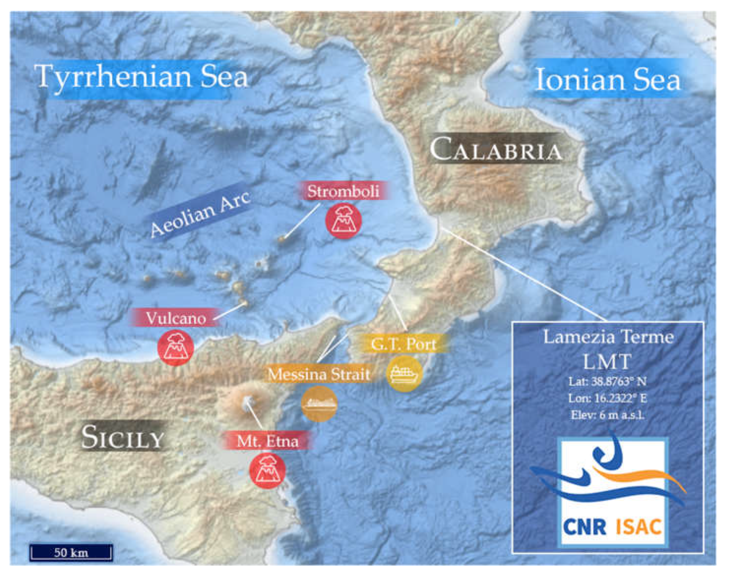
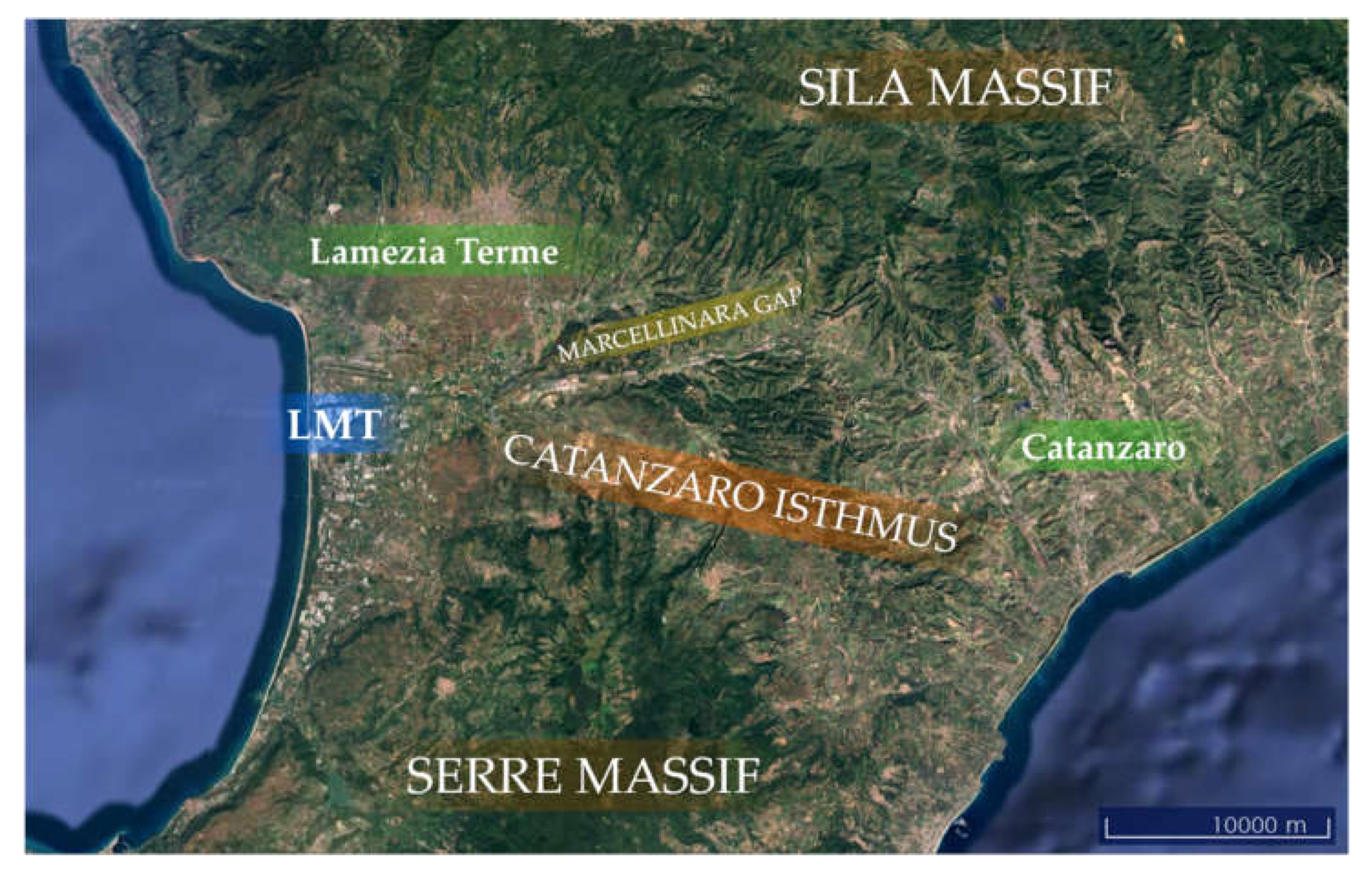
Figure 2.
Flow chart showing the steps required to calculate the Proximity Progression Factor (PPF).
Figure 2.
Flow chart showing the steps required to calculate the Proximity Progression Factor (PPF).
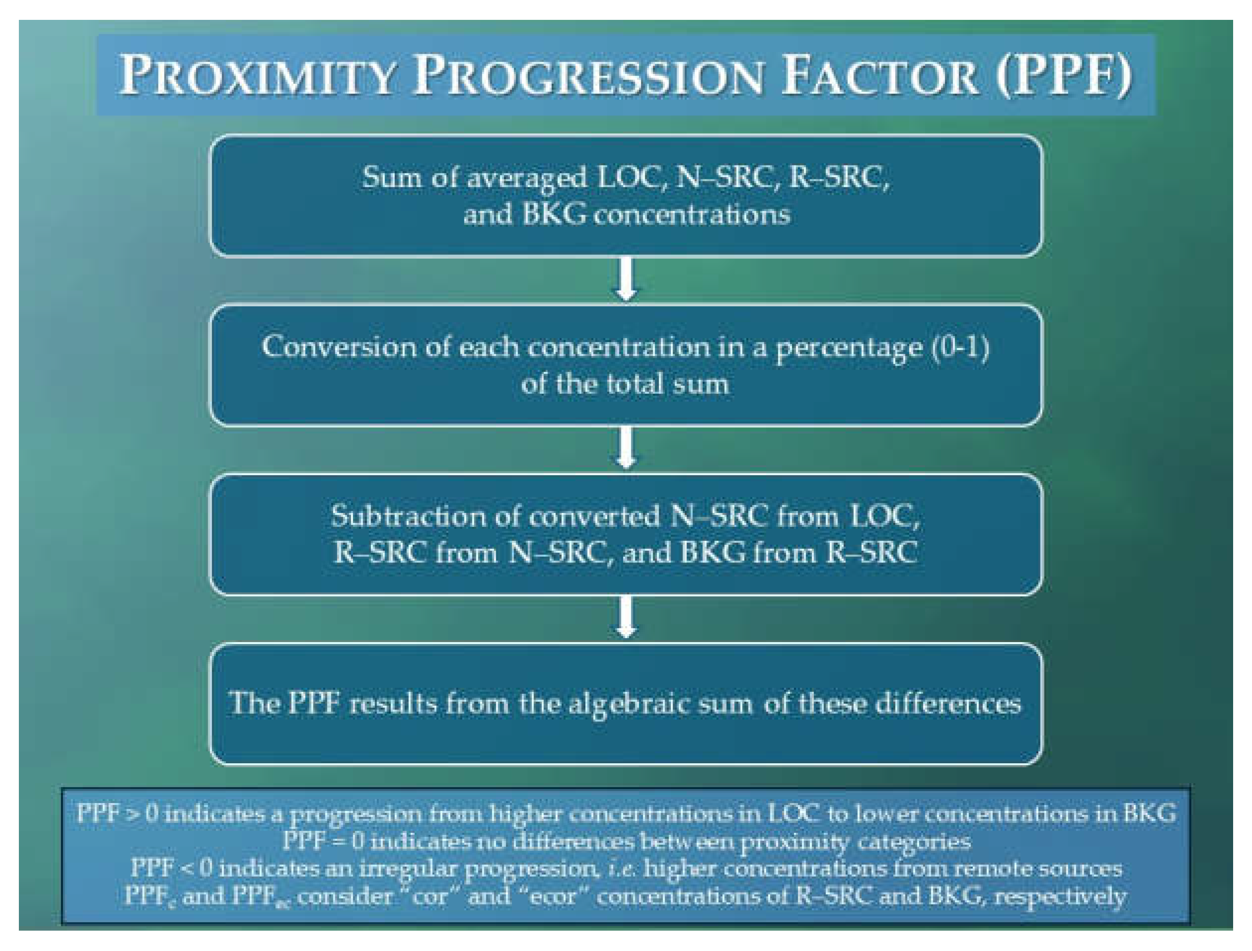
Figure 3.
Average concentrations of (A) SO2 (ppb) and (B) eBC (µg/m3) based on standard and corrected proximity categories.
Figure 3.
Average concentrations of (A) SO2 (ppb) and (B) eBC (µg/m3) based on standard and corrected proximity categories.
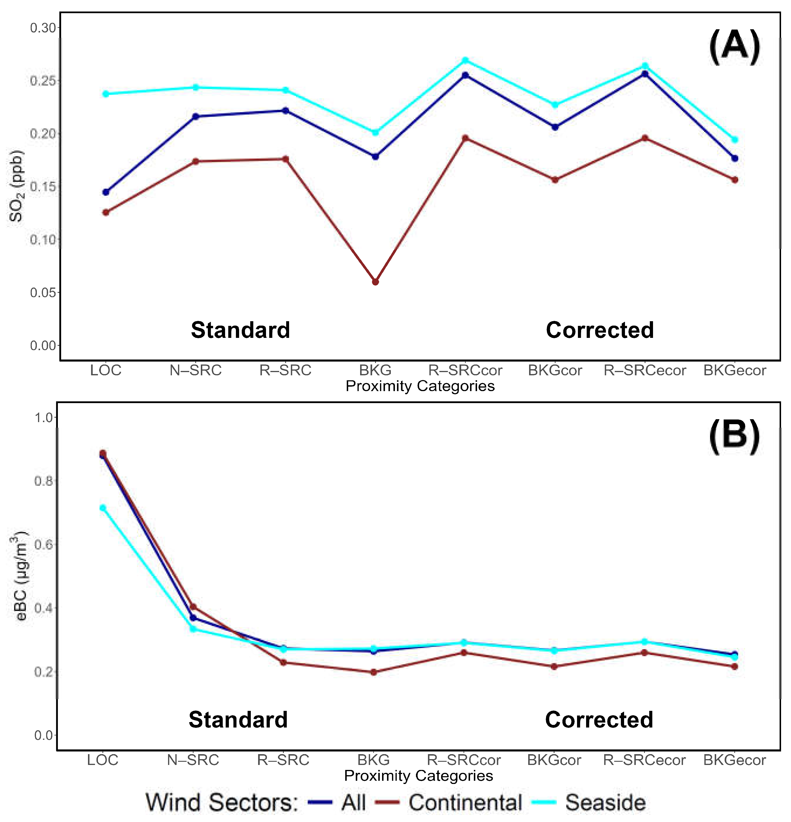
Figure 4.
Seasonal concentrations of SO2 divided by proximity category and wind sector.
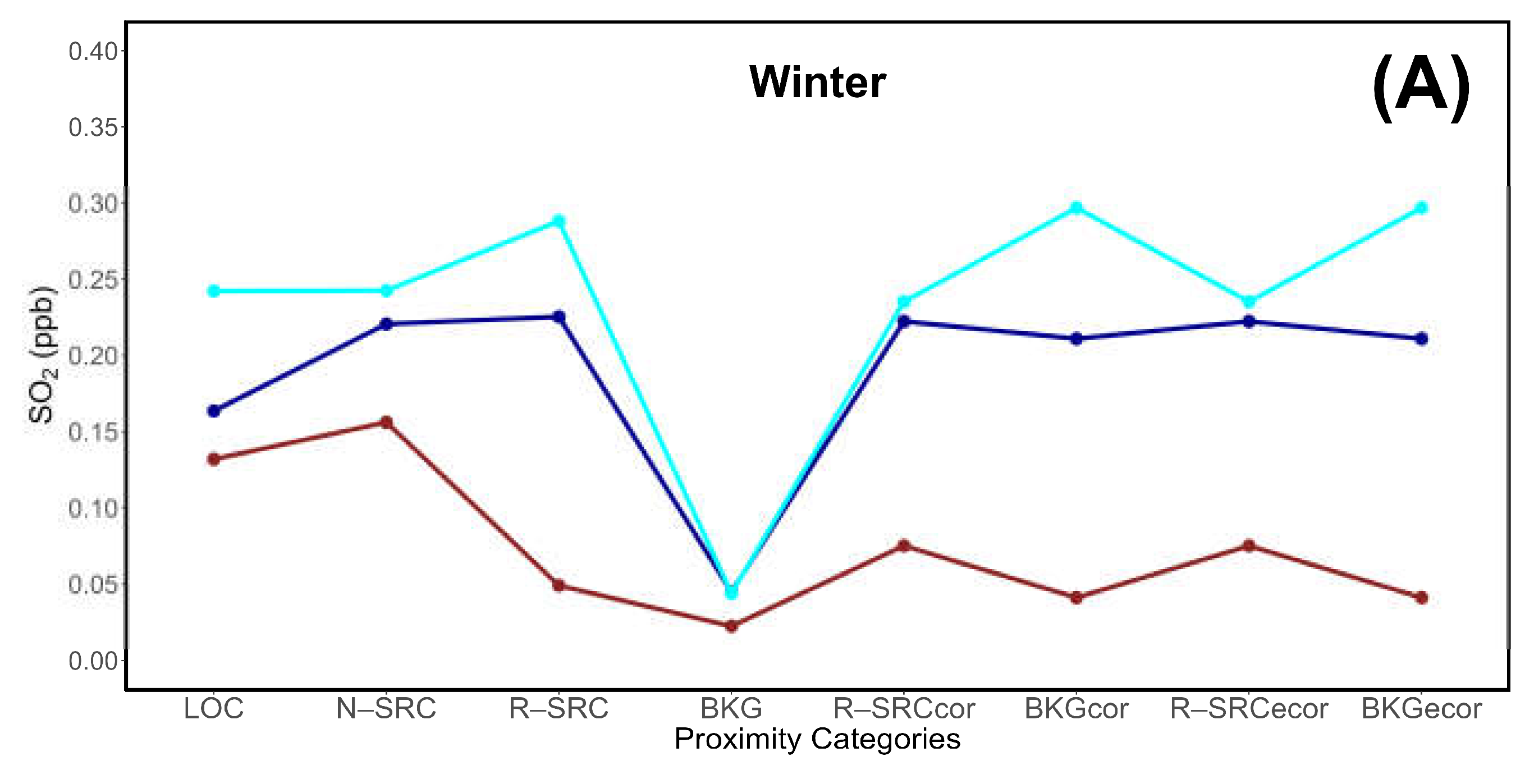
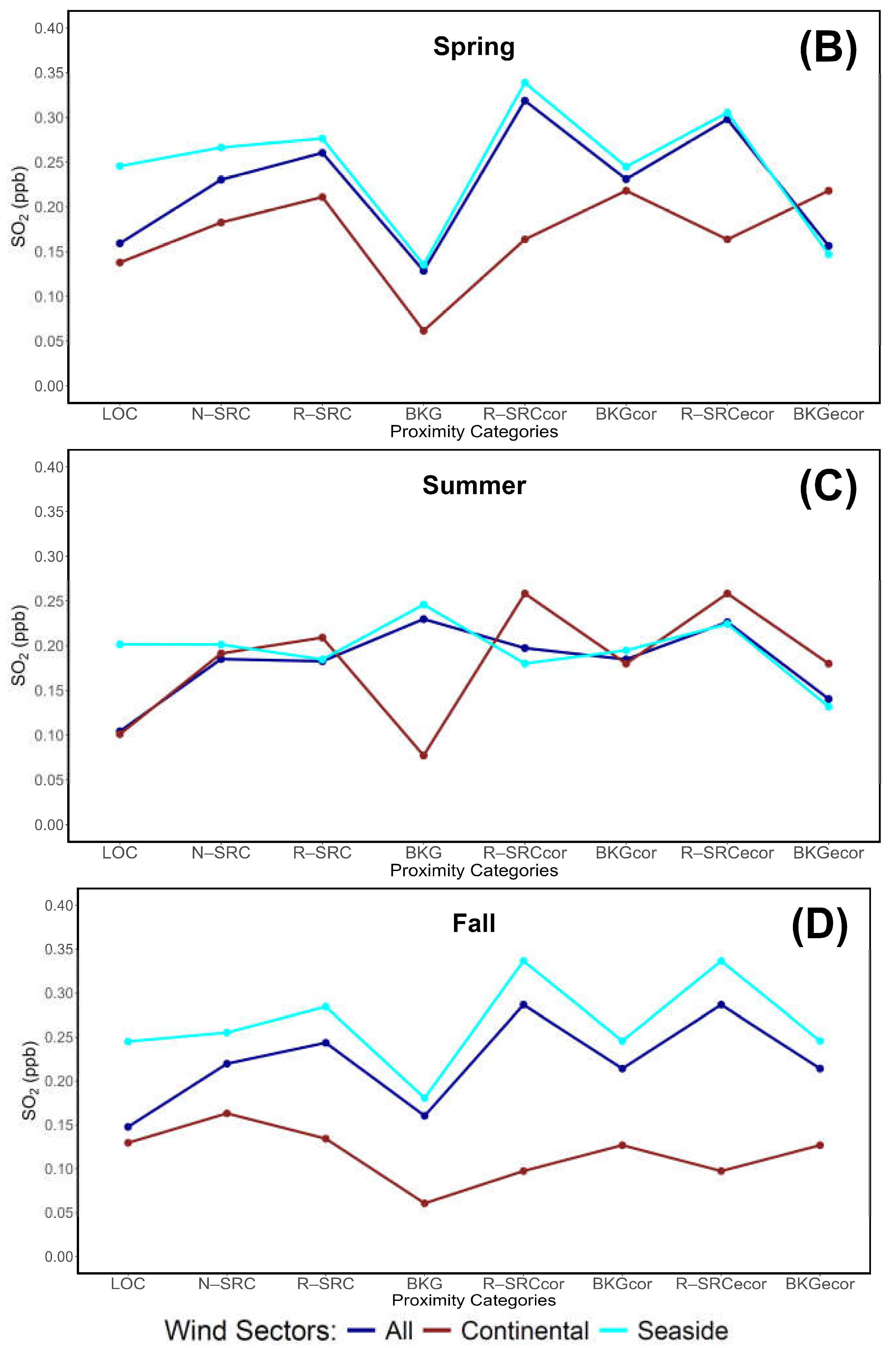
Figure 5.
Seasonal concentrations of eBC divided by proximity category and wind sector.
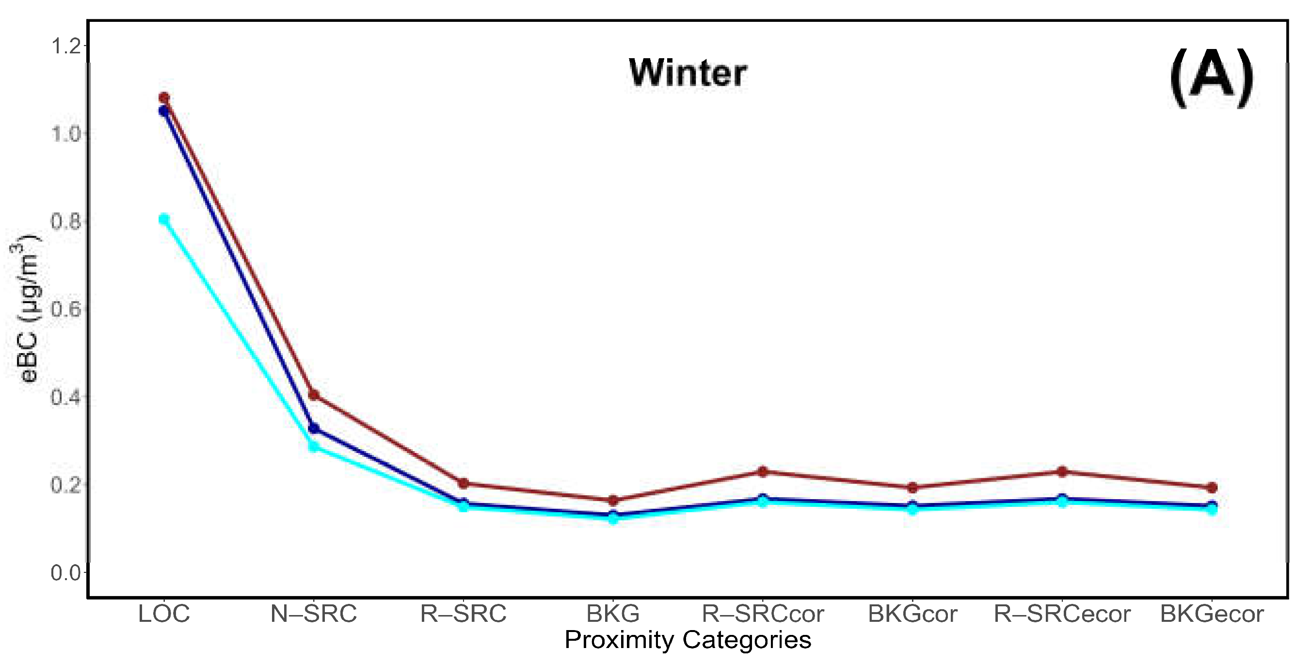
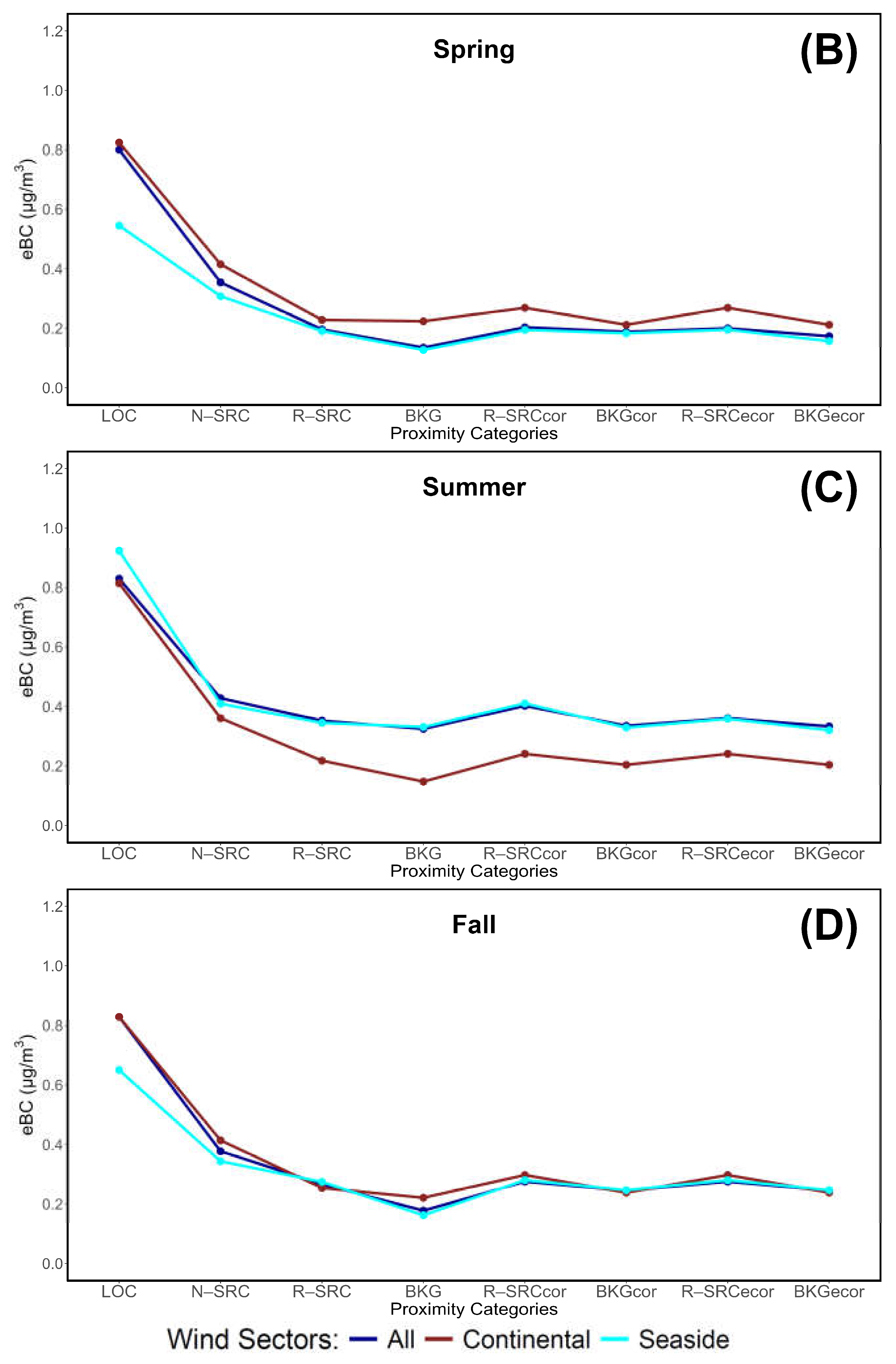
Figure 6.
Daily cycle of (A) SO2 (ppb) and (B) eBC (µg/m3) based on proximity categories. Dotted lines indicate R–SRCcor and BKGcor concentrations, while dashed lines refer to R–SRCecor and BKGecor.
Figure 6.
Daily cycle of (A) SO2 (ppb) and (B) eBC (µg/m3) based on proximity categories. Dotted lines indicate R–SRCcor and BKGcor concentrations, while dashed lines refer to R–SRCecor and BKGecor.
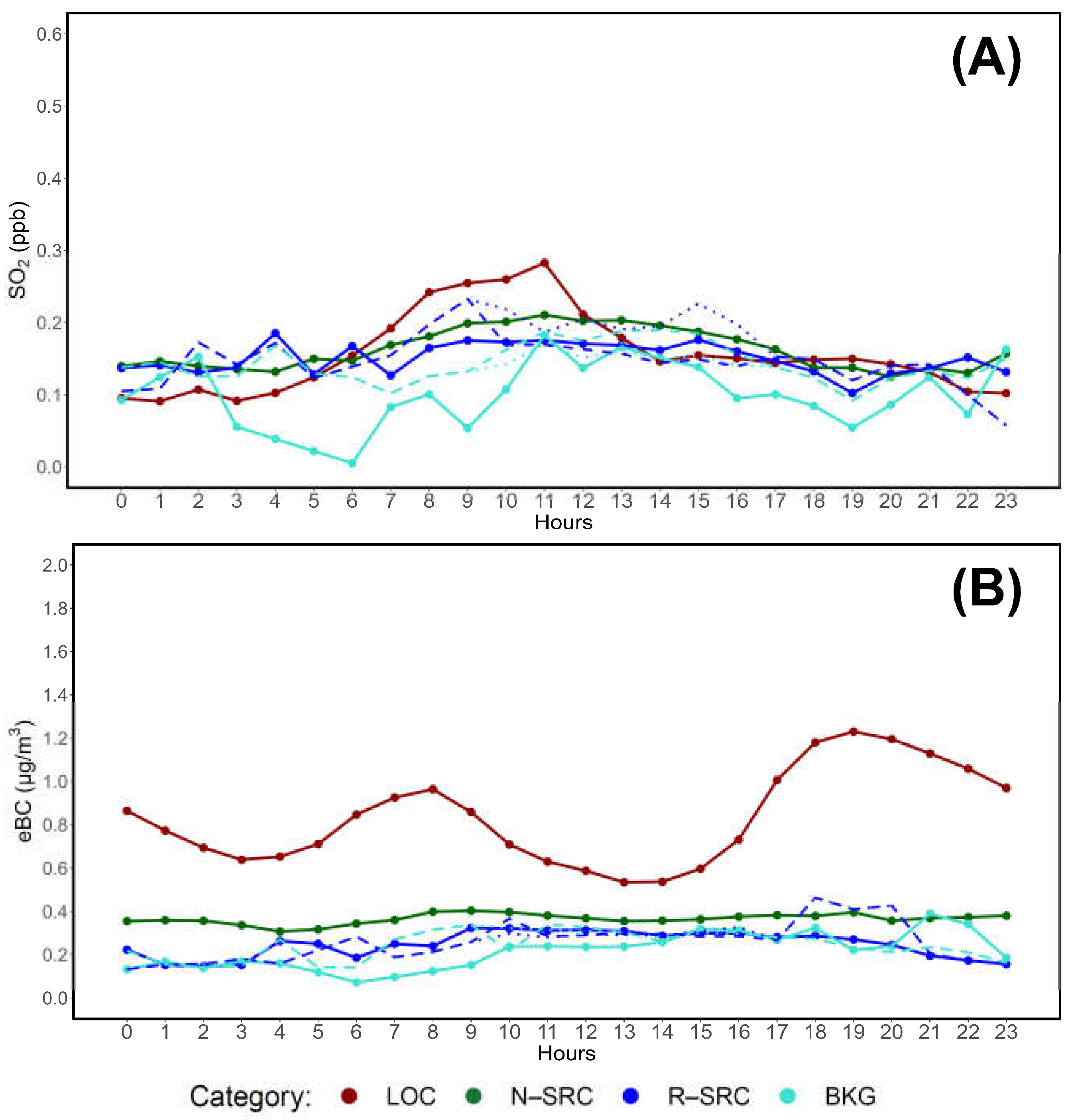
Figure 7.
Seasonal (Winter) daily cycle of (A) SO2 (ppb) and (B) eBC (µg/m3) based on proximity categories. Dotted lines indicate R–SRCcor and BKGcor concentrations.
Figure 7.
Seasonal (Winter) daily cycle of (A) SO2 (ppb) and (B) eBC (µg/m3) based on proximity categories. Dotted lines indicate R–SRCcor and BKGcor concentrations.
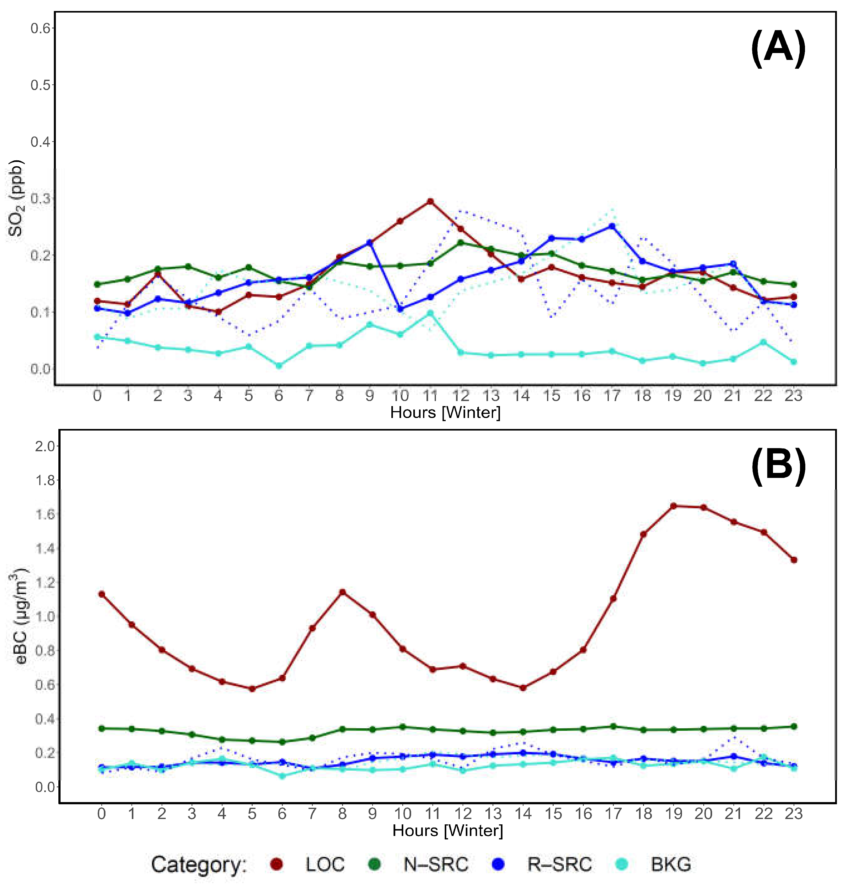
Figure 8.
Seasonal (Spring) daily cycle of (A) SO2 (ppb) and (B) eBC (µg/m3) based on proximity categories. Dotted lines indicate R–SRCcor and BKGcor concentrations, while dashed lines refer to R–SRCecor and BKGecor.
Figure 8.
Seasonal (Spring) daily cycle of (A) SO2 (ppb) and (B) eBC (µg/m3) based on proximity categories. Dotted lines indicate R–SRCcor and BKGcor concentrations, while dashed lines refer to R–SRCecor and BKGecor.
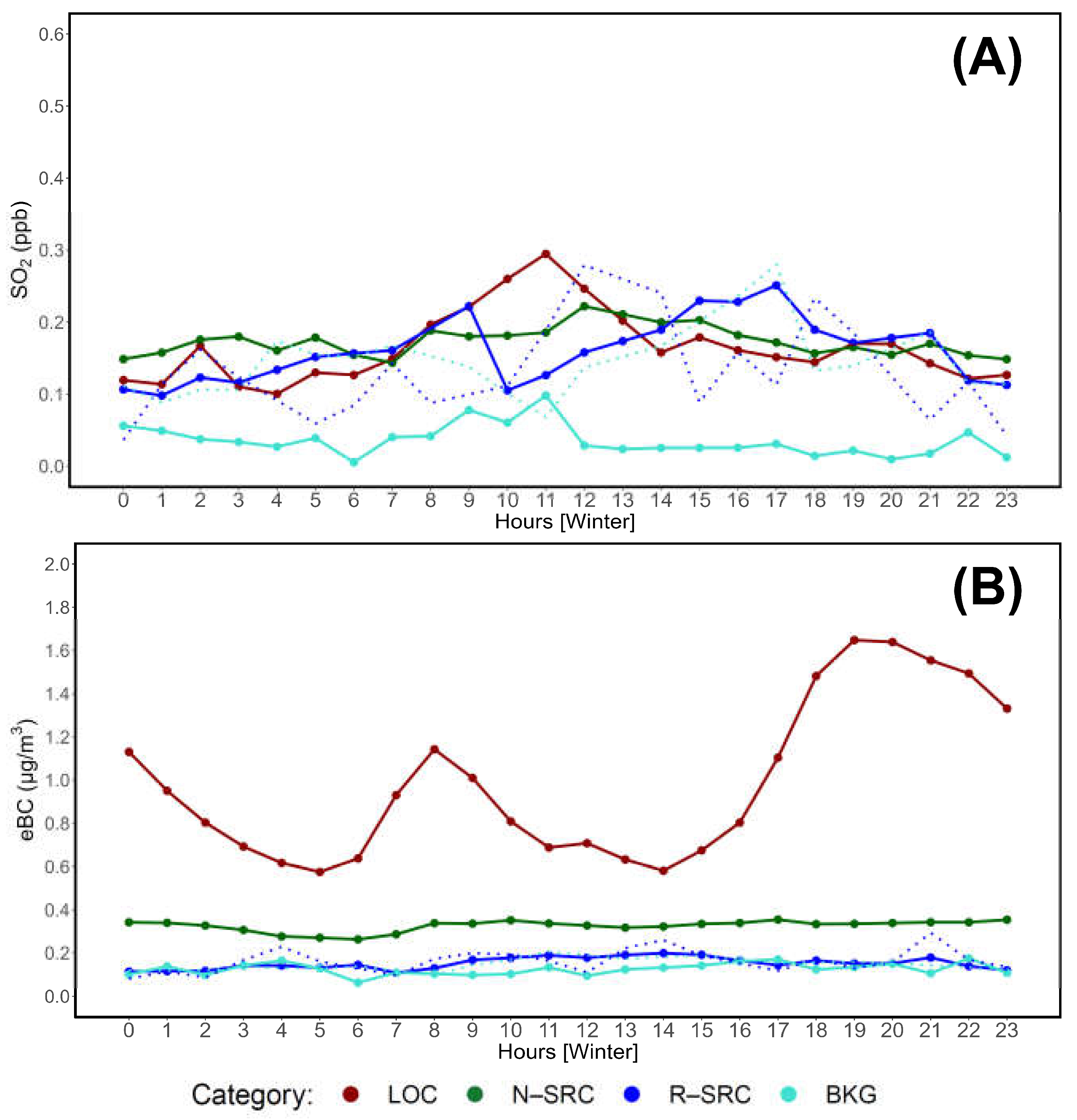
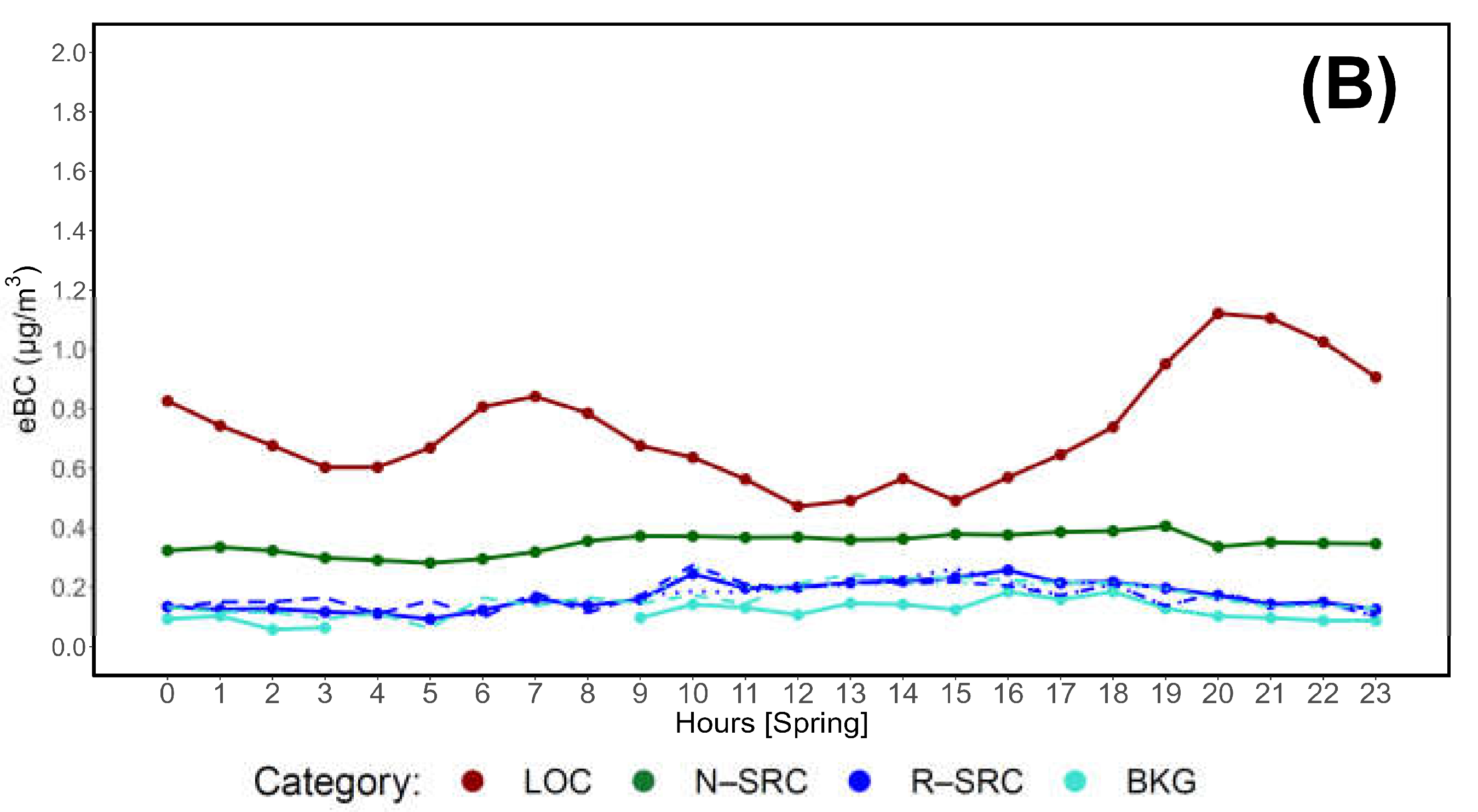
Figure 9.
Seasonal (Summer) daily cycle of (A) SO2 (ppb) and (B) eBC (µg/m3) based on proximity categories. Dotted lines indicate R–SRCcor and BKGcor concentrations, while dashed lines refer to R–SRCecor and BKGecor.
Figure 9.
Seasonal (Summer) daily cycle of (A) SO2 (ppb) and (B) eBC (µg/m3) based on proximity categories. Dotted lines indicate R–SRCcor and BKGcor concentrations, while dashed lines refer to R–SRCecor and BKGecor.
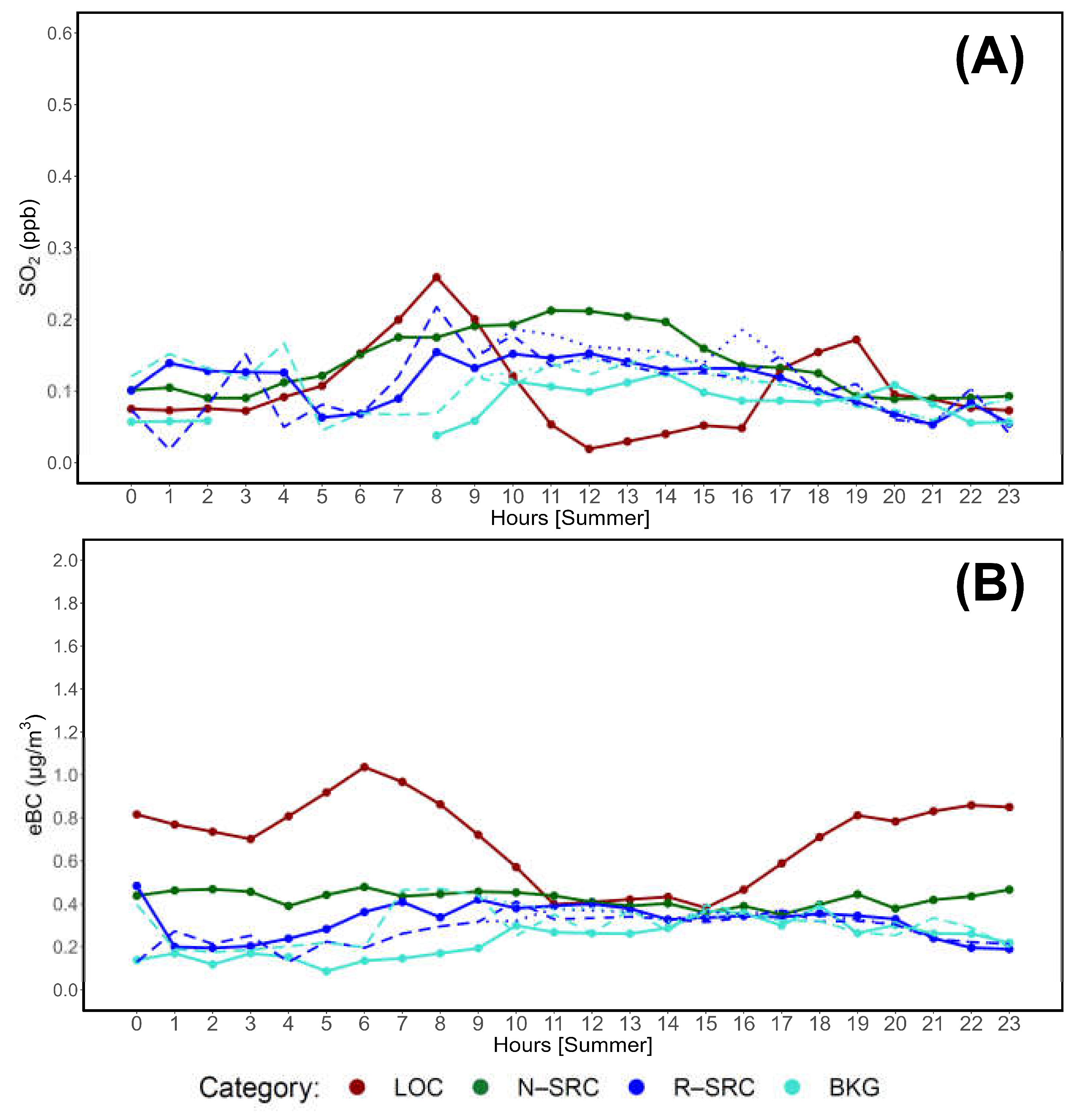
Figure 10.
Seasonal (Fall) daily cycle of (A) SO2 (ppb) and (B) eBC (µg/m3) based on proximity categories. Dotted lines indicate R–SRCcor and BKGcor concentrations.
Figure 10.
Seasonal (Fall) daily cycle of (A) SO2 (ppb) and (B) eBC (µg/m3) based on proximity categories. Dotted lines indicate R–SRCcor and BKGcor concentrations.
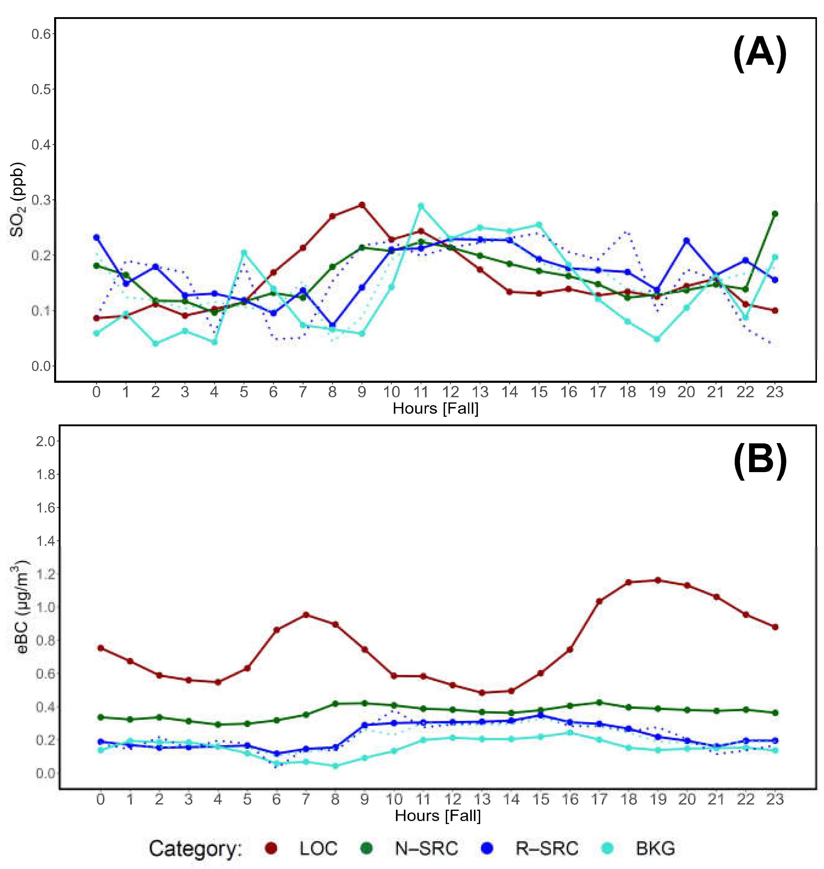
Figure 11.
Variability of SO2 (ppb) based on proximity category, wind direction, and wind speed. The radius of each polar plot refers to the concentration range of observed SO2 mole fractions.
Figure 11.
Variability of SO2 (ppb) based on proximity category, wind direction, and wind speed. The radius of each polar plot refers to the concentration range of observed SO2 mole fractions.
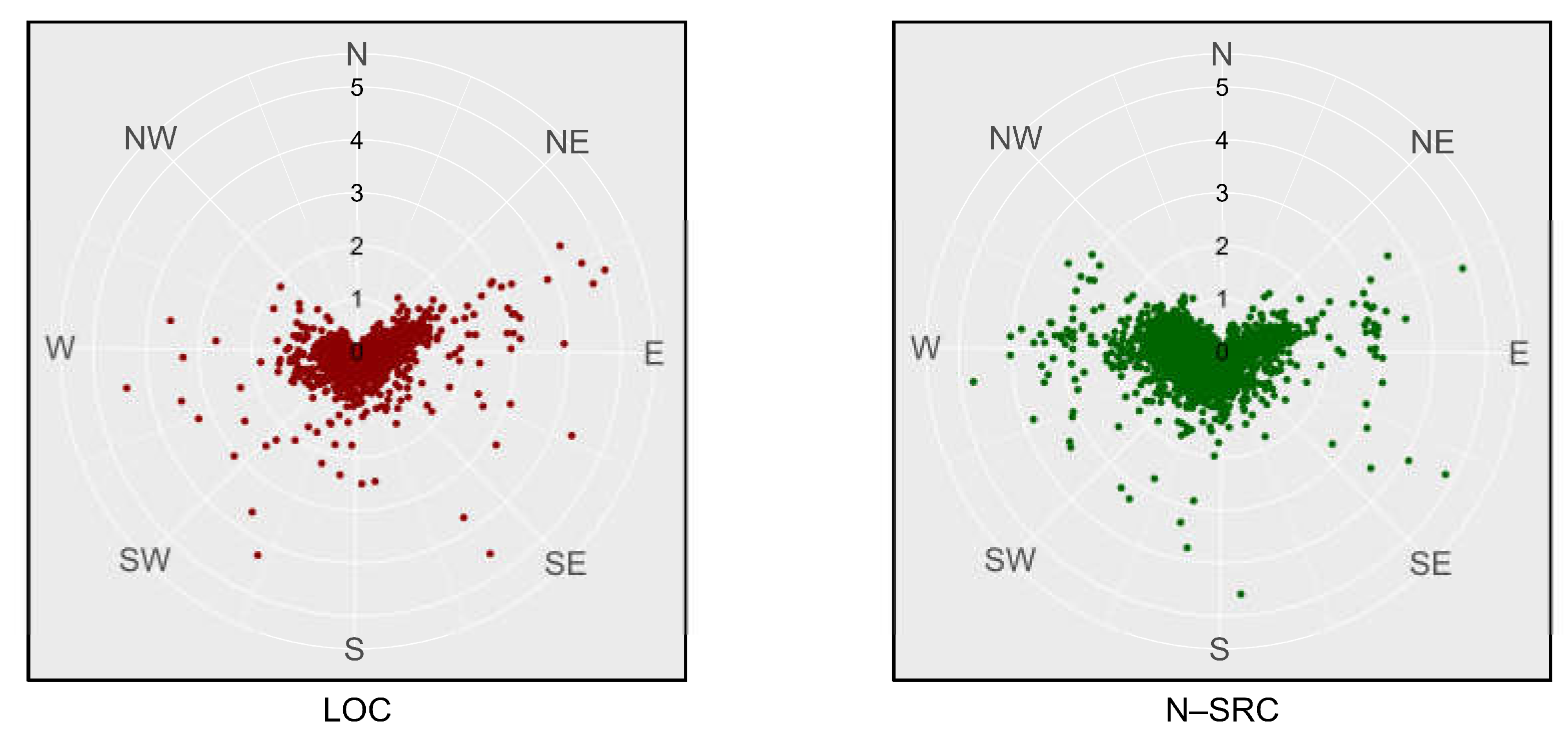
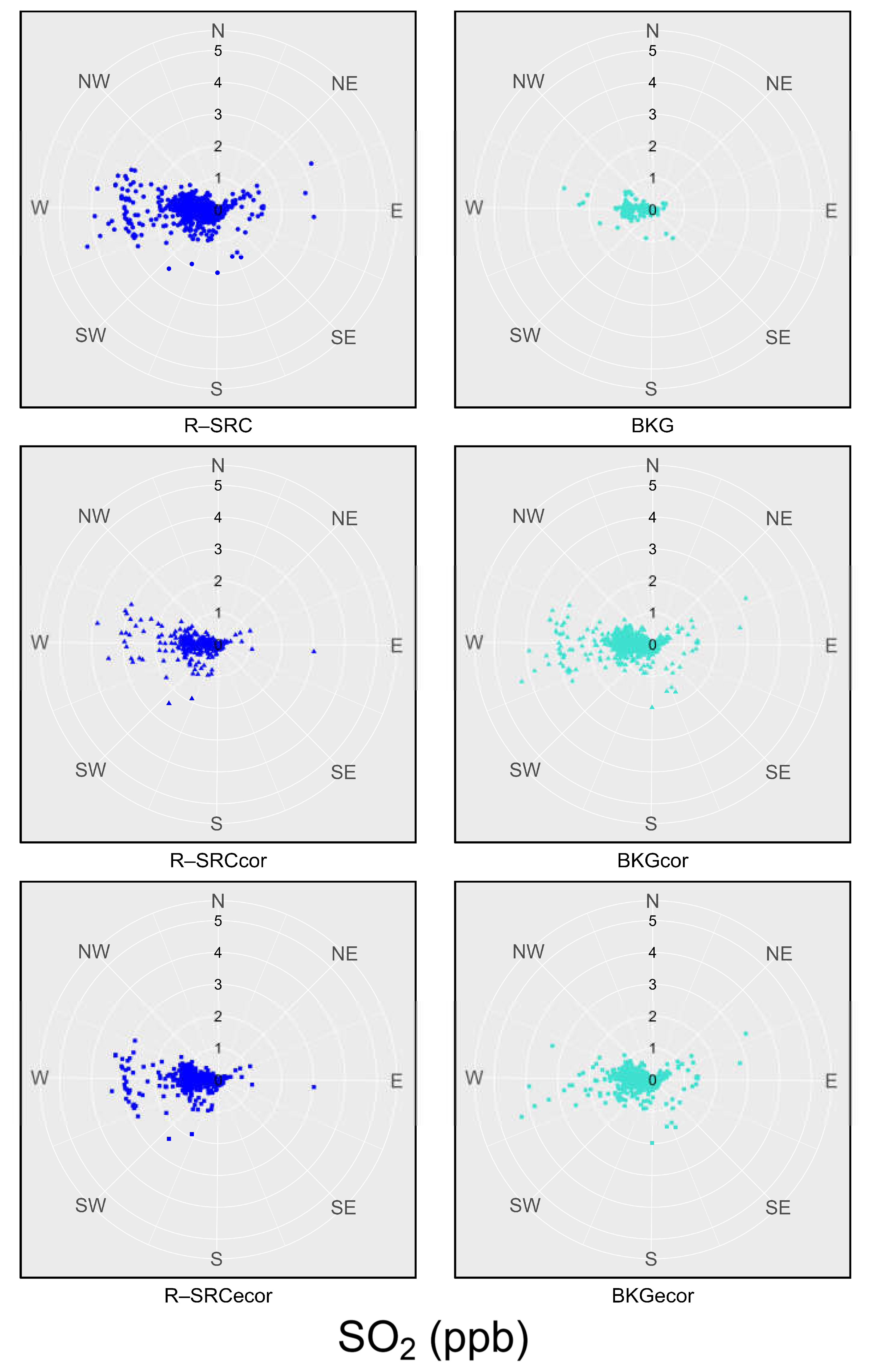
Figure 12.
Variability of eBC (µg/m3) based on proximity category, wind direction, and wind speed. The radius of each polar plot refers to the concentration range of observed eBC.
Figure 12.
Variability of eBC (µg/m3) based on proximity category, wind direction, and wind speed. The radius of each polar plot refers to the concentration range of observed eBC.
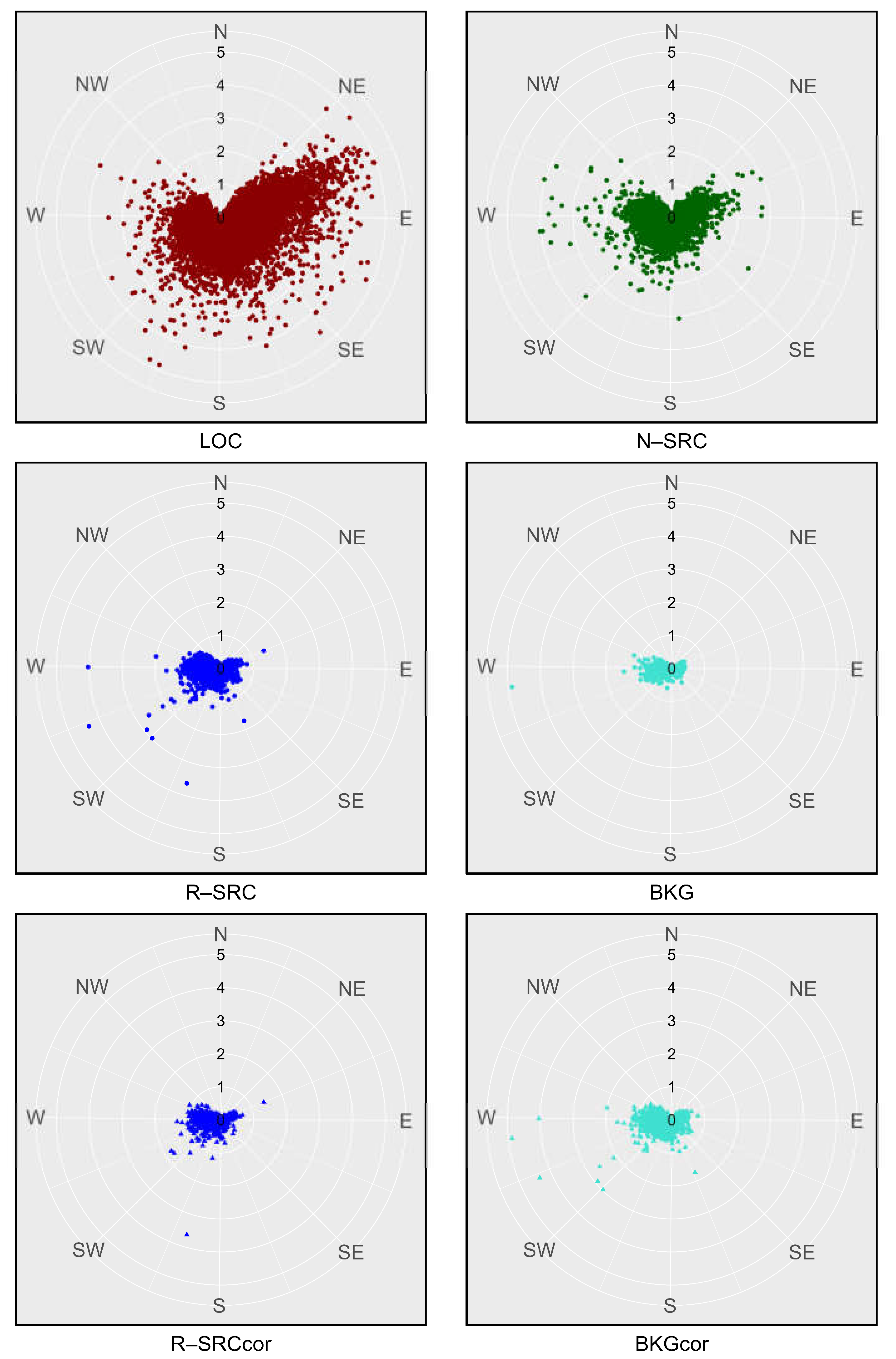
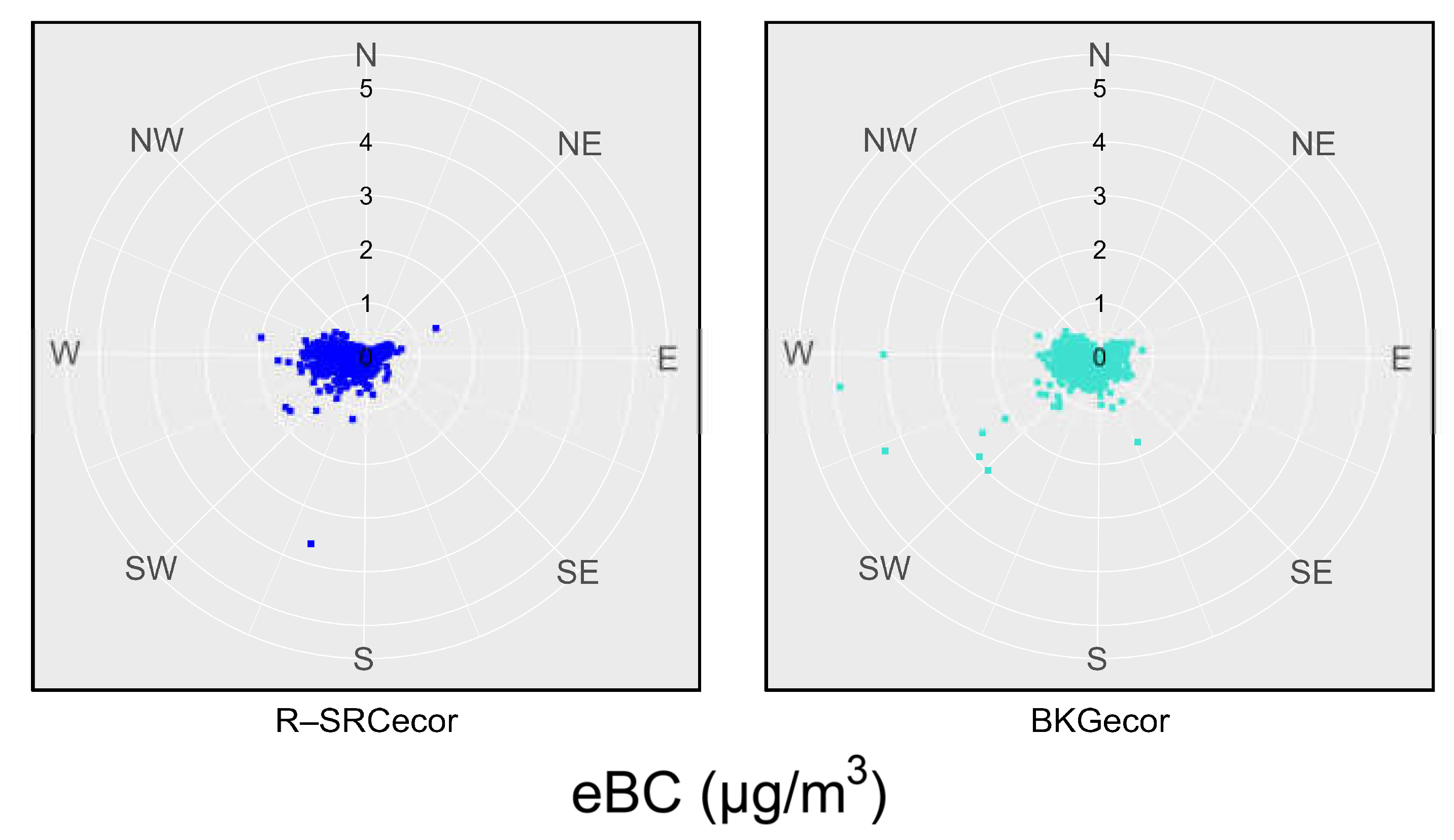
Figure 13.
Variability of SO2 (ppb) and wind speed based on proximity categories and wind corridors: western-seaside (A), northeastern-continental (B), and total (C).
Figure 13.
Variability of SO2 (ppb) and wind speed based on proximity categories and wind corridors: western-seaside (A), northeastern-continental (B), and total (C).
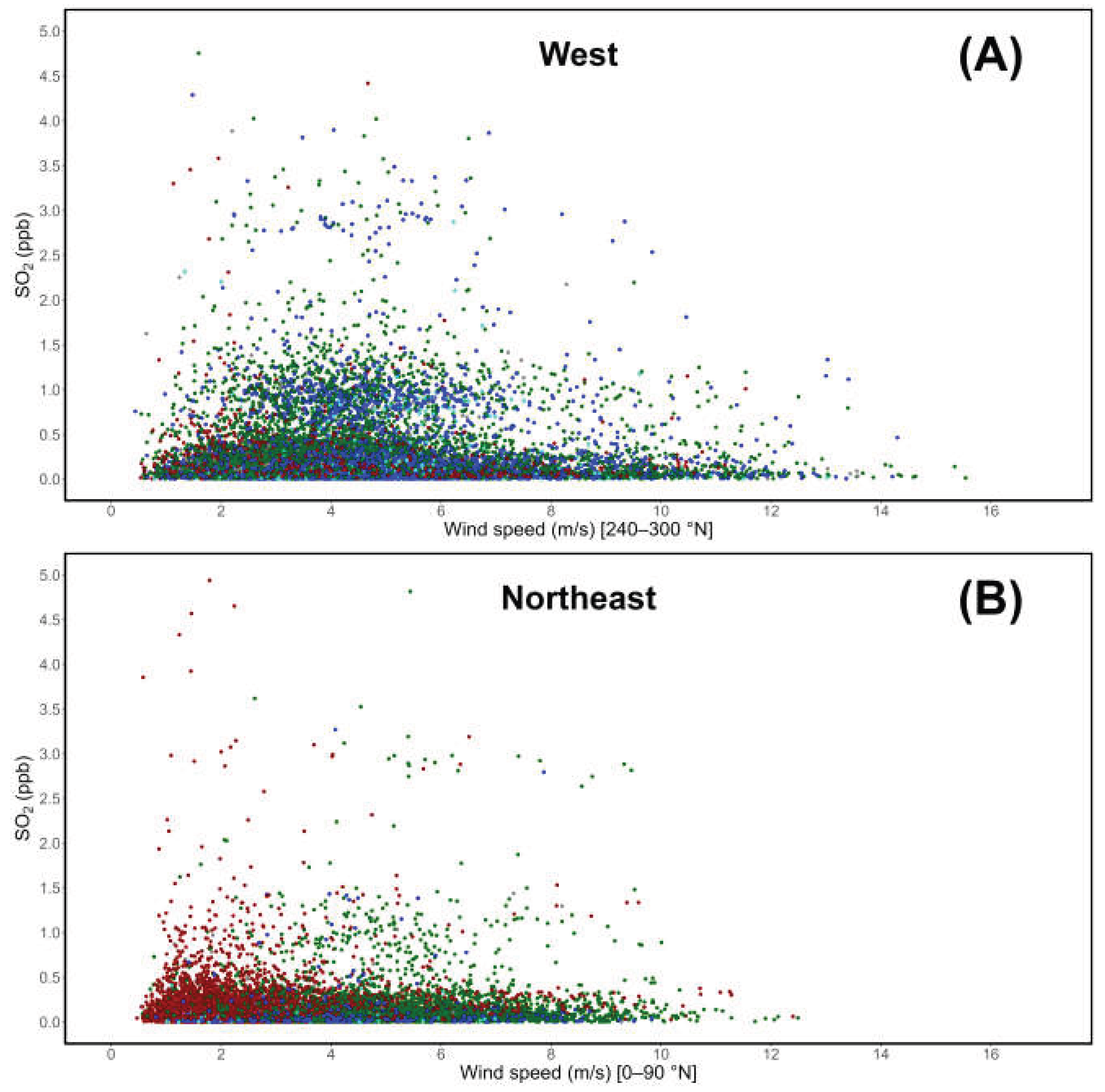
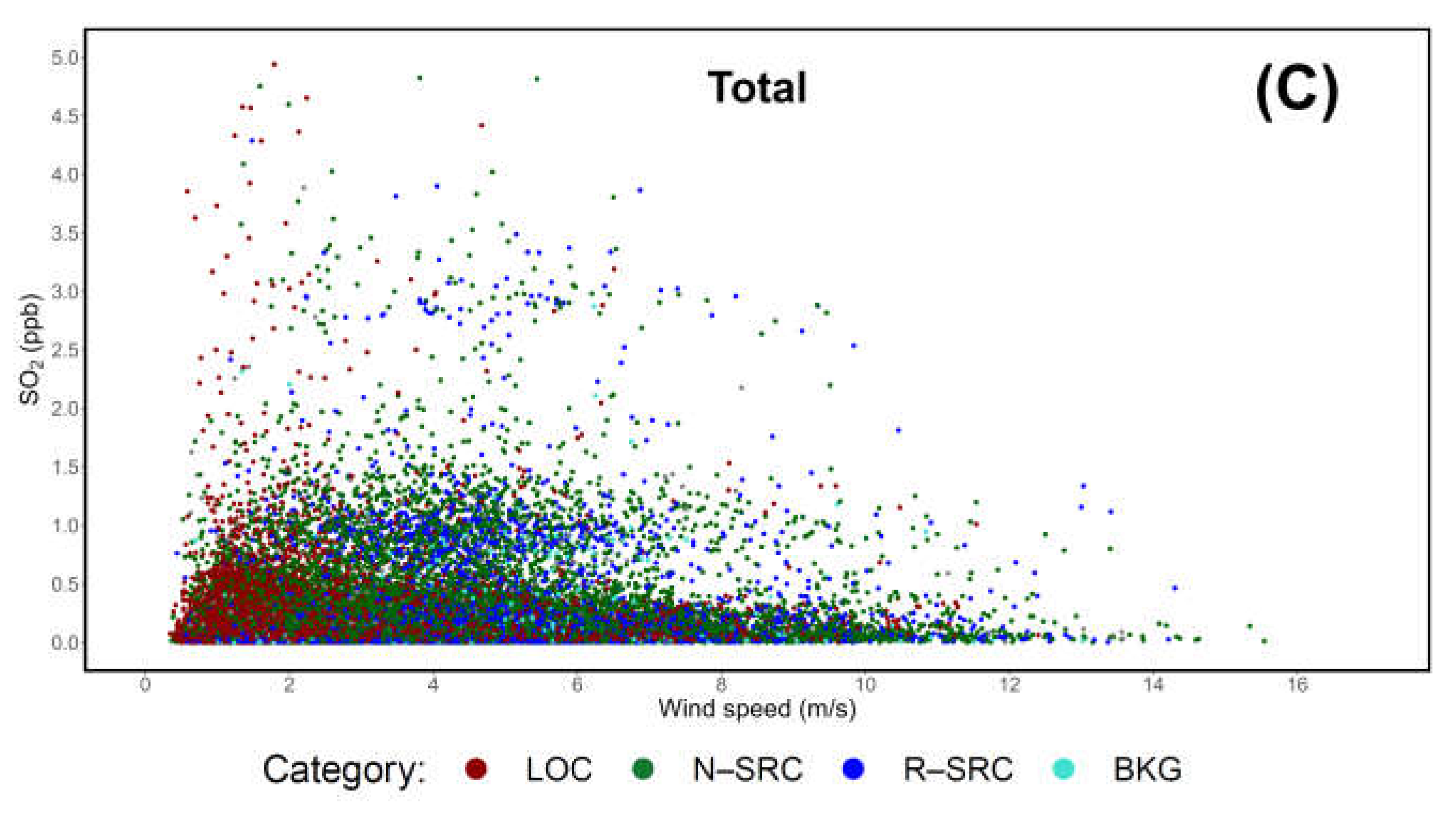
Figure 14.
Variability of eBC (µg/m3) and wind speed based on proximity categories and wind corridors: western-seaside (A), northeastern-continental (B), and total (C).
Figure 14.
Variability of eBC (µg/m3) and wind speed based on proximity categories and wind corridors: western-seaside (A), northeastern-continental (B), and total (C).
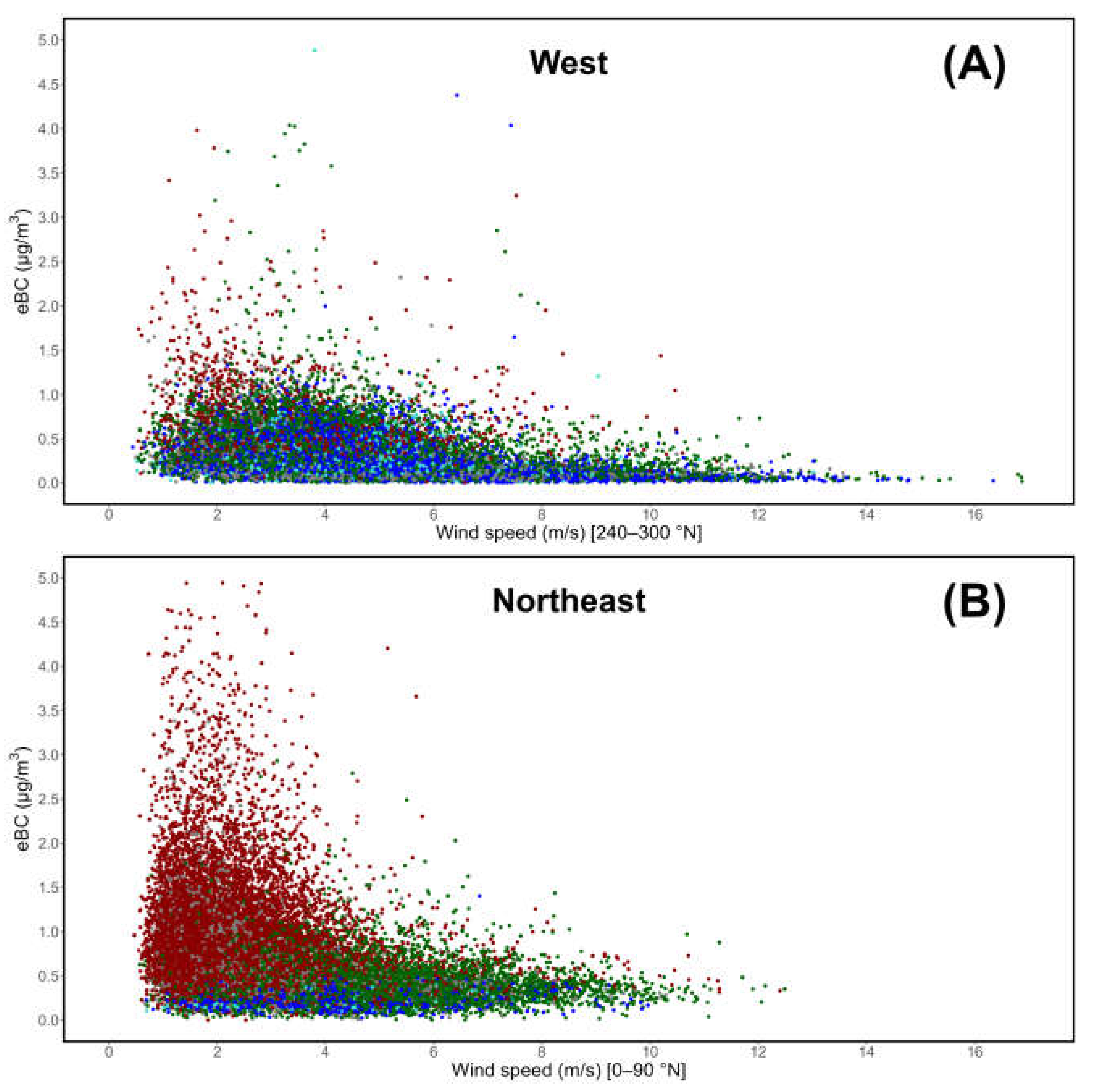
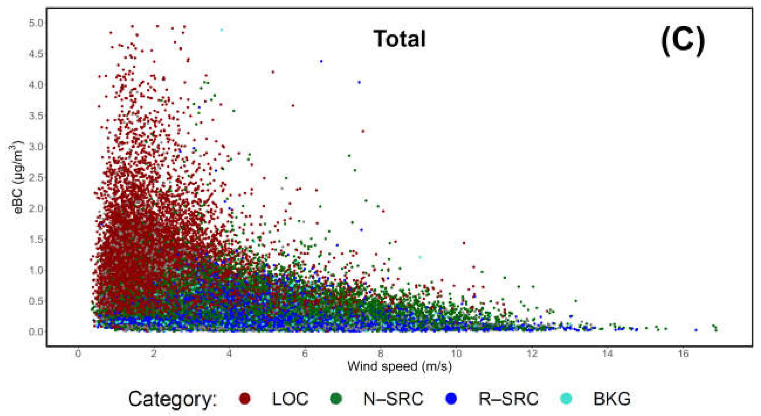
Figure 15.
Weekly cycle of SO2 (ppb) based on proximity categories and wind corridors: western-seaside (A), northeastern-continental (B), and total (C). Dotted lines indicate R–SRCcor and BKGcor concentrations, while dashed lines refer to R–SRCecor and BKGecor.
Figure 15.
Weekly cycle of SO2 (ppb) based on proximity categories and wind corridors: western-seaside (A), northeastern-continental (B), and total (C). Dotted lines indicate R–SRCcor and BKGcor concentrations, while dashed lines refer to R–SRCecor and BKGecor.
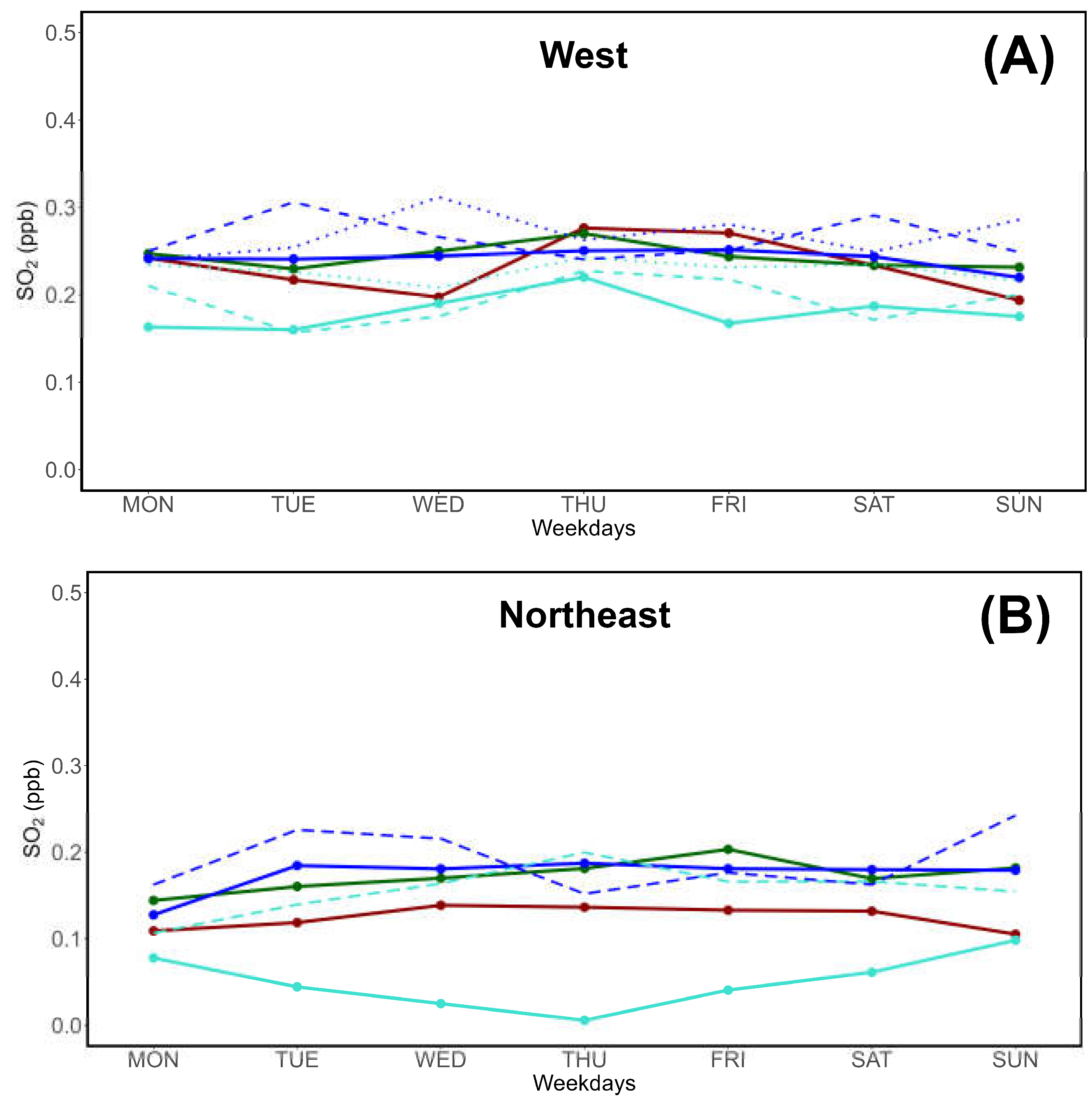
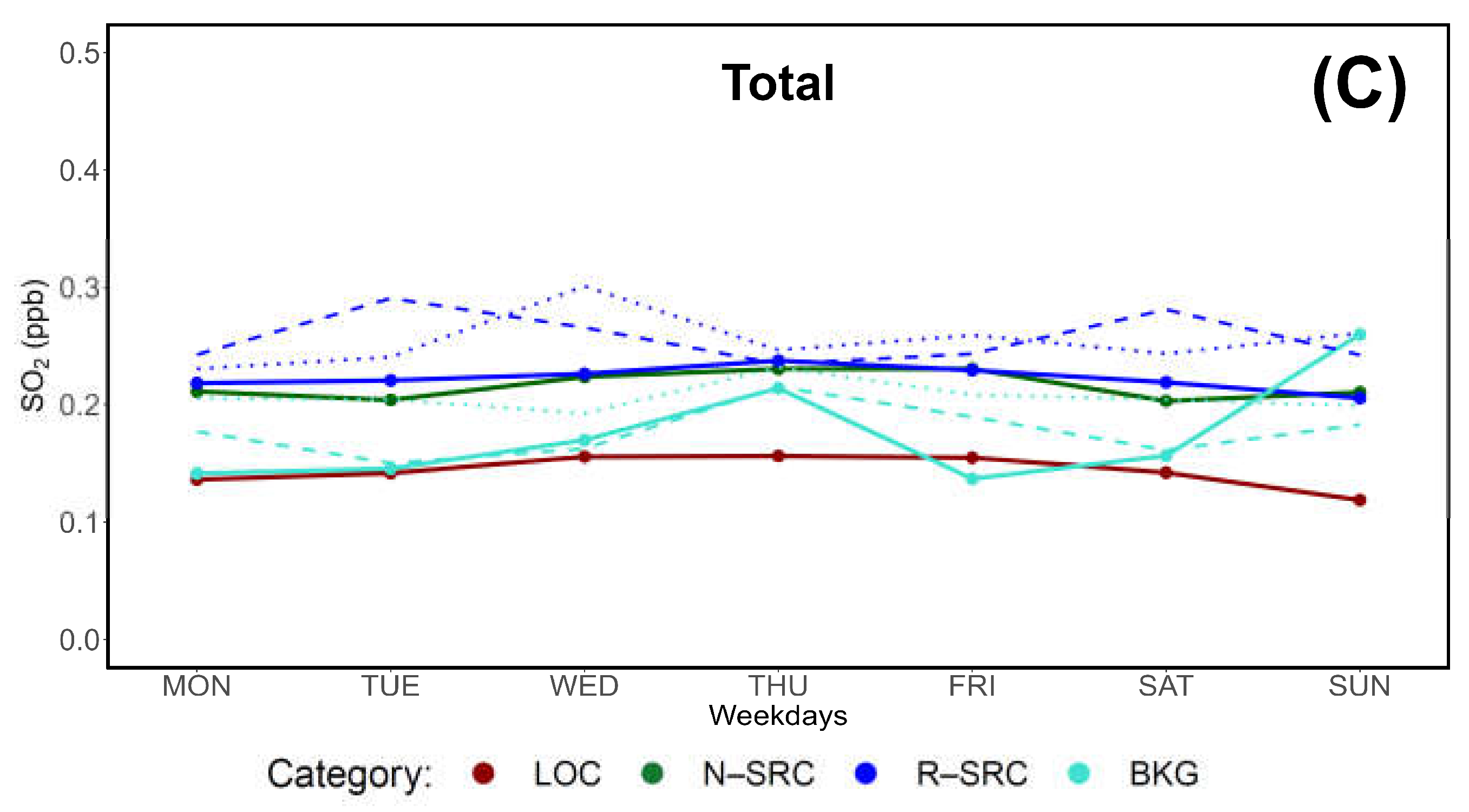
Figure 16.
Weekly cycle of eBC (µg/m3) based on proximity categories and wind corridors: western-seaside (A), northeastern-continental (B), and total (C). Dotted lines indicate R–SRCcor and BKGcor concentrations, while dashed lines refer to R–SRCecor and BKGecor.
Figure 16.
Weekly cycle of eBC (µg/m3) based on proximity categories and wind corridors: western-seaside (A), northeastern-continental (B), and total (C). Dotted lines indicate R–SRCcor and BKGcor concentrations, while dashed lines refer to R–SRCecor and BKGecor.
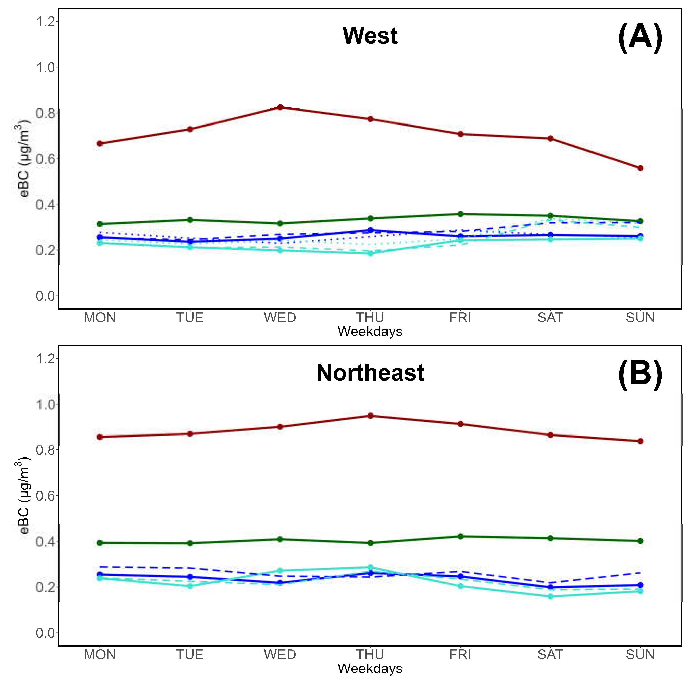
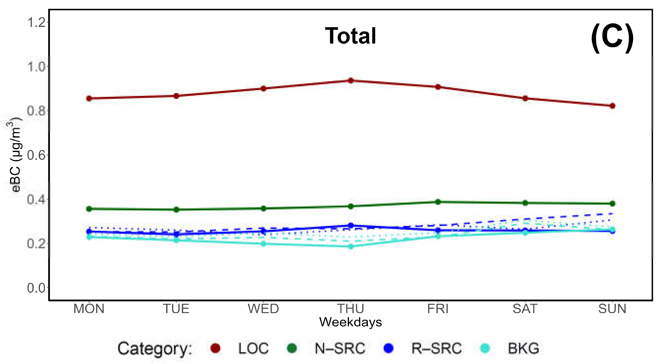
Figure 17.
Map of Southern Italy showing the approximate spatial resolution thresholds of the four main proximity categories based on SO2’s anomalous behavior and negative PPF reported in this study.
Figure 17.
Map of Southern Italy showing the approximate spatial resolution thresholds of the four main proximity categories based on SO2’s anomalous behavior and negative PPF reported in this study.
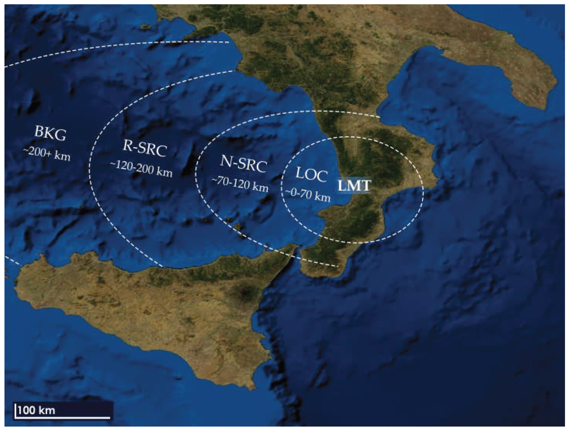

Table 1.
Coverage rates of the hourly SO2 datasets used in this study. The SMTO dataset combines Thermo Scientific 32i (SO2) and Vaisala WXT520 (meteorological parameters) measurements. SProx combines Thermo Scientific 32i measurements with hourly data for which a proximity category could be defined, i.e. valid Thermo Scientific 49i (O3) and Thermo Scientific 42i-TL (NOx) data. SMTOProx combines all previous datasets, thus resulting in lower coverage rates.
| Year | Hours | SO2 | Meteo | SMTO | SProx | SMTOProx |
| 2016 | 8784 | 63.30% | 96.34% | 62.04% | 61.28% | 60.04% |
| 2017 | 8760 | 87.76% | 93.8% | 83.86% | 86.11% | 82.23% |
| 2018 | 8760 | 97.54% | 77.05% | 75.18% | 97.04% | 74.69% |
| 2019 | 8760 | 80.67% | 98.59% | 80.65% | 77.65% | 77.63% |
| 2020 | 8784 | 34.52% | 99.98% | 34.52% | 33.03% | 33.03% |
| 2021 | 8760 | 39.08% | 99.74% | 39.07% | 35.45% | 35.44% |
| 2022 | 8760 | 65.06% | 89.85% | 63.75% | 62.48% | 61.44% |
| 2023 | 8760 | 48.59% | 96.3% | 47.37% | 48.07% | 46.86% |
| Total | 701281 | 64.56%2 | 93.95%2 | 60.80%2 | 62.63%2 | 58.92%2 |
1 Sum of all hours. 2 Average rate.
Table 2.
Coverage rates of the hourly eBC datasets used in this study. The BMTO dataset combines Thermo Scientific 5012 (eBC) and Vaisala WXT520 (meteorological parameters) measurements. BProx combines Thermo Scientific 5012 measurements with hourly data for which a proximity category could be defined, i.e. valid Thermo Scientific 49i (O3) and Thermo Scientific 42i-TL (NOx) data. BMTOProx combines all previous datasets, thus resulting in lower coverage rates.
| Year | Hours | eBC | Meteo | BMTO | BProx | BMTOProx |
| 2016 | 8784 | 93.75% | 96.34% | 93.06% | 89.70% | 89.20% |
| 2017 | 8760 | 95.27% | 93.8% | 90.45% | 92.24% | 87.93% |
| 2018 | 8760 | 95.61% | 77.05% | 73.61% | 94.44% | 72.5% |
| 2019 | 8760 | 96.48% | 98.59% | 96.46% | 92.26% | 92.23% |
| 2020 | 8784 | 96.61% | 99.98% | 96.60% | 91.75% | 91.74% |
| 2021 | 8760 | 98.42% | 99.74% | 98.25% | 77.39% | 77.38% |
| 2022 | 8760 | 97.43% | 89.85% | 88% | 67.37% | 65.98% |
| 2023 | 8760 | 69.13% | 96.3% | 68.81% | 60.51% | 60.19% |
| Total | 701281 | 92.83%2 | 93.95%2 | 88.15%2 | 83.20%2 | 79.64%2 |
1 Sum of all hours. 2 Average rate.
Table 3.
Concentrations of SO2 (ppb) and eBC (µg/m3) on a per-category basis, also including the ±1σ interval (one standard deviation). Data are divided by wind sector.
Table 3.
Concentrations of SO2 (ppb) and eBC (µg/m3) on a per-category basis, also including the ±1σ interval (one standard deviation). Data are divided by wind sector.
| Category | SO2 (ppb) | eBC (µg/m3) | ||||
| All | Nor. East | West | All | Nor. East | West | |
| LOC | 0.145 ± 0.280 |
0.125 ± 0.257 |
0.237 ± 0.399 |
0.879 ± 0.632 |
0.887 ± 0.644 |
0.715 ± 0.517 |
| N–SRC | 0.216 ± 0.357 |
0.174 ± 0.319 |
0.243 ± 0.381 |
0.369 ± 0.341 |
0.404 ± 0.245 |
0.334 ± 0.295 |
| R–SRC | 0.222 ± 0.402 |
0.176 ± 0.351 |
0.241 ± 0.424 |
0.273 ± 0.605 |
0.229 ± 0.119 |
0.270 ± 0.581 |
| BKG | 0.178 ± 0.309 |
0.060 ± 0.083 |
0.201 ± 0.334 |
0.264 ± 0.788 |
0.198 ± 0.089 |
0.272 ± 0.846 |
| R–SRCcor | 0.255 ± 0.449 |
0.196 ± 0.365 |
0.269 ± 0.465 |
0.291 ± 0.730 |
0.259 ± 0.130 |
0.290 ± 0.785 |
| BKGcor | 0.206 ± 0.376 |
0.156 ± 0.329 |
0.227 ± 0.400 |
0.266 ± 0.611 |
0.216 ± 0.111 |
0.265 ± 0.590 |
| R–SRCecor | 0.256 ± 0.432 |
0.196 ± 0.365 |
0.264 ± 0.438 |
0.294 ± 0.637 |
0.259 ± 0.130 |
0.294 ± 0.653 |
| BKGecor | 0.176 ± 0.323 |
0.156 ± 0.329 |
0.194 ± 0.340 |
0.253 ± 0.657 |
0.216 ± 0.111 |
0.245 ± 0.649 |
Table 4.
Proximity Progression Factor (PPF) of SO2 and eBC, from this study, compared with the PPF of CO, CO2, and CH4 based on the findings of previous research on concentration variability by air mass aging category. PPFc and PPFec consider “cor” and “ecor” corrections of R–SRC (remote source) and BKG (atmospheric background) categories.
| Parameter | PPF | PPFc | PPFec |
| SO2 | -0.043 | -0.074 | -0.039 |
| eBC | 0.345 | 0.340 | 0.349 |
| CO | 0.130 | 0.123 | 0.124 |
| CO2 | 0.024 | 0.022 | 0.022 |
| CH4 | 0.024 | 0.023 | 0.023 |
Disclaimer/Publisher’s Note: The statements, opinions and data contained in all publications are solely those of the individual author(s) and contributor(s) and not of MDPI and/or the editor(s). MDPI and/or the editor(s) disclaim responsibility for any injury to people or property resulting from any ideas, methods, instructions or products referred to in the content. |
© 2025 by the authors. Licensee MDPI, Basel, Switzerland. This article is an open access article distributed under the terms and conditions of the Creative Commons Attribution (CC BY) license (http://creativecommons.org/licenses/by/4.0/).
Copyright: This open access article is published under a Creative Commons CC BY 4.0 license, which permit the free download, distribution, and reuse, provided that the author and preprint are cited in any reuse.


