
Submitted:
28 October 2024
Posted:
30 October 2024
You are already at the latest version
Abstract
In this paper, we analyzed the influence of spin Nernst effect on quantum correlation in the layered ferrimagnetic model. In the study of three-dimensional ferrimagnets, the focus is on materials with a specific arrangement of spins, where neighboring spins are parallel and other antiparallel. The anisotropic nature of these materials means that the interactions between spins depend on their relative orientations in different directions. We analyzed the effect of magnon bands induced by the coupling parameters on entanglement negativity. The influence of the coupling parameters of the topologic phase transition on quantum entanglement is investigated as well. Numerical simulations using Lanczos algorithm and exact diagonalization for different sizes lattice are compared with the results of the spin wave theory.
Keywords:
entanglement negativity
; spin Nernst coefficient
; exact diagonalization
1. Introduction
Quantum correlation in low-dimensional magnets is an important topic in recent years which connects quantum information theory and condensed matter physics [1,2,3]. In the context of quantum spin systems, quantum correlation refers to the entanglement and non-classical correlations that exist between quantum particles. In three-dimensional ferrimagnets or layered ferrimagnets, the interplay between topological phase transitions and quantum correlations give rise to a range of intriguing phenomena, where entanglement plays a crucial role in determining of ground state properties, and various other spin exotic phenomena observed in ferrimagnetic systems [1,2,3,4,5,6,7,8,9,10,11,12,13,14,15,16,17,18,19]. On the other hand, the spin Nernst effect refers to the generation of an electric field perpendicular to both an applied temperature gradient and external field. It is an important phenomenon that occurs in materials with broken time-reversal symmetry, being a variant of the standard Nernst effect, where the generated electric field is proportional to the spin current rather than the charge current. In the framework of layered ferrimagnets, it may emerges in the system due to the interplay between temperature gradients, magnetic fields, and spin transport. In general, when a temperature gradient is applied through a ferrimagnet, it may induce a spin current perpendicular to the temperature gradient, resulting in a transverse voltage known as spin Nernst voltage. This effect is directly related to the magnon Hall effect and can provide insights into the spin dynamics of ferrimagnetic materials. To study quantum correlations and spin Nernst effect in a layered ferrimagnet, several theoretical models and computational techniques are employed such as spin wave theory, density matrix renormalization group, quantum Monte Carlo exact diagonalization. Being the predictions regarding quantum entanglement and spin Nernst effect depend on the specific model, Hamiltonian, and parameters used in the study. The goal is to explore these phenomena experimentally and theoretically to gain a deeper understanding of the behavior of quantum spins in magnetic materials. In the layered ferrimagnet, the influence of magnon bands on quantum correlation is an interesting aspect to explore. The Heisenberg model describes the system with anisotropic and isotropic interactions being a widely studied model for understanding of the behavior of layered ferrimagnets. In general, quantum correlations and entanglement in the Heisenberg model can be quantified using differents quantifiers as von Neumann entanglement entropy or entanglement spectrum. The von Neumann entropy provides information about the degree of entanglement between different regions of the spin system. The entanglement spectrum, on the other hand, gives insights into the energy levels associated with the entanglement.
The presence of anisotropic interactions introduces a characteristic anisotropy in the magnon dispersion which affects the entanglement dynamics, where the magnon bands determine the spectrum of magnons, which, in turn, affect the entanglement dynamics. The von Neumann entropy and spectrum may exhibit different behaviors depending on the specific features of the magnon bands, such as their bandwidth, dispersion relation, and anisotropy. For example, the presence of gapless magnon modes can lead to long-range entanglement and power-law scaling of the von Neumann entropy. On the other hand, the presence of a magnon gap can suppress entanglement and lead to short-range correlations. The study of magnon bands and their influence on entanglement in the ferromagnetic and antiferromagnetic Heisenberg model often involves theoretical approaches such as spin wave theory, bosonization techniques, or numerical methods like exact diagonalization, which provide insights into the entanglement properties and their connection to the magnon spectrum of the system. Thus, the understanding of the interplay of magnon bands and entanglement is crucial for unraveling of quantum nature of ferrimagnetic systems. Helping in characterizing of ground state properties, and exploring the emergence of novel phenomena in these systems [20].
The goal of this paper is to analyze the influence of variation of the spin Nernst coefficient with coupling parameters on entanglement negativity. The paper is organized as follows: in Section 2, we discuss about the three-dimensional layered ferrimagnet and theirs properties. In Section 3, we present our analytical and numerical, where we discuss the variation of the spin Nernst conductivity and the behavior of the entanglement negativity as a function of T. In the last Section 4, we present our conclusions.
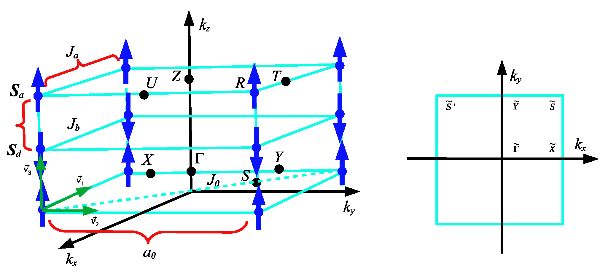
Figure 1.
Lattice model for a layered ferrimagnet with ferromagnetic layers along z axis. is the inter-layer coupling, and indicate the exchange interactions between nearest-neighbors. The red arrows are the basis vectors, defined as . and , with being the in-plane lattice spacing.
Figure 1.
Lattice model for a layered ferrimagnet with ferromagnetic layers along z axis. is the inter-layer coupling, and indicate the exchange interactions between nearest-neighbors. The red arrows are the basis vectors, defined as . and , with being the in-plane lattice spacing.
2. Model
General Hamiltonian for the layered ferrimagnet: For a layered ferrimagnet system with two types of ferromagnetic sublayers a and d sublattices stacked periodically, we consider the Hamiltonian with intralayer ferromagnetic exchange interactions for each sublattice; interlayer antiferromagnetic coupling between adjacent sublayers; magnetic anisotropy for each sublattice; external magnetic field applied to the system and dipole-dipole interaction as a perturbation to account for long-range dipolar effects. The model is composed by:
Antiferromagnetic interlayer exchange coupling between neighboring layers:
Magnetic anisotropy for each sublattice:
External magnetic field:
Dipole-dipole interaction (perturbative term):
where is the unit vector between spins i and j and is the distance between them. is the external magnetic field vector. Thus, the total Hamiltonian for the system is:
The model captures the interactions within and between the two sublattices as well as the influence of anisotropy, external fields and long-range dipolar effects.
3. Results
Entanglement is a quantum mechanical property that Schrödinger singled out as "the characteristic trait of quantum mechanics" and that has been many analyzed in connection with Bell’s inequality [25,26,27,28,29,30,31,32]. In general, a pure pair of quantum systems is called entangled whether it is unfactorable. It is a well known that the quantum information theory can be used together with condensed matter physics in characterizing of quantum phase transitions (QPT) that are characterized by the ground-state energy of quantum many-particle systems. The quantifying of quantum correlations in these many-body systems enhances the condensed matter physics and quantum information theory, being a measure of quantum correlation or entanglement in a system given by the entanglement negativity [30,33].
3.1. Negativity
The negativity is defined as the linear and partial transpose whose the trace norm is convex and monotone function however, not additive. Besides, it present a large deficiency i.e. a failure in satisfying the discriminant property, either that the entanglement if and only if is separable [34]. The entanglement negativity [1,34,35] is given for a mixed state by
where is the partial transpose of with respect to the subsystem A, and is the trace norm. The logarithmic negativity [36]
is used much often as a measure of thermal entanglement for disjoint intervals. Consequently, the negativity has been proven to be useful to detect topological order [37,38], where one makes , we consider a bipartite lattice with spins and in following we make in the partition, with the aim of the spin wave approach be valid to get the entanglement negativity as
where the dispersion relation of magnons is given in Appendix and is the Bose-Einstein distribution.
3.2. Lanczos Algorithm and Exact Diagonalization
We get the entanglement negativity as a function of temperature for a finite lattice with sites using the Lanczos algorithm and exact diagonalization [39,40,41]. We perform a Python implementation using the Lanczos algorithm for approximate diagonalization, combined with the entanglement negativity calculation as a function of temperature for a 2D lattice with 256 sites. After constructing the Hamiltonian matrix for the system, we use the Lanczos algorithm to compute the low-lying eigenstates and eigenvalues. By calculating the reduced density matrix by tracing out part of the system (half the lattice), we compute the entanglement negativity from the partial transpose of the reduced density matrix. The number of Lanczos iterations (set to 100 here) determines how many eigenvalues and eigenvectors are approximated, which depends on how many low-energy states are important for the thermal ensemble. The Lanczos method is efficient for large systems and helps in approximating the eigenstates without requiring full diagonalization. We obtain at range of low temperature like obtained using the spin wave approach. This behavior is in accordance with the results obtained using basic linear algebra routines, where optimizations depending on the lattice size have given at range close to as well. Since the results obtained by spin wave theory for higher temperature are only qualitative due to mean field approach used, the results obtained here are accurate at low-temperature limit.
In Figure 2, as a function of T using Lanczos Algorithm and Exact Diagonalization. We consider two different finite size lattice, sites above graphic and below graphic. For all cases, we get a very small value for for all values of T, with tending to diverge at limit. The results obtained is convey of the results obtained using the spin wave approach where at . However, we have that the results using the spin wave approach are valid in the continuum limit (), where we consider a partition with spins for which the local negativity is calculated and in following we make in the partition, with the aim the continuum theory be valid. The results obtained using exact diagonalization are valid for a finite lattice, considering a bipartite lattice of finite size L . Additionally, we have that the results of the spin wave theory are accurate at low temperature only, where the behavior given for higher temperatures is only qualitative.
3.3. Analysis by SWT Approach
In Appendix, we described the steps of diagonalization of the layered ferrimagnetic model with single-ion anisotropy K, and external field, using the spin wave theory (SWT). In Figure 3, we get the entanglement negativity as a function of T using the SWT approach, for and , that corresponds to the Brillouin zone edge in the z direction. We have . As we have obtained a very small difference in the spin wave spectra with (without) dipole-dipole interaction as showed in Ref. [21], we must obtain a very small difference on entanglement negativity as well. Moreover, we get a small difference on behavior of on gap closing loop in and , where tends to zero at limit. In addition, we get that the small change in the curves of the entanglement negativity as a function of T, for different values and , in the gap closing loop and the system suffers a topological phase transition. We have a distribution of absolute values of the splitting between the two modes with in and . Furthermore, we get tends to zero at as expected, in the range where quantum fluctuations in are large. Thus, the result indicates a small lost of quantum information at limit. The behavior at range of higher T is only qualitative due to limitations of the spin wave approach used. In general, the behavior of quantum correlations is determined by the behavior of the energy bands that depend on coupling parameters and which generates a large effect on quantum entanglement.
3.4. Magnon Nernst Effect
The magnon Hall effect refers to the generation of magnon currents transverse to the applied electric field. The magnons act in response to the external field, impacting in the magnon Hall conductivity, where the topological properties of magnon bands can be described by the Berry curvature , that can give rise to anomalous Hall-like responses even in the absence of net magnetization. is defined as
where is the polarized spin current and denoteing the bosonic commutator, where the bosonic Hamiltonian can be written as , where the basis obeys the commutator relation . Moreover, it can be represented as , where Q is a para-unitary matrix and .
The spin Nernst coefficient , is given by [42,43,44]
where V is the volume of the system and , being the integral of the Berry curvature is performed into the first Brillouin zone.
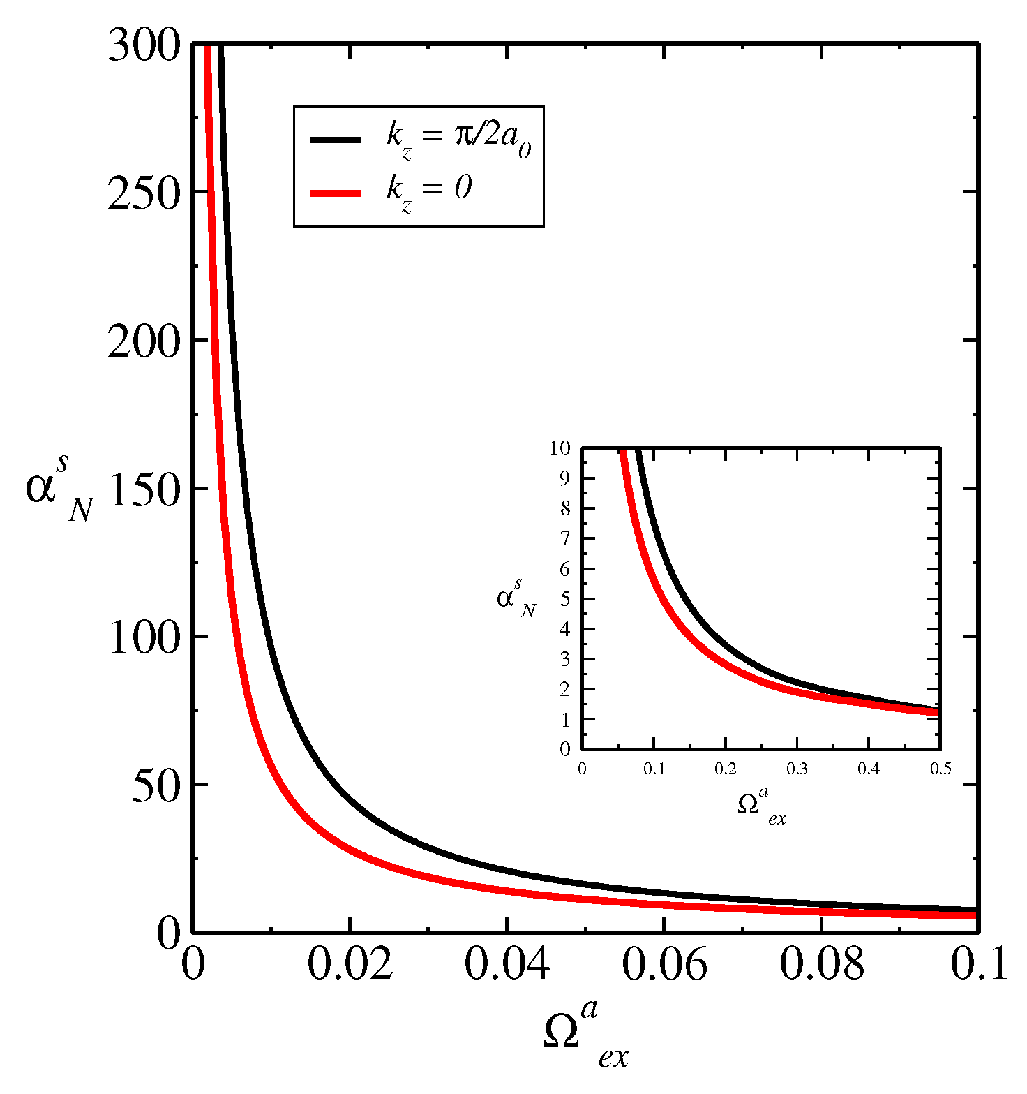
In Figure 4, we get the spin Nernst coefficient as a function of T for and , which corresponds to the Brillouin zone edge in the z direction. We have . We get that the very small variation of the curves of the spin Nernst coefficient as a function of T for different values and displayed in Figure 4, in the gap closing loop and where the system suffers a topological phase transition, generating a similar influence on the behavior of the curves of the entanglement negativity vs. T. In general, the spin Nernst effect introduces a non-equilibrium spin dynamics in the system, affecting the quantum correlations between spins, where depending on the strength of the spin-orbit coupling and the temperature gradient, the spin Nernst effect may influence the entanglement generation, propagation, or decay in the ferrimagnetic material. Thus, the interplay of spin Nernst effect, anisotropy, and quantum correlations may give rise to novel phenomena such as spin Hall effect described by the spin Nernst coefficient. The very small variation in the behavior of with is showed in the inset of the Figure 4, indicating thus, a small effect of the different magnon bands induced by on . In Figure 5, we get as a function of for held fixed, , and . Since depends on and biquadratic term , , , we obtain a dependence of with and in the same way. We get a small variation in the curves for different as showed in the inset of the Figure. The small variation obtained in the negativity and spin Nernst coefficient is a consequence of the small variation of the spin wave spectra with different intensities of external field along to the easy axis indicated by .
4. Outlook
In brief, we analyzed the influence of dipole-dipole interaction on spin Nernst coefficient and quantum entanglement in a lattice model given by the layered ferrimagnet. The quantities reported well as the contribution to the Nernst coefficient of a given plane in k-space and entanglement negativity are experimentally relevant [1,36]. It’s worth noting that the specific details and predictions regarding quantum correlations and spin Nernst effect would depend on the specific model, Hamiltonian, and parameters used in the study. We got that the changes reported in the quantities analyzed are very small, where the contributions from the analyzed planes in k-space are relevant or dominant [21]. Moreover, we get that the small change in the curves of the spin Nernst coefficient as a function of T, for different values and for , where the system suffers a topological phase transition, generating the same influence in the behavior of the curves of the entanglement negativity, vs. T. In a general way, the interplay of spin Nernst effect, entanglement negativity, and magnetism is a complex topic that requires further investigation and research. It is plausible that the spin Nernst effect influences the entanglement properties of the layered ferrimagnet by affecting the spin dynamics and correlations within the system. However, the specific details and quantitative aspects of this influence must depend on the particular characteristics of the material as well as its lattice structure and magnetic interactions.
Layered ferrimagnet with single-ion anisotropy K, external field with dipole-dipole interaction: The model is given by the Hamiltonian
where the unit vector is in the direction of the easy axis, specified to z (x) for the in-plane (out-of-plane) magnetized geometry, and is the unit vector pointed in the direction of the line joining of nearest-neighbors spins, and is the distance between them. Moreover, is the vacuum permeability constant, g is the Landé factor and is the Bohr magneton. The representation of the lattice considered is given in Figure 1. is the single-ion anisotropy and are the ferrimagnetic intra-layer exchanges. The notation used ℓ and i in denote the layer and the site, respectively. Being and for the sublattice a (d). Moreover, , and indicate the exchange constants between nearest-neighbors. The unit vector is the direction of the easy axis, which is specified to x direction in-plane (out-of-plane).
HP transformation: We performed the Holstein-Primakoff (HP) transformation expanded up to first order, after performing a local rotation of the spin operators of the model above to the new operators , and [21], so that the mean-field direction of the spins points along to the local z axis:
where we obtain the magnon Hamiltonian in the form of creation and annihilation operators, and , respectively.
Semimetal phase in collinear configuration: Whether the magnetic field is applied along to the easy axis with intensity below of the spin flop transition, we have a perpendicularly magnetized geometry, . The ferrimagnetic state is in the collinear configuration with the spins aligning in the z direction, corresponding to . The addition of the dipole-dipole interaction opens an anti-crossing gap at the intersection regions of the plane within the Brillouin zone, while the bands display linear crossings at the Brillouin zone edge, reflecting in the role of dipole-dipole interaction as a source of magnon spin-orbit coupling [21,22] and nontrivial magnon band topology [23,24]. We consider the dipole-dipole interaction as a perturbation, considering its smaller magnitude compared to the other energy terms and projecting the magnon Hamiltonian into a reduced subspace with the basis consisting of the eigenstates of the Hamiltonian excluding the dipole-dipole interaction.
In the collinear configuration, we take the discrete Fourier transform of the bosons operators
and the Bogoliubov transformation to get the dispersion relation of magnons [21]
where
and , , , . Furthermore, we have . corresponding to external field component along to the easy axis. In addition, we have the form factors
where the lattice spacing constant.
References
- N. Laflorencie, Physics Reports 646, (2016) 1.
- S. A. Owerre, Phys. Rev. B 95, (2017) 014422.
- L. S. Lima, Physica E 128, (2021) 114580.
- H. Katsura, N. Nagaosa, and P. A. Lee, Phys. Rev. Lett. 104, (2010) 066403.
- L. Zhang, J. Ren, J.-S. Wang, and B. Li, Phys. Rev. B 87, (2013) 144101.
- A. Mook, J. Henk, and I. Mertig, Phys. Rev. B 89, (2014) 134409.
- R. Matsumoto, R. Shindou, and S. Murakami, Phys. Rev. B 89, (2014) 054420.
- S. A. Owerre, Phys. Rev. B 94, (2016) 094405.
- S. A. Owerre, J. Phys.: Condens. Matter 28, (2016) 386001.
- P. Laurell and G. A. Fiete, Phys. Rev. B 98, (2018) 094419.
- K.-S. Kim, K. H. Lee, S. B. Chung, and J.-G. Park, Phys. Rev. B 100, (2019) 064412.
- L. Chen, Chin. Phys. B 28, (2019) 078503.
- A. Mook, J. Henk, and I. Mertig, Phys. Rev. B 99, (2019) 014427.
- Z.-X. Li, Y. Cao, and P. Yan, Phys. Rep. 915, (2021) 1.
- Z. Cai, S. Bao, Z. L. Gu, Y. P. Gao, Z. Ma, Y. Shangguan, W. Si, Z. Y. Dong, W. Wang, Y. Wu, D. Lin, J. Wang, K. Ran, S. Li, D. Adroja, X. Xi, S. L. Yu, X. Wu, J. X. Li, and J. Wen, Phys. Rev. B 104, (2021) L020402.
- F. Zhu, L. Zhang, X. Wang, F. J. dos Santos, J. Song, T. Mueller, K. Schmalzl, W. F. Schmidt, A. Ivanov, and J. T. Park et al., Sci. Adv. 7, (2021) eabi7532.
- A. Mook, K. Plekhanov, J. Klinovaja, and D. Loss, Phys. Rev. X 11, (2021) 021061.
- Z. Zhang, W. Feng, Y. Yao, and B. Tang, Phys. Lett. A 414, (2021) 127630.
- P. A. McClarty, Annu. Rev. Condens. Matter Phys. 13, (2022) 171.
- L. S. Lima, Eur. Phys. J. D 75, (2021) 28; Leonardo S. Lima Eur. Phys. J. D 73, (2019) 6; L. S. Lima, Eur. Phys. J. Plus 136, (2021) 789; L. S. Lima, J. Low Temp. Phys. 205, (2021) 112.; L. S. Lima, Physica A 483, (2017) 239; L. S. Lima, Physica A 492, (2018) 1853; L. S. Lima, J. Low Temp. Phys. 198, (2020) 241; L. S. Lima, J. Low Temp. Phys. 201, (2020) 515; Leonardo S. Lima, Eur. Phys. J. D 73, (2019) 242; L. S. Lima, Solid State Commun. 309, (2020) 113836; L. S. Lima, Solid State Commun. 295, (2019) 1; L. S. Lima, Physica E Low Dimens. Syst. Nanostruct. 141, (2022) 115235; L. S. Lima, Physica E Low Dimens. Syst. Nanostruct. 148, 115659 (2023); L. S. Lima, Eur. Phys. J. Plus 137, (2022) 1; L. S. Lima, Entropy 24, 1629 (2022); L. S. Lima, Int. J. Theor. Phys. 62, 93 (2023); L. S. Lima, J. Magn. Magn. Mater 590, (2024) 171673.
- J. Liu, L. Wang, K. Shen, Phys. Rev. B 107, (2023) 174404.
- K. Shen, Phys. Rev. Lett. 124, 077201 (2020).
- R. Shindou, J. -I. Ohe, R. Matsumoto, S. Murakami, E. Saitoh, Phys. Rev. B 87, 174402 (2013).
- Z. Hu, L. Fu, L. Liu, Phys. Rev. Lett. 128, 217201 (2022).
- L. E. Ballentine, Am. J. Phys. 55, (1986) 785.
- D. P. DiVincenzo, Science 270, (1995) 255.
- D. C. Marinescu, G. M. Marinescu, Approaching quantum computing, Pearson Prentice Hall, New Jersey, USA (2004).
- M. A. Nielsen, I. L. Chuang, Quantum Computing and Quantum Information, Cambridge University Press, Cambridge, UK (2000).
- A. R. Its, B-Q Jin, V. E. Korepin, J. Phys. A: Math. Gen. 38, (2005) 2975.
- J. I. Latorre, E. Rico, G. Vidal, Quant. Inf. Comput. 4, (2004) 48.
- D. Bianchini, O. A. Castro-Alvaredo, B. Doyon, E. Levi, F. Ravanini, J. Phys. A: Math. Theor. 48 04FT01 (2014).
- G. Vidal, J. L. Latorre, E. I. Rico, A. Kitaev, Phys. Rev. Lett. 90, (2003) 227902.
- J. I. Latorre, A. Riera, J. Phys. A.:Math. Theor. 42, (2009) 404002.
- K. Zyczkowski, P. Horodecki, A. Sanpera, M. Lewenstein, Phys. Rev. A 58, (1998) 883.
- G. Vidal, R. F. Werner, Phys. Rev. A 65, (2002) 032314.
- M. B. Plenio, Phys. Rev. Lett. 95, (2005) 090503.
- C. Castelnovo, Phys. Rev. A 88, (2013) 042319.
- Y. A. Lee, G. Vidal, Phys. Rev. A 88, (2013) 042318.
- C. Lanczos: An Iteration Method for the Solution of the Eigenvalue Problem of Linear Differential and Integral Operators, J. Res. Nat. Bur. Stand. 49, (1950) 255.
- G. H. Golub and C.F. van Loan: Matrix Computations (Johns Hopkins Univ. Press, (1996).
- W. E. Arnoldi: The Principle of Minimized Iteration in the Solution of the Matrix Eigen problem, Quarterly of Applied Mathematics 9, 17 (1951).
- Vladimir A. Zyuzin, Alexey A. Kovalev, Phys. Rev. Lett. 117, (2016) 217203.
- R. Cheng, S. Okamoto, Di Xiao, Phys. Rev. Lett. 117, (2016) 217202.
- B. Ma, Gregory A. Fiete, Phys. Rev. B 104, (2021) 174410.
Figure 2.
as a function of T using Lanczos Algorithm and Exact Diagonalization. We consider two different finite size lattice, sites (above graphic) and sites (below graphic). For all cases, we get a very small value for for all values of T, with tending to diverge at limit.
Figure 2.
as a function of T using Lanczos Algorithm and Exact Diagonalization. We consider two different finite size lattice, sites (above graphic) and sites (below graphic). For all cases, we get a very small value for for all values of T, with tending to diverge at limit.
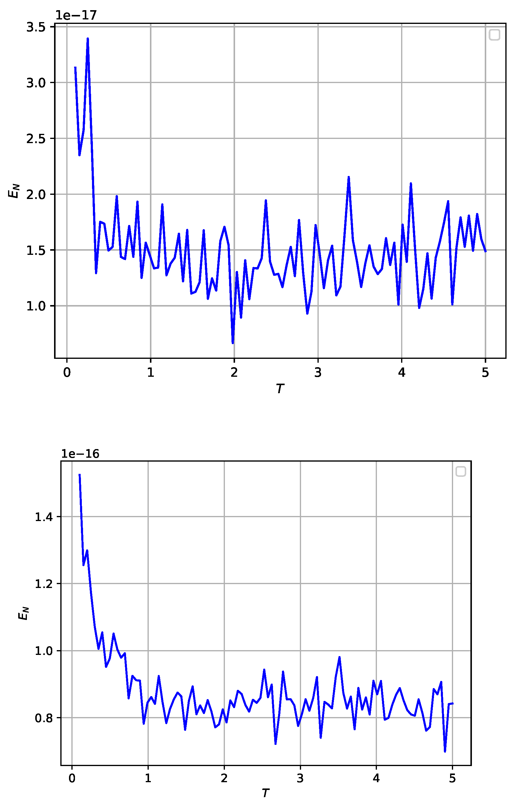
Figure 3.
as a function of T by SWT approach for , which corresponds to the Brillouin zone edge in z direction (above) and (below). We obtain . The value of corresponds to the value . We obtain a small difference of for the bands and .
Figure 3.
as a function of T by SWT approach for , which corresponds to the Brillouin zone edge in z direction (above) and (below). We obtain . The value of corresponds to the value . We obtain a small difference of for the bands and .
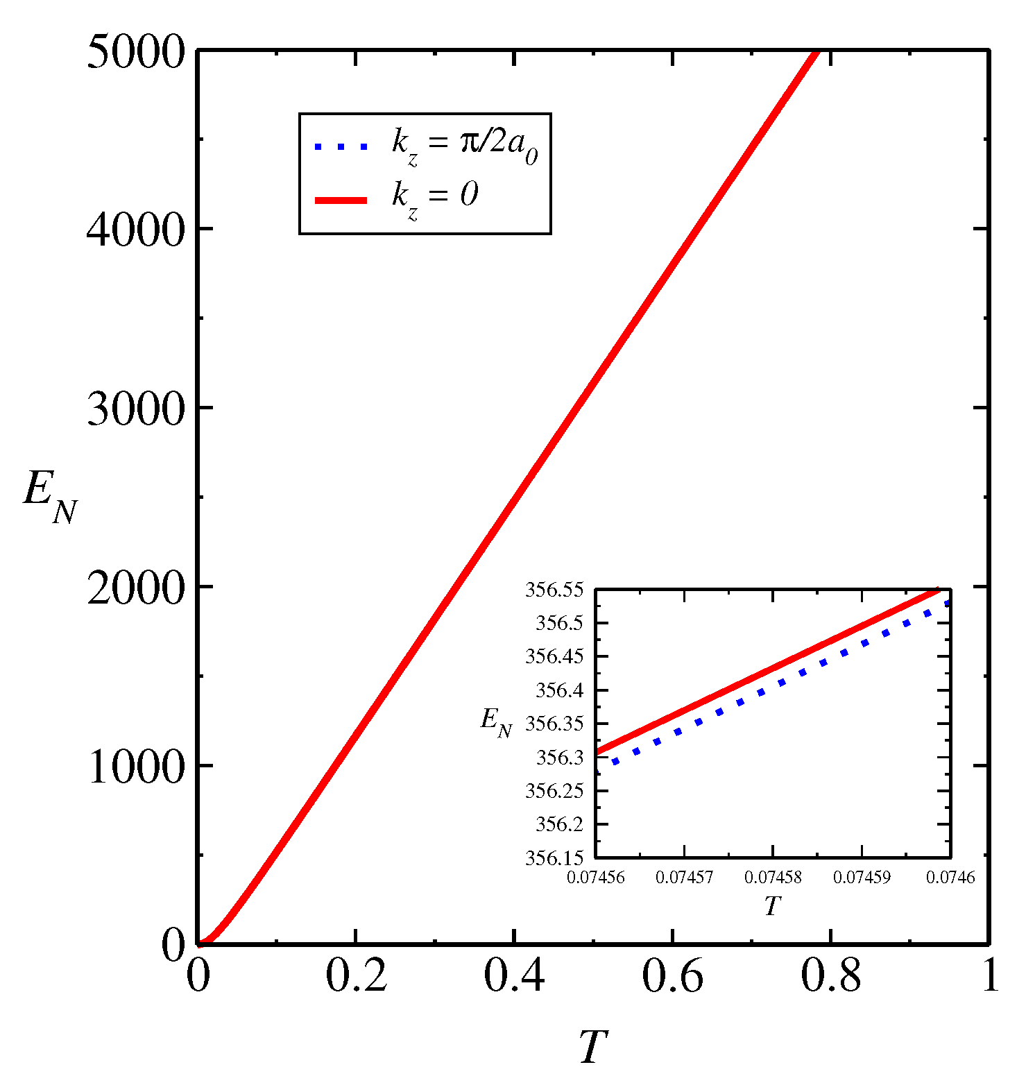
Figure 4.
as a function of T for , and . We have a dependence on anisotropy constant of given by .
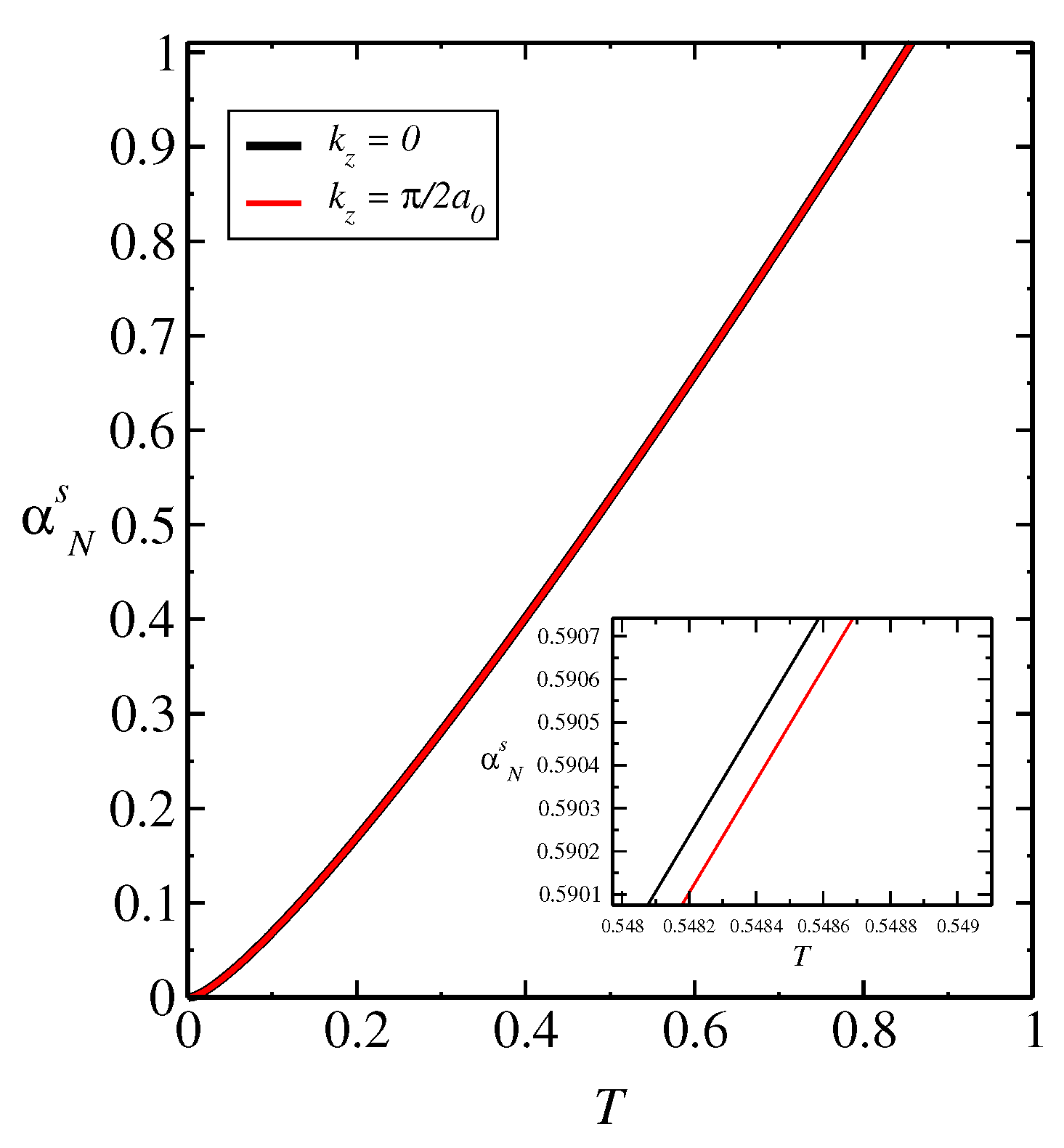
Figure 5.
as a function of for held fixed for , and . We have a dependence of on and anisotropy constant given by .
Figure 5.
as a function of for held fixed for , and . We have a dependence of on and anisotropy constant given by .
Disclaimer/Publisher’s Note: The statements, opinions and data contained in all publications are solely those of the individual author(s) and contributor(s) and not of MDPI and/or the editor(s). MDPI and/or the editor(s) disclaim responsibility for any injury to people or property resulting from any ideas, methods, instructions or products referred to in the content. |
© 2024 by the authors. Licensee MDPI, Basel, Switzerland. This article is an open access article distributed under the terms and conditions of the Creative Commons Attribution (CC BY) license (http://creativecommons.org/licenses/by/4.0/).
Copyright: This open access article is published under a Creative Commons CC BY 4.0 license, which permit the free download, distribution, and reuse, provided that the author and preprint are cited in any reuse.


