The More Complex, The Deeper: SchNet+ as an Improved Neural Network for Complexity in Quantum Materials

1. Introduction

The complex form of equations and their unsolvability in quantum world is a permanent trouble for quantum physicists, especially from the perspective of quantum-material-rooted researchers [1]. For exemplification, the multi-electron systems are a kind of typical system, which can not be solved in a mathematically precise manner, which is to say, the basic ones like Schrödinger equation or the Dirac equation fail in depicting such a complicated system with innumerable interactions. As a consequence, quantum physicists turn their attention to numerical methods instead of sticking to analytical solutions. Fortunately, deep learning provide a option to untangle the intricate scenario respectively effectively. Previous studies have adopted a diversity of methods to get a more precise prediction: The original trying was made by PINN [2], which use a loss function added the deviation of the differential equation in order to constrain the model to obey the quantum laws; Some progress was made by [3], which use a deep convolutional neural network (CNN) [4] to narrate the interaction between the electrons; It is remarkable that the SchNet [5] groundbreakingly ultilize graph neural network (GNN) [6], a good-at-handling-interaction network, to tackle with the complexity. Compared with the tradictional multi-layer-perceptron-only model, the facaulty of narrating the interactions is significantly enhanced, which renders the SchNet a more powerful tool. Nevertheless, some problems still exist:

• The SchNet concentrates on depicting the interactions but neglects the strength of perceptron more complicated phenomenon.
• The physical constraints are specially designed in SchNet, but they are not sufficient to describe the complex situation.
• The original activation function ReLU can be provocative of the gradient vanishing problem, which is a major problem in deep learning.

In this work, we proposed a new neural network SchNet+ based on SchNet, which aims to solve the problems listed above.

2. Related Work

Previous work has used many techniques aiming to improve the capability of the model and restrict the model not to intervein the physical laws. GNN, RBF and ResNet are some of the methods in vogue.

2.1. Graph Neural Network (GNN)

Graph is a high-level-of-freedom data structure that can be used to present the relationship between nodes, edges and the whole graph. GNN, which based on graph structure, is undoubtedly a powerful tool to solve the complex problem.

Figure 1. The Graph Neural Network.

Figure 1. The Graph Neural Network.

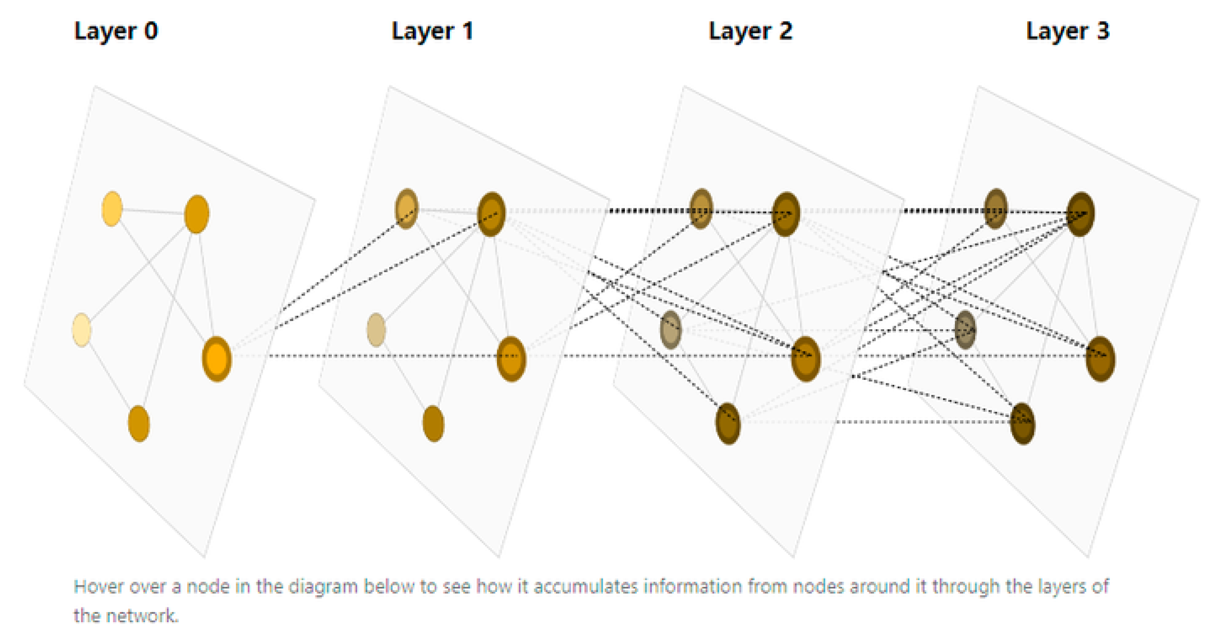
Concerning the complexity of the systems in quantum matreials, GNN plays an important role in coping with the interaction between the particles.

2.2. Radius Basis Function (RBF)

RBF [7] is extremly useful in describing the positions of particles by mapping it to another basis function space (usually Gaussian) to have the model better understand and deal with the position vectors. By choosing appropriate hyperparameters (e.g. the number of basis functions, the width of the basis functions, etc.), the efficiency of the model can be well optimized.

If Gaussian basis functions are used, the steps below can be approached:

1.

Uniformly select k points as the centers of the basis functions, where the number of centers k, the positions of the centers $\mu$, the distances between adjacent centers $\sigma$ are hyperparameters;

2.

Calculate the Euclidean distance from each nodes to each basis function centers:

$$dis{t}_{i,k}=po{s}_i-{\mu }_k$$

3.

Calculate the Gaussian function respectively:

$$g_{i,k}={\displaystyle \frac{e^{dis{t}_{i,k}^2}}{2{\sigma }^2}}$$

4.

Then $(g_{i,1},g_{i,2},\dots ,g_{i,k})$ is the cordinate of the node in the basis function space.

2.3. Residual Neural Network (ResNet)

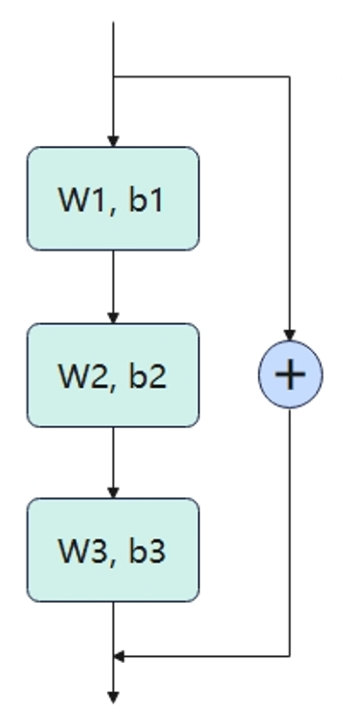
The deep learning was confronting a serious problem: the performance stops to improve or even degrades after a certain depth of the network. In 2015, He’s team proposed ResNet to resolve the demanding problem in a quite simple way, which is to add a residual connection to the network.

Linear layers are supposed to make predictions $\widehat{y}$ from input data x directly in the past, but without any layer-layer connection, the parameters may be against each other, causing the deterioration of the performance. Contrarily, linear layers with residual connections are supposed to predict $\widehat{y}-x$ from x, which allows linear layers to learn indentical mappings, guaranteeing the performance not to decline at least.

Figure 2. The Residual Neural Network.

Figure 2. The Residual Neural Network.

3. Appraoch

3.1. SchNet: The Baseline Model

SchNet is chosen as the baseline model on account of its structural potential in describing the complex interaction. By using GNN and RBF, the realationship between several particles can be beautifully described. However, when the situation is getting intricater, the performance of SchNet is not enough to satisfy the requirement. It can be noted that the depth of SchNet is only 2 when updating vertices, 1 when updating edges and globality, which absolutely limits the capability of the model. Additionally, SchNet ultilizes Gradient-Domain Machine Learning [8] as physical constraints without adding any differential-equation-based constraints, which could be a drawback as well.

3.2. SchNet+: The Improved Version

Figure 3. The SchNet+ Structure.

Figure 3. The SchNet+ Structure.

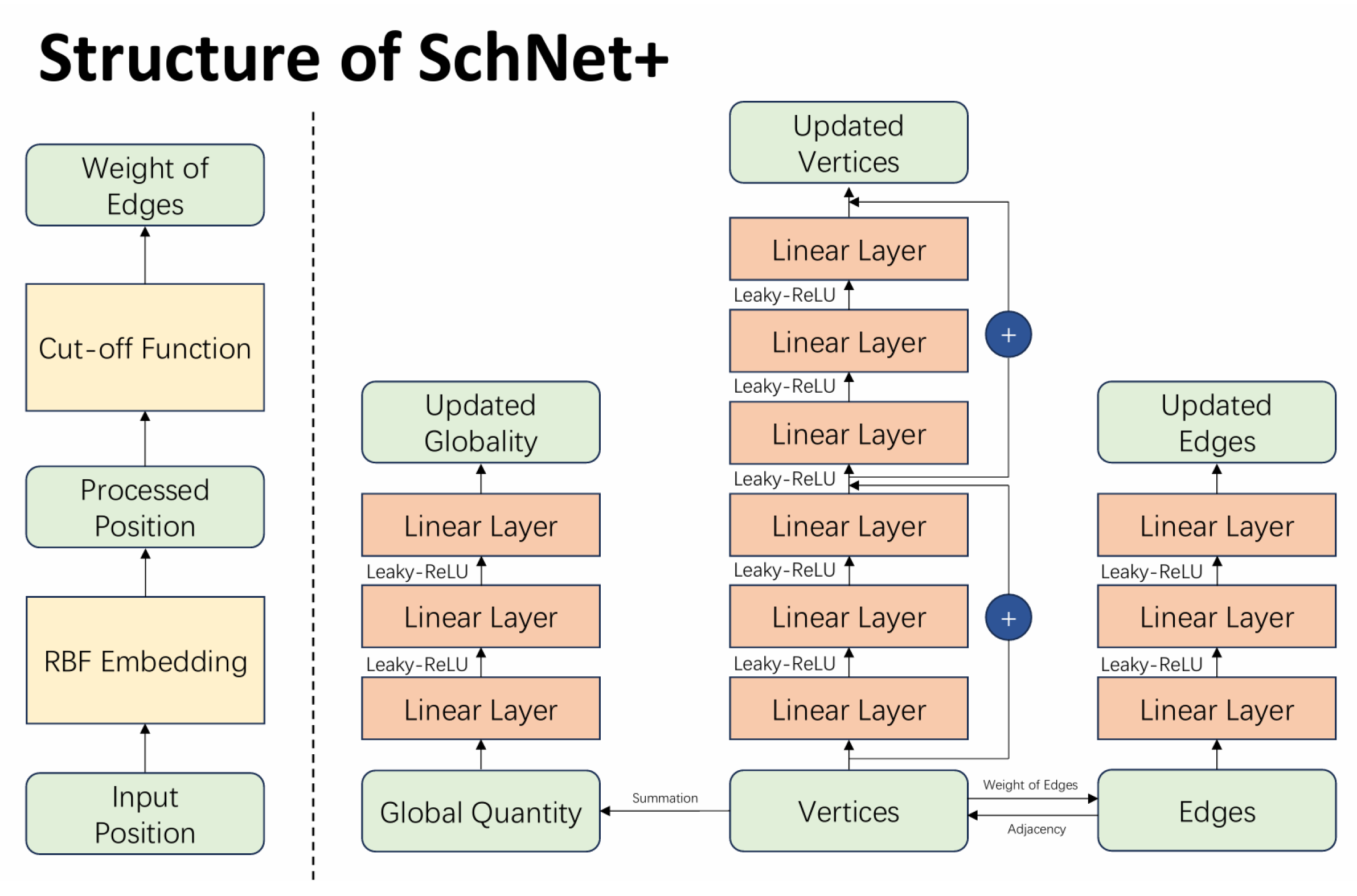
3.2.1. Deeper MLP

The depth of MLP in neural network is one of the key factors that determines the capability of the perceptron. In one hand, the deeper MLP is, the more parameters the model has, the more powerful the model is; in the other hand, the deeper MLP is, the more likely the model will overfit, and more time and memory will be needed to train the model. Therefore, selecting a proper depth of MLP is vital for SchNet+. Due to the limitation of the accessible computational resources, the optimal depth of MLP is not precisely determined, but an approximate range from 6 to 10 when updating the vertices and from 1 to 3 when updating the edges and globality is suggested, according to some experienment on some small scale datasets.

3.2.2. Applied ResNet

Owing to the depth of MLP comes up to at least 6 when updating the vertices of SchNet+, the risk of overfitting and the violation of physical laws is higher. Thus ResNet is naturally applied to SchNet+. That each 3 linear layers are combined into a residual block in SchNet+ is properly adopted.

3.2.3. More Potential Activation Functions

Considering the depth of MLP in SchNet+, an inproper activation function would be deadly for the neurons. LeakyReLU [9], as an improvement of ReLU, is utilized to substitude former ReLU as the activation function in case of gradient vanishing. The result of experienment demonstrates that SchNet+ with LeakyReLU performs better in terms of loss descent process.

3.2.4. New Physical Constraints

In SchNet+, the energy conservation constraint is retained for its excellent property. Furthermore, the rotational invariance and some symmetry are added to the loss function as basic physical laws; some contingent equantional deviations are also taken into consideration for their possibily impact on the model’s performance.

As a matter of fact, 3.2.2, 3.2.3 and 3.2.4 are natural adaptations for the deeper MLP, which is mentioned in 3.2.1. The Logic is as follows: SchNet+ is designed to be a complicated-situation-processor, so the deeper MLP is the core, and some other adaptations like ResNet, Leaky-ReLU and new physical constraints are used to resolve the possible problems of more complexity in the model.

4. Experienment

A sample experienment is conducted on a small scale dataset, which is a simple situation of predicting the energy of a single water molecule. The dataset is obviously SchNet-friendly, but the performance of SchNet+ still catches up with and even outperforms SchNet.

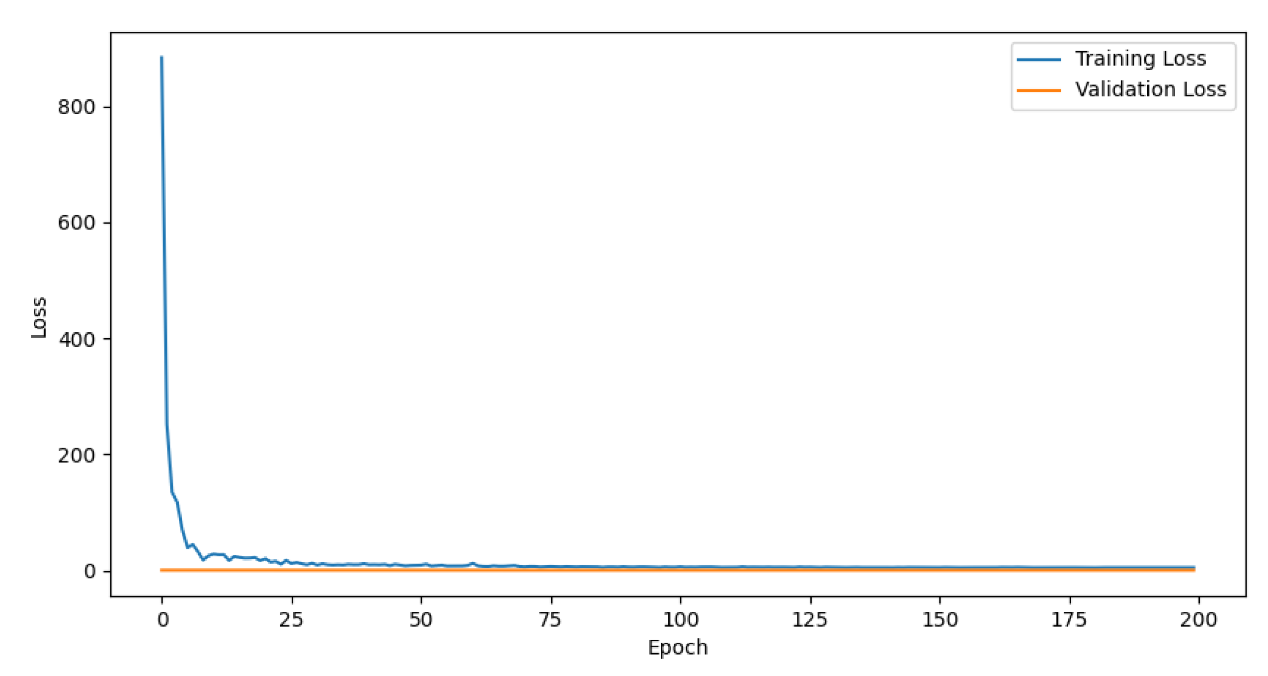
The loss descent process is shown in the figure below:

Figure 4. The Loss Descent Process of SchNet.

Figure 4. The Loss Descent Process of SchNet.

Figure 5. The Loss Descent Process of SchNet+.

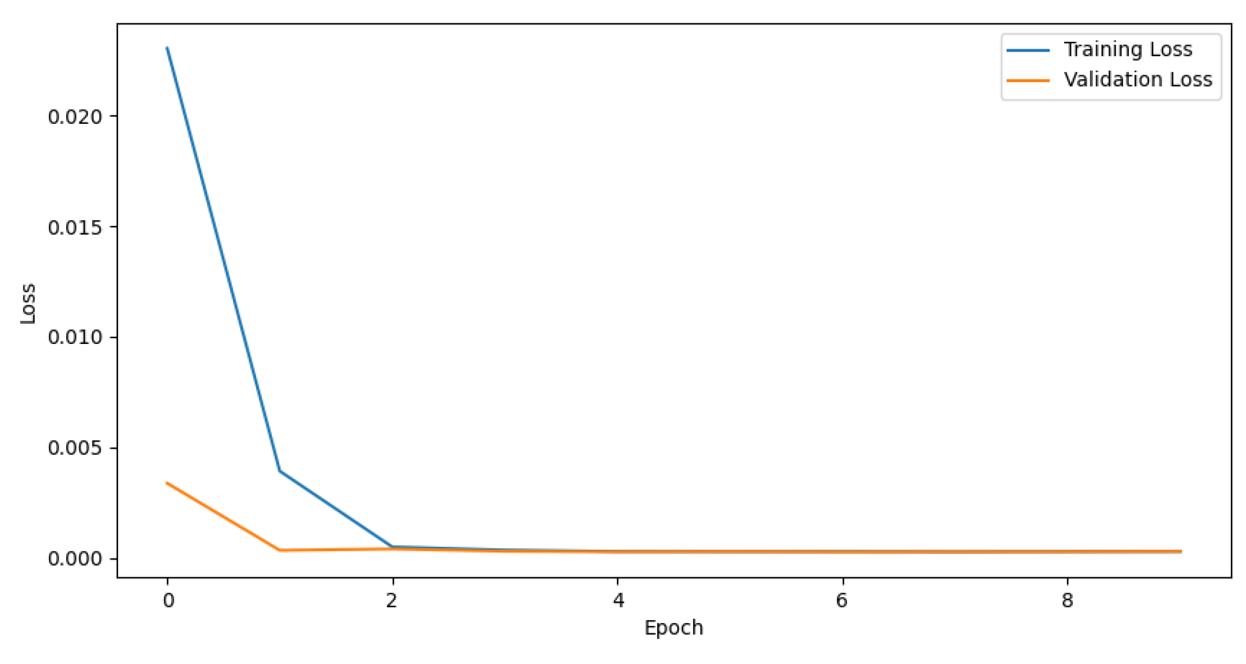
Figure 5. The Loss Descent Process of SchNet+.

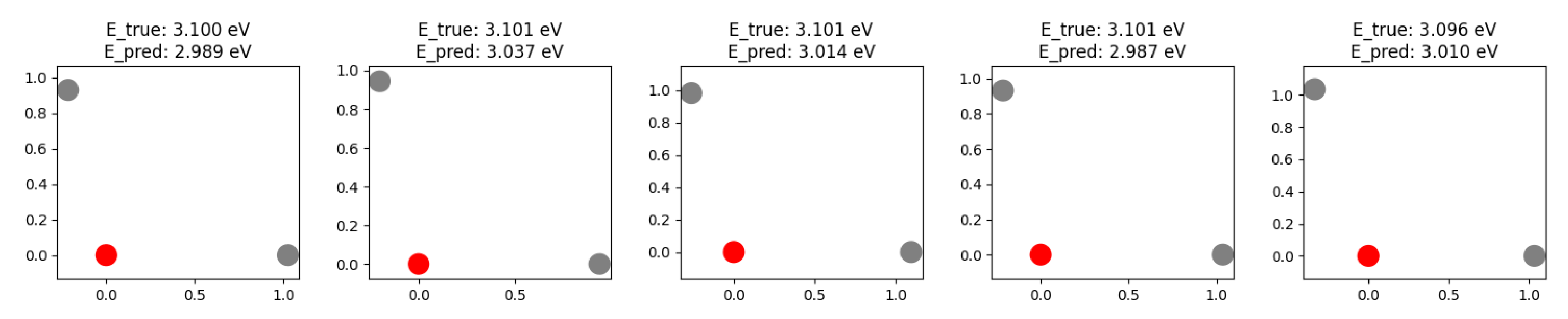
The random sample of prediction vs real value is shown in the figure below:

Figure 6. The Prediction vs Real Value of SchNet.

Figure 6. The Prediction vs Real Value of SchNet.

Figure 7. The Prediction vs Real Value of SchNet+.

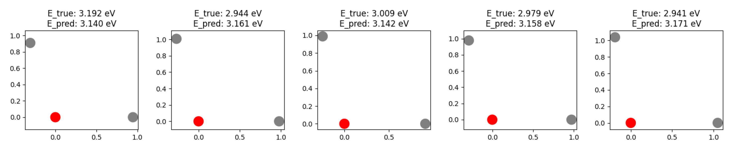
Figure 7. The Prediction vs Real Value of SchNet+.

The error distribution is shown in the figure below:

Figure 8. The Error Distribution of SchNet.

Figure 8. The Error Distribution of SchNet.

Figure 9. The Error Distribution of SchNet+.

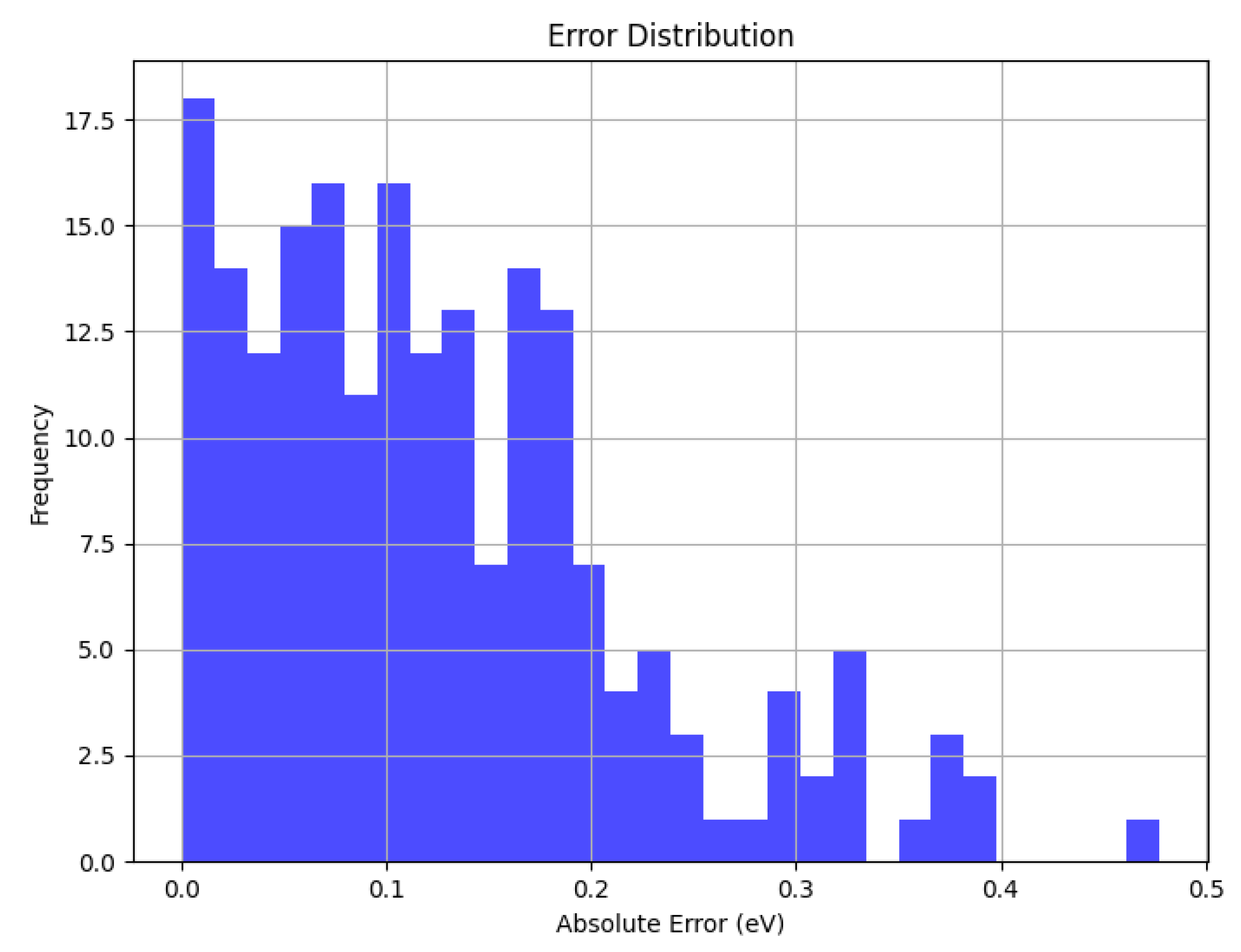
Figure 9. The Error Distribution of SchNet+.

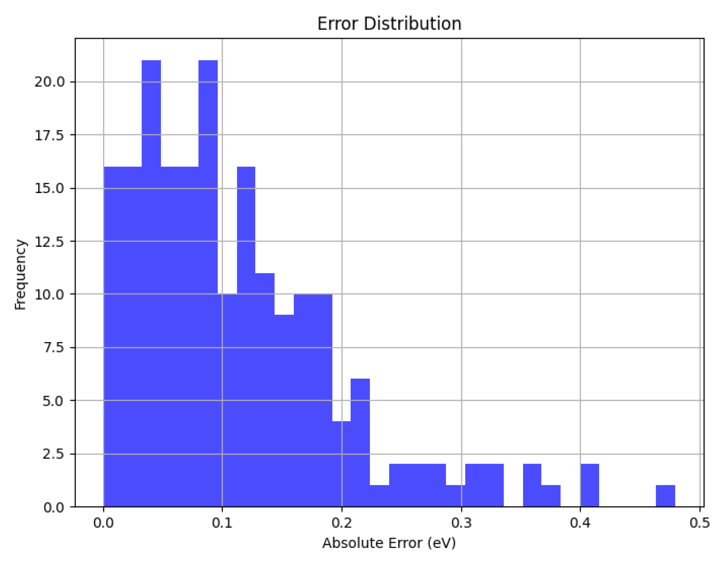
It can be noted that the performance of SchNet+ is not worse than that of SchNet in the dataset which is more suitable for SchNet. Thus when it comes to the more complex situations, SchNet+ is anticipated to perform far beyond SchNet, i.e. SchNet+ is a more favourable model than SchNet, especially in the complex situations. However, what must be mentioned is that the training time of SchNet+ is much longer than the original version on account of the increased complexity of the model.

5. Discussion

5.1. Limitations

It is universally acknowledged that deeper MLP leads to more powerful perceptrons, but a much longer training time is required. It may be expensive to train a SchNet+ if time and hardware is strictly limited or a tiny dataset is provided. In that case, a more simple but effective method is to turn back to SchNet, which is also a good choice for simple cases.

Table 1. The Comparison between SchNet and SchNet+.

	Pros	Cons
SchNet	Low training cost, Good for simple cases	Bad for complex cases
SchNet+	Good for complex cases	High training cost

Table 1. The Comparison between SchNet and SchNet+.

	Pros	Cons
SchNet	Low training cost, Good for simple cases	Bad for complex cases
SchNet+	Good for complex cases	High training cost

5.2. Future Work

Some possible future work is listed below:

• Attention Mechanism [10] is also a powerful tool to handle interactions, which possibly outperforms GNN in SchNet+. If multi-head attention is adopted, the model possibly performs better.
• The hyperparameters in procvided SchNet+ sample may be not optimal. By using meshgrid search or other hyperparameter optimization methods, which may cost more training time and better GPU, the property of SchNet+ is expected to be improved.
• The physical constraints in both SchNet and SchNet+ are added to the loss function instead of embedding in the model, which may provoke the deviation from the real situation. If some of the constraints are internalized, the model would have a stronger ability to fitting the reality.

6. Conclusion

In this work, a new neural network SchNet+ is proposed to dealing with intricater scenarios in quantum materials. The better performance of SchNet+ is guarateed by deeper MLP, ResNet, LeakyReLU and new physical constraints, which are of much help proved by the sample experienment. SchNet+ furnishes the opportunity to make the prediction in complicated cases much easier and more precise. With the future work raised in the Discussion, SchNet+ is expected to be a more powerful tool in quantum materials.

References

- Anderson, P.W. More Is Different. Science 1972, 177, 393–396, http://arxiv.org/abs/https://www.science.org/doi/pdf/10.1126/science.177.4047.393. [CrossRef]
- Raissi, M.; Perdikaris, P.; Karniadakis, G. Physics-informed neural networks: A deep learning framework for solving forward and inverse problems involving nonlinear partial differential equations. Journal of Computational Physics 2019, 378, 686–707. [CrossRef]
- Mills, K.; Spanner, M.; Tamblyn, I. Deep learning and the Schrödinger equation. Phys. Rev. A 2017, 96, 042113. [CrossRef]
- Kim, Y. Convolutional Neural Networks for Sentence Classification, 2014, [arXiv:cs.CL/1408.5882].
- Schütt, K.T.; Kindermans, P.J.; Sauceda, H.E.; Chmiela, S.; Tkatchenko, A.; Müller, K.R. SchNet: A continuous-filter convolutional neural network for modeling quantum interactions, 2017, [arXiv:stat.ML/1706.08566].
- Zhou, J.; Cui, G.; Hu, S.; Zhang, Z.; Yang, C.; Liu, Z.; Wang, L.; Li, C.; Sun, M. Graph neural networks: A review of methods and applications. AI Open 2020, 1, 57–81. [CrossRef]
- A Review of Radial Basis Function (RBF) Neural Networks. In Radial Basis Function Neural Networks with Sequential Learning; pp. 1–19, [https://worldscientific.com/doi/pdf/10.1142/9789812812506_0001]. [CrossRef]
- Chmiela, S.; Tkatchenko, A.; Sauceda, H.E.; Poltavsky, I.; Schütt, K.T.; Müller, K.R. Machine learning of accurate energy-conserving molecular force fields. Science Advances 2017, 3, e1603015, [https://www.science.org/doi/pdf/10.1126/sciadv.1603015]. [CrossRef]
- Xu, B.; Wang, N.; Chen, T.; Li, M. Empirical Evaluation of Rectified Activations in Convolutional Network, 2015, [arXiv:cs.LG/1505.00853].
- Vaswani, A.; Shazeer, N.; Parmar, N.; Uszkoreit, J.; Jones, L.; Gomez, A.N.; Kaiser, L.; Polosukhin, I. Attention Is All You Need, 2023, [arXiv:cs.CL/1706.03762].
Disclaimer/Publisher’s Note: The statements, opinions and data contained in all publications are solely those of the individual author(s) and contributor(s) and not of MDPI and/or the editor(s). MDPI and/or the editor(s) disclaim responsibility for any injury to people or property resulting from any ideas, methods, instructions or products referred to in the content. |
© 2025 by the authors. Licensee MDPI, Basel, Switzerland. This article is an open access article distributed under the terms and conditions of the Creative Commons Attribution (CC BY) license (http://creativecommons.org/licenses/by/4.0/).
Copyright: This open access article is published under a Creative Commons CC BY 4.0 license, which permit the free download, distribution, and reuse, provided that the author and preprint are cited in any reuse.