
Submitted:
26 October 2024
Posted:
28 October 2024
You are already at the latest version
Abstract
Today, the facility location planning issue mainly belongs to the long-term operational and strategic level of large public and private organizations, and the significant costs associated with facility location, construction, and operation have turned location research into long-term decision-making. Presenting a hub location model for the green supply chain can address the current status of facilities and significantly improve demand coverage at an acceptable cost. Therefore, in this study, a network of facilities for hub location in the service site domain, considering existing and potential facilities under probable scenarios, has been proposed. After presenting the mathematical model, validation was performed on a small scale, followed by sensitivity analysis of the main parameters of the model. Furthermore, a metaheuristic algorithm was employed to analyze the NP-Hardness of the model. Additionally, to demonstrate the efficiency of the model, two metaheuristic algorithms, NSGAII and MOPSO, were developed. Based on the conducted analysis, it can be observed that the computational time increases exponentially with the size of sample problems, indicating the NP-Hardness of the problem. However, the NSGAII algorithm performs better in terms of computational time for medium-sized problems compared to the MOPSO algorithm.
Keywords:
Facility Location
; maximum coverage
; telecommunication
; Hub Location
; NSGAII
; MOPSO
1. Introduction
The issue of facility location planning, especially in the domain of public health facilities, is significant [1]. The term “facility location” refers to the process of determining the optimal locations for facilities where services are provided to a certain population. Facility location involves considerations such as accessibility, service coverage, cost-effectiveness, and the socio-economic impact of the facility location on the surrounding community. In the context of healthcare facility location, it entails determining the optimal locations for the establishment of medical facilities to provide timely and effective healthcare services to the population [2]. Several studies and research have been conducted in the field of hub location so far [3,4,5,6]. including both emergency and non-emergency facilities. However, a crucial aspect that has received less attention so far is the comprehensive evaluation of facility locations’ efficiency [7,8]. This entails assessing whether the decisions made over time regarding the location of facilities, considering various needs and constraints, are collectively optimal. Therefore, it is essential to comprehensively examine whether the chosen hub locations are optimal across different time periods and in relation to each other [9]. Therefore, the topic of optimal hub location is raised in a multidimensional manner, where the aim is to comprehensively and systematically examine the optimality of hub locations across the entire target region, and if necessary, to carry out hub location [10]. This hub location may involve establishing new hubs, removing existing hubs, increasing or decreasing the capacity of a hub. If the location is not considered for the target area, we will face a number of local optimal solutions, each obtained at a specific time, which not only may not provide us with a globally optimal solution but also does not consider the changes in demand over time in the covered areas after the location is determined [11]. One of the challenges in the hub location problem is considering the hubs at different points equally and with similar services and capacities. This is because the characteristics of the selected locations, constraints, and the type and amount of needs in each area are not necessarily similar to each other, and these differences make uniform facilities not have sufficient efficiency [12]. From these differences, we can, for example, mention the following: In an area with a high population density, there is a need for facilities with high capacity, or in an area where there are suitable and extensive access routes, the coverage radius of a hub can be greater than other hubs or the types of needs may vary in different areas and require hubs with different services [13]. Despite these conditions, to reach an optimal solution, facilities with different characteristics and capacities should be considered. This is known in location literature as hub location, and considering this feature can lead to a more suitable solution for the problem [14]. In the field of hub location in various domains, including healthcare, uncertainty is one of the influential factors. For various facilities, many parameters such as the amount, type, and timing of demand creation are uncertain, and considering this uncertainty in the parameters can increase the practicality of the problem [15]. One of the assumptions that has been prevalent in location problems in the past is the assumption of facilities operating under different conditions [16]. However, this assumption is not valid in the real world, and facilities may be disrupted due to various reasons such as pollution and environmental issues, causing their activities to be halted [17]. The reasons for disruptions can be natural, such as disruptions due to the failure of wastewater and air catalysts, or human-induced, such as disruptions in the performance of air, water, and soil settlement due to operational errors [18]. Therefore, considering the probability of disruptions in pollutant production and providing a model that can continue its work under environmental disruption conditions is of paramount importance and high applicability [14]. In this article, we also attempt to provide a model that addresses hub location in a green state by considering environmental disruptions. Another aspect to consider in hub location is the limitations present in facility capacities and communication routes. Each facility has a limited capacity based on various factors, and it cannot provide services beyond this capacity. Therefore, considering limited capacities for facilities is necessary, and if these constraints are not considered, we deviate from real conditions, and the model will not be practical. On the other hand, many hub location problems have multiple objectives [19,20,21].
The objectives commonly considered in hub location problems are summarized below. Cost is one of the most common objectives in hub location problems [5]. Costs come in various types, divided into variable and fixed costs. Variable costs include installation expenses, while fixed costs include relocation expenses [15]. Typically, in hub location problems, a unified objective comprising all types of costs is considered. Another objective is coverage, which is used in maximal coverage problems. In this case, an objective is added to the model to maximize demand coverage. Other objectives exist in hub location problems, but we will not delve into them here. In this study, we aim to establish a balance between objectives such as maximizing demand coverage, minimizing costs, and maximizing greenness in the hub location.
This article presents a multi-objective mathematical programming model in which the objectives of cost, demand coverage, and greenness of location are considered, aiming to address hub location under a comprehensive perspective to examine the optimality of the current facility locations and, if necessary, relocate existing facilities or locate new facilities. In order to find an effective and efficient solution, factors of uncertainty are also addressed. Given the nature of the problem under study and researchers’ opinions, the hub location model is NP-HARD. To validate the mathematical model, initially, the Pareto front of optimal solutions will be evaluated using an epsilon-constraint approach, and ultimately, to validate the model on larger scales, metaheuristic algorithms will be utilized. This article consists of five sections. The first section discusses the problem under study. The second section reviews the research literature, and the third section presents the mathematical model. The fourth section analyzes the mathematical model, and finally, conclusions and future research recommendations are provided.
2. Problem Description
In this proposed model, it is assumed that there are several facilities at different levels in the region under study. Given that the existing facilities have been established over a long period spanning several years and considering that changes have occurred in the level and concentration of demand for services by customers during these years, it is necessary to comprehensively evaluate all existing hubs. In this section, initially, the existing hubs in the region for transporting network equipment are classified into three levels, and then the demand coverage by these facilities is examined. If there is a justifiable change in the capacity or location of the facilities in terms of cost, these changes are made in the location and capacity of the existing facilities. Finally, a new structure of hub location is proposed in which the location and capacity of some hubs have changed, but in return, the demand coverage for telecom services has increased. Improving demand coverage is not only done by examining the capacity level of existing hubs and adjusting their locations. In this article, three levels of capacity are also considered for the hubs, and if necessary, a hub is upgraded to a higher capacity level, or a new hub is located. To improve the quality of demand coverage for customers, the coverage radius is also considered for each hub. The coverage radius helps allocate demand to hubs in such a way that the distance from the demand point to the hub is optimized and acceptable. In this article, the coverage radius is considered as a variable. Since the level of demand coverage is directly related to the distance from the demand point to the hub and the variable coverage cost, efforts are made to minimize the coverage radius of each hub. In improving the current situation, only changes to existing hubs are not addressed, and if there is a need for locating a new hub, a new hub is established. In this problem, we aim to examine the efficiency of existing hubs in terms of coverage capacity and locate new hubs with the goal of reaching a higher level of demand coverage, reducing costs, and maximizing the level of greenness in hub locations. To this end, in our analysis, we consider the economic feasibility of the following actions: establishing new hubs, removing previous or existing hubs, and increasing or decreasing the capacity of hubs.
2.1. Assumptions of the Problem
The study area is divided into several regions. Regions are subsets of a larger area called zones, which are covered by hubs.
In this study, three levels of hubs are considered: level w hubs, which have the lowest capacity level and provide primary services. Level c hubs provide complementary services. Finally, level h hubs provide the most advanced services and also provide level c hub services.
Each demand point must be covered by one level w hub, one level c hub, and one level h hub. However, Level H hubs can also provide Level C hub services. Therefore, if a demand point is covered by a level h hub, there is no need for it to be covered by a level c hub.
In each region, there must be at least one level w hub.
In a region, it is not possible to have both level c and level h hubs simultaneously.
In a zone, there cannot be more than one level h hub.
Demand is considered to be point-wise.
In Figure 1, different scenarios of demand coverage based on the assumptions are depicted. In the first scenario, the demand point is allocated to all three available levels of hubs. In this case, the demand for each level is assigned to hubs of the same level. In the second scenario, the demand point is allocated to two hubs at levels w and h. In this case, as described in the assumptions, the demand for level c is covered by the level h hub because level h hubs can provide services for level c hubs as well.
2.2. Mathematical Model
In this proposed model, it is assumed that there are several hubs at different levels in the studied area, and the level of demand coverage by these hubs needs to be examined. If there are changes in the capacity or location of the hubs that are economically justified, these changes in the location and capacity of the existing hubs are made. Ultimately, a new structure of hubs is presented, where the location and capacity of some hubs have changed, but the demand coverage has increased. In this section, the mathematical model of the research is presented.
We seek to examine the efficiency of existing hubs with the goal of achieving a higher level of demand coverage. To this end, in our analysis, we consider the economic viability of the following actions: establishment of hubs, removal of hubs, increase, and decrease in facility capacity.
Sets, indices, parameters, and decision variables in this section are introduced.
Sets and Indices
| Set of Network Points | |
| Set of Regions in the Model | |
| Set of Zones in the Model | |
| Set of Uncertainty Scenarios | |
| Set of nodes available in region r | |
| Index related to the level of hub capacity. | |
| Index related to the region. | |
| Index related to the region. | |
| Index related to each scenario. |
Parameters.
| The fixed cost of establishing a hub at level l at point j with capacity level t. | |
| The level of greenness of the hub at level l at point j with capacity level t. | |
| The capacity level associated with level t. | |
| 1 if a hub at level l exists at point j with capacity level t; 0 otherwise. | |
| The number of hubs at level l that must exist at the end. | |
| The distance between two points i and j. | |
| Maximum acceptable coverage radius. | |
| Acceptable deviation level from the optimal amount for each scenario in the original model. |
Decision variables
| Optimal demand coverage level in each scenario | |
| Optimal cost in each scenario | |
| 1 if demand at point i is covered; 0 otherwise | |
| 1 if level-i hub at point j with capacity level t does not exist previously; 0 otherwise | |
| The coverage radius of the hub existing at point j | |
| 1 if demand point i is allocated to hub j at level l in scenario s; 0 otherwise. | |
| 1 if hub of level l exists at point j with capacity level t; 0 otherwise. |
Objective Functions and Constraints
Given the sets, indices, parameters, and decision variables presented in the previous section, the objective functions and constraints of the proposed model are provided as follows.
s.t.
Objective Function (1) represents the amount of demand covered. Objective Function (2) represents the cost incurred due to changes in the structure of hubs, where a binary variable takes a value of one if a new hub is located or if there is a change in the capacity of a hub or its relocation, and the cost of this change is calculated. In the second part of the equation, the cost of the coverage radius of each hub is calculated as a function of the radius. Objective Function (3) maximizes the level of greenness in the hub location. Each demand point is covered only if it is allocated to at least one hub at level w and one hub at level h in its own region; this condition is considered in equation (4). According to the model assumptions, a hub at level h can make a demand point unnecessary to be allocated to a hub at level c; therefore, in equation (), this assumption is applied that allocating a demand point to a hub at level h in one region does not necessarily require assigning that point to a hub at level c.
Equation (5) expresses the requirement to establish at least one level-w hub in each region. The assumption of the prohibition of simultaneously establishing two hubs at levels h and c in one region is considered in equation (7). Equation (8) limits the establishment of more than one level-h hub in one region. Equation (9) restricts the establishment of more than one hub at a single point. Equation (10) represents constraints on the availability and capacity of hubs, preventing the allocation of more than the optimal capacity level to hubs and also preventing demand allocation to hubs in scenarios where the hub is unavailable. Equations (11) and (12) determine the coverage radius of each hub. Equation (13) indicates the permissible number of network changes at each level. Equation (14) identifies whether a hub has undergone changes during hub location or remained unchanged. Equations (15) and (16) ensure that the objective function value does not deviate by more than the allowable percentage from the optimal value in each scenario.
2.3. Solving the Proposed Model (Modified Epsilon-Constrained Approach)
In multi-objective problems, there is generally no single optimal solution that simultaneously optimizes all objective functions. Therefore, the concept of optimality is replaced with Pareto optimality or efficiency. Pareto optimal solutions (efficient, non-dominated) are solutions that cannot improve one objective function without worsening the performance of at least one other objective function (Fonseca, 2016). The Pareto set is a set of Pareto optimal solutions.
According to Huang and Masoud (2012), there are three main approaches for solving multi-objective optimization problems based on decision maker preference elicitation: a priori methods, a posteriori or generative methods, and interactive methods. In a priori methods, the decision maker provides their preferences before the process begins. This method has the drawback of reducing preferences determined by the decision maker. A posteriori methods involve optimizing all objective functions simultaneously. In this approach, the Pareto set is first generated. Then, at the end of the search process, the decision maker selects a preferred Pareto set. In interactive methods, the decision maker engages in the computation stages instead of expressing preferences in the dialogue stages. In this method, after several iterations, the process usually converges to a more desirable solution. The decision maker sequentially guides the search towards the preferred solution based on their responses.
To solve this three-objective model, the epsilon-constrained method for exact solution is used. In this method, one of the objective functions is kept as the primary objective, and the other objective functions are transformed into inequality constraints based on minimization or maximization of the primary objective function as follows.
In this model, the first constraint, which maximizes the covered demand, is kept as the objective function, while the second and third objectives, which minimize the cost and the amount of changes and maximize the greenness, are considered as constraints and are transformed as follows:
As a result, the first objective function is modified as follows:
As a result, the first objective function is modified as follows:
According to the above equation, the Pareto optimal solutions are obtained, where ri is the range of the ith objective function, ϑ is a small number between 0.001 to 0.000001, and Si is a non-negative auxiliary variable. First, the values of (worst value) and (best value) for each objective function are determined. Then, the value of the domain of the ith objective function is calculated according to the following equation:
Afterward, is divided into equal intervals . Then, +1 points are obtained, and according to the following equation, the values of epsilon are determined based on these points (Grid points). In this method, the model must be solved for all obtained epsilons, where ƞ is the number of grid points obtained according to the equation.
Linearization:
In the model presented in this paper, equations (14) are nonlinear, and by linearizing these equations, we obtain a mixed-integer linear model (MIP). The presence of an absolute value sign in this nonlinearity has led to the nonlinearity of the model. Considering the existence of an equivalent variable for the absolute value, linearization is performed as follows:
First, we introduce two binary variables and . Then, equations (14) are rewritten as follows:
This way, the model presented in this paper is transformed into a mixed-integer linear model.
3. Research Findings
Based on the mathematical model presented for evaluating the proposed mathematical model, it has been evaluated and analyzed using the MOPSO and NSGAII algorithms. Therefore, in this section, in order to solve sample problems in larger sizes, metaheuristic algorithms NSGA II and MOPSO with priority-based encoding have been utilized. Consequently, at the beginning of this section, initial solutions used in solving the problem and the operators of metaheuristic algorithms are presented. Towards the end of this section, the adjustment of metaheuristic algorithm parameters using the Taguchi method is discussed. Therefore, the mathematical model is initially minimized using the weighted objective function approach for the second and third objective functions.
3.1. Parameter Tuning for Metaheuristic Algorithms
To tune the parameters, a response variable has been utilized. This response variable is a combination of 5 provided criteria, and its value is calculated using the following formula. Since the criteria do not have equal importance, weighting coefficients are assigned to them.
Factors and Levels for the NSGA-II Algorithm
The factors and their corresponding levels used for the NSGA-II algorithm are defined according to Table 1.
By referring to the standard array tables in the Taguchi method and using Minitab software, L9(34) orthogonal arrays are selected as the most suitable design for models with three to six factors. The orthogonal arrays for this design are shown in Table 2.

Table 2. Optimal Levels of Factors Used for the NSGA-II Algorithm.
| Levels of Factors | Optimal Level of Factors | |||
| Parameters | 1 | 2 | 3 | |
| nPop | 50 | 70 | 100 | 70 |
| pc | 0.2 | 0.5 | 0.8 | 0.2 |
| pm | 0.2 | 0.3 | 0.4 | 0.2 |
Since the value of varies in each problem and is not directly usable, the Relative Percent Deviation (RPD) is used for each problem.
In the above equation, Algsol and Minsol represent the values of for each iteration of the experiment and the best solution obtained, respectively. After converting the value of R_i to RPD, according to the Taguchi parameter design structure, the S/N ratio is calculated based on RPD. Then, the average S/N ratio of the experiments is calculated for each parameter level. The best value for each parameter is the one with the lowest average among these averages; in other words, the optimal levels of factors are those that yield the minimum average ratio. After conducting the Taguchi experiment, the results, the average of averages, and the average S/N ratio for each level of factors in the NSGA-II algorithm for the model presented in Figure 1 and Figure 2 are shown.
Based on the obtained plots, the optimal levels of the NSGA-II algorithm factors are:
3.2. Factors and Levels for the MOPSO Algorithm
are defined as presented in Table 2. Moreover, the orthogonal arrays corresponding to Table 3 are defined as Table 4:
After conducting the Taguchi experiment, the results of the average means and the average S/N ratio for each level of the factors in the MOPSO algorithm for the presented model are shown in Figure 3 and Figure 4.
Based on the above plots, the optimal levels of factors are obtained as described in Table 5.
3.3. Evaluation of NSGA II and MOPSO Algorithms
To assess and validate the implemented code in MATLAB, a sample problem has been designed on a smaller scale for the proposed algorithms. Output variables obtained from the first successful run of each algorithm are shown; therefore, the size of the problem set for initial validation is determined based on randomly generated parameters following a uniform distribution. After designing the problem and generating random data, the designed problem is solved using metaheuristic algorithms in 100 iterations, and performance metrics for comparing multi-objective metaheuristic algorithms are determined for each algorithm. Table 6 shows the average and performance metrics obtained from the execution of NSGA II and MOPSO algorithms.
According to the results in Table 6, the computational time obtained from solving the sample problem with the MOPSO algorithm is less than that with the NSGA II algorithm. However, the NSGA II algorithm has performed better in finding a greater number of viable solutions. Therefore, the Pareto front obtained from solving the sample problem with the NSGA II and MOPSO algorithms is shown in Figure 5.
4. Solving Sample Problems in Larger Sizes with MOPSO and NSGA II Algorithms
In this section, to solve the sample problems in larger sizes, 15 sample problems have been designed based on random data generated according to a uniform distribution. Additionally, from each sample problem, 5 problems of the same size have been designed within the defined data range, and the averages of each of the indicators have been evaluated and compared as the basis for comparison. Then, a T-Test statistical test has been used to assess the significance of the difference between the means of each of the indicators. Finally, the TOPSIS method has been employed to determine the most efficient algorithm for solving the portfolio optimization problem. The sizes designed for problem solving have been created randomly using MATLAB software.
For solving each sample problem, in order to prevent random data generation, 5 additional problems have been solved using the same data and with the same problem using the NSGA-II and MOPSO algorithms. Table 8 and Table 9 respectively show the average objective functions and comparison indices of the metaheuristic algorithms for each sample problem.
In Table 7 and Table 8, the averages of objective functions and comparison metrics for the metaheuristic algorithms NSGA II and MOPSO are presented for each sample problem. To compare the obtained results, a T-Test was conducted at a 95% confidence level to assess significant differences between the means of each metric. Therefore, if the P-value obtained for each metric is less than 0.05, the null hypothesis is rejected, indicating a significant difference between the means of that metric. Conversely, if the P-value is greater than 0.05, the null hypothesis is accepted, indicating no significant difference between the means of that metric.
4.1. Investigation of the t-Test on the Means of the First Objective Function
Table 9 displays the output results of the T-Test conducted on the averages of the first objective function. Additionally, Figure 6 and Figure 7 show comparative plots of the averages of the first objective function for each sample problem, along with box plots indicating the acceptance or rejection of the null hypothesis in the T-Test.
According to Table 10 and considering the p-value, it is observed that there is a significant difference between the mean values of the first objective function obtained from solving with NSGA II and MOPSO algorithms. With these interpretations, based on the minimization of the first objective function, it can be concluded that in this criterion, the MOPSO algorithm has achieved better results compared to the NSGA II algorithm.
According to the observations in Figure 6, it can be inferred that the MOPSO algorithm has achieved better results compared to the NSGA II algorithm in sample problems (12) to (15). This indicates that the performance of the MOPSO algorithm in obtaining results for the first objective function will be even better in much larger dimensions.
According to the boxplot in Figure 7, since the null hypothesis is not within the obtained interval, there is a significant difference between the means of the first objective function obtained from solving with NSGA II and MOPSO algorithms.
4.2. Investigating the t-Test on the Means of the Sum of the Second and Third Objective Functions
Table 11 presents the output results of the T-Test on the means of the second objective function. Additionally, Figure 8 and Figure 9 depict the comparative plots of the means of the second objective function in each sample problem, along with boxplot diagrams for accepting or rejecting the null hypothesis in the T-Test.
With a p-value of 0.584 obtained from Table 11, it can be concluded that there is no significant difference between the means of the second objective function. Therefore, to compare the most efficient algorithm, multi-criteria decision-making methods such as TOPSIS should be used.
Figure 8 displays the comparison of mean values of the second objective function in different sample problems, indicating no significant difference among the obtained results. Therefore, it is not straightforward to assess the performance of the algorithms in achieving the second objective function results.
4.3. Investigation of t-Test on the Means of Efficient Solutions
Statistical comparisons have been conducted on the performance metrics of the metaheuristic algorithms. Table 12 presents the output results of the T-Test on the means of efficient solutions at a 95% confidence level.
Based on the fact that the p-value is greater than the conventional threshold of 0.05, we can conclude that the null hypothesis (equality of the means of efficient solutions) is accepted. Therefore, there is no significant difference between the means of efficient solutions obtained from solving problems using metaheuristic algorithms.
Figure 10 also compares the averages of efficient solutions for NSGA II and MOPSO algorithms. As depicted in Figure 10, the number of efficient solutions varies across different sample problems, and no definitive conclusion can be drawn regarding the performance of the algorithms in achieving better results for this metric.
Figure 11 illustrates a box plot for confirming or rejecting the null hypothesis for the averages of the number of efficient solutions. Based on the observations, it can be concluded that the null hypothesis is rejected due to its placement outside the confidence interval.
Table 13 presents the statistical comparisons using the T-Test on the means of the maximum spread indicator. Additionally, Figure 12 illustrates the comparisons of the means of the maximum spread indicator across all sample problems, categorized by the NSGA II and MOPSO algorithms.
The results in Table 13 indicate no significant difference in the means of the maximum spread indicator obtained by the NSGA II and MOPSO algorithms. In this test, the value of the test statistic P is greater than the chosen level of confidence.
As observed in Figure 12, the MOPSO algorithm has obtained a higher value of MSI (Maximum Spread Indicator) compared to the NSGA II algorithm in most sample problems. This indicates that the solutions obtained from the first and second objective functions using the MOPSO algorithm have a greater spread compared to the NSGA II algorithm.
In Figure 13, it can also be observed that the null hypothesis value falls within the 95% confidence interval for the Maximum Spread Indicator.
4.4. Examining the t-Test test on the Averages of the Spacing Index
Table 14 presents the statistical comparisons using the T-Test on the means of the Diversity Distance indicator. Additionally, Figure 14 illustrates the comparisons of the mean Diversity Distance indicators across all sample problems, categorized by the NSGA II and MOPSO algorithms.
The results of Table 14 and the value of the obtained P test statistic (0.205 value) show that there is no significant difference between the average spacing index obtained by NSGA II and MOPSO algorithms.
The observation of the graph in Figure 14 shows that the NSGA II algorithm has performed better than the MOPSO algorithm in obtaining the distance index results. These results mean that the dispersion of the first and second objective function results in the NSGA II algorithm is more and more regular than the MOPSO algorithm.
The graph of Figure 15 also completes the results of Table 14 and shows the rejection of hypothesis one and the absence of significant differences in the comparison of the averages of the spacing index.
Examining the T-Test on average computing time
Table 15 shows the output results of the T-Test test on average computing time. Also, Figure 16 and Figure 17 show the comparative graph of average computing time in each sample problem and also the box graph for rejecting or accepting the null hypothesis in the T-Test.
According to the value of the P-test statistic obtained from the comparisons of the T-Test test on the computing time averages, it can be acknowledged that there is no significant difference between the computing time averages obtained from solving sample problems with NSGA II and MOPSO algorithms.
Carefully in the diagram of Figure 16, we can see that the computational time increases exponentially with the increase in the size of the sample problems, which is a proof of the NP-Hardness of the problem body. However, the MOPSO algorithm is better than the NSGA II algorithm in terms of computing time for medium-sized problems, but with the increase in the size of the problem, the computing time obtained by this algorithm has greatly increased.
Finally, the diagram in Figure 17 shows that the null hypothesis is placed in the 95% confidence interval, which is a reason for the one hypothesis. Therefore, it can be concluded that there is no significant difference between the average computing time obtained by NSGA II and MOPSO algorithms.
Table 16 also shows an overview of the significant difference between the average comparison indicators. According to the previous results obtained and the following table, it can be stated that there is a significant difference only between the averages of the first objective function obtained from solving sample problems with NSGA II and MOPSO algorithms.
4.5. Choosing the Most Efficient Algorithm with TOPSIS Method
In the previous section, meaningful comparisons were made in order to determine the significant difference between the averages of the computational index obtained from solving sample problems with NSGA II and MOPSO algorithms, and the results showed that there is a significant difference only between the averages of the first objective function. In this section, in order to select the most efficient algorithm, the TOPSIS multi-criteria decision-making method is used. Therefore, Table 17 shows the overall averages obtained from 15 sample problems.
After de-scaling the results of Table 17, the information was entered into the MCD Mengine software and the output result showed the efficiency of the NSGA II algorithm with a favorability weight of 0.6945 compared to the MOPSO algorithm with a weight of 0.3055. Therefore, considering all the indicators and results, it is recommended to use the NSGA II algorithm.
5. Discussion
The current research has been done to provide a network of facilities for locating the hub by considering existing facilities and new facilities under possible scenarios. Also, the appropriate and reasonable coverage radius and the optimal capacity level are obtained by solving the proposed model of this research. According to the studies, a mathematical model was presented for locating the hub by considering the probability of possible scenarios. More precisely, in this research, the proposed model provides solutions to improve demand coverage by examining the available facilities in the network. Improvement solutions include: establishing new facilities, removing existing facilities and making changes in existing facilities. In the proposed model, the probability of occurrence of possible scenarios for locating the hub is considered. By solving the model, the characteristics of each facility including: the level of the facility in the hierarchical structure, the coverage radius of the facility and its capacity level are determined. Finally, in order to solve the model in real dimensions and in an acceptable time, the exact solution algorithm and the meta-heuristic algorithm NSGAII and MOPSO have been implemented on the model.
According to the analysis of two meta-heuristic algorithms, NSGAII and MOPSO, to evaluate the mathematical model, it was shown that the NSGAII algorithm has a better performance.
References
- Shahparvari, S.; Nasirian, A.; Mohammadi, A.; Noori, S.; Chhetri, P. A GIS-LP integrated approach for the logistics hub location problem. Comput. Ind. Eng. 2020, 146, 106488. [Google Scholar] [CrossRef]
- Taherkhani, G.; Alumur, S.A.; Hosseini, M. Benders Decomposition for the Profit Maximizing Capacitated Hub Location Problem with Multiple Demand Classes. Transp. Sci. 2020, 54, 1446–1470. [Google Scholar] [CrossRef]
- Ghaffarinasab, N. A tabu search heuristic for the bi-objective star hub location problem. Int. J. Manag. Sci. Eng. Manag. 2020, 15, 213–225. [Google Scholar] [CrossRef]
- vokić, D.D.; Stanimirović, Z. A single allocation hub location and pricing problem. Computational and Applied Mathematics 2020, 39, 1–24. [Google Scholar]
- Mokhtarzadeh, M.; Tavakkoli-Moghaddam, R.; Triki, C.; Rahimi, Y. A hybrid of clustering and meta-heuristic algorithms to solve a p-mobile hub location–allocation problem with the depreciation cost of hub facilities. Eng. Appl. Artif. Intell. 2021, 98, 104121. [Google Scholar] [CrossRef]
- Willey, L.C.; Salmon, J.L. A method for urban air mobility network design using hub location and subgraph isomorphism. Transp. Res. Part C: Emerg. Technol. 2021, 125, 102997. [Google Scholar] [CrossRef]
- Karamyar, F.; Sadeghi, J.; Yazdi, M.M. A Benders decomposition for the location-allocation and scheduling model in a healthcare system regarding robust optimization. Neural Comput. Appl. 2018, 29, 873–886. [Google Scholar] [CrossRef]
- Mohri, S.S.; Haghshenas, H. An ambulance location problem for covering inherently rare and random road crashes. Comput. Ind. Eng. 2020, 151, 106937. [Google Scholar] [CrossRef]
- Ratli, M.; Urošević, D.; El Cadi, A.A.; Brimberg, J.; Mladenović, N.; Todosijević, R. An efficient heuristic for a hub location routing problem. Optim. Lett. 2020, 16, 281–300. [Google Scholar] [CrossRef]
- Heidari, A.; Imani, D.M.; Khalilzadeh, M. A hub location model in the sustainable supply chain considering customer segmentation. J. Eng. Des. Technol. 2020, 19, 1387–1420. [Google Scholar] [CrossRef]
- Karatas, M. A multi-objective bi-level location problem for heterogeneous sensor networks with hub-spoke topology. Comput. Networks 2020, 181. [Google Scholar] [CrossRef]
- Koutsokosta, A.; Katsavounis, S. A Dynamic Multi-Period, Mixed-Integer Linear Programming Model for Cost Minimization of a Three-Echelon, Multi-Site and Multi-Product Construction Supply Chain. Logistics 2020, 4, 19. [Google Scholar] [CrossRef]
- Bashiri, M.; Rezanezhad, M.; Tavakkoli-Moghaddam, R.; Hasanzadeh, H. Mathematical modeling for a p-mobile hub location problem in a dynamic environment by a genetic algorithm. Appl. Math. Model. 2018, 54, 151–169. [Google Scholar] [CrossRef]
- Musavi, M.; Bozorgi-Amiri, A. A multi-objective sustainable hub location-scheduling problem for perishable food supply chain. Comput. Ind. Eng. 2017, 113, 766–778. [Google Scholar] [CrossRef]
- Rahmati, R.; Neghabi, H. Adjustable robust balanced hub location problem with uncertain transportation cost. Comput. Appl. Math. 2021, 40, 1–28. [Google Scholar] [CrossRef]
- Nourzadeh, F.; Ebrahimnejad, S.; Khalili-Damghani, K.; Hafezalkotob, A. Chance constrained programming and robust optimization approaches for uncertain hub location problem in a cooperative competitive environment. Sci. Iran. 2020, 29, 2149–2165. [Google Scholar] [CrossRef]
- Yang, X. , Dejax, P., & Bostel, N. (2020, December). A Model of Assessment and Minimization of CO 2 Emissions for Green Hub Location-Routing Problem. In 2020 Management Science Informatization and Economic Innovation Development Conference (MSIEID) (pp. 289-295). IEEE.
- Golestani, M.; Moosavirad, S.H.; Asadi, Y.; Biglari, S. A Multi-Objective Green Hub Location Problem with Multi Item-Multi Temperature Joint Distribution for Perishable Products in Cold Supply Chain. Sustain. Prod. Consum. 2021, 27, 1183–1194. [Google Scholar] [CrossRef]
- Zhalechian, M.; Tavakkoli-Moghaddam, R.; Rahimi, Y. A self-adaptive evolutionary algorithm for a fuzzy multi-objective hub location problem: An integration of responsiveness and social responsibility. Eng. Appl. Artif. Intell. 2017, 62, 1–16. [Google Scholar] [CrossRef]
- Shi, J.; Chen, W.; Zhou, Z.; Zhang, G. A bi-objective multi-period facility location problem for household e-waste collection. Int. J. Prod. Res. 2020, 58, 526–545. [Google Scholar] [CrossRef]
- Monemi, R.N.; Gelareh, S.; Nagih, A.; Jones, D. Bi-objective load balancing multiple allocation hub location: a compromise programming approach. Ann. Oper. Res. 2021, 296, 363–406. [Google Scholar] [CrossRef]
Figure 1.
Different scenarios of demand point coverage.
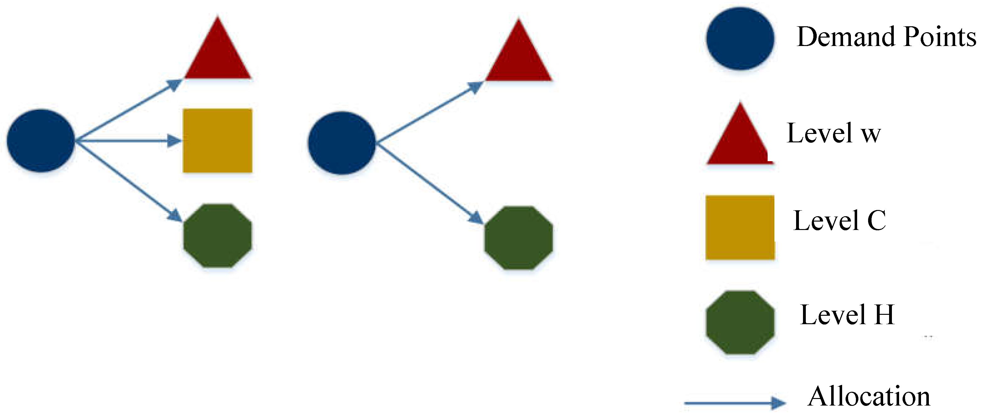
Figure 1.
Average of Averages Plot for NSGA II Algorithm.
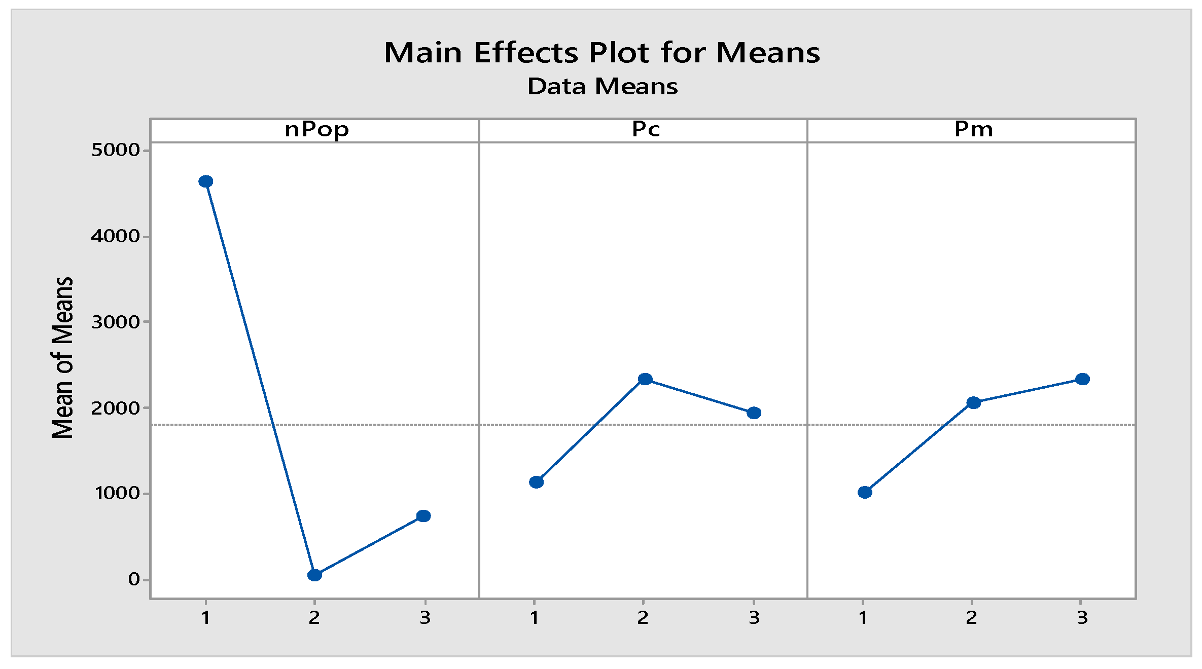
Figure 2.
Average S/N Ratio Plot for NSGA II Algorithm.
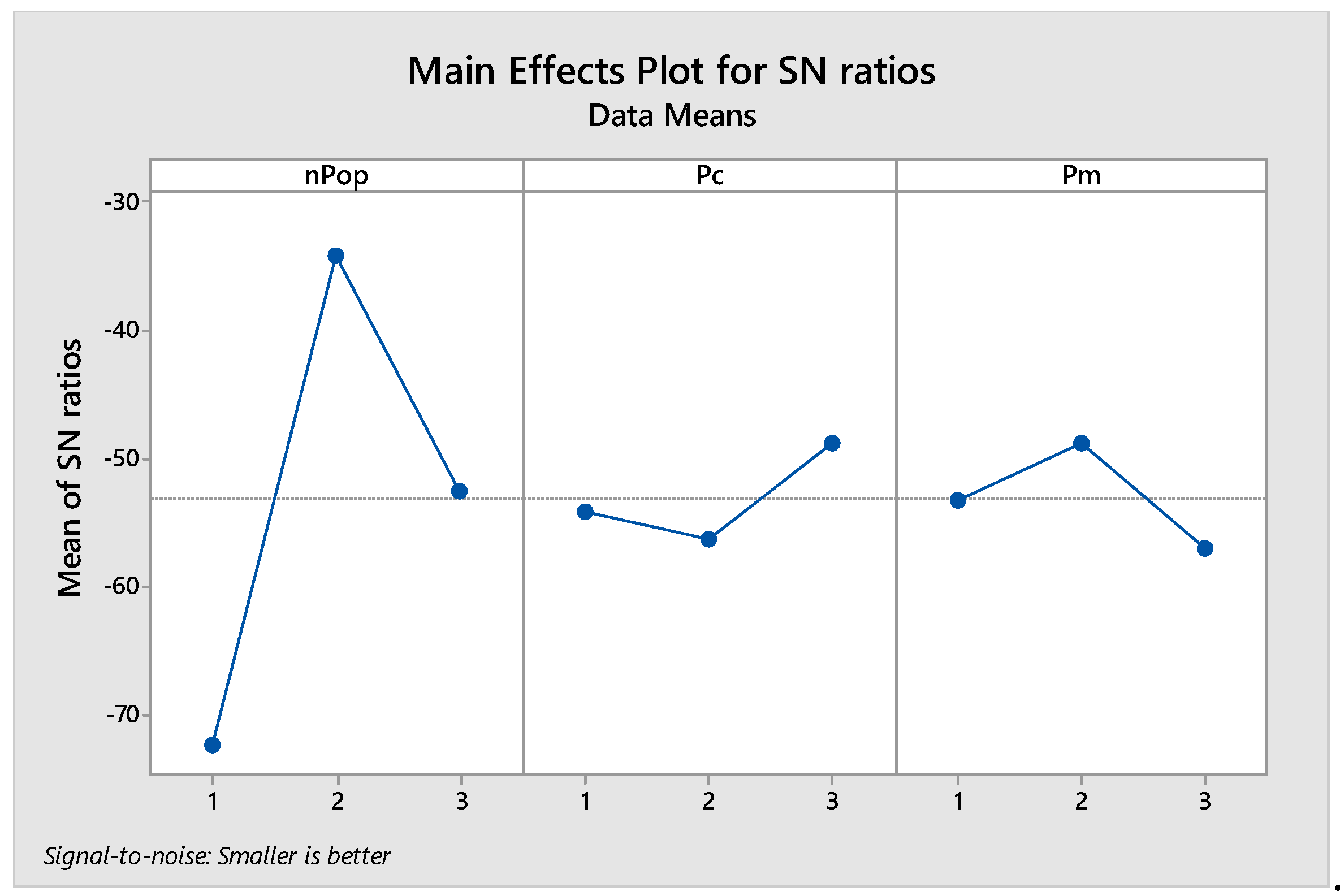
Figure 3.
Average Means Plot for the MOPSO Algorithm.
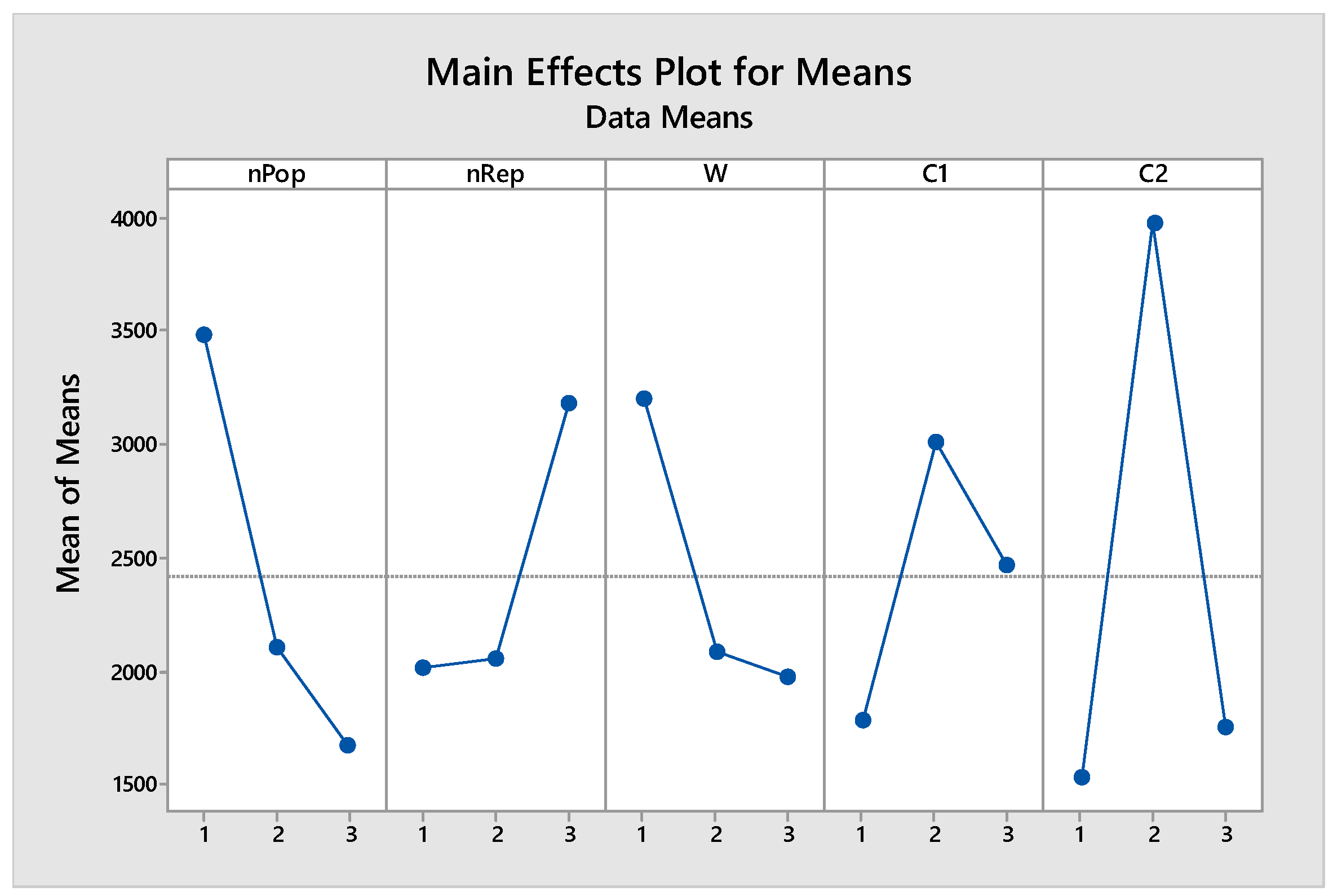
Figure 4.
Average S/N Ratio Plot for the MOPSO Algorithm.
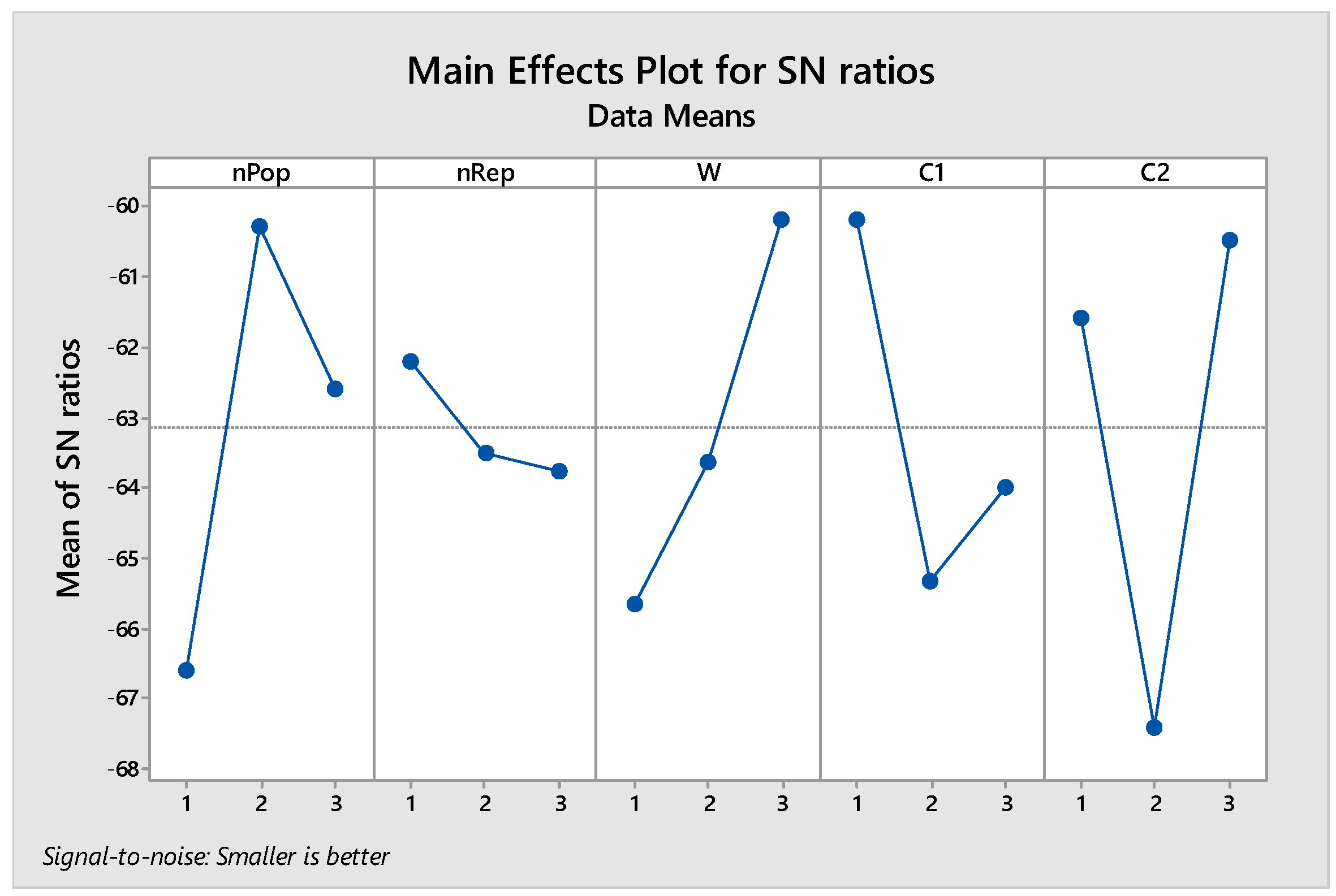
Figure 5.
Pareto Front obtained from solving the small-sized problem using NSGA II and MOPSO algorithms.
Figure 5.
Pareto Front obtained from solving the small-sized problem using NSGA II and MOPSO algorithms.
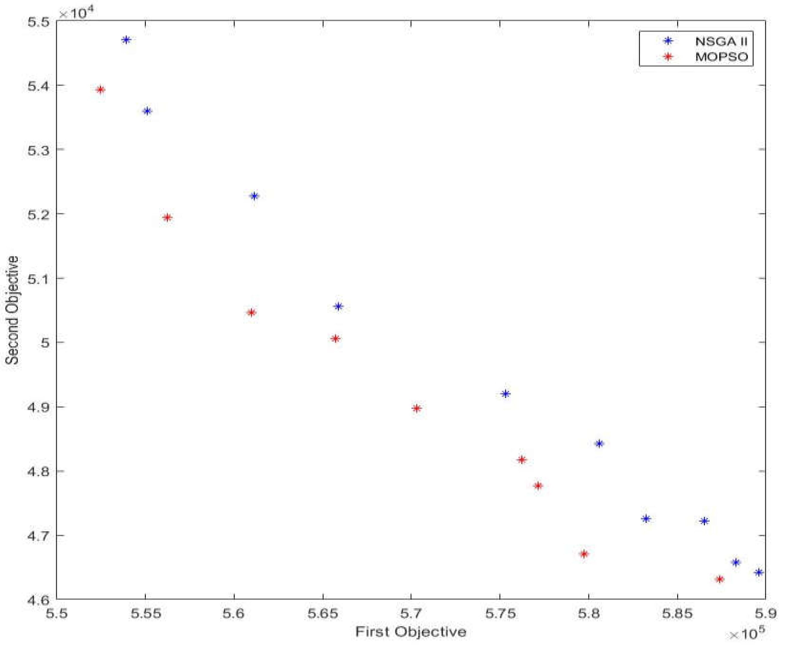
Figure 6.
Comparison of Mean Values of the First Objective Function in Sample Problems with Metaheuristic Algorithms.
Figure 6.
Comparison of Mean Values of the First Objective Function in Sample Problems with Metaheuristic Algorithms.
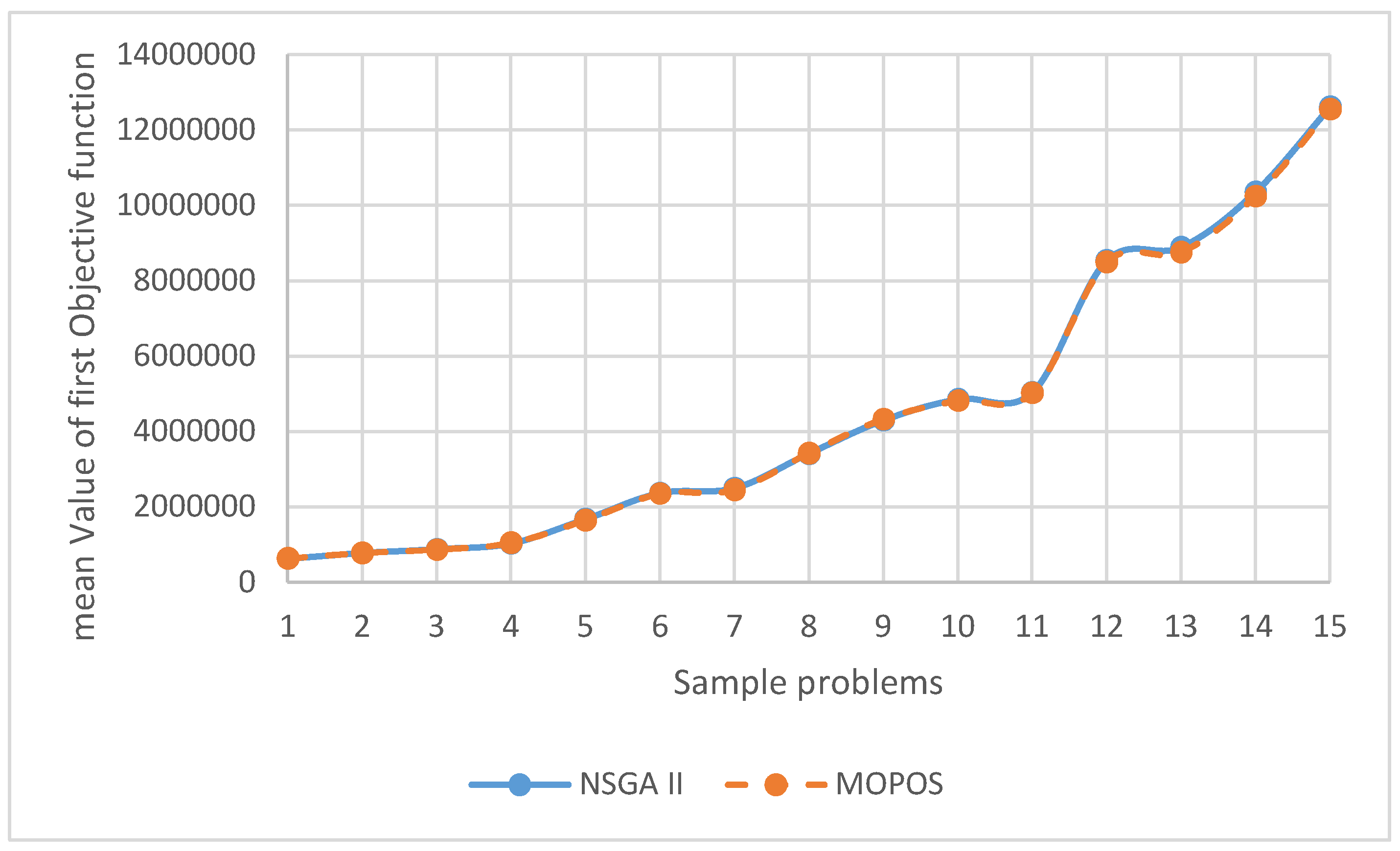
Figure 7.
Boxplot for confirming or rejecting the null hypothesis for the means of the first objective function.
Figure 7.
Boxplot for confirming or rejecting the null hypothesis for the means of the first objective function.
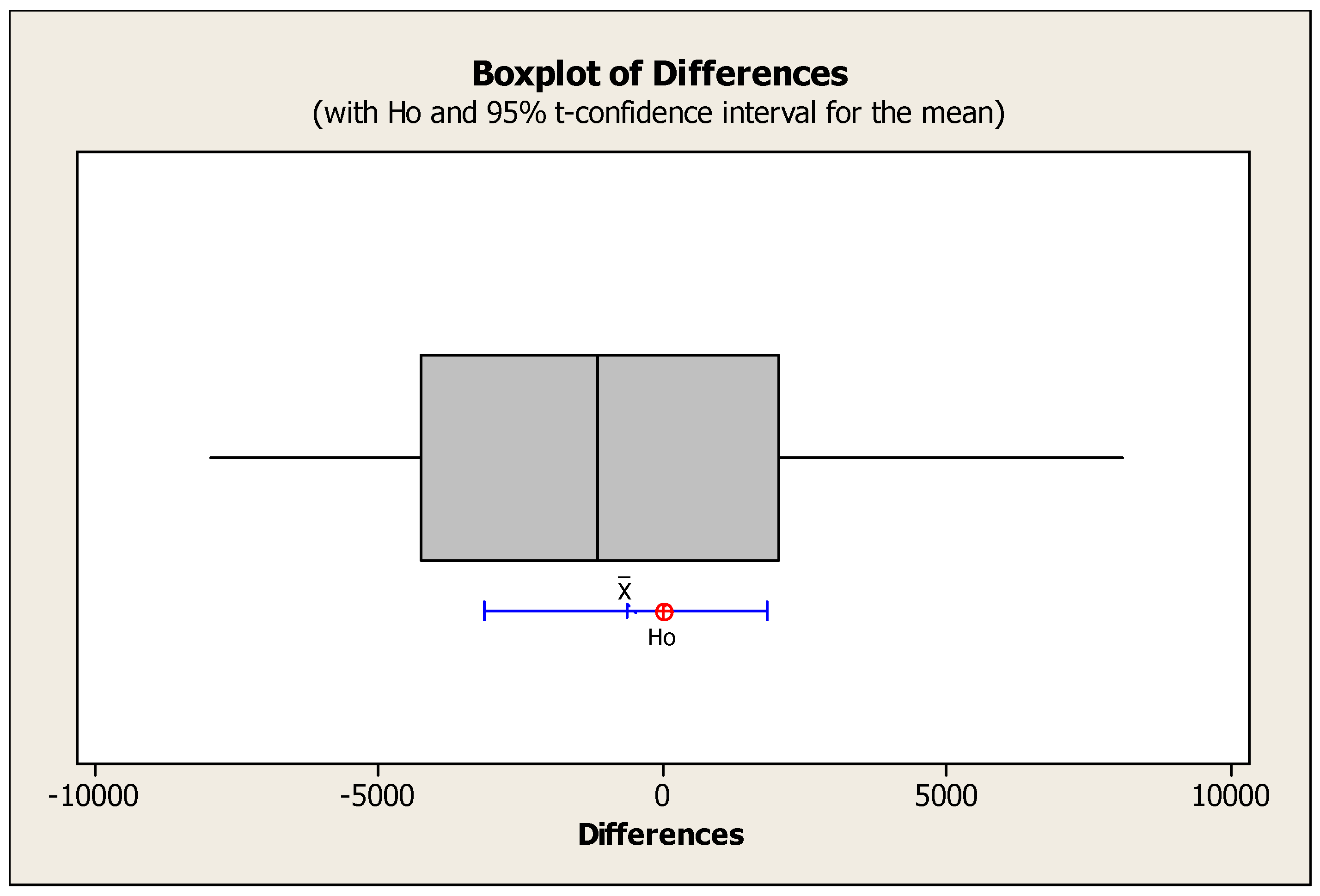
Figure 8.
Comparison of the mean values of the second objective function in sample problems using metaheuristic algorithms.
Figure 8.
Comparison of the mean values of the second objective function in sample problems using metaheuristic algorithms.
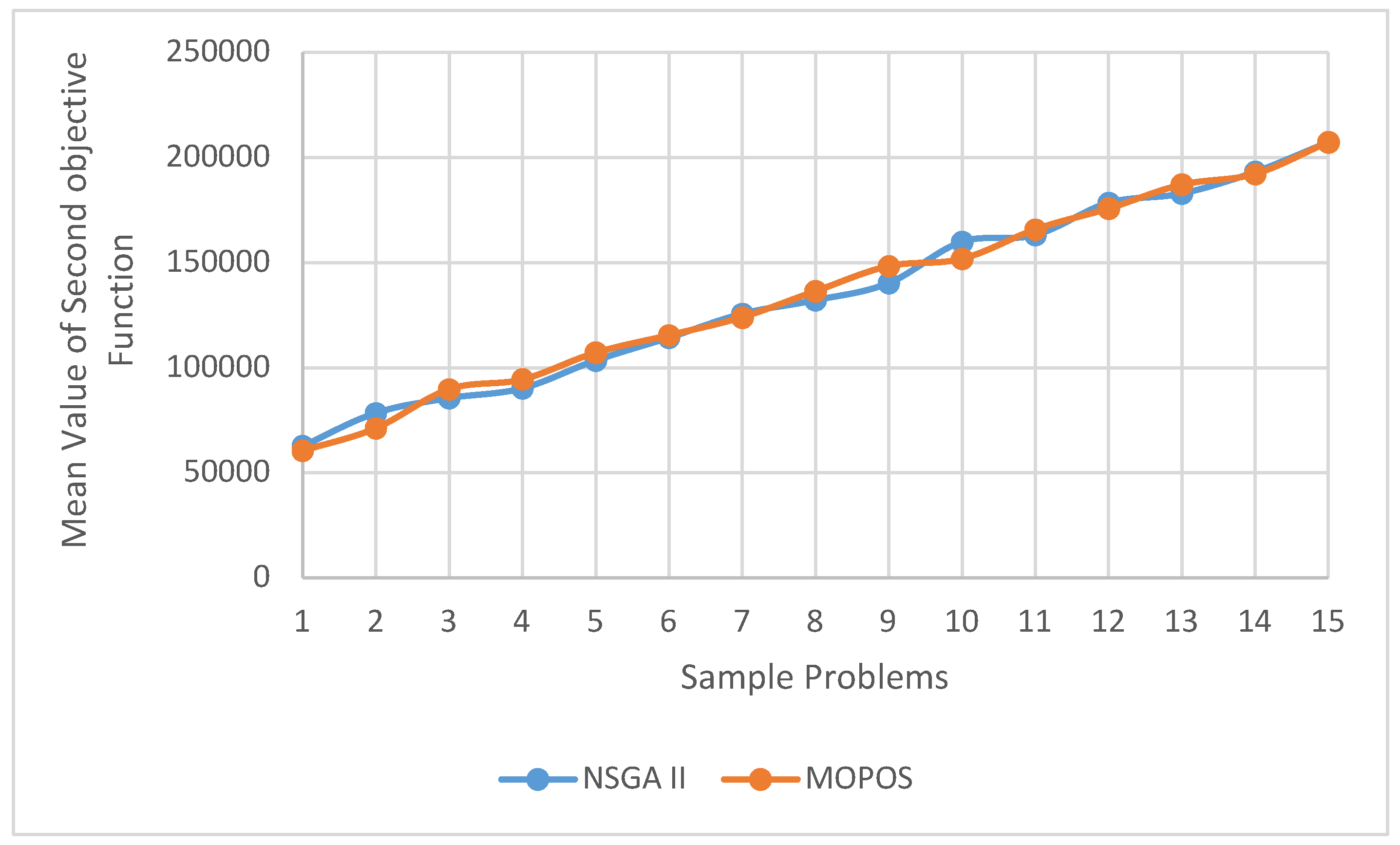
Figure 9.
illustrates the boxplot for confirming or rejecting the null hypothesis for the means of the second objective function.
Figure 9.
illustrates the boxplot for confirming or rejecting the null hypothesis for the means of the second objective function.
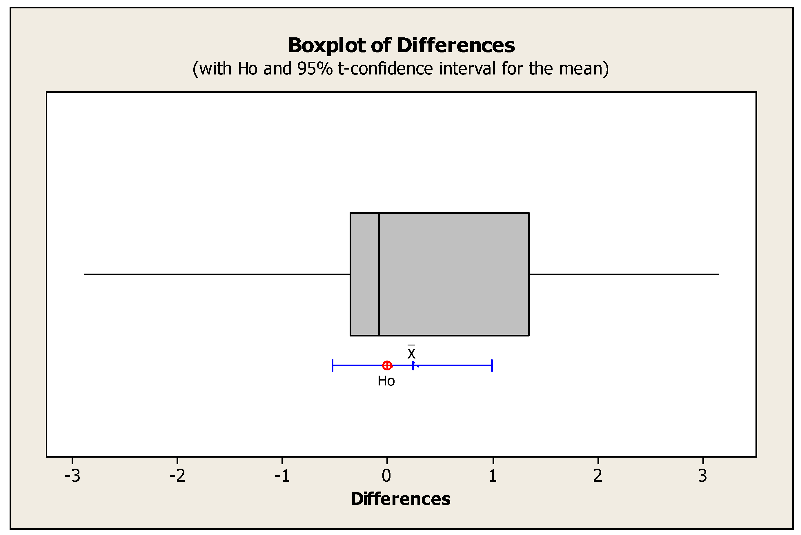
Figure 10.
Comparison of average number of efficient solutions in sample problems using metaheuristic algorithms.
Figure 10.
Comparison of average number of efficient solutions in sample problems using metaheuristic algorithms.
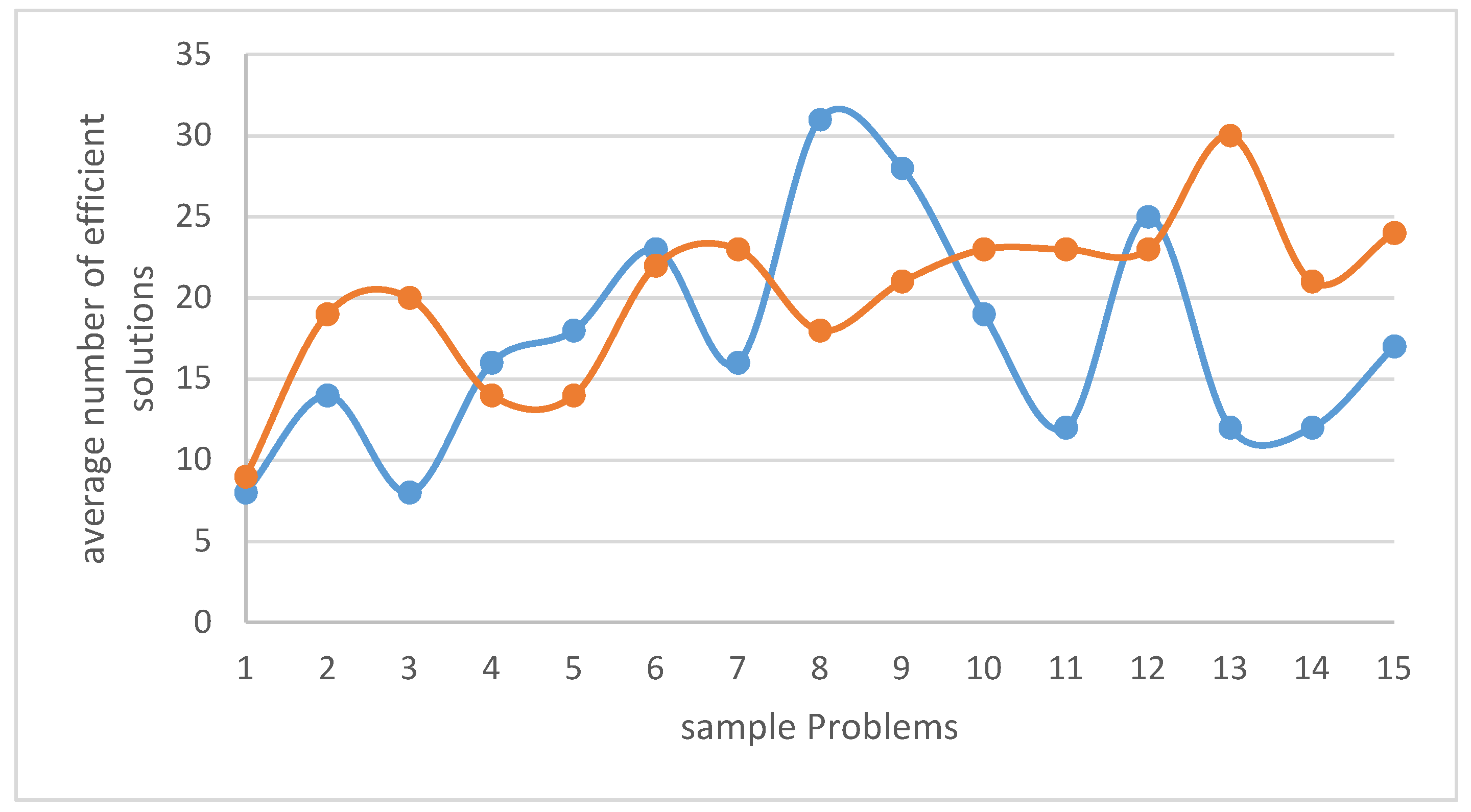
Figure 11.
Box plot to confirm or reject the null hypothesis for the averages of the number of efficient solutions.
Figure 11.
Box plot to confirm or reject the null hypothesis for the averages of the number of efficient solutions.
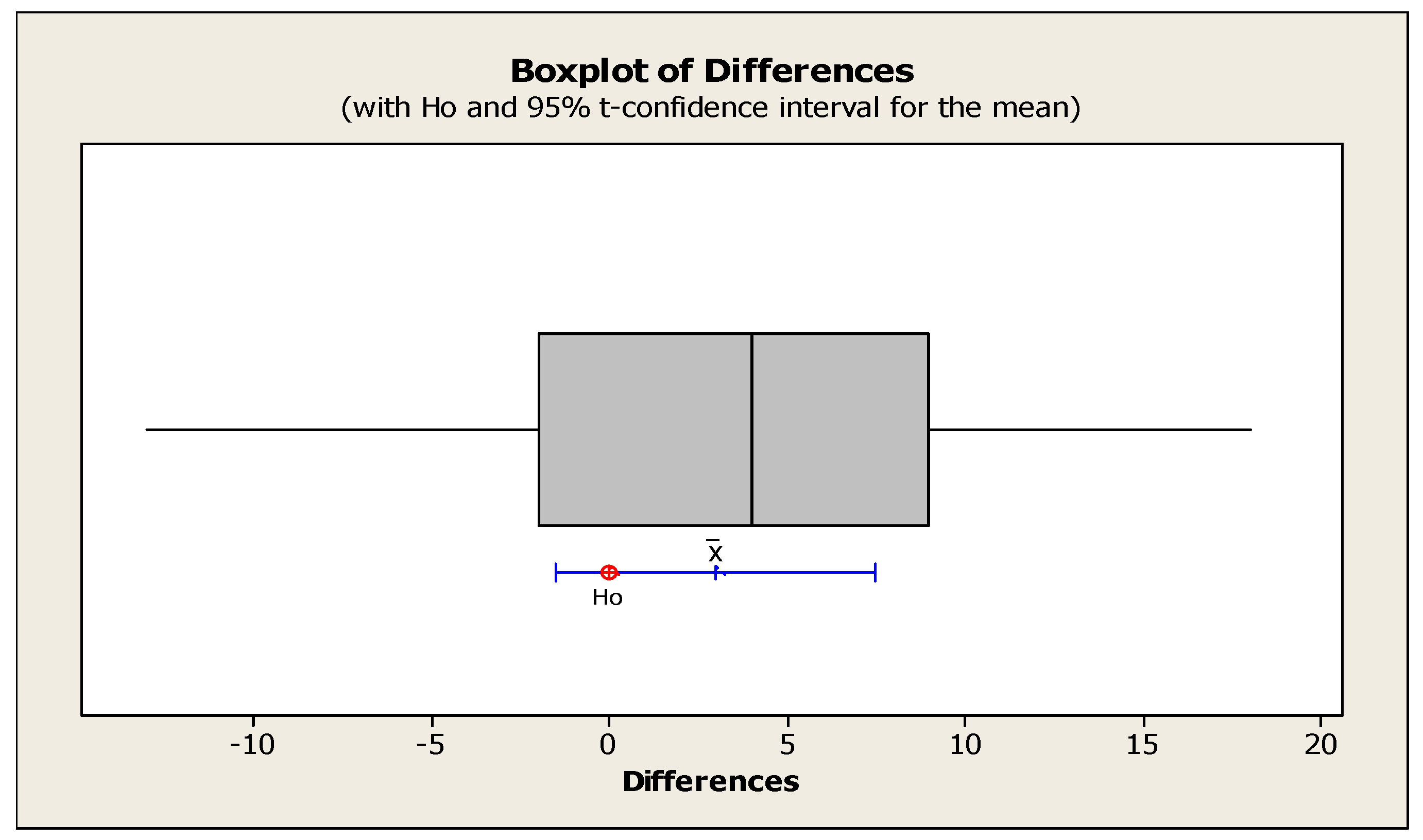
Figure 12.
Comparison of the means of the maximum spread indicator in sample problems with metaheuristic algorithms.
Figure 12.
Comparison of the means of the maximum spread indicator in sample problems with metaheuristic algorithms.

Figure 13.
Box plot to confirm or reject the null hypothesis for the means of the Maximum Spread Indicator.
Figure 13.
Box plot to confirm or reject the null hypothesis for the means of the Maximum Spread Indicator.
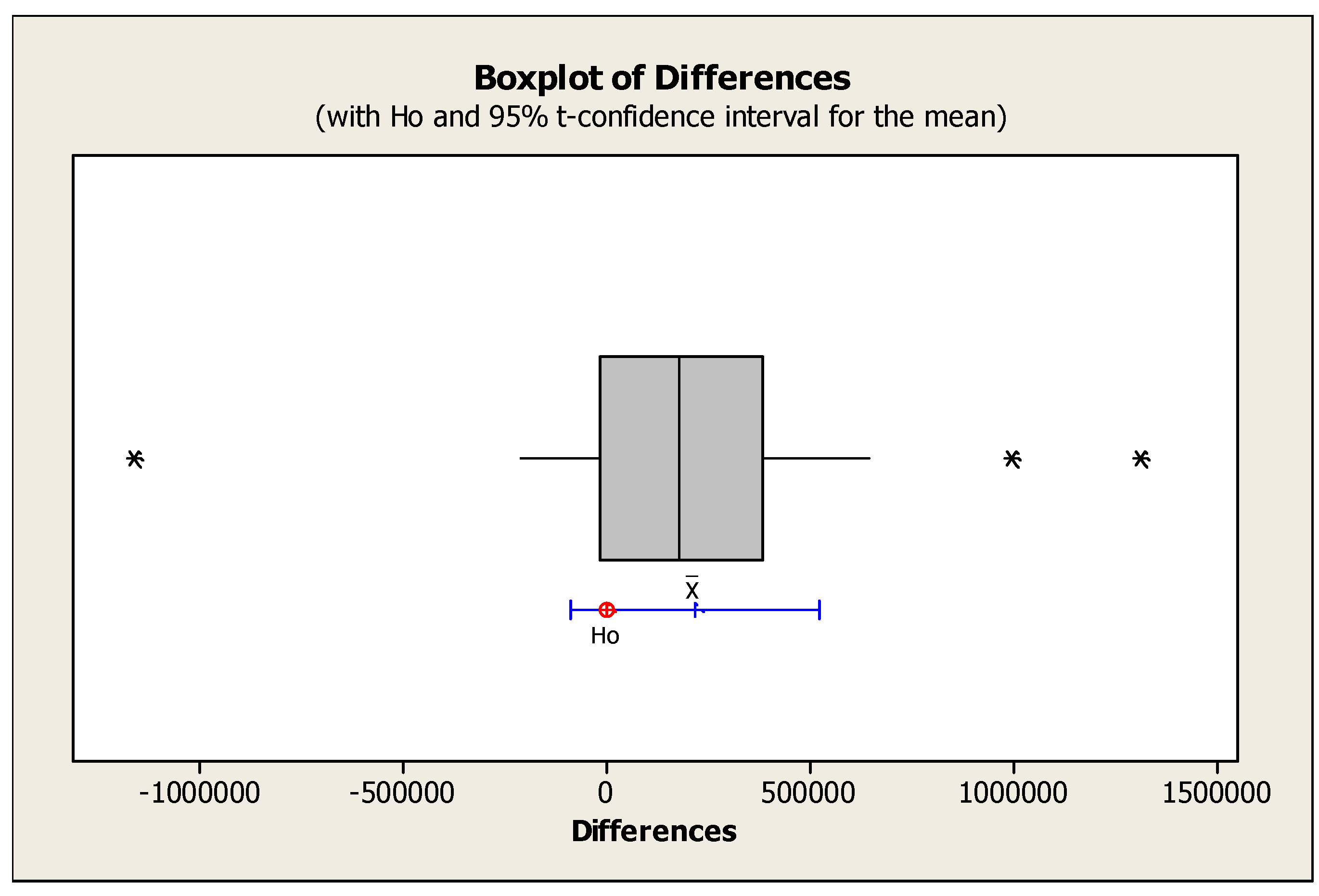
Figure 14.
Comparison of average spacing index in example problems with meta-heuristic algorithms.
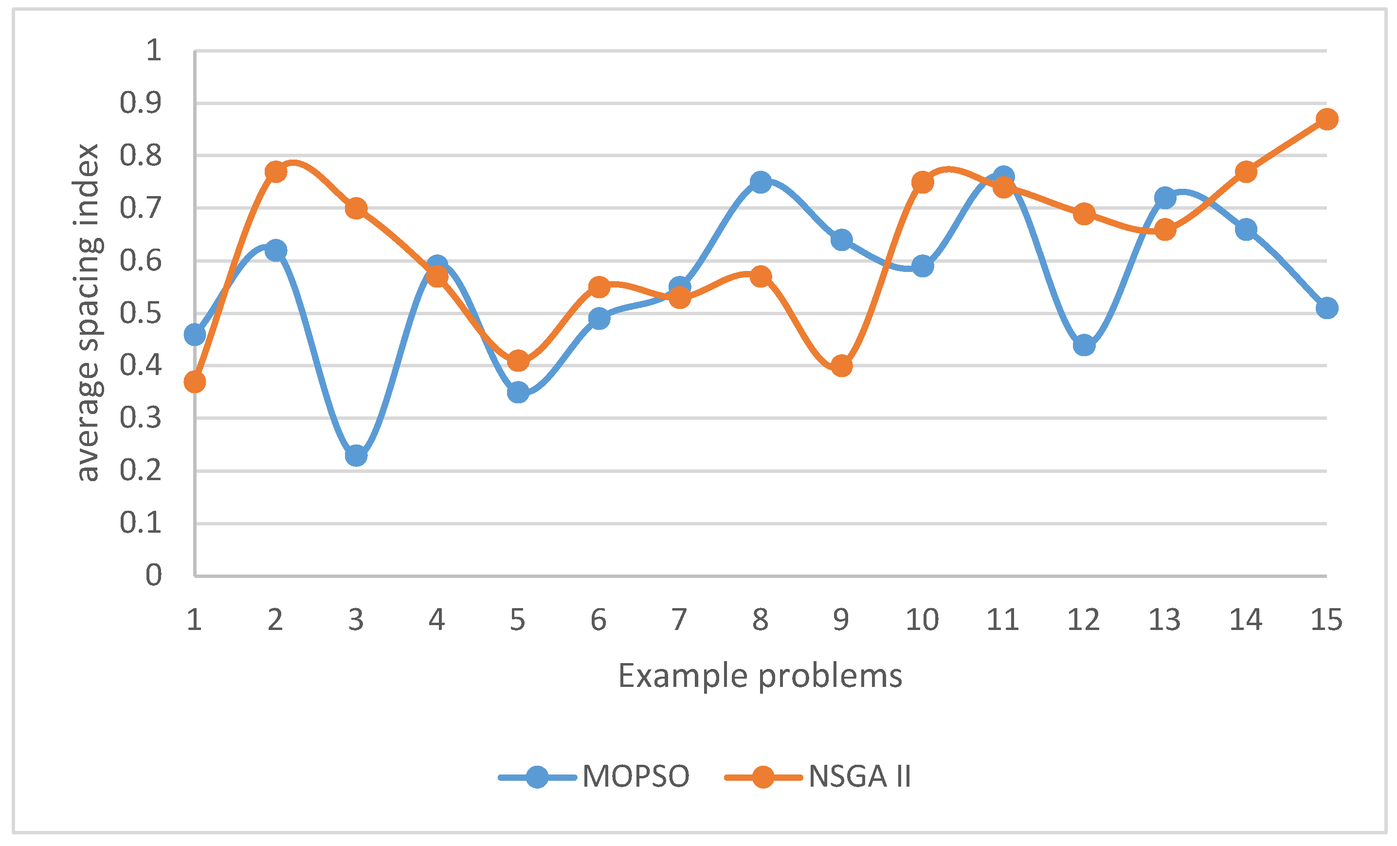
Figure 15.
Box plot to confirm or reject the null hypothesis for the averages of distance index.
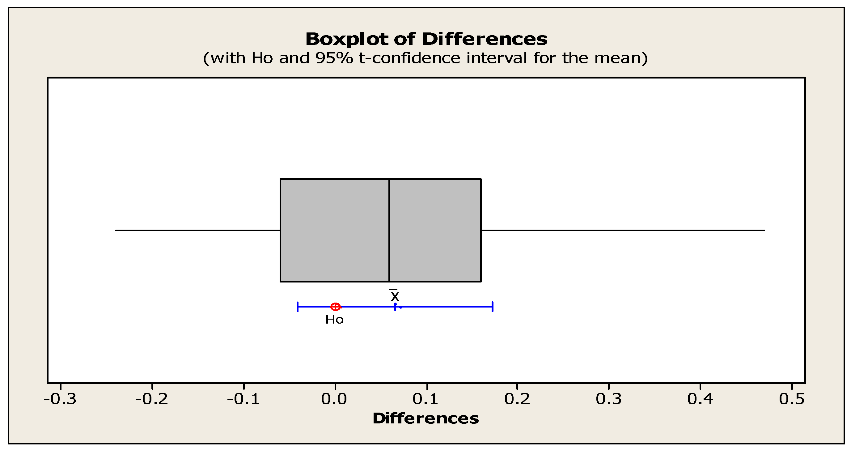
Figure 16.
Comparison of computing time averages in example problems with meta-heuristic algorithms.
Figure 16.
Comparison of computing time averages in example problems with meta-heuristic algorithms.
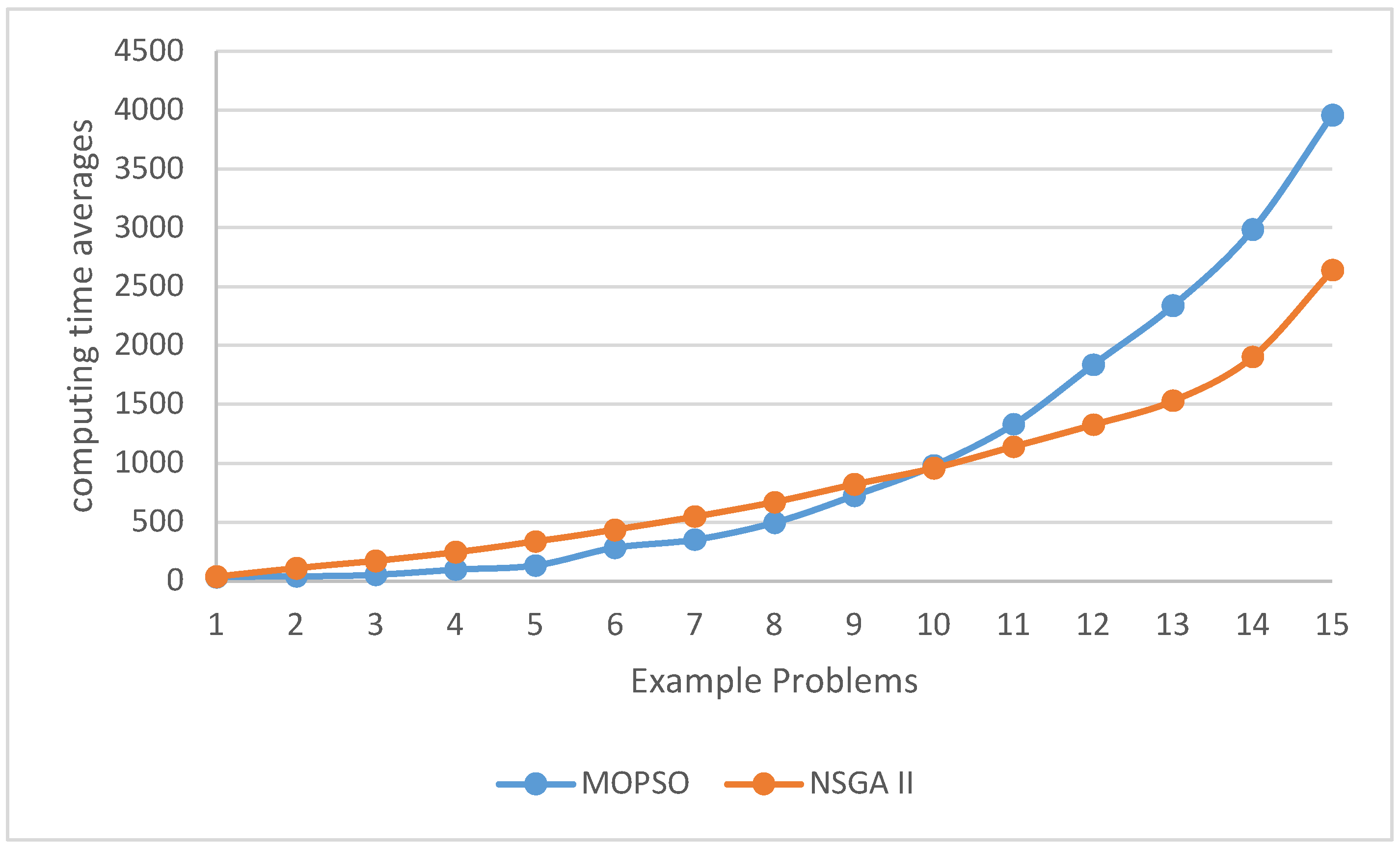
Figure 17.
Box plot for confirming or rejecting the null hypothesis for computing time averages.
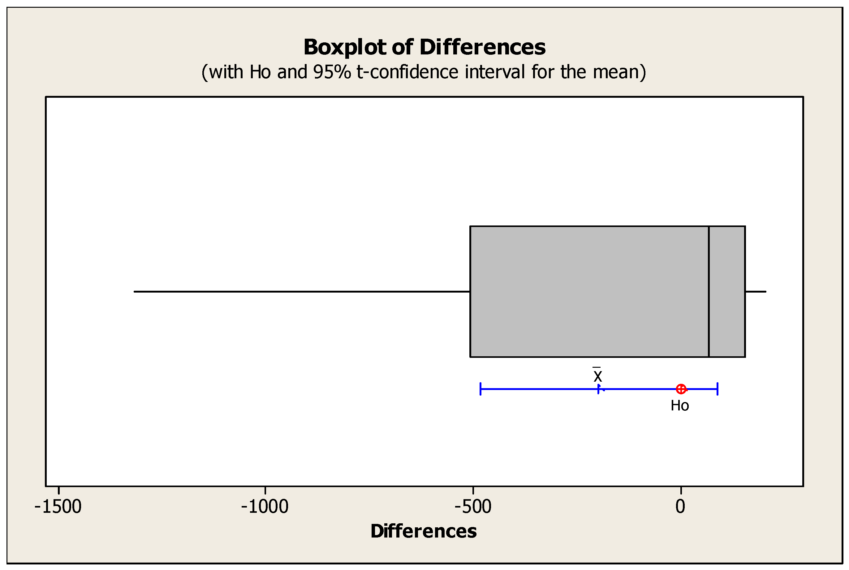
Table 1.
Levels of Factors Used for the NSGA-II Algorithm.
| Levels of Factors | |||
| Parameters | 1 | 2 | 3 |
| nPop | 50 | 70 | 100 |
| pc | 0.2 | 0.5 | 0.8 |
| pm | 0.2 | 0.3 | 0.4 |
Table 2.
Orthogonal Arrays L9(33) for NSGA-II Algorithm.
| Experiment number | nPop | Pc | Pm |
| 1 | 1 | 1 | 1 |
| 2 | 1 | 2 | 2 |
| 3 | 1 | 3 | 3 |
| 4 | 2 | 1 | 2 |
| 5 | 2 | 2 | 3 |
| 6 | 2 | 3 | 1 |
| 7 | 3 | 1 | 3 |
| 8 | 3 | 2 | 1 |
| 9 | 3 | 3 | 2 |
Table 3.
Levels of factors used for the MOPSO algorithm.
| Levels of factors | |||
| Parameters | 1 | 2 | 3 |
| nPop | 50 | 75 | 100 |
| nRep | 70 | 100 | 150 |
| W | 0.5 | 0.6 | 0.7 |
| C1 | 1 | 1.25 | 1.5 |
| C2 | 1 | 1.25 | 1.5 |
Table 4.
Orthogonal Arrays L9(35) for MOPSO Algorithm.
| C2 | C1 | W | nRep | nPop | Experiment Number |
| 1 | 1 | 1 | 1 | 1 | 1 |
| 2 | 1 | 1 | 1 | 1 | 2 |
| 3 | 1 | 1 | 1 | 1 | 3 |
| 1 | 2 | 2 | 2 | 1 | 4 |
| 2 | 2 | 2 | 2 | 1 | 5 |
| 3 | 2 | 2 | 2 | 1 | 6 |
| 1 | 3 | 3 | 3 | 1 | 7 |
| 2 | 3 | 3 | 3 | 1 | 8 |
| 3 | 3 | 3 | 3 | 1 | 9 |
| 1 | 1 | 1 | 1 | 2 | 10 |
| 2 | 1 | 1 | 1 | 2 | 11 |
| 3 | 1 | 1 | 1 | 2 | 12 |
| 1 | 2 | 2 | 2 | 2 | 13 |
| 2 | 2 | 2 | 2 | 2 | 14 |
| 3 | 2 | 2 | 2 | 2 | 15 |
| 1 | 3 | 3 | 3 | 2 | 16 |
| 2 | 3 | 3 | 3 | 2 | 17 |
| 3 | 3 | 3 | 3 | 2 | 18 |
| 1 | 1 | 1 | 1 | 3 | 19 |
| 2 | 1 | 1 | 1 | 3 | 20 |
| 3 | 1 | 1 | 1 | 3 | 21 |
| 1 | 2 | 2 | 2 | 3 | 22 |
| 2 | 2 | 2 | 2 | 3 | 23 |
| 3 | 2 | 2 | 2 | 3 | 24 |
| 1 | 3 | 3 | 3 | 3 | 25 |
| 2 | 3 | 3 | 3 | 3 | 26 |
| 3 | 3 | 3 | 3 | 3 | 27 |
Table 5.
Levels of Factors Used for MOPSO Algorithm.
| Optimal Level of Factors | Levels of Factors | |||
| 3 | 2 | 1 | Parameters | |
| 100 | 100 | 75 | 50 | nPop |
| 70 | 150 | 100 | 70 | nRep |
| 0.7 | 0.7 | 0.6 | 0.5 | W |
| 1 | 1.5 | 1.25 | 1 | C1 |
| 1 | 1.5 | 1.25 | 1 | C2 |
Table 6.
Comparison Metrics of Metaheuristic Algorithms in Solving the Sample Problem.
| MOPSO algorithm | NSGA-II algorithm | Index |
| 6.64 | 18.88 | Computational time |
| 569563.9 | 573954.2 | Average of the first objective function |
| 49371.86 | 49622.11 | Average of the second objective function |
| 9 | 10 | NPF |
| 35751.92 | 36643.3 | MSI |
| 0.381 | 0.476 | SM |
Table 7.
Size of sample problems in larger sizes.
| Sample problem | ||||
| 8 | 6 | 4 | 4 | 1 |
| 9 | 6 | 4 | 6 | 2 |
| 10 | 7 | 4 | 6 | 3 |
| 12 | 8 | 5 | 10 | 4 |
| 16 | 9 | 10 | 12 | 5 |
| 17 | 11 | 12 | 15 | 6 |
| 18 | 12 | 14 | 15 | 7 |
| 20 | 12 | 15 | 15 | 8 |
| 21 | 13 | 16 | 16 | 9 |
| 24 | 14 | 16 | 16 | 10 |
| 25 | 15 | 16 | 17 | 11 |
| 26 | 15 | 17 | 18 | 12 |
| 27 | 16 | 17 | 19 | 13 |
| 28 | 16 | 17 | 19 | 14 |
| 30 | 20 | 20 | 20 | 15 |
Table 8.
Average Objective Functions and Comparison Indices in Solving with NSGA II Algorithm.
| Sample problem | First Objective Functions | Sum of the Second and Third Objective Functions | Number of Feasible Solutions | Maximum Spread Indicator | Diversity Distance Indicator | Computational Time |
| 1 | 633806.72 | 62601.70 | 9 | 270273.91 | 0.37 | 36.46 |
| 2 | 778692.87 | 78381.54 | 19 | 585593.25 | 0.77 | 108.00 |
| 3 | 881581.31 | 85446.74 | 20 | 479316.63 | 0.7 | 170.30 |
| 4 | 1033814.58 | 90080.84 | 14 | 850298.87 | 0.57 | 242.53 |
| 5 | 1674913.50 | 103382.09 | 14 | 1129077.89 | 0.41 | 335.50 |
| 6 | 2369557.62 | 114251.75 | 22 | 1508175.51 | 0.55 | 434.40 |
| 7 | 2500890.63 | 125554.34 | 23 | 1797128.03 | 0.53 | 545.77 |
| 8 | 3416474.10 | 132080.49 | 18 | 2739770.14 | 0.57 | 669.07 |
| 9 | 4301935.98 | 140272.83 | 21 | 2529228.60 | 0.40 | 819.60 |
| 10 | 4860023.44 | 159821.22 | 23 | 3529017.44 | 0.75 | 959.67 |
| 11 | 5040590.70 | 163061.03 | 23 | 3087180.76 | 0.74 | 1040.13 |
| 12 | 8540218.42 | 178342.69 | 23 | 4883033.12 | 0.69 | 1326.00 |
| 13 | 8887924.17 | 182872.57 | 30 | 3839628.23 | 0.66 | 1528.37 |
| 14 | 10361985.83 | 193154.36 | 21 | 456422.62 | 0.77 | 1802.27 |
| 15 | 12608666.41 | 207290.80 | 24 | 538709.71 | 0.87 | 2640.00 |
Table 9.
Average Objective Functions and Comparison Metrics in Solving with MOPSO Algorithm.
| Sample problem | First Objective Functions | Sum of the Second and Third Objective Functions | Number of Feasible Solutions | Maximum Spread Indicator | Diversity Distance Indicator | Computational Time |
| 1 | 635858.69 | 60567.22 | 8 | 109850.13 | 0.46 | 34.40 |
| 2 | 776699.89 | 71074.60 | 14 | 329845.53 | 0.62 | 39.07 |
| 3 | 871134.25 | 89693.95 | 8 | 370471.43 | 0.23 | 51.66 |
| 4 | 1046187.49 | 94437.00 | 16 | 463108.57 | 0.59 | 95.93 |
| 5 | 1653146.41 | 107002.93 | 18 | 817523.73 | 0.35 | 131.20 |
| 6 | 2353344.22 | 115415.91 | 23 | 15261236.70 | 0.49 | 280.50 |
| 7 | 2450251.68 | 123910.36 | 16 | 2008648.76 | 0.55 | 349.16 |
| 8 | 3434001.90 | 136349.08 | 31 | 2559860.14 | 0.75 | 494.70 |
| 9 | 4334688.39 | 148225.98 | 28 | 3694417.30 | 0.64 | 723.16 |
| 10 | 4817592.14 | 151730.43 | 19 | 2215230.18 | 0.59 | 980.40 |
| 11 | 5020566.34 | 165792.57 | 12 | 2437807.90 | 0.76 | 1328.75 |
| 12 | 8500502.39 | 175673.57 | 25 | 3887334.58 | 0.44 | 1834.56 |
| 13 | 8759033.18 | 187113.32 | 12 | 3757576.19 | 0.72 | 2337.30 |
| 14 | 10251098.76 | 192138.59 | 12 | 4593286.90 | 0.66 | 2983.04 |
| 15 | 12554017.27 | 207281.68 | 17 | 5138916.08 | 0.51 | 3957.90 |
Table 10.
Results of the T-Test output on the means of the first objective function.
| Algorithm | Sample size | Mean | Standard deviation | 95% confidence interval | T-test statistic | P-value |
| NSGA II | 15 | 5626072 | 3852039 | (4041*53686) | 2.49 | 0.026 |
| MOPSO | 15 | 4497208 | 3821250 |
Table 11.
Output results of the T-Test on the means of the second objective function.
| Algorithm | Sample size | Mean | Standard deviation | 95% confidence interval | T-test statistic | P-value |
| NSGA II | 15 | 134440 | 45240 | (-3156*1848) | 0.56 | 0.584 |
| MOPSO | 15 | 135094 | 45418 |
Table 12.
Output Results of T-Test on the Means of Efficient Solutions.
| Algorithm | Sample size | Mean | Standard deviation | 95% confidence interval | T-test statistic | P-value |
| NSGA II | 15 | 20.27 | 5.04 | (-1.48*7.48) | 1.43 | 0.173 |
| MOPSO | 15 | 17.27 | 6.91 |
Table 13.
Results of T-Test on the Means of the Maximum Spread Indicator.
| Algorithm | Sample size | Mean | Standard deviation | 95% confidence interval | T-test statistic | P-value |
| NSGA II | 15 | 2478417 | 1496766 | (-88459*523960) | 1.53 | 0.149 |
| MOPSO | 15 | 2260667 | 1661211 |
Table 14.
Output results of the T-Test test on average spacing index.
| Algorithm | Sample size | Mean | Standard deviation | 95% confidence interval | T-test statistic | P-value |
| NSGA II | 15 | 0.623 | 0.152 | (-0.0405*0.1725) | 1.33 | 0.205 |
| MOPSO | 15 | 0.557 | 0.148 |
Table 15.
Output results of the T-Test test on average computing time.
| Algorithm | Sample size | Mean | Standard deviation | 95% confidence interval | T-test statistic | P-value |
| NSGA II | 15 | 844 | 730 | (-483*88) | 1.48 | 0.160 |
| MOPSO | 15 | 1041 | 1220 |
Table 16.
Overview of the significant difference between the average comparison indicators.
| index | A significant difference between the averages of the indicators |
| Computational time | Yes |
| Average of the first objective function | No |
| Average of the second objective function | No |
| NPF | No |
| MSI | No |
| SM | No |
Table 17.
Average indices obtained from meta-heuristic algorithms.
| Algorithm | First Objective Functions | Sum of the Second and Third Objective Functions | Number of Feasible Solutions | Maximum Spread Indicator | Diversity Distance Indicator | Computational Time |
| NSGA II | 4526072 | 45240 | 20.27 | 2478417 | 0.623 | 844 |
| MOPSO | 4497208 | 45418 | 17.27 | 2260667 | 0.557 | 1041 |
| Weight | 0.4 | 0.4 | 0.05 | 0.05 | 0.05 | 0.05 |
Disclaimer/Publisher’s Note: The statements, opinions and data contained in all publications are solely those of the individual author(s) and contributor(s) and not of MDPI and/or the editor(s). MDPI and/or the editor(s) disclaim responsibility for any injury to people or property resulting from any ideas, methods, instructions or products referred to in the content. |
© 2024 by the authors. Licensee MDPI, Basel, Switzerland. This article is an open access article distributed under the terms and conditions of the Creative Commons Attribution (CC BY) license (http://creativecommons.org/licenses/by/4.0/).
Copyright: This open access article is published under a Creative Commons CC BY 4.0 license, which permit the free download, distribution, and reuse, provided that the author and preprint are cited in any reuse.


