Submitted:
23 October 2024
Posted:
24 October 2024
You are already at the latest version
Abstract
Reliable fault detection in satellite attitude control systems stands as a critical aspect of ensuring the safety and success of space missions. Central to these systems, Reaction Wheels (RWs), despite being the most frequently used actuators, present a vulnerability given their susceptibility to faults - a factor with the potential to precipitate catastrophic failures such as total satellite loss. In light of this, we introduce a fault detection methodology grounded in deep learning techniques specifically designed for satellite attitude control systems. Our proposed method utilizes a Long Short-Term Memory (LSTM) model adept at learning temporal patterns inherent to both healthy and faulty system behaviors. Incorporated into our model is a torque allocation algorithm designed to circumnavigate specific velocities known to induce torque disturbances, a factor known to influence LSTM performance adversely. To bolster the robustness of our fault detection technique, we also incorporate denoising autoencoders within the LSTM framework, thereby enabling the model to identify temporal patterns in healthy and faulty system behavior, even amidst the noise. Extensive evaluation of our proposed method on a simulated satellite attitude control system affirmed its ability to achieve commendable fault detection accuracy, demonstrating high system reliability and robustness to noisy input data. Our research underscores a stride in the evolution of fault detection and control strategies for satellite attitude control systems, holding promise to boost the reliability and efficiency of future space missions.
Keywords:
Reaction Wheel
; Long Short-Term Memory (LSTM)
; Deep learning
; Fault detection
; Attitude control systems
1. Introduction
Satellites, fundamental to a broad spectrum of applications from scientific observations to communication and navigation, require fast and accurate attitude control for optimal performance in three-axis. One of the main mechanisms employed to supply this control torque are Reaction Wheels (RWs), underscoring the importance of their reliability and accuracy for the success of space missions. Consequently, the need for robust RWs’ fault diagnosis and prognosis is critical. This foregrounds the urgent requirement for improved fault detection and mitigation strategies in RWs [1]. In recent years, the application of deep learning techniques for fault detection and control in satellite attitude control systems has been recognized as a promising solution. It offers the capability to effectively analyze complex, high-dimensional data, facilitating faster and more accurate fault detection and reducing the need for human intervention [2]. Thus, it significantly enhances mission success rate while minimizing mission risks. This paper presents an approach for fault detection in satellite attitude control systems focusing on RWs. We propose a method based on Long Short-Term Memory (LSTM)-driven deep learning, which capitalizes on LSTM's proficiency in handling time-series data, complemented by advanced torque allocation algorithms and denoising autoencoders to mitigate false alarms. By detecting subtle temporal changes in system behavior, our approach improves fault detection accuracy and enhances system reliability and performance.
Satellite attitude control systems encompass diverse components: sensors, actuators, and controllers. The function of the sensors is to gauge the spacecraft's attitude relative to a reference framework. Actuators, on the other hand, generate the force needed to modify the spacecraft's position or attitude respectively. Controllers get sensor data and ascertain the appropriate corrective actions to stabilize or alter the spacecraft's attitude. Common actuators in satellite attitude control systems are Control Moment Gyroscopes (CMGs) and Reaction Wheels (RWs) [2,3,4]. RWs are rotational instruments used in satellites to yield control torques for precise spacecraft alignment. Devices of this kind generate twisting forces by altering the rotational inertia of a flywheel. This is made possible through an electric motor and is attached to the framework of the space vehicle through a bearing mechanism. To provide a backup for orientation control in case of wheel failure, numerous spacecraft are equipped with an assembly of multiple Reaction Wheels (RWs), often more than three, arranged in a non-planar configuration, known as a Reaction Wheel Assembly (RWA). Strategies for torque mapping are utilized to apportion the necessary control torques to the RWs in a non-unique fashion [5]. Various methods for torque mapping have been suggested, such as the pseudo-inverse method [6,7,8], which aims to minimize a specific norm of the apportioned RW torques, and the L∞-norm method [9,10,11], which strives to minimize the highest RW torque in the RWA for a given slew maneuver [12]. Satellite reaction wheel fault detection is dependent on torque allocation algorithms because these algorithms ensure the optimal distribution of torque to reaction wheels, which directly affects their performance and reliability. Any anomalies in the allocated torque can indicate potential faults or impending failures in the reaction wheels, thereby making the torque allocation algorithm a component of the fault detection process [2,13].
In recent years, several methods for reaction wheel fault detection have been proposed [14,15,16]. These approaches include model-based methods and data-driven methods. Model-based methods rely on mathematical models of the satellite and reaction wheel dynamics to detect faults [17]. One such method was proposed by Rahimi et al. [18], who introduced an innovative approach for the detection of RWs malfunctions in satellite attitude control systems, utilizing an adaptive unscented Kalman filter that models the RWs’ dynamics. Model-based fault detection faces challenges in accurately capturing complex system dynamics and handling uncertainties, which can result in reduced sensitivity to faults and increased false alarms. Accordingly, data-driven methods are receiving more attention during the recent years. Data-driven methods utilize machine learning algorithms and statistical methods to identify faults based on historical or real-time data. For example, Ibrahim et al. [19] proposed a fault detection method using support vector machines, while Abd-Elhay et al. employed a deep learning-based approach for reaction wheel fault diagnosis [16]. Data-driven fault detection can also struggle with limited or noisy data, which can impede learning accuracy.
Addressing the aforementioned challenges, deep learning techniques have recently demonstrated promising results in diverse fault detection applications, exhibiting enhanced accuracy and efficiency compared to traditional methodologies. Convolutional Neural Networks (CNNs) have been applied to image-based fault detection [20], while Recurrent Neural Networks (RNNs), specifically Long Short-Term Memory (LSTMs), have been utilized for time-series data fault detection [8]. LSTMs, a subclass of RNNs, have proven effective in managing long-term dependencies and complex temporal patterns, rendering them suitable for fault detection and control in satellite attitude control systems where learning temporal relationships is crucial [20,21]. LSTM is a type of recurrent neural network (RNN) that is commonly used for analysis of time-series data, including fault detection in industrial processes [22]. In fault detection applications, LSTM can be trained on historical sensor data from a machine or industrial process to learn patterns of normal behavior. The LSTM model can then be used to predict the expected sensor readings at each time step based on the previous readings. During operation, if the sensor readings deviate significantly from the LSTM's predictions, it may indicate the presence of a fault or anomaly. The LSTM can be used to generate an alarm or trigger a maintenance action. The LSTM can also be used in conjunction with other machine learning techniques, such as clustering and outlier detection, to improve the accuracy of fault detection. For example, the LSTM can be used to identify time periods where the sensor readings are abnormal, and clustering algorithms can be used to group the abnormal periods into different fault types.
Although LSTM can perform well for fault detection, LSTM networks are often sensitive to the presence of noise and outliers in the input data, which can negatively impact their performance in fault detection tasks [23,24]. The robustness of LSTM networks to noisy input data remains a significant area of concern, especially in satellite attitude control systems where signal corruption may occur due to various sources such as sensor noise, cosmic radiation, and communication channel disruptions. In this study, we propose a methodology for mitigating reaction wheel (RW) disturbances in satellite attitude control systems through the implementation of an effective torque allocation algorithm. This algorithm capitalizes on redundant RWs to circumvent particular velocities that may generate torque perturbations, such as zero-speed crossings and resonant speeds. Furthermore, our research endeavors to establish a robust, a LSTM-based deep learning technique for fault detection in satellite attitude control systems, utilizing signals from the aforementioned redundant RWs, which evade specific speed-induced torque disturbances, and thereby enhanced LSTM accuracy. Hence, the present investigation aims to address the constraints of prior methodologies, delivering a more precise and efficient solution for fault detection and management in satellite attitude control systems. In addition, we integrate denoising autoencoders within the LSTM architecture to ensure the optimal performance and robustness of the proposed LSTM-based fault detection approach.
To tackle issues related to RWs speeds and torque disturbances which degrades LSTM’s efficiency, different algorithms, such as constrained PID controllers and null space torque components have been put forward [5]. Reckdahl [25] utilized a PID mechanism to steer wheel velocities to set benchmarks, with an objective to lengthen the periods between back-to-back momentum offload activities. Modifications to improve upon Reckdahl's initial technique were suggested by both Ratan and Li [26] and Kron and colleagues [27]. These strategies mainly zeroed in on general metrics of reaction wheel performance, including energy usage, torque forces, and momentum holding capacity. However, none of these methods explored ways to dodge specific problematic wheel speeds, like zero speed that can cause static friction issues. Rigger [28] introduced a real-time computational model that effectively keeps the wheel speeds away from near-zero regions, thereby mitigating static friction. However, this solution springs into action only when the wheel velocity exceeds a certain minimum, making its efficacy uncertain, especially during sequences of operations where subsequent shifts start from the concluding speeds of the prior movement. Leve and team [29] scrutinized diverse setups of momentum retention systems, notably control moment gyroscopes, to gauge their impact on spacecraft steerability. They considered wheel alignment for the management of singularities and optimizing energy reserves, but they didn't focus on particular wheel speed paths designed to minimize torque irregularities. In this project, we employ the Null Space Torque Algorithm, leveraging redundant reaction wheels to pre-empt common disturbances. This method reduced attitude controllers' settling time by around 40% compared to traditional techniques and it showcases the interplay between reaction wheel redundancy and configuration design, leading to an agile spacecraft. Using this algorithm enhances both fault tolerance and spacecraft agility, ultimately boosting the data collection rate and overall mission value [5].
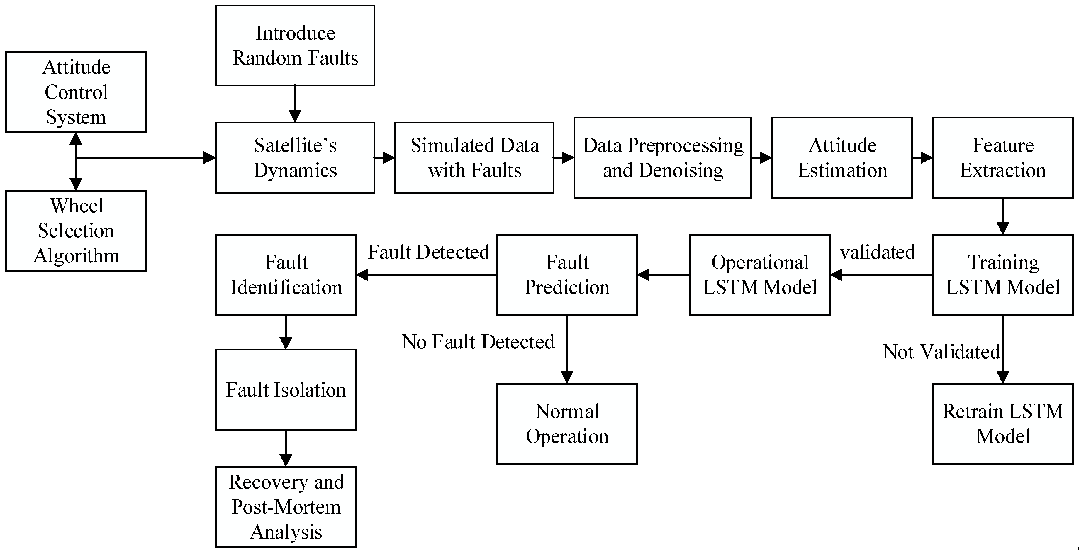
Error! Reference source not found. depicts the overall framework of our proposed algorithm. We provide a detailed description of the algorithm's flowchart, exploring its intricacies. In Section 1, we describe the dynamics of a spacecraft with faulty reaction wheels, highlighting associated challenges and characteristics. Section 2 outlines the design and operation of the attitude control system, emphasizing its role in maintaining orientation. The core of our algorithm, presented in Section 3, comprises an LSTM network tailored for fault detection in satellite systems. We explain the network's structure and training methodology, emphasizing its effectiveness in detecting faults. Section 5 showcases numerical tests and results, evaluating the algorithm's fault detection performance. We discuss findings, conduct a comprehensive analysis, and address limitations and potential improvements. In the concluding remarks (Section 6), we summarize our research's key contributions and implications.
Figure 1.
Schematic of the proposed LSTM-based fault detection method for a satellite with redundant reaction wheels.
Figure 1.
Schematic of the proposed LSTM-based fault detection method for a satellite with redundant reaction wheels.
2. Dynamics of the Spacecraft with faulty Reaction Wheel
In order to simulate the dynamics of a spacecraft with faulty reaction wheels, firstly we introduce the attitude dynamics of a spacecraft that uses a Reaction Wheel Assembly (RWA) for control torques. Such a dynamic model can be described in the rotating body frame. The governing equation for the attitude dynamics is as follows:
where:
is the inertia tensor of the spacecraft
- is the representation of the body-rate vector the body frame
- is the disturbance torque vector acting on the spacecraft in the body frame
- is the reaction wheels’ angular momentum vector in the body frame
- is the torque from the reaction wheels
Reaction wheels’ angular momentum vector in the body frame, , can be expressed as:
where:
is the reaction wheels’ configuration matrix, and is their inertia tensor in the reaction wheel frame, is the wheel speed vector for the entire RWA, represented in the reaction wheel frame, the inertia tensor and wheel speed vector can be written as:
and
These disturbance torques are modeled according to a referenced study [30]. The attitude dynamics Eq. (1) and the RWA angular momentum Eq. (2) together provide a comprehensive representation of the spacecraft's attitude dynamics in the presence of an RWA. This understanding is crucial for designing effective control strategies and ensuring accurate spacecraft orientation and stabilization.
2.1. Faulty Reaction Wheel’s Mathematical Model
Having the general spacecraft attitude equation as in Eq. (1), we can introduce reaction wheel faults into the dynamics model of the spacecraft with a Reaction Wheel Assembly (RWA). In this section we formulate a model of an RW by taking into account its bearings as well as the motor. The RW torque originates from the motor torque and is influenced by disturbances such as static friction , rotor mass imbalance-induced resonance and viscous bearing friction . The following subsections elaborate on the torque models.
2.2. Motor’s Numerical Model and Fault Scenarios
The Reaction Wheel (RW) receives its input twisting forces from an electric motor, where the motor's torque has a linear relationship with the electrical current, denoted as 'i'. The mathematical representation of the electric motor can be articulated as follows:
In this equation, and stand for the constants related to torque and counter-electromotive force, respectively. I and L correspond to the electrical resistance and inductance associated with the motor coils, respectively. V indicates the voltage input directed towards the motor coils. Within the context of this model, we aim to explore three distinct categories of malfunctions, which will be presented in this study:
Reaction Wheel Stiction
(1) The RW stiction arises from the static friction torque of the bearing, which consistently opposes the wheel speed direction. This stiction can result in significant tracking errors when the rotor alters its direction, causing an instantaneous change in the stiction direction. The stiction can be modeled by the following equation:
where defines the stiction magnitude.
Fault Scenario: The stiction magnitude in a faulty reaction wheel may change in several ways. In this study, we assume there is increased friction within the wheel's bearings or other mechanical components, which increases the stiction magnitude. This could be caused by worn-out or damaged bearings, misalignment, or inadequate lubrication.
Reaction Wheel Resonance
(2) Jitter is the term used for vibrational disturbances usually from a mass imbalance of a spinning RW. The jitter-induced resonance torque can be formulated as:
where defines the jitter amplitude, and h is the resonance number and is a random phase within the range . Additionally, represents the wheel speed at resonance, and is amplification factor due to structural resonance, which we assume to be the maximum according to [31].
Fault scenario: we assume excessive vibration, characterized by increased . It could be due to an imbalance in the wheel, a worn-out bearing, or a software issue causing the wheel to spin at an inappropriate speed. The vibration results in jitter, which could interfere with sensitive instruments or equipment onboard the spacecraft, possibly leading to failure.
(3) Viscous Friction-based Fault
The Torque induced by viscous friction of a reaction wheel opposes the wheel speed, with its magnitude being proportional to the wheel speed:
where is a constant to be calculated or given.
Fault scenario: We assume there is an increase in the viscous friction within the reaction wheel assembly due to a problem such as degraded lubrication or wear and tear in the bearings. This would be represented by an increase in the value of , which is typically constant in normal conditions. As increases, the opposing torque also increases for a given wheel speed . This increase in viscous friction causes the reaction wheel to consume more power in order to maintain the same wheel speed, potentially draining the spacecraft's power reserves faster than expected. This can also generate excess heat, which could damage the wheel itself or other nearby components if not properly dissipated. Moreover, the increased torque due to viscous friction could also make the RW less responsive to control inputs, thereby affecting the spacecraft's ability to maintain its desired attitude. Specifically, the spacecraft might start to drift from its desired orientation or fail to accurately point its instruments at its targets. If the lubrication issue or bearing wear worsens, the wheel might eventually seize or fail, which could lead to a loss of attitude control in the spacecraft, potentially causing mission failure.
2.3. Null Space Algorithm
In this document, we discuss how issues like stiction and resonance in reaction wheels (RWs) are closely related to the rotational speed of the wheels. By carefully planning the speed profile for each wheel, one can steer clear of problematic speeds, specifically zero speed and the resonance velocity. We employ a specialized algorithm for optimal torque distribution that takes advantage of the extra degrees of freedom provided by the surplus RWs, in order to establish an appropriate wheel speed regimen. This, in turn, helps in maintaining the essential torques dictated by the control law. Mathematically, this concept can be formulated for a Reaction Wheel Assembly (RWA) composed of 'n' wheels as follows:
In this discussion, we explore how the prescribed speed for the i-th wheel and the critical avoidance speeds are factored into the model. These speeds can correspond to either zero speed (to circumvent stiction) or a specific resonant speed. The objective function incorporates constants and to adjust the weighting.
The function features an exponential component shaped like a bell curve, peaking at when the absolute value of matches . The term becomes negligible as diverges from. This implies that oscillations in the wheel's structure could be triggered by either positive or negative speeds at the resonant frequency. The constant modulates the curve's width, implying a noteworthy exponential term only if the wheel speed is situated within a specific boundary around , termed the "impact zone." The dimension of this zone inversely correlates with and can be adjusted based on the wheel's resonant characteristics.
Furthermore, the exponential factor is scaled by the slew duration t. This allows for recovery time for the rate control mechanism in instances where avoiding is unfeasible, thus minimizing the settling period.
Besides sidestepping zero and resonant speeds, the model includes other variables in the objective function. For subsequent maneuvers to have adequate margins for error, the model aims to minimize the final wheel speeds after each action. Keeping the spacecraft's stored momentum low benefits the performance of linear fine-pointing control systems. Also, in order to mitigate wheel speed saturation and control energy consumption, the model penalizes excessive wheel speeds. In summary, the complete objective function aims to optimize a host of variables, including critical avoidance speeds labeled as , while also factoring in considerations like energy use and system responsiveness.
It's important to understand that evaluating Equation (12) needs the speeds for each Reaction Wheel (RW) within the Reaction Wheel Assembly (RWA), denoted as \( \omega_{wc,i}(t)\) . These profiles can be estimated by calculating the integral of the predetermined wheel torques, acknowledging that small speed variations due to reactive torque are unpredictable. When a specific algorithm for torque distribution is utilized, the desired control torques for the spacecraft body, denoted as \( \tau_c^B\) , are converted into the set torques for the wheel, \( \tau_{wc}^B\) . The control system then activates the electrical motors within the wheels to realize the anticipated torque, although the true torque output may also include unanticipated disturbances.
In this context, we employ a "null space strategy," which primarily uses the pseudoinverse method for torque allocation, while also invoking null space torques to counteract disturbances. Null space torques become relevant when there are more than three RWs that are not aligned in a plane. These torques are characterized by a zero projection onto the body frame, where is the configuration matrix for the RWA, and is the null space torque vector.
The null space torques can be conveniently expressed as, where N is the null space matrix, defined in terms of, and is a vector containing the scaling parameters for the null space. The value of A can be arbitrary since its projection in the body frame is consistently zero. In essence, the null space matrix N is unique to a given RWA, implying that identifying the null space torques is equivalent to determining the null space scaling parameters A.
In this approach, the pseudoinverse method (also known as the "Moore-Penrose inverse" [32]) is initially employed to guarantee that the RWA delivers the necessary control torque. Subsequently, the null space is harnessed to fine-tune the wheel speed profiles to optimize the cost function. This is mathematically represented through the pseudoinverse operation on the configuration matrix.
where
Note that is a vector in the wheels frame that makes the required in body. Now, the control torques can be written as:
Which yields the following wheel speed equation:
Is should be noted that the commanded torques must fall in the range of maximum and minimum torque capacity of the wheels, and final calculated speeds must also remain within the min/max range of the speeds:
In an ideal setting, the best null space scaling parameters, denoted as , would be calculated as a time-continuous function. Nonetheless, due to the objective function's [Eq. (11)] complex and discrete nature, finding individualized values at every moment during the slew would not be practical for the majority of optimization algorithms. As a result, we've compartmentalized into four distinct regions, each characterized by a constant value. These specific regions align with various stages of a standard trapezoidal-like slew, which is described as follows:
where , and are all vectors, that can be calculated via the following minimization:
subject to the following constraints:
3. Attitude Control Approach
A key focus of this study delves into the influence of reaction wheel (RW) generated disturbances on the spacecraft's orientation management systems. For this investigation, we assume a commonly used hybrid control law that integrates both feedforward and feedback components, particularly when handling large-angle slews. The torque is determined from the satellite’s orientation dynamic equations and the anticipated influence of the gravity gradient. Drawing on the frameworks discussed earlier in this paper, the feedforward torque variables, denoted as, can be derived for a specified target spacecraft angular velocity and angular acceleration as follows:
The feedback control torque is designed to offset discrepancies originating from unforeseen disturbances, including those potentially generated by reaction wheels. During a slew, the feedback control mechanism functions in two separate phases: the rate-based slew controller and the fine-tuning pointing controller. The rate-based slew controller is engaged while the pre-planned slew rate is non-zero, applying a conventional proportional-derivative (PD) control scheme to adhere to a designated angular velocity path, which eventually culminates in a precise pointing direction. This phase of control presumes that angular velocity is captured by gyroscopic sensors attached to the spacecraft, denoted as.
The fine-tuning pointing controller kicks in right after the rate-based slew controller concludes its trajectory at the planned angular velocity of zero. This controller also employs a PD control scheme with the goal of neutralizing any lingering angular discrepancies, depicted in quaternions, that may have accrued during the slew due to non-compensated disturbances. The overall control torque exerted, symbolized as, is a composite of the feedforward torques (which are non-zero only during the pre-planned slew) and the feedback torques .
Architecture and Optimization of LSTM Network for Fault Detection in Satellite Systems
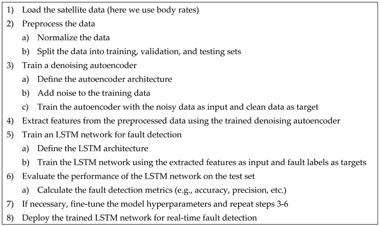
As articulated in Section 1, LSTM with denoising can be a suitable approach for satellite fault detection of reaction wheels due to its capability to model complex temporal-spatial patterns in noisy, high-dimensional flight data. Denoising LSTMs are designed to filter out noise and capture underlying patterns in the data, making them well-suited for identifying subtle changes in system behavior that could indicate potential faults. By processing the flight data with a denoising LSTM, it is possible to produce a denoised time series that is more suitable for fault detection. This denoised time series can then be analyzed using appropriate techniques to detect faults in the reaction wheels of the satellite, enabling timely maintenance and corrective action to be taken. In this research, we use the mentioned benefits of the LSTM for satellite reaction wheel fault detection via the steps explained in the pseudocode presented in Error! Reference source not found.. In the succeeding portion of this section, we shall delve into a detailed elucidation of the Long Short-Term Memory (LSTM) architecture, along with delineating the methodology for modeling time series data employing LSTM networks.

Table 1.
Pseudocode for LSTM-based Fault Detection.
 |
3.1. LSTM Network Architecture
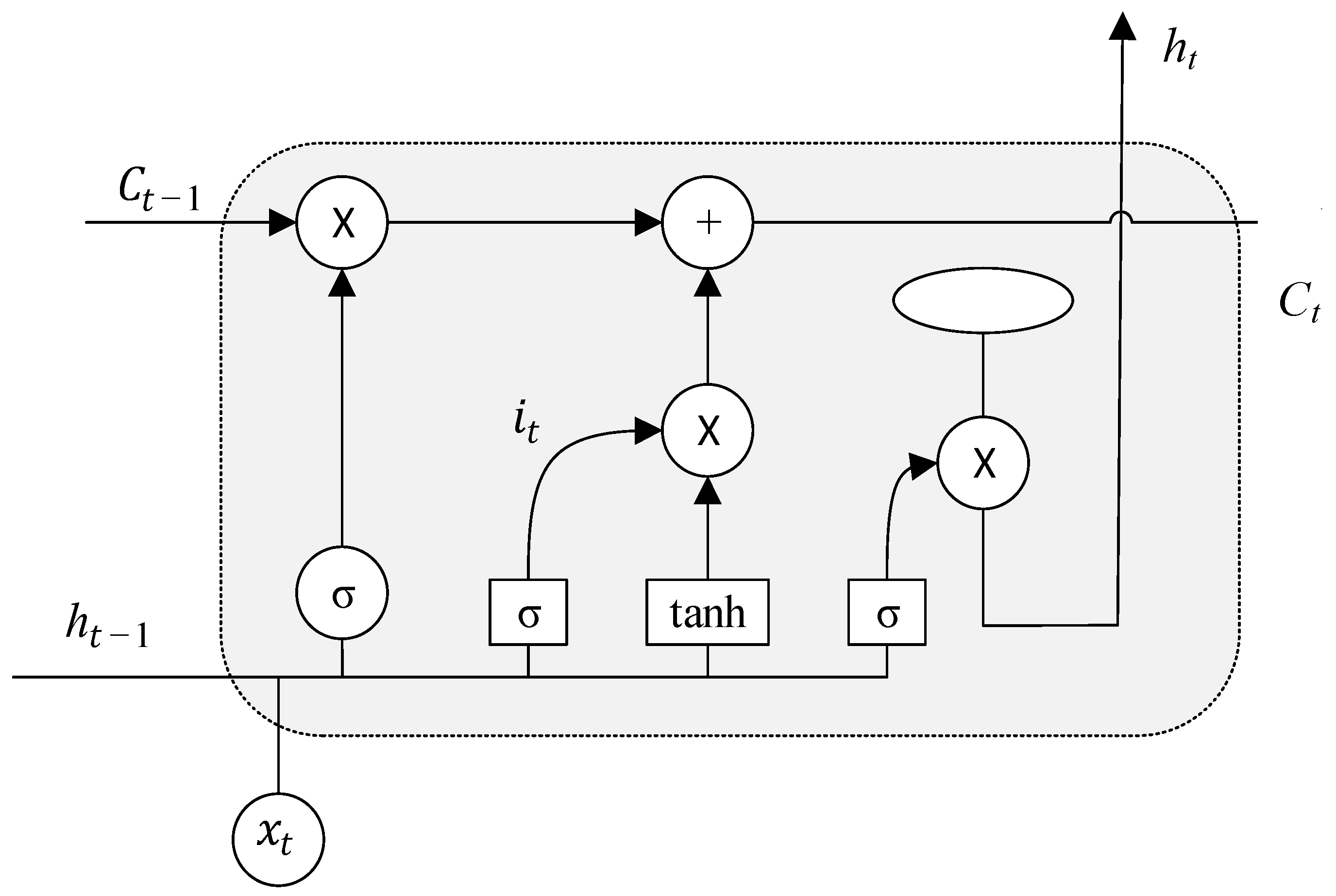
In using LSTM to identify faults in satellite reaction wheels, the first step involves deciding what information from the sensor data to discard from the cell state. This is accomplished using a "forget gate." This gate looks at the previous hidden state and current sensor input, assigning a value between 0 and 1 to each part of the cell state. A value of 1 means fully keep the information, while 0 means discard it completely. Next, we need to determine what new information will be stored in the cell state from the sensor readings. This involves two parts. Firstly, an "input layer" decides which values will be updated. Then, a new set of candidate data, representing potential faults, is created to be added to the cell state. Following this, these two parts come together to update the state. The previous state is adjusted by the forget gate value to disregard irrelevant information. Then, we add the new candidate data from the input gate, providing an updated state reflecting potential faults. Finally, we must decide what will be outputted to potentially signal a fault. This output is a filtered version based on our updated cell state. Firstly, a layer decides which parts of the cell state will be outputted. Then, we take the cell state, process it through a function (giving values between -1 and 1), and multiply it by the output of the previous layer. The parts we decided to output will be the final output, potentially signalling a fault in the satellite's reaction wheels. For a visual understanding of this LSTM layer process, please refer to Error! Reference source not found.. In this figure represents the states, is the input, each element in the cell state is represented by . and the forget gate is shown as f.
Figure 2.
LSTM layer schematic.
In our study, we use an LSTM network along with the SGDM (Stochastic Gradient Descent with Momentum) optimizer for finding faults in satellite reaction wheels (as presented in [33]). The SGDM optimizer is a bit different from the usual Stochastic Gradient Descent (SGD). While SGD changes the network settings like weights and biases little by little, going against the direction of the loss function's gradient, SGDM makes this process better by adding momentum.
3.2. Time Series Modeling Utilizing LSTM Networks
The objective of time series modeling is to construct a prognostic model that harnesses historical data to project future values. In the context of an LSTM-based fault detection methodology, discrepancies from these anticipated values could potentially indicate a fault. Within the purview of this study, we employ LSTM to predict the satellite's body rates. By leveraging the mean squared error between the predicted value and the simulated response, we discern the operational status of the system's reaction wheels, thereby identifying potential faults. In this work, we implement Long Short-Term Memory (LSTM) for time series prediction, as illustrated by the schematic in Error! Reference source not found.. The LSTM is designed to handle sequences, making it ideal for time series data.
In the LSTM architecture depicted, the state at each time step t is represented by , the input at each time step is , and each element in the cell state is represented by . The forget gate, crucial to LSTM operation, is represented by . The operations within an LSTM cell are summarized as follows:
- (1)
- The forget gate decides what information to discard from the cell state. This is determined by a sigmoid function, which outputs a value between 0 and 1 for each number in the cell state :
- (2)
- An input gate decides what new information to store in the cell state, and a tanh layer creates new candidate values , which could be added to the state:
The cell state is updated to the new state:
Finally, the output gate decides what part of the cell state is going to be outputted:
In the above eqiuations, represents the weight matrix for the forget gate in the LSTM cell. This matrix, when multiplied by the concatenated matrix of the previous hidden state and the current input, and added to the bias term (), is passed through the sigmoid function to decide which information should be kept (and which should be forgotten) in the cell state. Using these operations, the LSTM can predict the time series by learning these patterns over the input sequence x, and the output h represents the prediction for the next time step. Discrepancies between these predictions and actual sensor readings can signal potential faults in the satellite's reaction wheels.
Numerical Simulations and Results
4. Numerical Simulations Were Performed to Evaluate the Proposed LSTM-Based Fault Prediction Algorithm Algorithms. This Section Describes the Tests and Their Results
4.1. Test Setup
In this research, a Nano-satellite was employed as the representative spacecraft to showcase the techniques. The assumed inertia tensor of the satellite was denoted as .. The maximum speed of the wheels taken into account was 1200rad/s, and further details regarding the reaction wheels (RWs) can be found in Error! Reference source not found.. It should be emphasized that all RWs utilized in the experiments were presumed to be identical, with an initial wheel speed of 5rad/s. Error! Reference source not found. presents the constants employed for the objective function in this study. It is important to acknowledge that the occurrence of disturbances in RW torque may lead to extended settling durations. To establish a basis for comparison, this investigation defines a controller as settled on a given target once the norm of the pointing error falls below 0.001 rad. At this stage, the controller can commence the subsequent slew. One advantageous aspect of the torque allocation approach is their capability to optimize wheel speed patterns across multiple slews, thereby enhancing the spacecraft's agility and reducing the total time required to maneuver towards and stabilize at a series of designated pointing targets.
Table 2.
Specifications of the reaction wheels for the numerical simulations.
| Parameter | Value |
|---|---|
| Stall torque | 0.05 |
| Rotor inertia | 0.0008 |
| Torque constant | 0.103 |
| Back-EMF constant | 0.108 |
| Resonance number | 0.01 |
| Static friction | |
| Viscous friction | |
| Dynamic imbalance |
Table 3.
Objective function’s constants.
| Parameter | Value |
|---|---|
| 5 | |
| 0.01 | |
| 3 | |
| 0.05 | |
| 100 | |
| 100 | |
In order to assess the efficacy of the torque allocation approach, a comparison was made against the conventional pseudoinverse solution utilizing a Reaction Wheel Assembly (RWA) consisting of four wheels, with a configuration matrix defined in Equation (36). The evaluation comprised commanding a series of five sequential slews, each highlighting distinct wheel speed profiles. The initiation of each new slew was contingent upon the successful settling of the preceding one, adhering to the specified settling criteria outlined in the previous section.
4.1. Simulation Platform and Training Data Generation
To overcome the challenges of obtaining substantial fault data from real satellite missions, we implemented a simulation-based approach using MATLAB. This study focused on generating synthetic data from satellite reaction wheels under various fault conditions, including reaction wheel (RW) stiction, resonance, and viscous friction as discussed in Section 2.1. The synthetic data, with a time step of 20 ms, consisted of body rates of the satellite that are instrumental in detecting faults. The LSTM network served as the core of our fault detection system. By utilizing the simulated satellite sensor data, both with and without faults, the network learned to identify faults based on patterns in the body rates. This ability was then tested on the unseen dataset, providing a practical measure of its performance. At the end, we applied the Mean Squared Error (MSE) as a key metric to judge the quality of the LSTM predictions. In specific terms, we measured the MSE between the predicted and simulated body rate responses. If the MSE exceeded a predetermined threshold, the reaction wheel was classified as faulty.
4.2. Simulation Results
The satellite system delineated in Section 5.1 served as the experimental testbed for evaluating the performance of our LSTM-based fault detection system. Through simulations, the temporal variations in reaction wheel speed were plotted for both the pseudoinverse method and the null space method, with their corresponding satellite body rates under varying fault scenarios as well as in the absence of faults. Notably, for the LSTM network training, 1000 body rate values were utilized as input. The trained LSTM network was subsequently employed to predict the nominal response, which was then compared with the simulated responses, both faulty and healthy. The findings obtained from this process are systematically presented in the ensuing section.
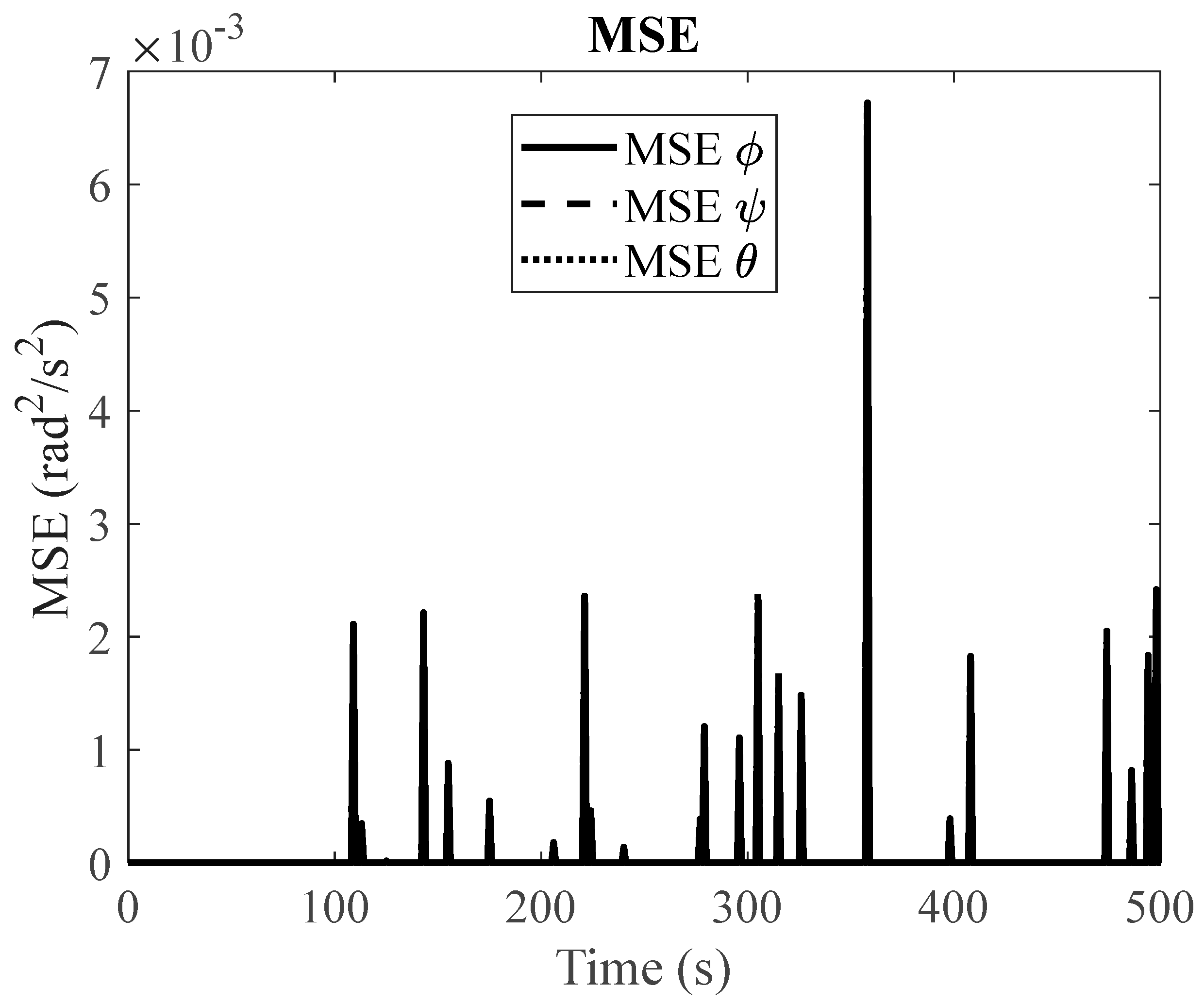
(1) Null Space Algorithm: To assess the effectiveness of our proposed algorithm, which employs an LSTM-based fault detection method with redundant reaction wheels, we begin by simulating the satellite system's slew performance under normal operating conditions. In addition, we conduct simulations for three distinct fault scenarios. When encountering faulty conditions, we generate graphical representations that display the Mean Squared Error (MSE) between the LSTM-based predicted response and the simulated faulty response. If the MSE exceeds the fault threshold, it serves as an indication of a potential fault within the system. Figure 3 and Figure 4 showcase the slew performance of the null space algorithm, illustrating the reaction wheel speeds and body rates, respectively. Figure 5, Figure 6, Figure 7, Figure 8, Figure 9, Figure 10, Figure 11, Figure 12 and Figure 13 present the simulation results for faulty reaction wheels, with three different faults, along with the LSTM prediction and their corresponding MSE.
(2) Pseudoinverse:
Figure 14.
Slew performance of the pseudoinverse algorithm (healthy RWs).
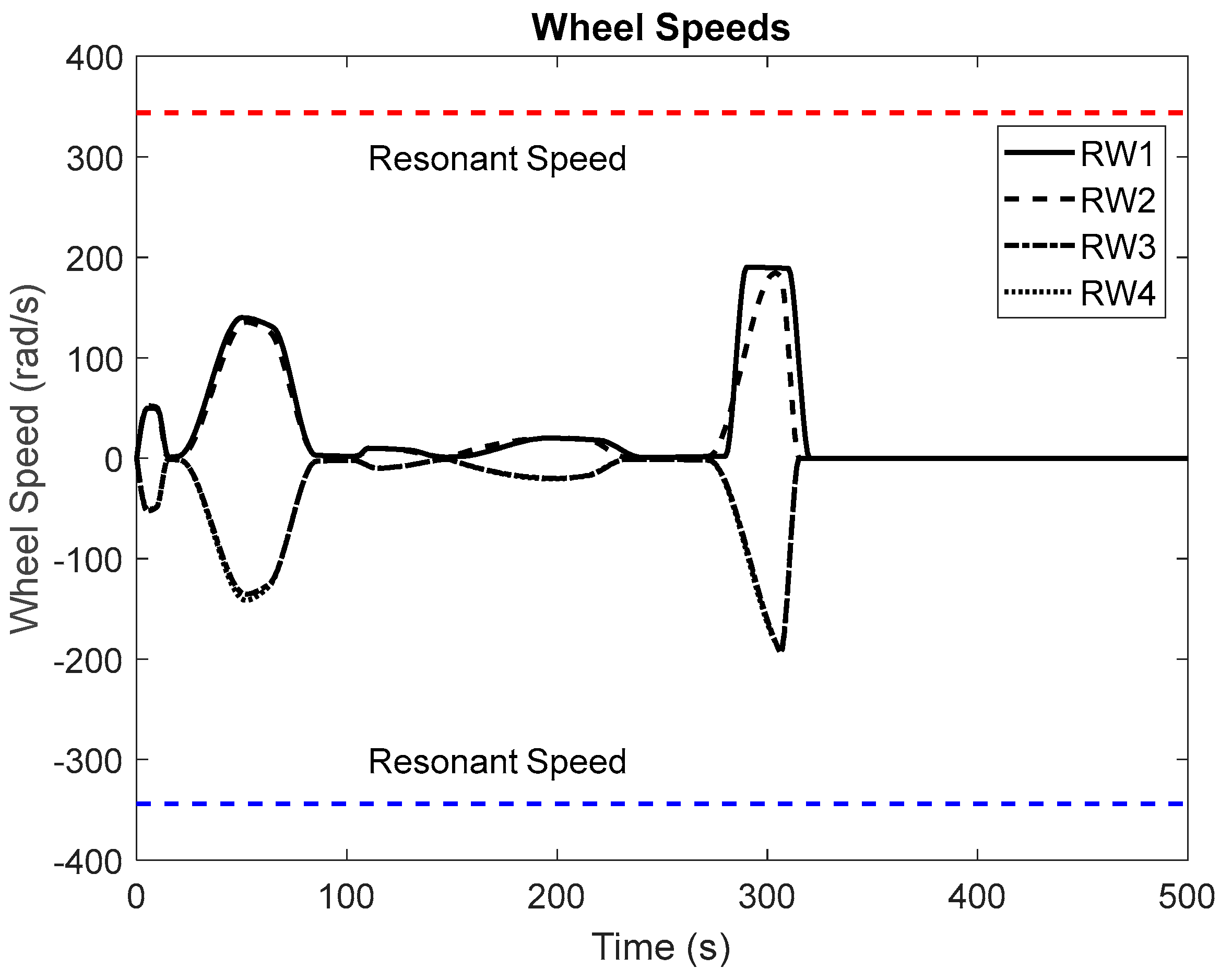
Figure 15.
MSE of body rates between LSTM predictions and faulty (stiction) simulations for pseudoinverse method.
Figure 15.
MSE of body rates between LSTM predictions and faulty (stiction) simulations for pseudoinverse method.
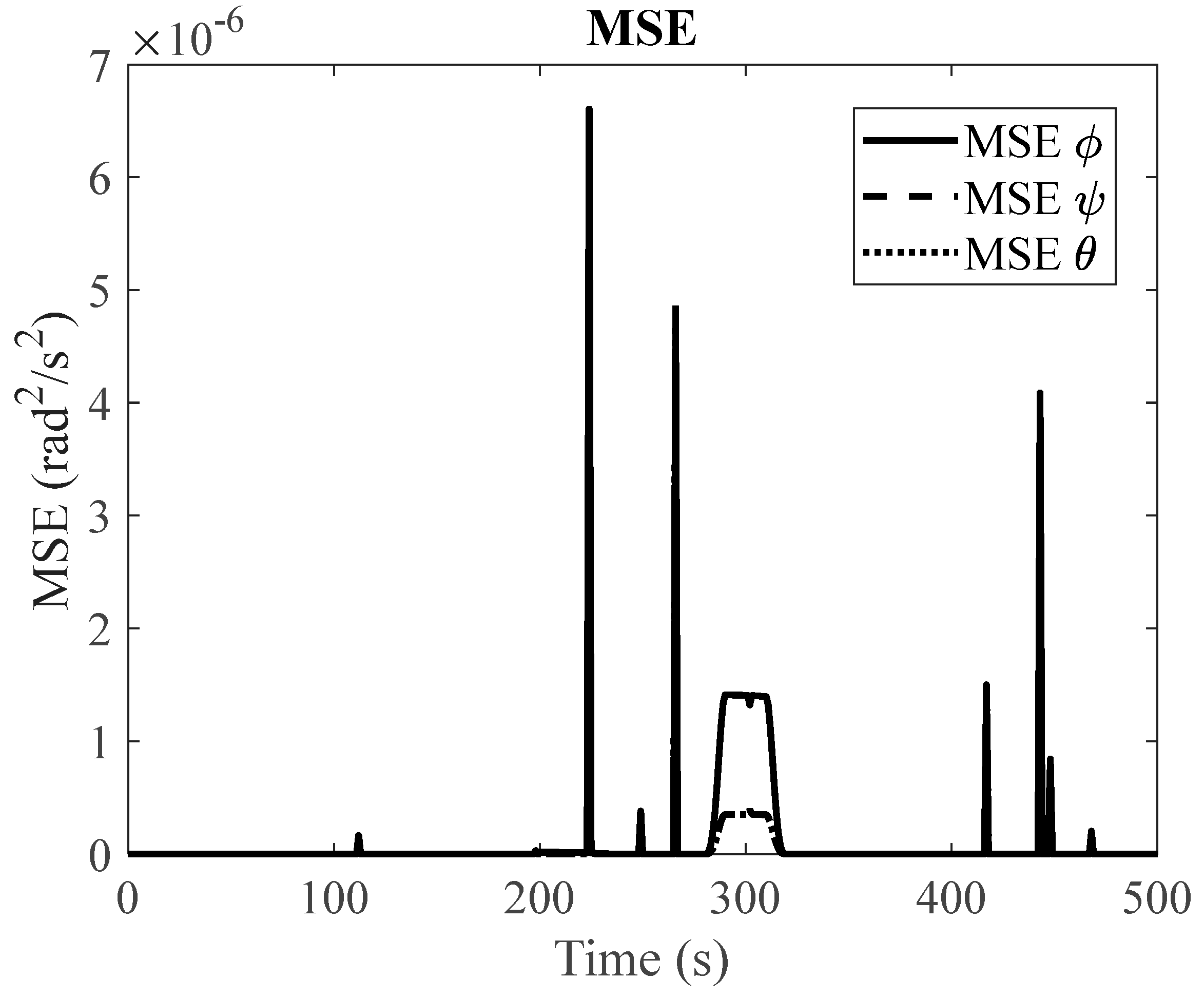
Figure 16.
MSE of body rates between LSTM predictions and faulty (Resonance) simulations for pseudoinverse method.
Figure 16.
MSE of body rates between LSTM predictions and faulty (Resonance) simulations for pseudoinverse method.
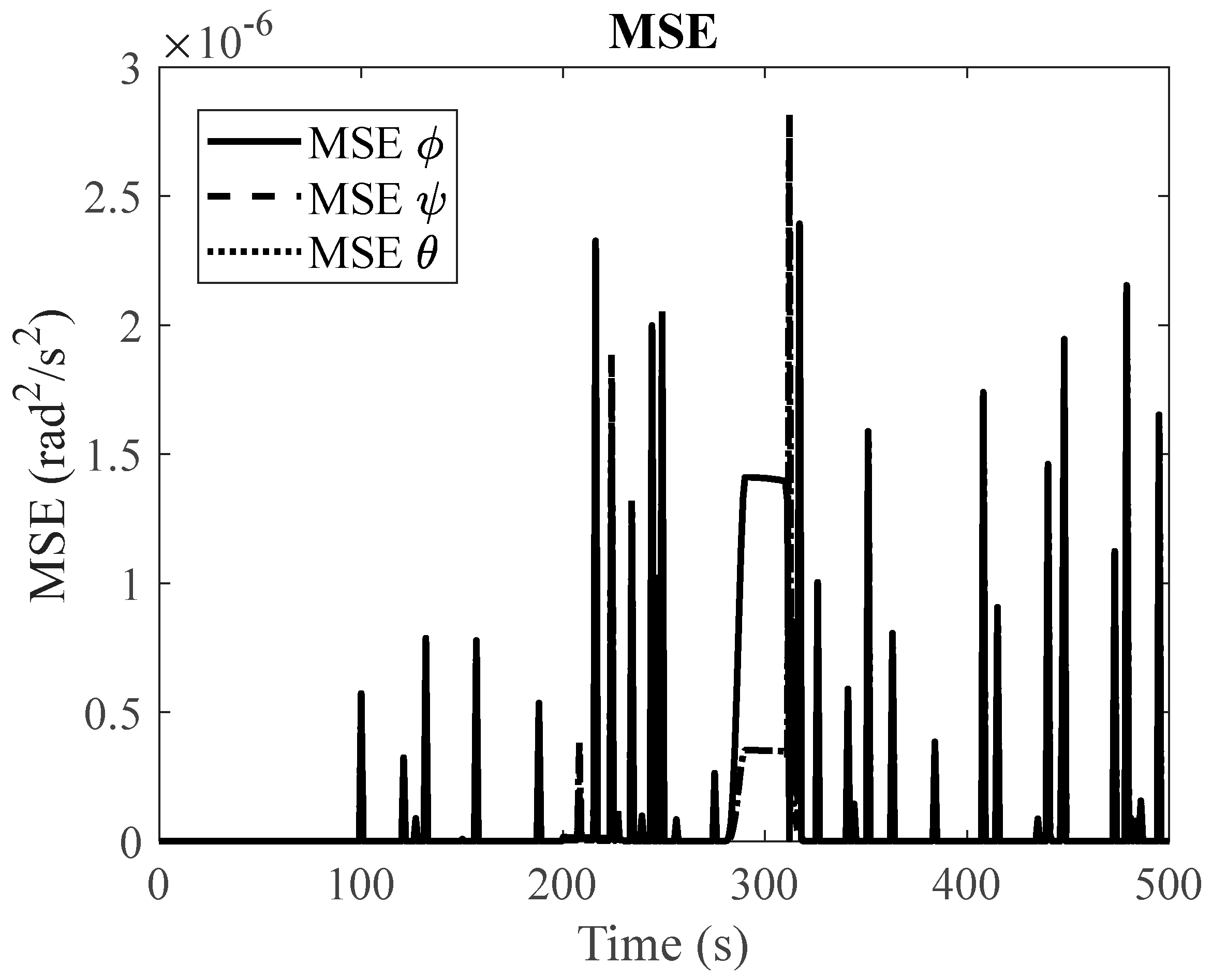
Figure 17.
MSE of body rates between LSTM predictions and faulty (viscous friction) simulations for pseudoinverse method.
Figure 17.
MSE of body rates between LSTM predictions and faulty (viscous friction) simulations for pseudoinverse method.
4.3. Discussion
To verify the efficacy of our fault detection methods, we utilize three key performance metrics, namely, the True Positive Rate (TPR), False Positive Rate (FPR), and overall Accuracy (Acc).
The True Positive Rate (TPR), also known as sensitivity or recall, measures the proportion of actual positives that are correctly identified. In our context, this refers to the percentage of actual faults that our system correctly detects.
The False Positive Rate (FPR), referred to as the fall-out, gauges the proportion of negative instances that are falsely flagged as positive. In our case, this indicates the percentage of non-fault events that our system incorrectly flags as faults.
The Accuracy (Acc) provides a holistic measure of the system's performance. It calculates the proportion of total predictions (both positive and negative) that are correct.
Furthermore, we evaluate the system's performance across varying fault intensities, specifically at 90%, 50%, and 30% of the maximum possible magnitude. These investigations, designed to emulate real-world variability, offer a thorough understanding of the system's response to diverse fault scenarios. The outcomes from these evaluations are encapsulated in Table 3. In most cases, we aim for a high TPR and a FPR. A high TPR is desirable as it indicates that the system is effectively identifying true positive instances, i.e., actual faults are accurately detected. A high TPR signifies a sensitive system capable of detecting most true faults. A low FPR is preferred as it suggests that the system rarely makes false alarms, i.e., it doesn't frequently misclassify non-fault situations as faults. A low FPR implies a precise system that can correctly disregard most non-fault instances. However, the balance between TPR and FPR is highly dependent on the application and the costs associated with false positives and false negatives. For some applications, it may be more important to have a higher TPR (even at the cost of increasing FPR) if the consequences of not detecting a true positive are severe. Conversely, in other applications, maintaining a low FPR may be more crucial if the repercussions of false alarms are high. Therefore, it's always important to adjust the system based on specific requirements and contexts.
5. Conclusion
In this study, we introduced a method based on LSTM deep learning to detect faults in satellite attitude control systems. Specifically, we focused on systems that rely on Reaction Wheels (RWs). Our approach effectively mitigated the negative impacts of torque disturbances related to velocity by integrating a torque allocation algorithm that utilizes redundant RWs. The results of our experiments demonstrated high accuracy in fault detection, improved system reliability, and enhanced performance. We validated the effectiveness of our proposed method in real-world scenarios, and we believe it can contribute to the existing range of fault detection and control techniques in satellite attitude control systems. To strengthen the robustness of our model in noisy data environments commonly encountered in space missions, we integrated denoising autoencoders within the LSTM architecture. This further improved its ability to function effectively. It is important to note that our model serves as a starting point and requires further refinements. For instance, its effectiveness under different operational circumstances and fault conditions needs extensive investigation. Nevertheless, this research highlights the potential of advanced machine learning algorithms such as LSTM in critical tasks within space technology. It signals an important era of intelligent and resilient space missions. Future research can focus on refining these methods and exploring their application in other subsystems of satellite technology. Through this paper, we aim to inspire further research in the integration of advanced machine learning techniques in space technology. This research has the potential to transform the way we conduct space missions by increasing reliability and efficiency.
References
- H. J. Park, S. H. J. Park, S. Kim, J. Lee, N. H. Kim, and J. H. Choi, “System-level prognostics approach for failure prediction of reaction wheel motor in satellites,” Advances in Space Research, vol. 71, no. 6, pp. 2691–2701, 2023. [CrossRef]
- S. Ahmed khan et al., “Active attitude control for microspacecraft; A survey and new embedded designs,” Advances in Space Research, vol. 69, no. 10, pp. 3741–3769, 2022. [CrossRef]
- G. Quinsac, B. G. Quinsac, B. Segret, C. Koppel, and B. Mosser, “Attitude control: A key factor during the design of low-thrust propulsion for CubeSats,” Acta Astronaut, vol. 176, pp. 40–51, 2020. [CrossRef]
- K. H. Lee, S. M. K. H. Lee, S. M. Lim, D. H. Cho, and H. D. Kim, “Development of Fault Detection and Identification Algorithm Using Deep learning for Nanosatellite Attitude Control System,” International Journal of Aeronautical and Space Sciences, vol. 21, no. 2, pp. 576–585, 2020. [CrossRef]
- T. Zhang and P. Ferguson, “Optimal Reaction Wheel Disturbance Avoidance via Torque Allocation Algorithms,” Journal of Guidance, Control, and Dynamics, vol. 46, no. 1, pp. 152–160, 2023. [CrossRef]
- S. Ahmed khan, Y. S. Ahmed khan, Y. Shiyou, A. Ali, M. Tahir, S. Fahad, and S. Rao, “CubeSats detumbling using only embedded asymmetric magnetorquers,” Advances in Space Research, vol. 71, no. 5, pp. 2140–2154, 2023. [CrossRef]
- M. Alger and A. de Ruiter, “Magnetic spacecraft attitude stabilization with two torquers,” Acta Astronaut, vol. 192, pp. 157–167, 2022. [CrossRef]
- M. S. Islam and A. Rahimi, “A three-stage data-driven approach for determining reaction wheels’ remaining useful life using long short-term memory,” Electronics (Switzerland), vol. 10, no. 19, p. 2432, 2021. [CrossRef]
- T. Nagata, T. T. Nagata, T. Nonomura, K. Nakai, K. Yamada, Y. Saito, and S. Ono, “Data-Driven Sparse Sensor Selection Based on A-Optimal Design of Experiment with ADMM,” IEEE Sens J, vol. 21, no. 13, pp. 15248–15257, 2021. [CrossRef]
- W. Sun et al., “A simple and effective spectral-spatial method for mapping large-scale coastal wetlands using China ZY1-02D satellite hyperspectral images,” International Journal of Applied Earth Observation and Geoinformation, vol. 104, p. 102572, 2021. [CrossRef]
- H. Yoon, “Maximum Reaction-Wheel Array Torque/Momentum Envelopes for General Configurations,” Journal of Guidance, Control, and Dynamics, vol. 44, no. 6, pp. 1219–1223, 2021. [CrossRef]
- D. Aicardi, P. D. Aicardi, P. Musé, and R. Alonso-Suárez, “A comparison of satellite cloud motion vectors techniques to forecast intra-day hourly solar global horizontal irradiation,” Solar Energy, vol. 233, pp. 46–60, 2022. [CrossRef]
- Q. Hu, X. Q. Hu, X. Shao, and L. Guo, Intelligent Autonomous Control of Spacecraft with Multiple Constraints. Springer Nature, 2023.
- H. Abbasi Nozari, P. H. Abbasi Nozari, P. Castaldi, S. J. Sadati Rostami, and S. Simani, “Hybrid robust fault detection and isolation of satellite reaction wheel actuators,” Journal of Control and Decision, pp. 1–15, 2022.
- P. Castaldi, H. A. P. Castaldi, H. A. Nozari, J. Sadati-Rostami, H. D. Banadaki, and S. Simani, “Intelligent hybrid robust fault detection and isolation of reaction wheels in satellite attitude control system,” in 2022 IEEE 9th International Workshop on Metrology for AeroSpace (MetroAeroSpace), IEEE, 2022, pp. 441–446.
- A.-E. R. Abd-Elhay, W. A. A.-E. R. Abd-Elhay, W. A. Murtada, and M. I. Youssef, “A Reliable Deep Learning Approach for Time-Varying Faults Identification: Spacecraft Reaction Wheel Case Study,” IEEE Access, vol. 10, pp. 75495–75512, 2022.
- Z. Chen, “Satellite Reaction Wheel Fault Detection Based on Adaptive Threshold Observer,” in 2021 Global Reliability and Prognostics and Health Management (PHM-Nanjing), IEEE, 2021, pp. 1–6.
- Rahimi, K. D. Kumar, and H. Alighanbari, “Fault estimation of satellite reaction wheels using covariance based adaptive unscented Kalman filter,” Acta Astronaut, vol. 134, pp. 159–169, 2017.
- S. K. Ibrahim, A. S. K. Ibrahim, A. Ahmed, M. A. E. Zeidan, and I. E. Ziedan, “Machine learning techniques for satellite fault diagnosis,” Ain Shams Engineering Journal, vol. 11, no. 1, pp. 45–56, 2020.
- Choudhary, T. Mian, and S. Fatima, “Convolutional neural network based bearing fault diagnosis of rotating machine using thermal images,” Measurement, vol. 176, p. 109196, 2021.
- M. S. Islam and A. Rahimi, “Fault prognosis of satellite reaction wheels using a two-step LSTM network,” in 2021 IEEE International Conference on Prognostics and Health Management (ICPHM), IEEE, 2021, pp. 1–7.
- M. Jalayer, C. M. Jalayer, C. Orsenigo, and C. Vercellis, “Fault detection and diagnosis for rotating machinery: A model based on convolutional LSTM, Fast Fourier and continuous wavelet transforms,” Comput Ind, vol. 125, p. 103378, 2021.
- S. Belagoune, N. S. Belagoune, N. Bali, A. Bakdi, B. Baadji, and K. Atif, “Deep learning through LSTM classification and regression for transmission line fault detection, diagnosis and location in large-scale multi-machine power systems,” Measurement, vol. 177, p. 109330, 2021.
- S. S. Afshari, C. S. S. Afshari, C. Zhao, X. Zhuang, and X. Liang, “Deep learning-based methods in structural reliability analysis: a review,” Meas Sci Technol, 2023.
- K. J. Reckdahl, “Wheel speed control system for spacecraft with rejection of null space wheel momentum.”. Google Patents , Oct. 31, 2000.
- S. Ratan and X. Li, “Optimal speed management for reaction wheel control system and method.”. Google Patents , Apr. 03, 2007.
- Kron, A. St-Amour, and J. de Lafontaine, “Four reaction wheels management: Algorithms trade-off and tuning drivers for the PROBA-3 mission,” IFAC Proceedings Volumes, vol. 47, no. 3, pp. 9685–9690, 2014.
- R. Rigger, “On stiction, limit and constraint avoidance for reaction wheel control,” in SpaceOps 2010 Conference Delivering on the Dream Hosted by NASA Marshall Space Flight Center and Organized by AIAA, 2010, p. 1931.
- F. A. Leve, B. J. F. A. Leve, B. J. Hamilton, M. A. Peck, F. A. Leve, B. J. Hamilton, and M. A. Peck, “Momentum-Control System Array Architectures,” Spacecraft Momentum Control Systems, pp. 133–155, 2015.
- Y. Wang and S. Xu, “Gravity gradient torque of spacecraft orbiting asteroids,” Aircraft Engineering and Aerospace Technology, vol. 85, no. 1, pp. 72–81, 2013.
- R. A. Masterson, “Development and validation of empirical and analytical reaction wheel disturbance models.” Massachusetts Institute of Technology, 1999.
- Dresden, “The fourteenth western meeting of the American Mathematical Society.” 1920.
- M. Turkoglu, D. M. Turkoglu, D. Hanbay, and A. Sengur, “Multi-model LSTM-based convolutional neural networks for detection of apple diseases and pests,” J Ambient Intell Humaniz Comput, pp. 1–11, 2019.
Figure 3.
Slew performance of the null space algorithm (healthy RWs).
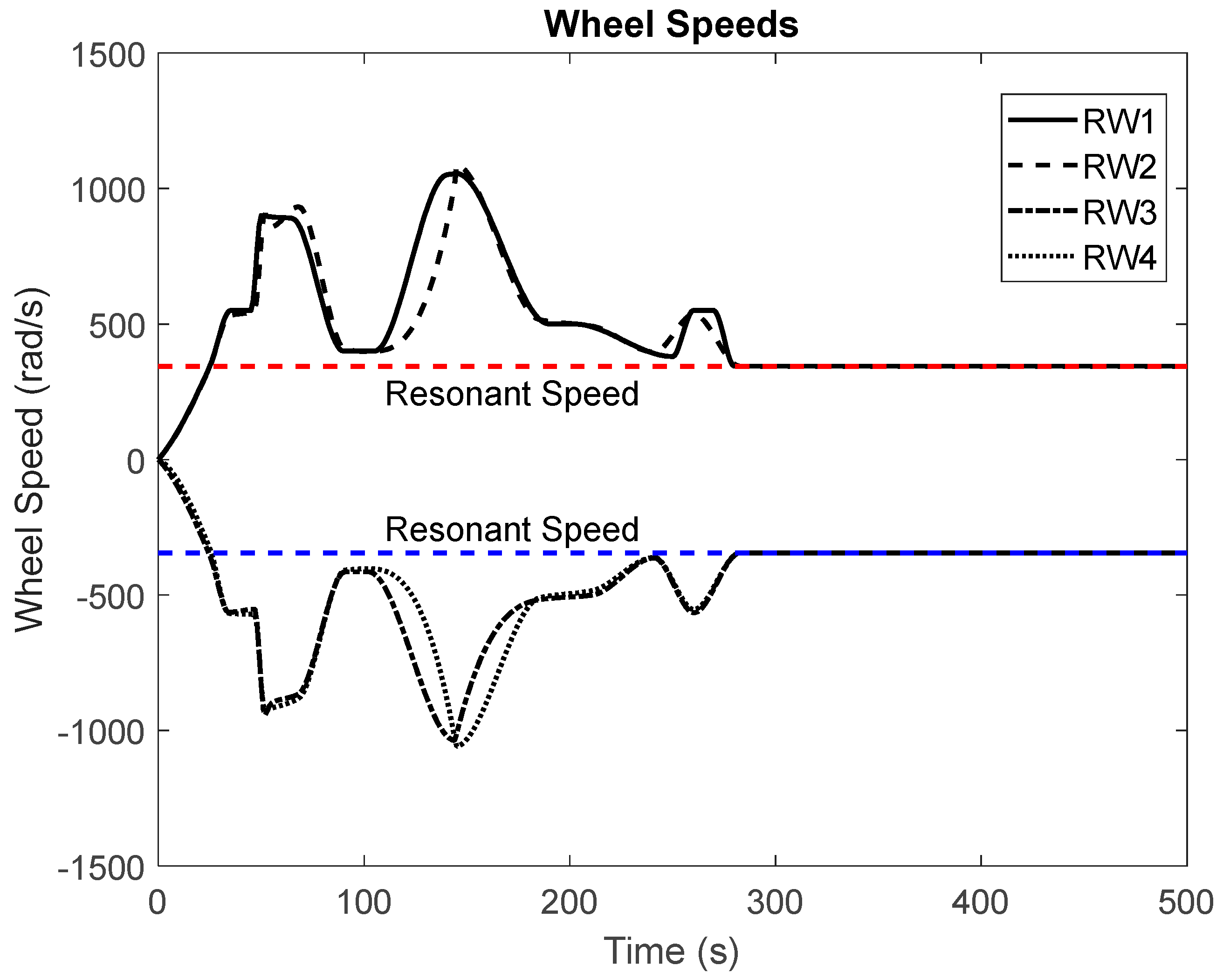
Figure 4.
Body rates of a healthy system (null space algorithm).
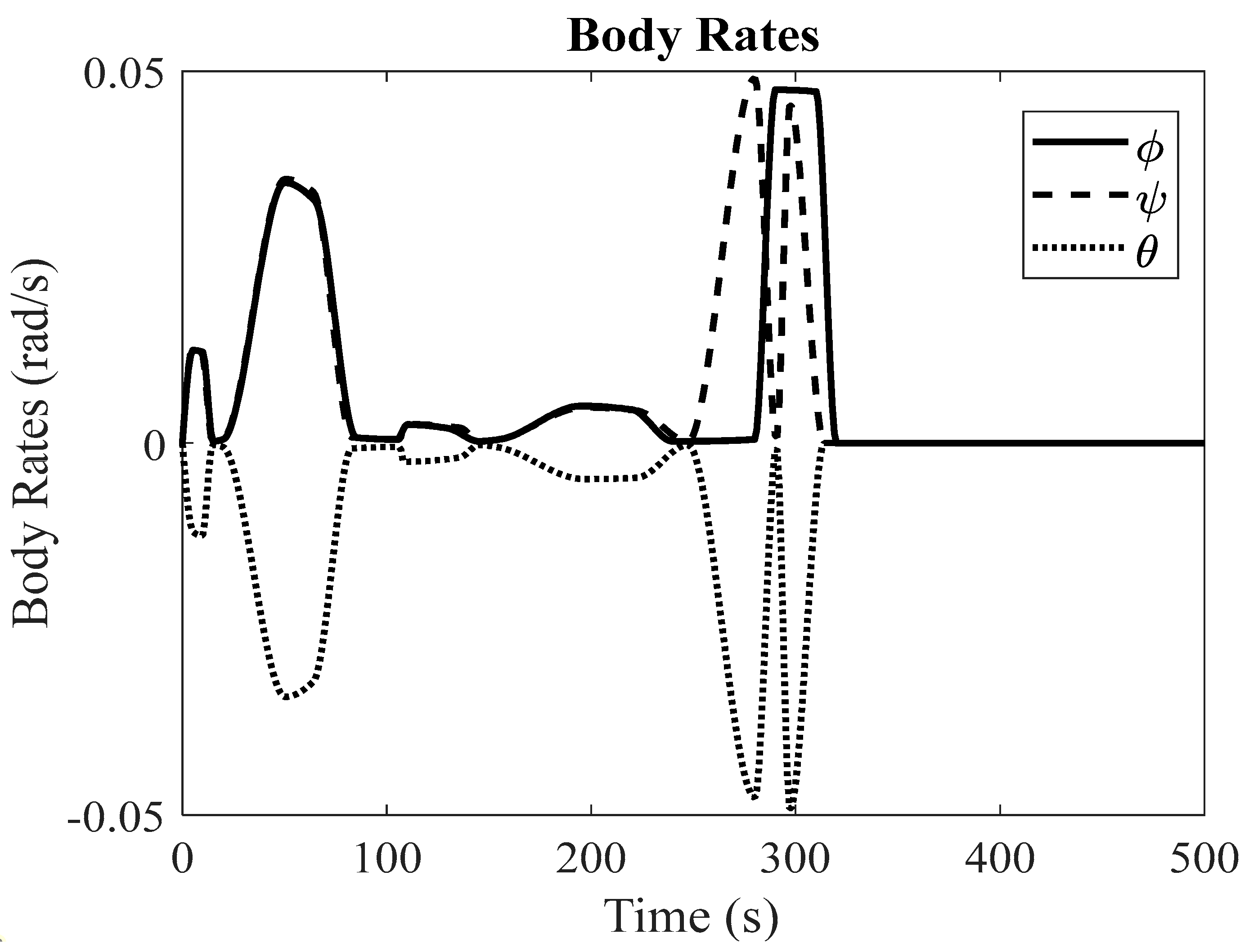
Figure 5.
Slew performance of the null space algorithm (Faulty RW: RW2 resonance at t=100).

Figure 6.
Body rates of faulty condition and LSTM prediction of healthy body rates ().
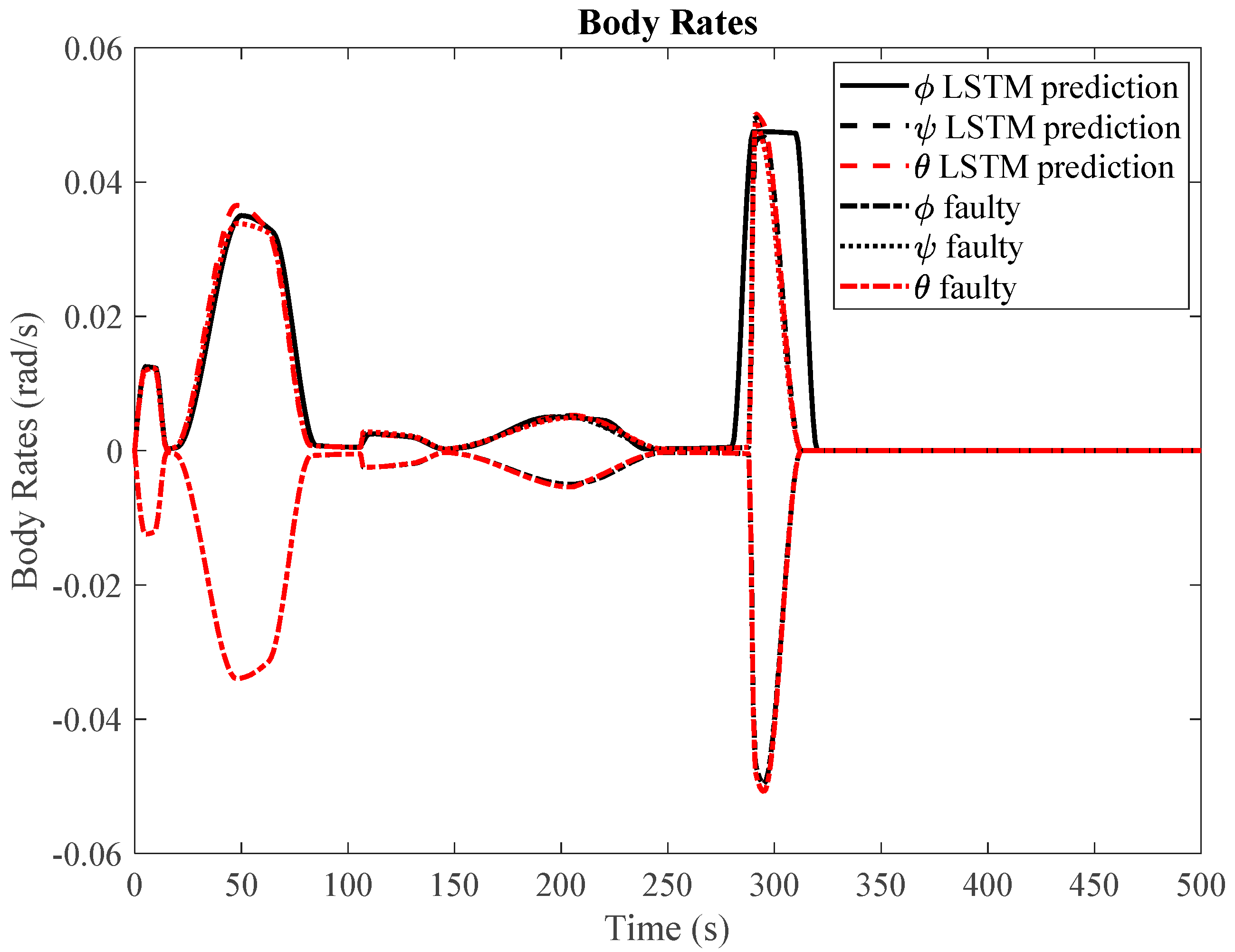
Figure 7.
Mean Squared Error (MSE) of body rates between LSTM predictions and faulty simulations (RW2 resonance at t=100).
Figure 7.
Mean Squared Error (MSE) of body rates between LSTM predictions and faulty simulations (RW2 resonance at t=100).
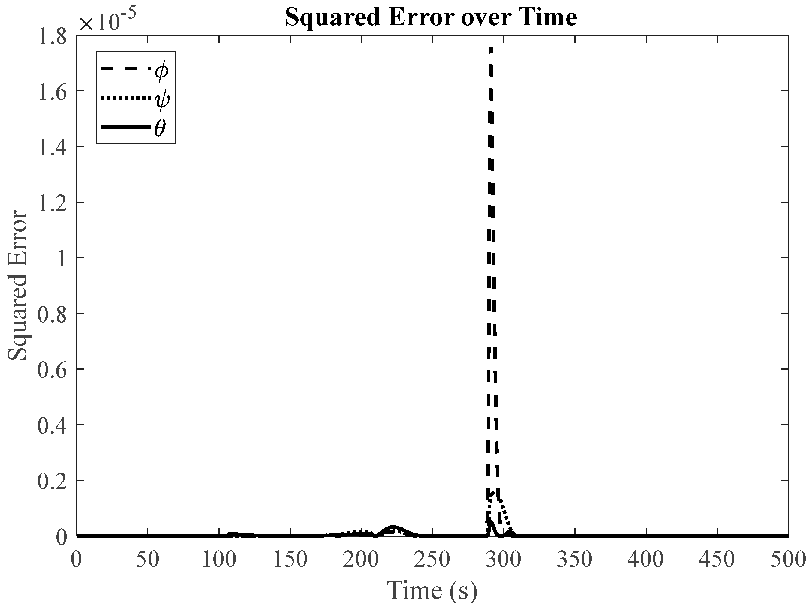
Figure 8.
RW2 resonance at t=100 RW2 stiction Cstic= 0.04.
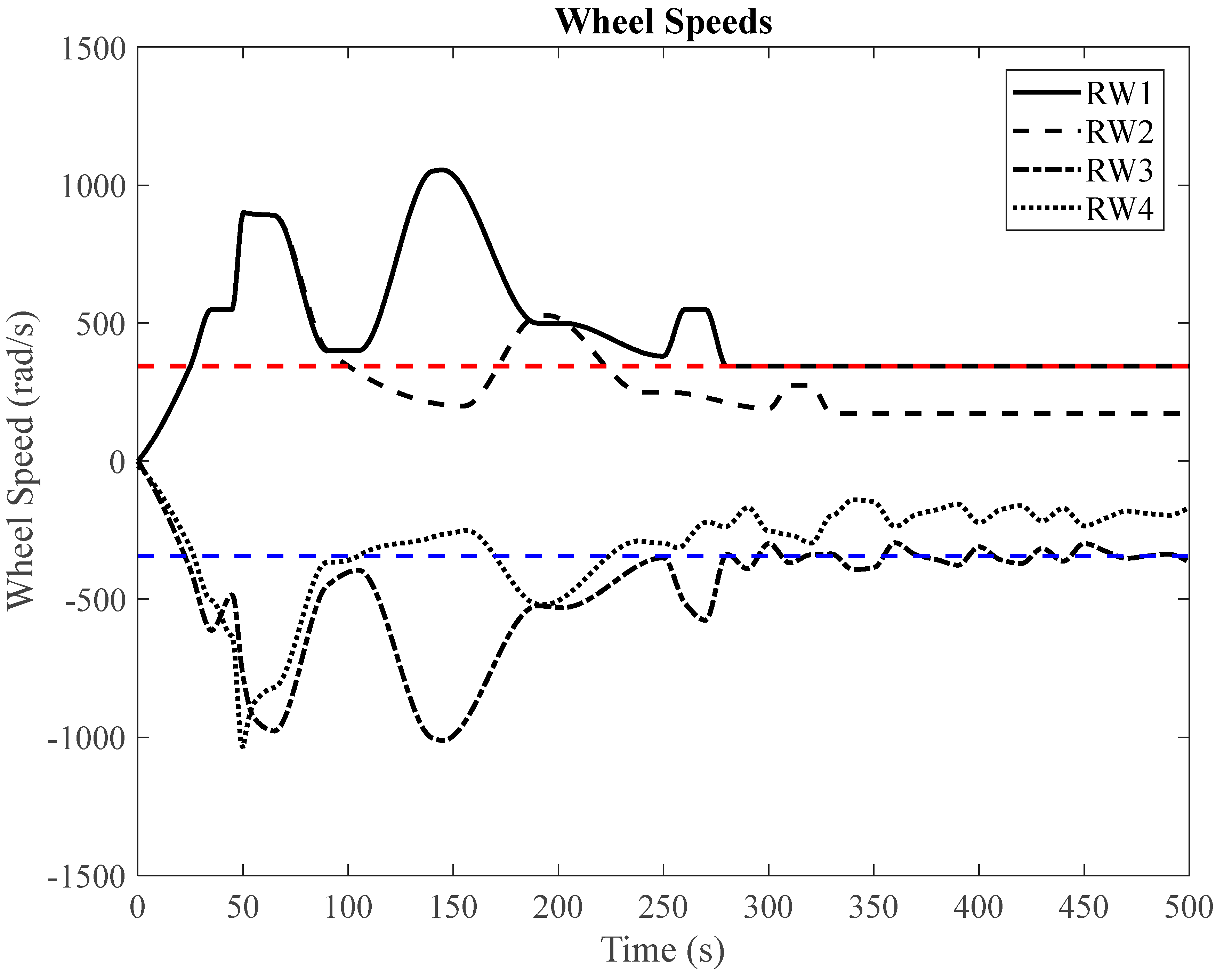
Figure 9.
Body rates of faulty condition and LSTM prediction of healthy body rates (RW2 stiction Cstic= 0.04).
Figure 9.
Body rates of faulty condition and LSTM prediction of healthy body rates (RW2 stiction Cstic= 0.04).
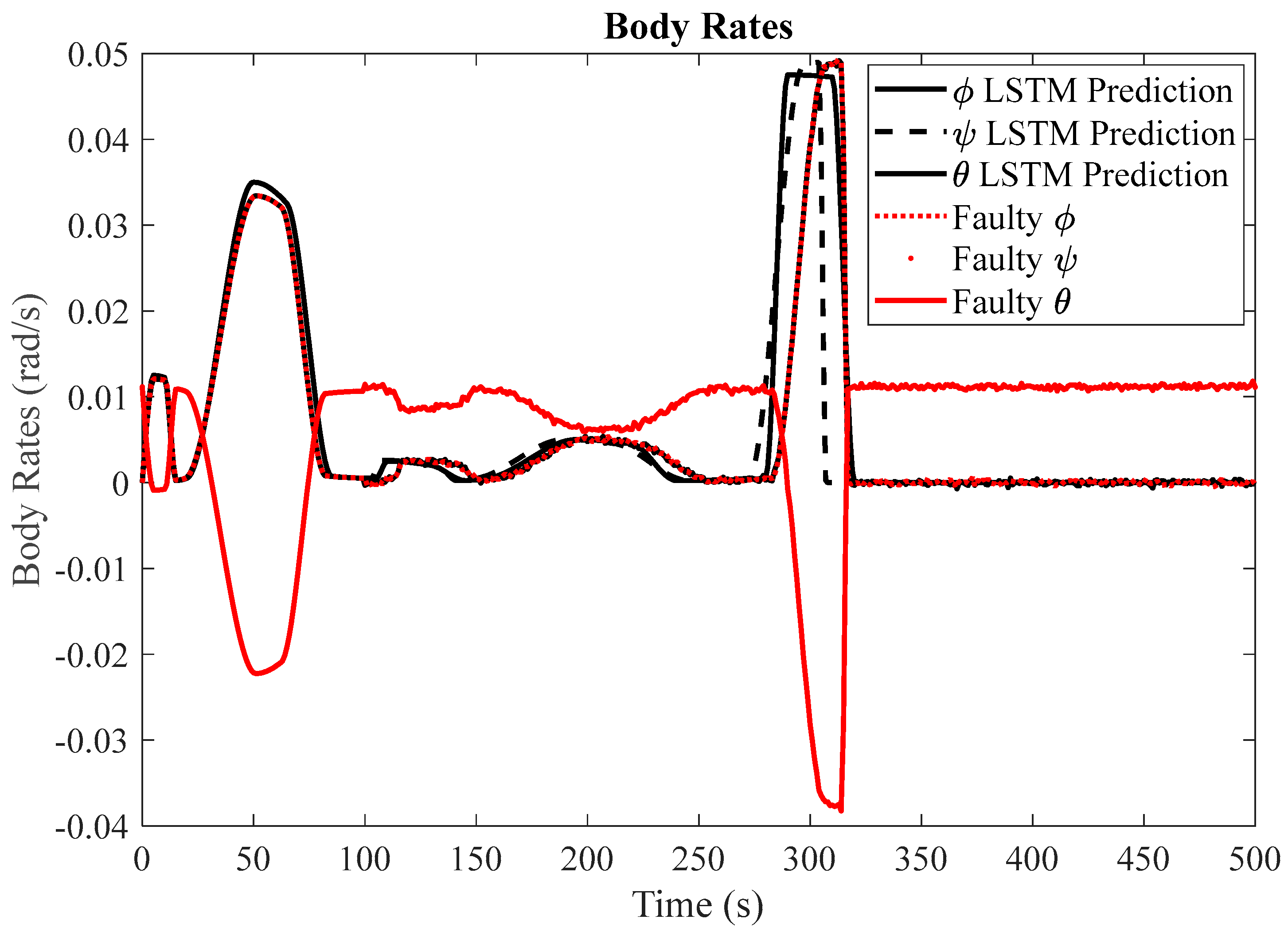
Figure 10.
Mean Squared Error (MSE) of body rates between LSTM predictions and faulty simulations (RW2 stiction Cstic= 0.04).
Figure 10.
Mean Squared Error (MSE) of body rates between LSTM predictions and faulty simulations (RW2 stiction Cstic= 0.04).
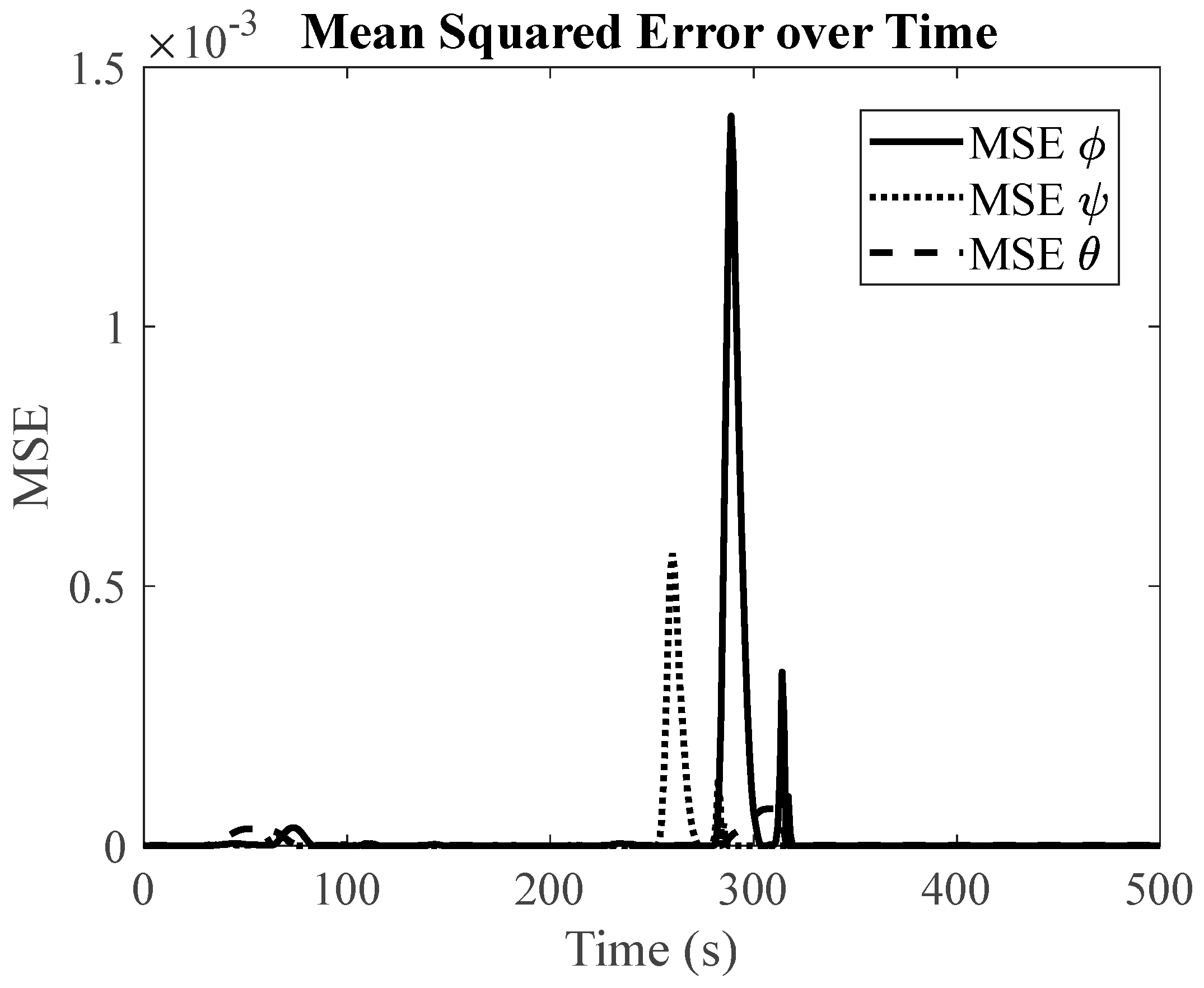
Figure 11.
Slew performance of the null space algorithm (RW2 viscous friction).
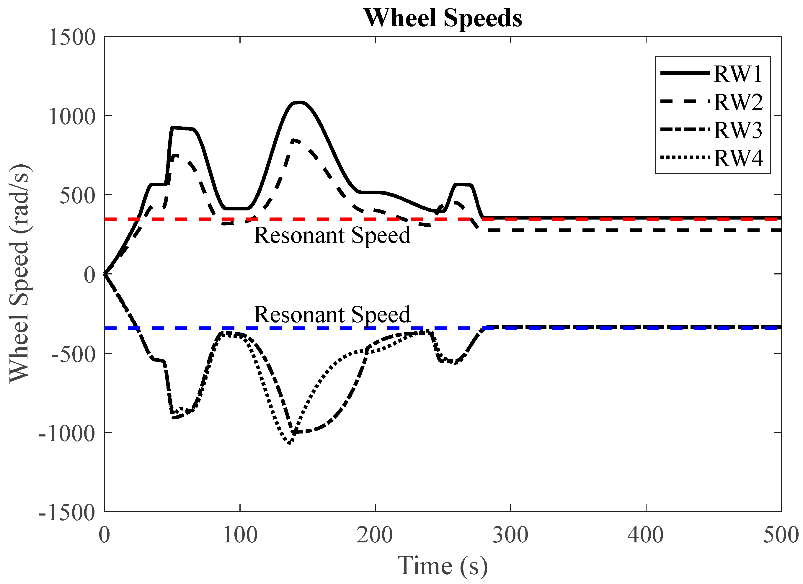
Figure 12.
Body rates of faulty condition and LSTM prediction of healthy body rates (RW2 stiction Cstic= 0.04).
Figure 12.
Body rates of faulty condition and LSTM prediction of healthy body rates (RW2 stiction Cstic= 0.04).
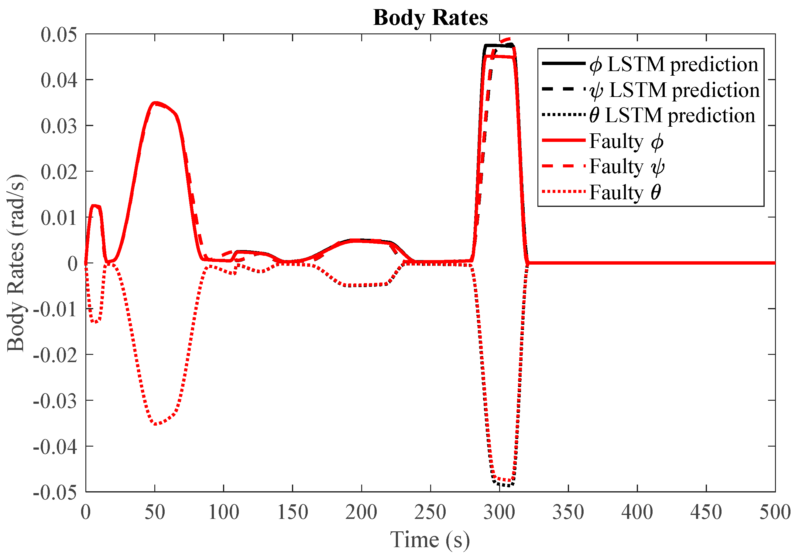
Figure 13.
Mean Squared Error (MSE) of body rates between LSTM predictions and faulty simulations.
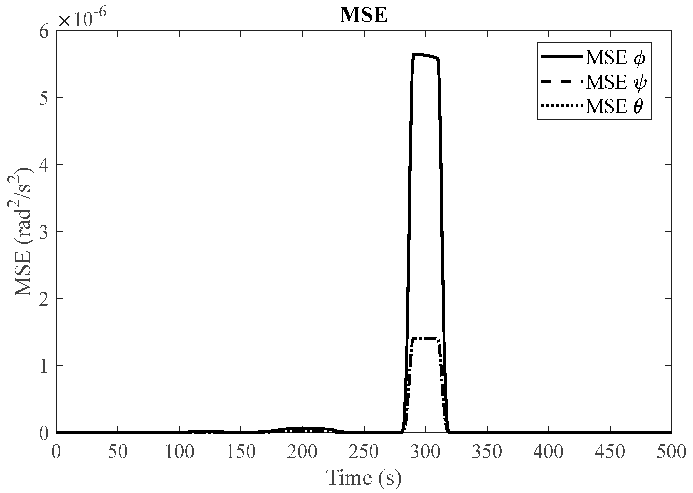
Table 4.
fault detection results simulated reaction wheel fault.
| Fault Amplitude | Approach | Acc | TPR | FPR |
|---|---|---|---|---|
| 80% | LSTM | 0.0926 | 0.0891 | 0.0402 |
| LSTM-DAE | 0.8950 | 0.0885 | 0.0325 | |
| LSTM-DAE (RRW) | 0.0956 | 0.0879 | 0.0057 | |
| 40% | LSTM | 0.0853 | 0.0725 | 0.0396 |
| LSTM-DAE | 0.0866 | 0.0676 | 0.0359 | |
| LSTM-DAE (RRW) | 0.0912 | 0.0704 | 0.0055 | |
| 20% | LSTM | 0.0722 | 0.0622 | 0.0391 |
| LSTM-DAE | 0.0785 | 0.0663 | 0.0300 | |
| LSTM-DAE (RRW) | 0.0896 | 0.0698 | 0.0031 |
Disclaimer/Publisher’s Note: The statements, opinions and data contained in all publications are solely those of the individual author(s) and contributor(s) and not of MDPI and/or the editor(s). MDPI and/or the editor(s) disclaim responsibility for any injury to people or property resulting from any ideas, methods, instructions or products referred to in the content. |
© 2024 by the authors. Licensee MDPI, Basel, Switzerland. This article is an open access article distributed under the terms and conditions of the Creative Commons Attribution (CC BY) license (http://creativecommons.org/licenses/by/4.0/).
Copyright: This open access article is published under a Creative Commons CC BY 4.0 license, which permit the free download, distribution, and reuse, provided that the author and preprint are cited in any reuse.


