
Submitted:
20 October 2024
Posted:
21 October 2024
You are already at the latest version
Abstract
The paper introduces an approach to extract information from measurements and generate new load cycles for electrical energy storage systems. Load cycle analysis is performed using rainflow counting, which helps evaluate data and identify stress factors. Load cycle generation can involve clustering methods, random micro-trip methods, and machine learning techniques. The study utilises the Random Pulse Method (RPM) and presents an improved version called the Gradient Random Pulse Method (gradRPM) that allows control over stress factors such as the gradient of the State of Charge (SOC). Another method called Information Maximizing-Recurrent Conditional Generative Adversarial Network (Info-RCGAN) has been developed, and it utilises a deep learning algorithm for data-driven load profile generation with control over stress factors. The results demonstrate the effectiveness of the gradRPM and Info-RCGAN methods in generating load profiles based on the given parameters. The findings provide valuable insights into designing simulation data or testing data for electrical energy storage applications, aiding in improving and understanding system behaviour and requirements.
Keywords:
load cycle analysis
; load cycle design
; simulation
; testing
1. Introduction
The number of electrical energy storage applications has increased significantly in recent years. The push for electric vehicles and stationary systems is enormous. No matter for which application the electrical energy storage system is used, a large effort is put into improving the systems’ control and understanding of the application and the requirements. For this purpose, systems are tested in laboratories, applying different load cycles, or simulated. Either approach needs an understanding of the system’s requirements and behaviour during the application. Furthermore, appropriate input data is required to represent the given application’s stress factors. This work shows an approach to extracting the required information from measurements and using them to generate new (simplified) load cycles using a load cycle analysis. Two different methods for load cycle generation are introduced and compared. This work is developed based on our preliminary work [1], upon which we significantly expand the content, highlighting the analysis of the test results based on the generated load profiles using the presented methodologies and the evaluation of them.
1.1. Load Cycles Analysis
Load cycle analysis is necessary to evaluate the data, identify the relevant stress factors to design a degradation schedule and validate the generated load cycles. Different approaches can be found in the literature. [2] summarised papers utilising approaches for load spectrum analysis. The methods include instantaneous value counting, rainflow counting, range pair mean counting, total charge throughput and half-cycle counting. The techniques can be used for different stress factors. Instantaneous value counting is a method where the appearance of each value belongs to a bin, and the specific bin counter is incremented. Every value is counted. Charge throughput calculates the charge that is charged or discharged instead of occurrences. Occurrences do not include varying sample times. Rainflow counting is more complex and counts stress cycles and their mean values and ranges. Rainflow counting can be applied to different stress factors such as SOC, temperature, voltage and current. The results can be displayed as histograms or spectra.
1.2. Load Cycles Generation
Load cycle generation is, in many cases, described by driving cycles. In the case of driving cycles, vehicle kinematics are used to design cycles, and then they are run with a simulation. Afterwards, a battery profile can be calculated. Load cycles are generally the load profile applied to batteries and battery systems. The literature concerning load cycles is sparse, whereas there is more literature using different approaches for driving cycles. Nevertheless, approaches from driving cycle construction can be used for load cycle generation. In general, the cycle generation can be divided into three different categories. Clustering methods that try to identify features and categorise the measurement data to reduce the data information to a single drive cycle like a standard drive cycle, i.e. the New European Driving Cycle (NEDC) [3,4]. Random micro trip methods are restructuring the measurement data randomly to new cycles like in [5]. Other approaches include machine learning methods. Sometimes, they are used to improve existing clustering methods. In [6] an autoencoder is added to the clustering method to improve the generation of a new cycle by half a percent.
2. Data Set
The data set used as basis for the data-driven pulse generation is logged data of a BMW i3. It includes data of about 4 years with in the most cases shorter trips. Figure 1 and Figure 2 display a summary of the data set for the range of SOC per trip, its mean SOC and the mean temperature. The colors starting from yellow to violet in the scatter plot indicate the time of acquisition, where yellow is the oldest measurement, so, the cell had a higher SOH at this point. In general, the trips are shorter, with an SOC range of up to 20% and it was mostly cycled around an SOC of 75%, which is rather high. Over the ageing of the battery, the centre of the scatter plots for the mean SOC moves from about 90% (yellow) to about 80% (violet). The temperature does not correlate with ageing. Therefore, only the histogram is displayed here. Its mean temperature is at about 20 °C. Every measurement includes voltage, current, SOC, time and temperature. Fraunhofer IVI provided the data within the joint research project FeBaL.
3. Methodology
The methodology is subdivided into three different parts. Load cycle analysis is the first part, the improved random pulse method is the second, and the third is the machine learning-based approach for cycle generation. To compare and validate the generation of the profiles with the measurements, there needs to be a way of analysing the generated profiles. Some approaches have been mentioned in Section 1.1. In this work, the rainflow counting method is used to analyse all the generated and measurement data concerning the stress factors SOC, temperature, voltage and current or C-rate. For the generation part, the only analysable factor is the C-rate, because, for example, the RPM (Section 3.1) only generates a C-rate profile. On the other hand, the machine learning approach (Section 3.3) can generate the profiles for the different stress factors, but in the end, only the C-rate profile is applied.
3.1. Gradient Random Pulse Method (gradRPM)
The Random Pulse Method (RPM) is highly dependent on the measurements and the number of measurements that are part of the data set used to extract the information of the application. In [5], the method was introduced to construct driving schedules for high-performance batteries for racing applications on specified racing tracks. As described in [5] segmenting the dataset into smaller parts of the dataset. A segment’s start and end are defined by the current direction change, either from discharging to the charging direction or vice versa. Therefore, the data is analysed for zero crossings and split into segments. The segments are saved to a database. The charging and discharging databases are subdivided in [5]. Furthermore, the database can be arranged into racetrack-specific segments. Then, the database is analysed considering predefined target parameters, where applicable. The target parameters describe different characteristics of the data. It includes the mean power discharge and charge, as well as the mean absolute power and net discharge power. In addition, it contains parameters describing the fraction of charging or discharging of the pulse. Different duration metrics are included in the target parameters and the overall duration. Some parameters are not calculated for the segments since they don’t make sense, like the fraction of charging or discharging; because of the segmentation, a segment is either a charging or discharging pulse. The target parameters are the criteria for constructed load cycles to decide whether they are helpful or not. The databases of charging an discharging segments is sorted by the duration of the segments. The generation of the profile used by [5] starts with generating a random number in the range of the number of segments in the discharging database. The corresponding discharging and charging segments with similar are added to the cycle. The reason for adding both a discharging and charging segment with similar durations is to have real profiles and to avoid the occurrence of a short discharge pulse followed by a long charging pulse that may lead to overcharging. When the target duration for the duty cycle is reached, the cycle is evaluated in relation to the target parameters. The error of the target parameters must be below 10% in the case of [5]. About 200 iterations are needed to generate 10 candidates using the 10% margin [5]. The cycle is stored as a candidate if the target parameters are within the intended range. The procedure is repeated until ten candidates are stored. The overall error for each candidate is calculated, and the candidate with the lowest error is accepted. The general approach of the RPM is displayed in Figure 3a.
Based on the explained method utilised by [5], the RPM is improved to reduce the number of iterations and improve its controllability. This approach is called gradRPM. This approach is based on the RPM method and is tested in this paper. Controllability is especially important to generate load cycles that are used for dynamic ageing in laboratories. Because in ageing tests, the degradation is planned for specific stress factors. Stress factors that are investigated are the SOC range, the mean SOC or mean voltage and current rates for cyclic degradation. That leads to parameters that are target parameters and control parameters used to control the stress factors. A minimum and maximum C-rate is included to maintain at least the boundaries of current rates. Furthermore, an SOC gradient and range are part of the parameters used to control the mean SOC and range. Table 1 displays a list of the parameters.
The parameters are distinguished into control and target parameters because the process of the RPM is changed. The new process of the SOC gradient-oriented RPM starts with filtering the database for pulses that are within the boundaries given by the parameters , and within ±5% of . The information concerning the control parameters has already been calculated when the segmentation of the actual data is done, and they are saved to the pulse database as additional information, which is helpful for the generation of the load cycle. The database filtering reduces the pulses to usable ones to generate the load cycle for the given parameters. Then, a random number is generated in the range of the filtered database. A single segment is chosen. The segment could either be in charge or in the discharge direction. The SOC gradient is calculated for the current load cycle and extracted from the database’s chosen segment. If the current gradient of the load cycle differs from the control parameter, only a segment that improves the gradient in the direction of the control parameter is accepted.Therefore, the resulting cycle has a gradient around the set SOC gradient by construction. The generation is finished if the candidate load cycle exceeds the requested SOC range or duration. The process of the basic RPM utilised by [5] and the adapted gradient-based approach are depicted in Figure 3.
The described approach of the gradRPM can generate more complex gradients as long as the database provides the needed data. So, complex load cycles containing multiple segments with different SOC gradients can be generated by providing a sequence of parameters. An example is displayed in Figure 4. As expected, the higher the gradient, the higher the number of pulses with higher currents that reach the desired gradient for the load cycle.
3.2. Process of Analysing Dynamic Load Cycles
The analysis of dynamic data and actual driving data comes in multiple steps:
- Preprocessing,
- Downsampling,
- And the analysis.
The preprocessing takes care of the analysis’s noise, outliers, and unimportant segments. Unimportant segments can be, in the case of a driving schedule, a prolonged time of logging the data after the car is parked. In this work, we used another approach, combining preprocessing and downsampling. A unique sampling approach, a so-called importance sampling method, is used. In this specific case, it is the Largest-Triangle-Three-Bucket approach (LTTB). The reason to use an importance sampling approach is, on the one hand, to reduce the amount of data and, therefore, shorten the calculation time of the analysis and, on the other hand, not lose essential segments of the data, like peaks and valleys of the data. These peaks are significant in identifying the stress factors of the C-rate. The LTTB sampling is a shifting window over the data meant to downsample. It divides the window into three buckets containing a predefined number of samples. A sample is chosen for each centre bucket. For the right bucket, a temporary point is calculated as the mean of the samples in that bucket. The left bucket is the old centre bucket with a previously chosen sample. These three samples form a triangle, and the LTTB aims to maximize the area of this triangle by selecting the sample for the centre bucket accordingly. Afterwards, the window shifts for one bucket size. The schematic in Figure 5a visualizes the steps of the LTTB. [7] By applying the LTTB to the BMW data, the data is compressed by the factor 100.
After preprocessing using the LTTB, the data concerning the stress factors can be analyzed. There are different approaches for evaluating the data. They are divided into two categories: one-parametric and multi-parametric analysis. One parametric analysis investigates the signal for only one parameter, like the mean or peaks. The multi-parametric analysis investigates the signal, for example, for both the mean and the range, visualizing more signal information. For example, there is instantaneous value counting, where the signal is segmented into specified bin sizes, and every value of the signal is assigned a bin so that it is counted, resulting in a histogram. If the signal is sampled with one specified frequency, each bin count represents the time spent in this stress factor. Multi-parametric approaches, in many cases, consider two parameters because of the ability to be visualized. An example is the rainflow counting, which analyses the reversals of signals to identify the stress cycles. It counts the cycles and categorizes them based on their mean and range, so it considers two parameters. [2] Sometimes, another similar approach is mentioned, the half-cycle counting, which is, in fact, part of a typical implementation of rain flow counting because during rain flow counting, the signal is analyzed for peaks and valleys, where a half cycle is from one valley to one peak or vice versa. This half cycle is counted as a half cycle in rainflow counting. During this work, the instantaneous value counting and the rain flow counting are applied to analyze the generated load cycles and the measurement data.
3.3. Data-Driven Approach (Info-RCGAN)
We propose a machine-learning approach for the generation of battery load profiles considering multiple stress factors. It is expected that not only the generated load profile of the model has the same fundamental properties as the real ones, but also certain features of the generated profiles can be regulated via conditional input of the model
3.3.1. Data Preprocessing
The sampling period of the original data is s, but the samples are usually not even, which means there could be no samples for a period that is longer than the sampling time. It also happens sometimes that the device is shut down for a longer time, during which the batteries are charged. In order to get independent load profiles, load profiles that include long stand-by periods are segmented into separate profiles; otherwise, the jump of voltage, state of charge, and temperature will be considered as a part of the individual load profile. The segmented profiles are then interpolated. Downsampling is applied to improve the efficiency of the training with a sampling rate of 1 Hz. Since different features have different scales, the input features are normalized into the same range. Researches also show data normalization is able to improve the performance of the networks [8]. The applied normalization approach is min-max normalization, with the expected data range being . The equation for the transformation is given by [9]:
Where is the expected range after feature scaling.
3.3.2. Sequence Processing
Recurrent Neural Networks (RNNs) [10] are commonly used for the processing of time series [11]. However, vanilla RNN suffers from the problem of vanishing gradient, which is solved by the refined RNN model Long Short-term Memory (LSTM) [12]. LSTM introduces a gate mechanism to control which information the LSTM units should remember and which information they should forget to learn the sequences’ long-term dependencies. Because of its strong capability to capture temporal features, it has become one of the most used architectures in time series analysis [13]. Therefore, we have utilized LSTM as a basic unit for sequence processing in our work.
3.3.3. Generative Model
As one of the basic types of deep learning models, generative models aim to generate synthetic data by learning the data distribution throughout the space. In our work, we utilized Generative Adversarial Network (GAN) [14] as the overall framework for load profile generation.
As shown in Figure 6, GAN consists of two components: the generator (G) and the discriminator (D). The generator takes random noise as input and produces synthetic data . Given the prior probability distribution of input noise vector is , the generator aims to learn the distribution so that its output resembles the ground-truth data . The transformation from noise space to data space is defined by the function , in which G represents the generator’s neural network with parameters [14]. The discriminator, on the other hand, receives either actual data or fake data and outputs a probability indicating the likelihood that the input belongs to the ground truth. This mapping is represented by the function , where D denotes the discriminator’s neural network with parameters [14].
The generator and discriminator engage in a two-player minimax game and are trained jointly. The discriminator aims to maximize its accuracy in distinguishing between real and generated data. In contrast, the generator aims to minimize the discriminator’s ability to identify the generated data as fake [14]. The value function of the game is as follows:
To incorporate conditional constraints into load profile generation, the extended framework known as Conditional Generative Adversarial Network (cGAN), introduced by Mehdi Mirza et al. [15], is utilized. In this framework, naive GAN is modified to include conditional information , which is provided as additional input to both the generator and discriminator. This conditioning information alters the value function of the two-player minimax game as follows:
There have been different approaches of embedding condition information into the input, such as conditioning by concatenation [15], conditioning using an auxiliary classifier [16], and conditioning with projection [17]. After doing experiments, the conditioning approach by concatenation is used in our work. The inputs to the LSTM unit at each moment, both in the generator and the discriminator, are concatenated with the respective extra information.
Previous research efforts, such as C-RNN-GAN [18] and RCGAN [19], have focused on generating continuous sequences using GANs by implementing the generator in a synchronous sequence-to-sequence manner [20]. In these models, the length of the generated sequence can be controlled by specifying the sequence length of the input noise. Building on this concept, Figure 7 illustrates the schematic diagrams the generator and discriminator. At each time step, the inputs to the LSTM unit, both in the generator and discriminator, are concatenated with the corresponding additional information. To highlight the difference, the generator’s conditional input is denoted as , while the actual data’s condition labels are denoted as .
Most conditional GANs (cGANs) predominantly focus on categorical conditions [21]. In contrast, this work deals exclusively with continuous conditions, considerably complicating the learning process. Additional strategies are required to enhance learning outcomes. InfoGAN [22], initially designed for unsupervised learning of disentangled representations, inspires our approach. Specifically, we adopt the idea of strengthening the learning of additional information by integrating an auxiliary network and imposing extra penalties on condition reconstruction. By shifting the auxiliary model’s learning process to a supervised manner, controlling which specific information the auxiliary network extracts becomes possible. In this work, the auxiliary model is referred to as the conditioner. Its schematic diagram is depicted in Figure 8.
Figure 8 presents the overall architecture of the utilized deep learning model, named Info-RCGAN. This work uses the following desired features as the conditional input :
- SOC: the change in SOC after applying the load profile
- T: the change in the temperature of the battery pack
- (C-rate): the minimum C-rate within the load profile
- (C-rate): the maximum C-rate within the load profile
- (U): the minimum voltage change throughout the load profile
- (U): the maximum voltage change throughout the load profile
Since validating desired features unrelated to the current on the dataset with a single generated C-rate output is challenging, the generated sequence is expanded to include three features: [C-rate, U, T]. This approach allows better insights into how temperature and voltage vary with the load profile under different conditional inputs.
3.3.4. Loss Function Design
Since the architecture of Info-RCGAN has multiple submodels, the proper design of loss functions also plays an essential role in our work. The loss functions that are used include Binary Cross Entropy (BCE) and Mean Squared Error (MSE).
The discriminator is expected to not only distinguish the generated fake data from the ground truth actual data but also to learn the condition information to distinguish different data types. Based on this goal, the list of the loss functions of the discriminator is:
- Fake loss : to distinguish fake data with the respective conditional input as fake
- Real loss : to distinguish real data with the respective real labels as real
- Unmatched loss : to distinguish real data with the unmatched labels as fake
In which:
The condition input of the generator is chosen to be the ground truth labels from the same batch, and is some randomly generated labels.
The conditioner aims to reconstruct the regression labels of the input sequence data. We expect it to learn some specific desired features, as mentioned before, so the conditioner is trained on the ground truth data and its respective label in a supervised manner:
- Regression loss : to reconstruct the ground truth labels from the ground truth sequence data
The generator is designed to achieve two goals: generate fake data that can fool the discriminator’s output into “real”. and generate data that the condition input can be reconstructed by the conditioner. The list of the loss functions that are used to train the generator is as follows:
- Generation loss : to generate data that can fool the discriminator
- Condition loss : to generate data from which the input conditions can be reproduced by the conditioner
Which means the training of the generator is indirect through both the discriminator and the conditioner.
4. Results
The testing and validation of the approaches come in two steps. At first, the generated load cycles of both methods are compared with two standard stress tests, the Federal Urban Driving Schedule (FUDS) and the Dynamic Stress Test (DST). Afterwards, load cycles are designed to represent the stress from driving the BMW i3. These cycles are used as input for an Arbin battery tester with 5 channels and up to during the simulation part in the schedule of the tester. The type of lithium-ion battery cell used is a cylindrical Panasonic NCR18650GA; its characteristics are stated in Table 2.
To design representative cycles of the BMW i3 data set pictured in Figure 1 and Figure 2 it is easy to identify areas of the data set that are very common in the data set. By investigating the range and the mean of the SOC, we decided that the profiles should consist of three dynamic parts. Two parts describe the behaviour up to 90% SOC but with different discharge depths down to 70% SOC, and the other part in the range of 85% to 75% SOC. Based on the plot of the BMW data, it can be seen that while driving, the battery was mainly in the upper range of SOC. Furthermore, the general schedule is designed to achieve about 3 full cycle equivalents per day to have an increased number of cycles because if the data were used for battery cell degradation in a laboratory, it would be designed to lead to faster degradation. Otherwise, the measurements would take too long. In addition to the number of cycles per day and the three dynamic parts, the parts are assigned weights. These weights describe how large this part’s share is in the overall scenario. The weights were assigned in decreasing order, starting from the shallowest to the deepest part regarding the depth of discharge. Given a C-rate of 1 C for charging the cell the expected duration, the number of repetitions and the SOC gradient can be estimated. The calculations are just estimations and do not consider the coulombic efficiency or if, during charging, the cut-off voltage is reached, for example.
The same ranges of the SOC are used for the FUDS and DST based cycles. Instead of repeating the standard schedules repeatedly from full charge to the discharge cut-off voltage, they are stopped when reaching the specified SOC range. Figure 9 displays the generated cycles and the cycles based on the DST and FUDS.
The generated load cycles show some differences. Overall, no load cycle exceeded the boundaries for the C-rates, neither in the charging nor the discharging direction. The counts of the different C-rates are normalized to be comparable. Furthermore, the DST and FUDS-based load cycles have repetitive sequences in the cycle, whereas the two introduced approaches do not. Despite the repetitions in the FUDS, the gradRPM-based load cycle and the FUDS are similar concerning the general structure of the pulses, often short about 1 , and the height. The DST is more about constant currents at specific C-rate heights that are lower than the others and repeats the identical pulses repeatedly. Figure 9 displays the histogram of the different types of cycles concerning the C-rates. Specifically, this plot demonstrates the repeated constant current of the DST load cycle with the high peaks in the histogram. The histogram shows that the Info-RCGAN-generated profile consists primarily of discharging pulses and only small charging currents. The discharging C-rates are very similar to the result of the gradRPM. Overall, the different load cycles have different SOC gradients. The gradRPM method has the desired gradient of SOC/. The other load cycles have a gradient of SOC/, SOC/, SOC/ for FUDS, DST and the Info-RCGAN, respectively. Therefore, the FUDS and DST-based load cycles would lead to faster discharging of the battery cell and shorter dynamic parts but to more full cycle equivalents per day. On the other hand, the load cycle by the Info-RCGAN is slower, although it does not include that many charging pulses, as can be seen in the histogram. Concerning the Info-RCGAN, various experiments with different parameter settings have been conducted. The results indicate that the conditional inputs are highly entangled, and the model’s learning of the conditional information is focused on the common scenarios of the ground truth dataset, which is why the model cannot deal with circumstances of abnormal input conditions well.
The generated load cycles are now assembled to form a schedule to be tested on the NCRGA lithium-ion battery cell. There is one schedule for the gradRPM and Info-RCGAN approach, where each cycle is repeated as stated in Table 3. If necessary, each repetition is intermitted by a constant current and constant voltage charging that charges the lithium-ion battery cell with the same amount of charge discharged during the dynamic load cycle. The discharged charge is logged during the load cycle and saved to a variable that is accessed during the charging step.
The schedule runs about 7 cycles of the designed 3 full cycle equivalents.
Figure 10 compares the BMW measurement data with the results of the laboratory measurements of the gradRPM and the Info-RCGAN approach. The first row contains the analysis result based on the voltage, the second row includes the analysis of the C-rates, and the third comprises the temperature analysis. The graph displays the load cycle spectra extracted using the rainflow counting approach. It is two-parametric; it extracts the detected cycle’s range and mean and counts all the appearances of the data set. The darker the colour, the higher the count. The voltage’s load cycle spectra display a typical battery behaviour connected to the maximum voltage. The maximum voltage leads to the line reaching higher mean values because the higher the voltage, the lower overpotentials are allowed, and the lower the currents, especially in the charging direction, lead to shallow voltage ranges. Overall, the BMW data shows a homogenous area in the load cycle spectra because the amount of data is high, and the noise is higher than in the laboratory. The voltage spectra of the two approaches are similar to the spectra of the BMW concerning the covered area but not as homogenous. That is based on the SOC range and repetitions of the three designed load cycles. In the voltage spectra of the two approaches, there is one outlier. This outlier is connected to a full charge and discharge during the cycling to estimate the change in the capacity over cycling. Because the provided data of the BMW does not contain single-cell voltages, the pack voltage is rescaled to a single cell for comparison, assuming that the series connections are equal. The C-rate spectra show the most significant difference from the BMW data. At first, the BMW spectra is homogenous again, resulting from the noise and the amount of data. In addition, the spectra show straight lines in the spectra, which might come from regulating the currents and leading more often to specific means and ranges. One of the lines is also visible in the spectra of the approaches. However, neither the spectra of the gradRPM nor the Info-RCGAN spectra include as many charging currents as the actual measurement data. Furthermore, the Info-RCGAN focuses entirely on the line with only minor deviations. A reason for the spectra and only the few charging currents is that the load cycles are, in general, designed to show accelerated ageing, so there the gradient of the SOC is steeper than in the actual data to reach the specified three full cycle equivalents per day leading to more discharging segments in the designed load cycle. In addition, the C-rate spectra of the designed load cycles, especially for the gradRPM, differ from the laboratory measurement. Missing are the charging segments. That is not the case for the Info-RCGAN, which suggests that the charging current is regulated for the gradRPM because the battery cell reaches its voltage limit. Meanwhile, the Info-RCGAN does not include high-charging segments during the dynamic load cycles because during training the model learned to focus mainly on the most predominant feature of the training set. The temperature spectra are expected to be different from the BMW data because the car is used outside, experiencing low temperatures, and starts from there in winter. In contrast, the laboratory measurements are taken out in a controlled environment, a thermal chamber with a constant temperature of 25 °C. Therefore, the BMW spectra are broader and focus on the area between 18 °C and 25 °C and for the two approaches, it is always near to 25 °C ± 1 °C.
5. Conclusions
The experiments show that using either the gradRPM or the Info-RCGAN approach, very dynamic load cycles that can be controlled to describe the stress factors identified in a given data set were created. In addition, the experiments show that a more significant spectrum of stress factors can be covered when using dynamic load cycles. However, it is always a balance between realism and usefulness. When tending to realism, quite a realistic load cycle can be generated if the controlling parameters are set respectively. Still, a very realistic profile might be helpful for short-term testing like state-of-charge algorithm validation without ageing influence. However, it can prove disadvantageous when used for long-term investigations like degradation measurements. When used for long-term investigations, the tendency is to the usefulness of the designed load cycle to reach a specified goal of degradation of the battery cell in a given time. If the goal is to create the most realistic, using tools like KIT DRIVING CYCLE TOOL might be more suitable for designing real driving profiles. Furthermore, the load cycle must include many resting phases when targeting automotive applications to be realistic concerning the stress factors during the degradation. The BMW i3 was driven for about 1 per day; the rest of the day, it was parked. So, when the aim is to generate load cycles representing similar stress factors but still be controllable to fulfil a degradation schedule, for example, the gradRPM and the Info-RCGAN have proven valuable tools. At this point, although Info-RCGAN shows great potential in conditional battery load profile generation with versatile regulations over the target features, the gradRPM approach has proven to be more straightforward to use with good results because the Info-RCGAN has some critical problems, like the entanglement of the conditional inputs and its excessive focus on certain predominant features of the training set.
6. Future Work
Based on the experience with the algorithms, there are different steps to take to improve the performance. For the gradRPM, changing the segmentation from zero crossing to other methods, like clustering the data to specific behaviours, especially for automotive applications, might be helpful. However, it might not be that controllable anymore because of the length of the segments. As for Info-RCGAN, future work regarding the entanglement of the conditional inputs, the tracking of the predefined conditions and the validation of the features related to the voltage and temperature would be beneficial to improve the quality of the generated load profile and the control over specific features for studying stress factors. It would be helpful to investigate further how the model learns the data distribution by designing innovative evaluation metrics for the training process.
In general, it is worth investigating how dynamic a load cycle has to be to show degradation behaviour similar to that of a dynamic load cycle. Because the dynamic load cycle takes some effort to run without issues, in addition, they lead to a high amount of data because the load changes every second, and to measure the response of the battery, the sampling rate must be at least 500 .
Author Contributions
Conceptualization, S.N.; methodology, S.N. and J.Y.; software, S.N. and J.Y.; validation, S.N. and J.Y.; formal analysis, S.N. and J.Y.; investigation,S.N. and J.Y.; resources, S.N. and J.Y.; data curation, S.N. and J.Y.; writing—original draft preparation, S.N. and J.Y.; writing—review and editing, S.N., J.Y., J.K.; visualization, S.N. and J.Y.; supervision, J.K.; project administration, J.K.; funding acquisition, S.N. and J.K. All authors have read and agreed to the published version of the manuscript.
Funding
This paper is based on the project FeBaL, which is supported by the German Federal Education and Research under grant number 03XP0308B. The responsibility for the content of this publication lies with the authors.
Acknowledgments
We would like to express our sincere gratitude to the Fraunhofer Institute for Transportation and Infrastructure Systems (IVI) for providing the essential measurement data of the BMW i3 electric vehicle. We acknowledge support by the German Research Foundation and the Open Access Publication Fund of TU Berlin.
Conflicts of Interest
The authors declare no conflicts of interest.
Abbreviations
The following abbreviations are used in this manuscript:
| RPM | Random Pulse Method |
| gradRPM | gradient-based Random Pulse Method |
| GAN | Generative Adversarial Network |
| RCGAN | Recurrent Conditional GAN |
| Info-RCGAN | Information Maximizing-RCGAN |
| SOC | State of Charge |
| RNN | Recurrent Neural Network |
| LSTM | Long Short-Term Memory |
| LTTB | Largest-Triangle-Three-Bucket |
| BCE | Binary Cross Entropy |
| MSE | Mean Squared Error |
References
- Neupert, S.; Yao, J.; Kowal, J. Load Cycle Design and Analysis for Energy Storage Technologies Utilising Micro-Trip Methods and Machine Learning Approaches. Energy Storage Conference 2023 (ESC 2023); Institution of Engineering and Technology: Glasgow, UK, 2023; pp. 63–68. [CrossRef]
- Gewald, T.; Reiter, C.; Lin, X.; Baumann, M.; Krahl, T.; Hahn, A.; Lienkamp, M., Eds. Characterization and Concept Validation of Lithium-Ion Batteries in Automotive Applications by Load Spectrum Analysis, 2018.
- Qiu, H.; Cui, S.; Wang, S.; Wang, Y.; Feng, M. A Clustering-Based Optimization Method for the Driving Cycle Construction: A Case Study in Fuzhou and Putian, China. IEEE Transactions on Intelligent Transportation Systems 2022, 23, 18681–18694. [CrossRef]
- Wang, T.; Jing, Z.; Zhang, S.; Qiu, C. Utilizing Principal Component Analysis and Hierarchical Clustering to Develop Driving Cycles: A Case Study in Zhenjiang. Sustainability 2023, 15, 4845. [CrossRef]
- Kellner, Q.; Hosseinzadeh, E.; Chouchelamane, G.; Widanage, W.D.; Marco, J. Battery cycle life test development for high-performance electric vehicle applications. Journal of Energy Storage 2018, 15, 228–244. [CrossRef]
- Lin, J.; Liu, B.; Zhang, L. Autoencoder-based optimization method for driving cycle construction: a case study in Fuzhou, China. Journal of Ambient Intelligence and Humanized Computing 2022. [CrossRef]
- Steinarsson, S. Downsampling Time Series for Visual Representation. Master Thesis, University of Iceland, Faculty of Industrial Engineering, Mechanical Engineering and ComputerScience, 2013.
- Sola, J.; Sevilla, J. Importance of input data normalization for the application of neural networks to complex industrial problems. IEEE Transactions on Nuclear Science 1997, 44, 1464–1468. [CrossRef]
- Pedregosa, F.; Varoquaux, G.; Gramfort, A.; Michel, V.; Thirion, B.; Grisel, O.; Blondel, M.; Müller, A.; Nothman, J.; Louppe, G.; Prettenhofer, P.; Weiss, R.; Dubourg, V.; Vanderplas, J.; Passos, A.; Cournapeau, D.; Brucher, M.; Perrot, M.; Duchesnay, É. Scikit-Learn: Machine Learning in Python, 2018. arXiv:1201.0490.
- Rumelhart, D.E.; Hinton, G.E.; Williams, R.J., Learning internal representations by error propagation. In Parallel Distributed Processing: Explorations in the Microstructure of Cognition, Vol. 1: Foundations; MIT Press: Cambridge, MA, USA, 1986; p. 318–362.
- Du, X.; Cai, Y.; Wang, S.; Zhang, L. Overview of deep learning. 2016 31st Youth Academic Annual Conference of Chinese Association of Automation (YAC). IEEE, 2016, pp. 159–164. [CrossRef]
- Hochreiter, S.; Schmidhuber, J. Long Short-Term Memory. Neural Computation 1997, 9, 1735–1780. [CrossRef]
- Yu, Y.; Si, X.; Hu, C.; Zhang, J. A Review of Recurrent Neural Networks: LSTM Cells and Network Architectures. Neural computation 2019, 31, 1235–1270. [CrossRef]
- Goodfellow, I.J.; Pouget-Abadie, J.; Mirza, M.; Xu, B.; Warde-Farley, D.; Ozair, S.; Courville, A.; Bengio, Y. Generative Adversarial Networks, 2014. arXiv:1406.2661.
- Mirza, M.; Osindero, S. Conditional Generative Adversarial Nets.
- Odena, A.; Olah, C.; Shlens, J. Conditional Image Synthesis With Auxiliary Classifier GANs, 2017. arXiv:1610.09585.
- Miyato, T.; Koyama, M. cGANs with Projection Discriminator.
- Mogren, O. C-RNN-GAN: Continuous recurrent neural networks with adversarial training.
- Esteban, C.; Hyland, S.L.; Rätsch, G. Real-valued (Medical) Time Series Generation with Recurrent Conditional GANs.
- Yao, J.; Neupert, S.; Kowal, J. Cross-Stitch Networks for Joint State of Charge and State of Health Online Estimation of Lithium-Ion Batteries. Batteries 2024, 10. [CrossRef]
- Ding, X.; Wang, Y.; Xu, Z.; Welch, W.J.; Wang, J., Eds. CCGAN: Continuous conditional generative adversarial networks for image generation, 2021.
- Chen, X.; Duan, Y.; Houthooft, R.; Schulman, J.; Sutskever, I.; Abbeel, P. InfoGAN: Interpretable Representation Learning by Information Maximizing Generative Adversarial Nets.
Figure 1.
Diagram of the data set visualising the SOC range and the mean SOC of every trip. The colour indicates the date of the measurements. The yellow measurements are the oldest and the darker it gets, the newer they are, so, the darker, the older the cells and the lower the SOH.
Figure 1.
Diagram of the data set visualising the SOC range and the mean SOC of every trip. The colour indicates the date of the measurements. The yellow measurements are the oldest and the darker it gets, the newer they are, so, the darker, the older the cells and the lower the SOH.

Figure 2.
Histogram visualising the mean temperature of each trip in the data set.
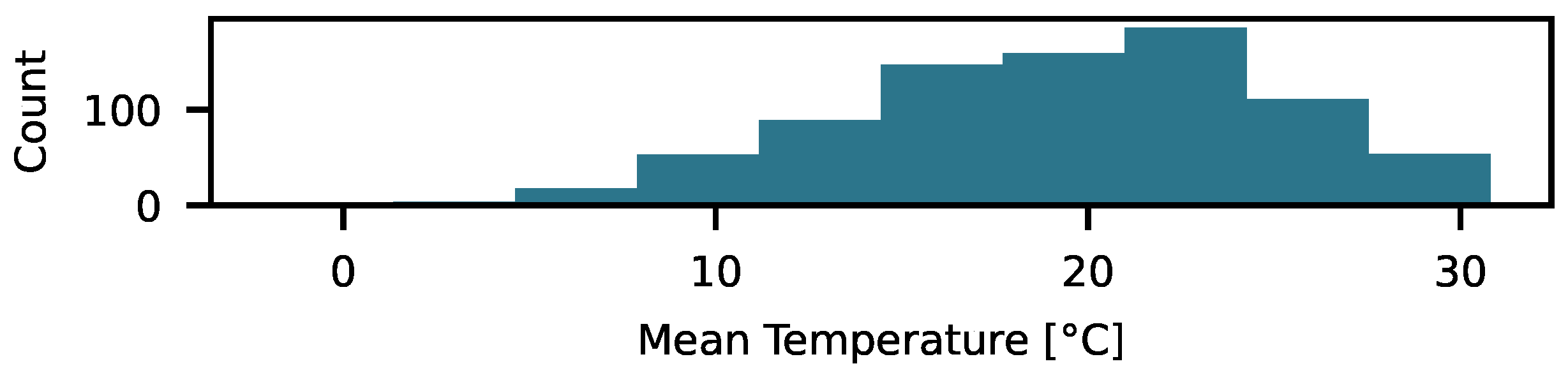
Figure 3.
The figure displays the flowchart of the general RPM and the introduced gradRPM.
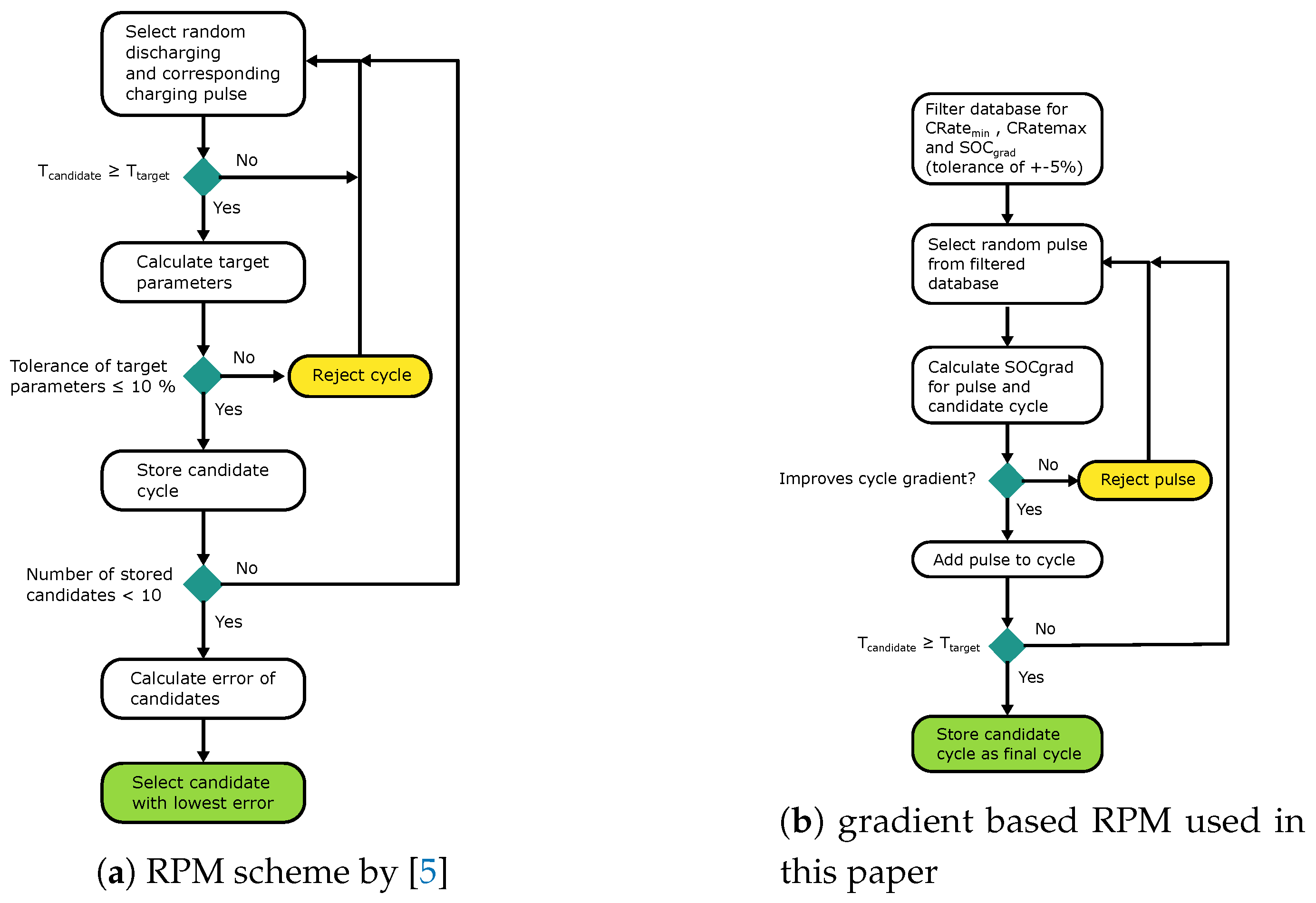
Figure 4.
Generated profile using the gradRPM and the corresponding change of the SOC in a sequence of control parameters
Figure 4.
Generated profile using the gradRPM and the corresponding change of the SOC in a sequence of control parameters
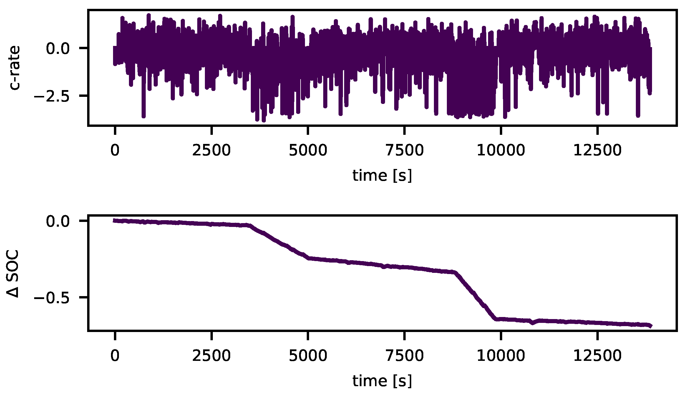
Figure 5.
Schematic of LTTB in (a) and an example of the output after the downsampling (b).
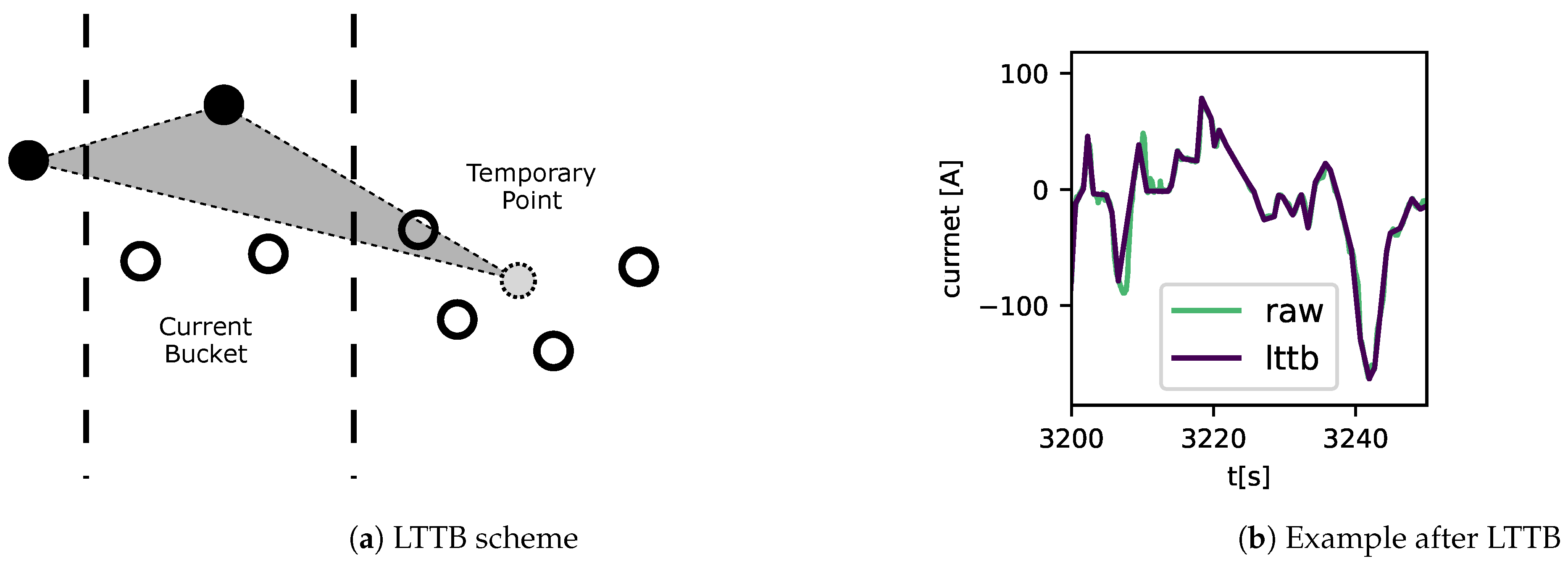
Figure 6.
Generative Adversarial Network.
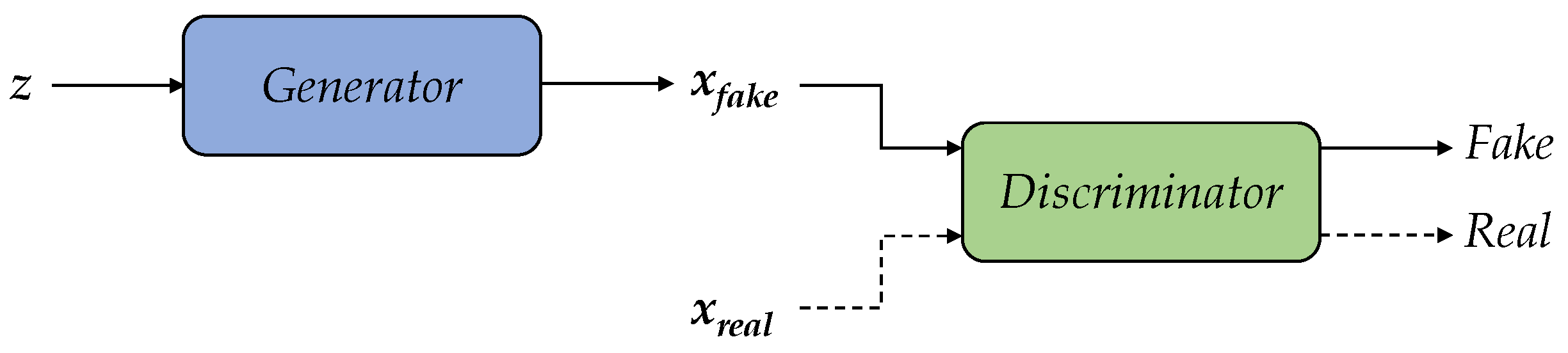
Figure 7.
The schematic diagrams of the three submodels: (a) generator scheme with synchronous sequence-to-sequence implementation, (b) discriminator scheme with sequence-to-class implementation, (c) conditioner scheme with sequence-to-class implementation.
Figure 7.
The schematic diagrams of the three submodels: (a) generator scheme with synchronous sequence-to-sequence implementation, (b) discriminator scheme with sequence-to-class implementation, (c) conditioner scheme with sequence-to-class implementation.
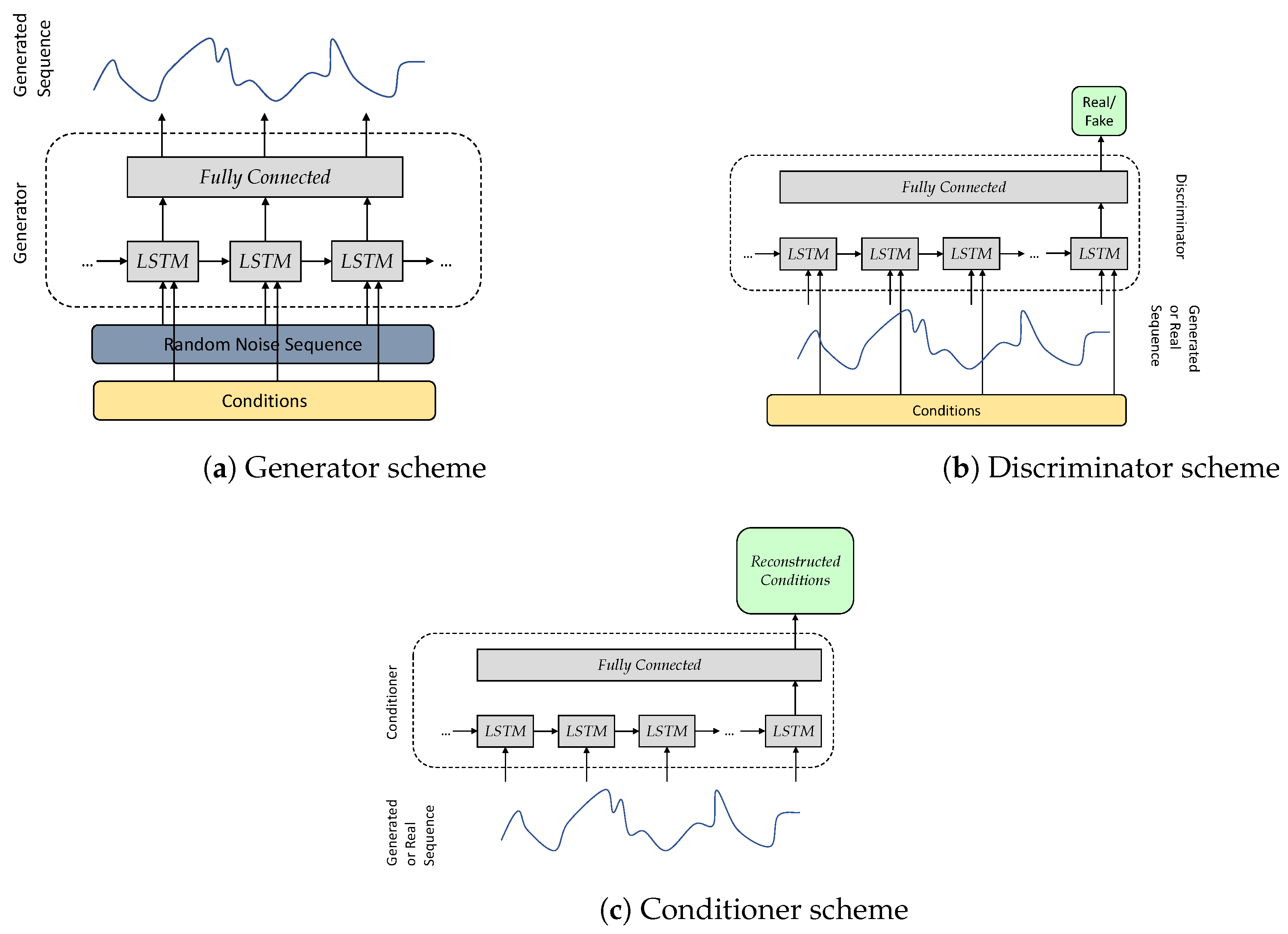
Figure 8.
Overall architecture of Info-RCGAN.
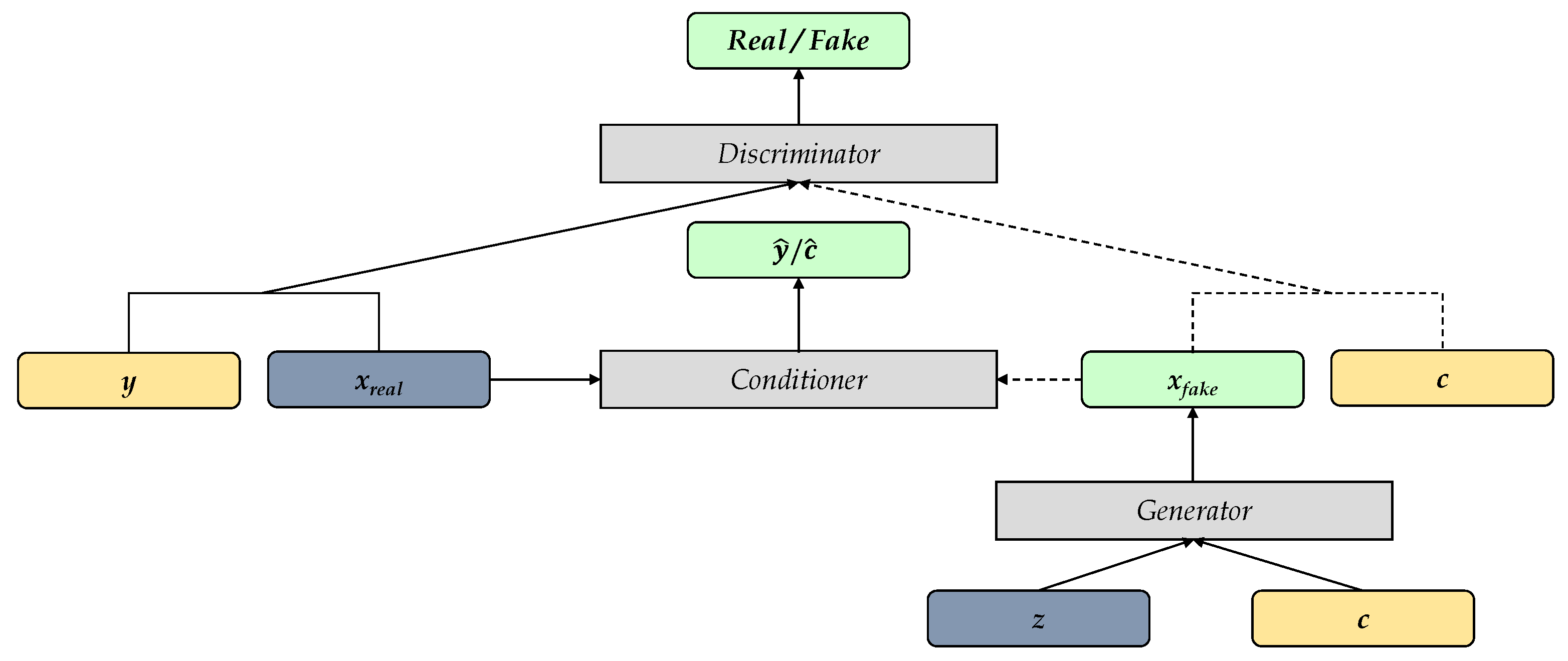
Figure 9.
The figure displays the cycles generated based on (a) the gradRPM method, (b) the Info-RCGAN, (c) the FUDS and (d) the DST. Subfigure (d) displays the histogram of C-rates of the different cycles with normalized counts.
Figure 9.
The figure displays the cycles generated based on (a) the gradRPM method, (b) the Info-RCGAN, (c) the FUDS and (d) the DST. Subfigure (d) displays the histogram of C-rates of the different cycles with normalized counts.
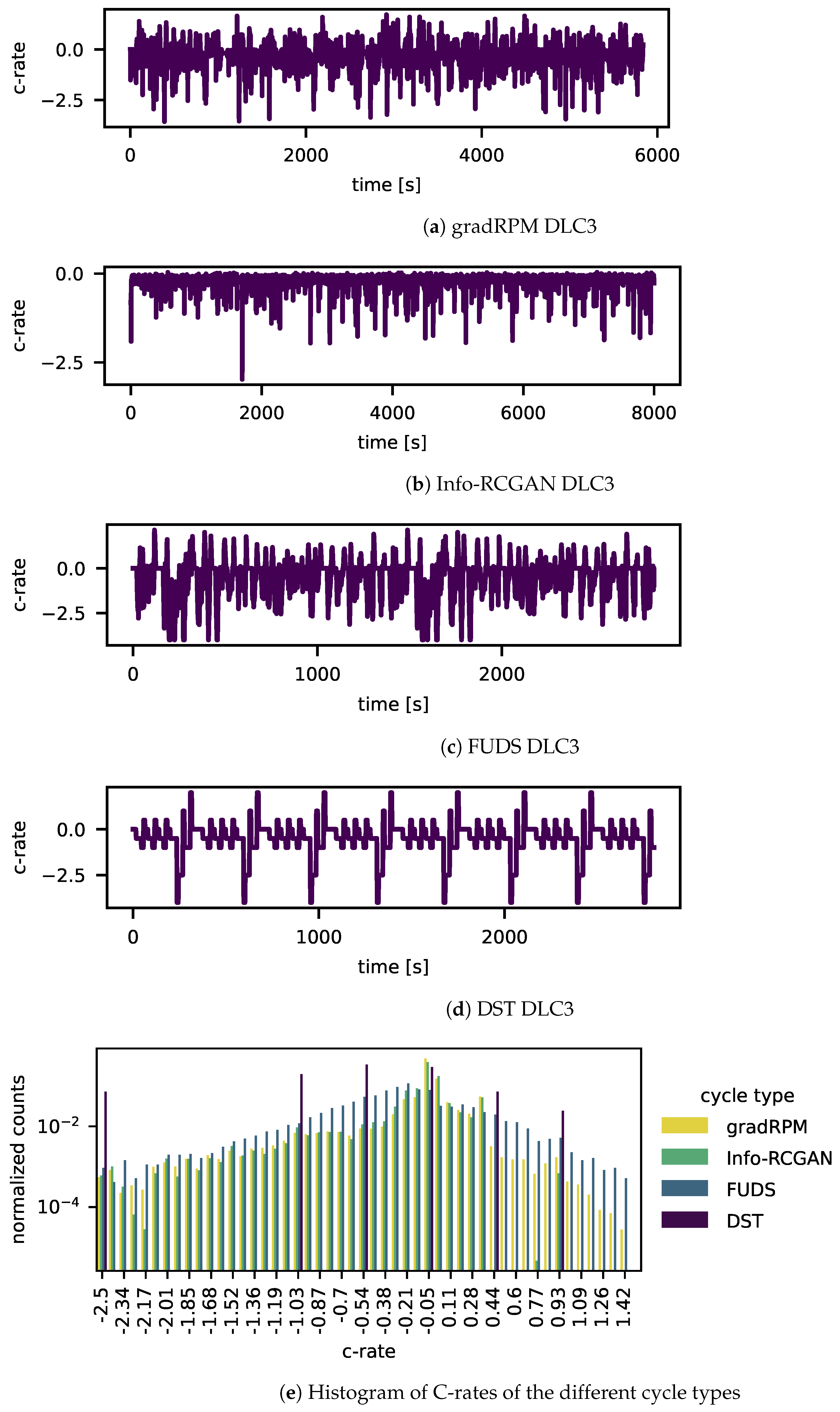
Figure 10.
The figure displays the different spectra of each data set in the columns from left to right of the BMW i3, the gradRPM, the Info-RCGAN and in the rows the analysed parameters from top to bottom the voltage, the C-rate and the temperature. Note the different scaling of the BMW spectra and the gradRPM and the Info-RCGAN spectra.
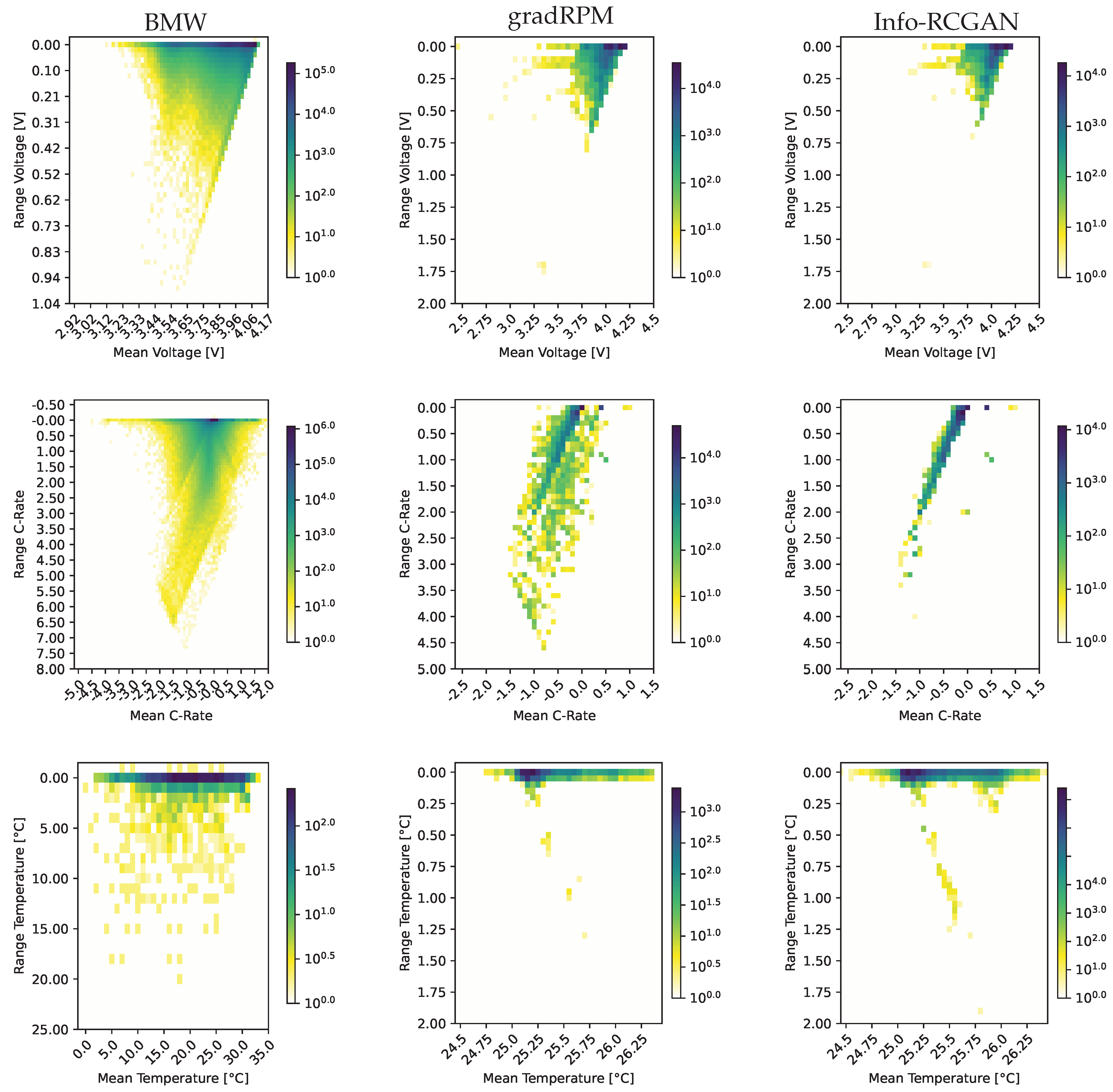

Table 1.
Parameters used for the ROM method.
| Parameter | Description | Type |
|---|---|---|
| Maximum C-rate accepted for load cycle | Control | |
| Maximum C-rate accepted for load cycle | Control | |
| Gradient of the SOC | Control | |
| The change of the SOC over the load cycle | Target | |
| T | Duration of the load cycle | Target |
Table 2.
Panasonic NCR18650GA.
| Characteristic | Value |
|---|---|
| Rated capacity | |
| Typical capacity | |
| Nominal Voltage | |
| Charging cut off voltage | |
| Charging current | |
| Discharging current | 10 |
Table 3.
Extracted and calculated design parameters for generating the dynamic load cycles (DLC) and the overall scenario based on expected 3 full cycle equivalents per day and a C-rate for constant current charging of 1 C
Table 3.
Extracted and calculated design parameters for generating the dynamic load cycles (DLC) and the overall scenario based on expected 3 full cycle equivalents per day and a C-rate for constant current charging of 1 C
| Dynamic Load Cycle ID | SOC Start | SOC end | Percent of the Scenario | Repetitions | Load Cycle Duration | SOC per h |
|---|---|---|---|---|---|---|
| DLC1 | 12 | 2520 | SOC/ | |||
| DLC2 | 30 | 1260 | SOC/ | |||
| DLC3 | 2 | 5040 | SOC/ |
Disclaimer/Publisher’s Note: The statements, opinions and data contained in all publications are solely those of the individual author(s) and contributor(s) and not of MDPI and/or the editor(s). MDPI and/or the editor(s) disclaim responsibility for any injury to people or property resulting from any ideas, methods, instructions or products referred to in the content. |
© 2024 by the authors. Licensee MDPI, Basel, Switzerland. This article is an open access article distributed under the terms and conditions of the Creative Commons Attribution (CC BY) license (http://creativecommons.org/licenses/by/4.0/).
Copyright: This open access article is published under a Creative Commons CC BY 4.0 license, which permit the free download, distribution, and reuse, provided that the author and preprint are cited in any reuse.


