Submitted:
27 May 2025
Posted:
28 May 2025
You are already at the latest version
Abstract
Rapid uptake of electric vehicles (EVs) in the Jawa–Madura–Bali (Jamali) grid produces highly variable charging demands that threaten supply–demand balance. To forestall instability, we developed a predictive simulation based on long short-term memory (LSTM) networks that combines historical generation and consumption patterns with models of EV population growth and initial charging‐time (ICT). We introduce a novel supply–demand balance score to quantify weekly and annual deviations between projected supply and demand curves, then use this metric to guide the machine-learning model in optimizing annual growth rate (AGR) and preventing supply demand imbalance. Relative to a business-as-usual baseline, our approach improves balance scores by 64% and projects up to a 59% reduction in charging load by 2060. These results demonstrate the promise of data-driven demand-management strategies for maintaining grid reliability during large-scale EV integration.
Keywords:
machine learning
; EV charging demand
; supply demand balance
; grid simulation
; Jamali power grid
; initial charging time
1. Introduction
The integration of electric vehicles (EVs) into Indonesia’s power grid presents both opportunities and challenges in achieving a sustainable and stable energy transition. While EV adoption contributes to reduced fossil fuel dependency and lower greenhouse gas (GHG) emissions, it also introduces new demand-side complexities to the electricity grid [1]. Unlike conventional loads, EV charging demand is highly intermittent, influenced by charging behavior, vehicle ownership trends, and urban traffic conditions. Without proactive supply-demand balancing, widespread EV adoption could lead to significant grid instability due to unsynchronized demand surges [2].
This study introduces a machine learning-based predictive simulation to model EV-driven demand growth within the Jawa-Madura-Bali (Jamali) power grid, Indonesia’s most heavily loaded electrical system [3]. The simulation forecasts supply-demand imbalances and recommends corrective actions to prevent demand overshoot while optimizing annual growth rate (AGR) and vehicle preference shifts. This simulation enables proactive grid planning, offering a data-driven approach for policymakers to align EV adoption with energy system constraints.
1.1. Jawa Madura Bali Power System
Indonesia's power system consists of several interconnected grids, which are vital for managing the diverse energy needs across the archipelago. The country’s grid infrastructure is divided into multiple regions, with major grids including Sumatra, Jawa-Bali, Kalimantan, Sulawesi, and Papua. Among these, the Jamali grid stands out as the largest and most significant, both in terms of capacity and demand [4].
The Jamali grid serves the densely populated Java Island, which is home to approximately 55% of Indonesia's population with most vehicles and hosts the capital city, Jakarta [5]. This high population density, coupled with economic activity, places considerable demands on the grid. Java island, being the most inhabited region in Indonesia, is central to the country's power system. The Jamali grid is an extensive interconnected system that manages both supply and demand across the islands of Java, Madura, and Bali. Historically, the Jamali grid has experienced significant growth in both supply and demand [6]. The demand has surged due to increasing urbanization, industrialization, and a rise in residential consumption, while the supply side has been driven by substantial investments in power generation and infrastructure upgrades.
In recent years, the Jamali grid has faced evolving challenges due to the growing integration of intermittent renewable energy sources and the increased demand from EV charging [7]. Historically, the grid has had to adapt to these changes, balancing the supply and demand dynamics while maintaining stability. The anticipated surge in EV usage is expected to further influence the grid's supply-demand balance. Understanding these historical trends and current developments is crucial for ensuring a stable and reliable power system for the future [8].
1.2. Jawa Madura Bali Grid’s Supply and Demand Historical Growth
The Jawa Madura Bali (Jamali) grid's supply side is supported by a network of diverse power plants, including thermal, hydroelectric, and increasingly renewable energy sources. As 2023, the Jamali grid comprises 402 power plants with a total installed capacity of around 48,000 megawatts (MW). This capacity is distributed among several large thermal power plants, including coal and gas-fired plants, as well as a growing number of hydro and solar installations [9]. The grid's supply capacity has seen consistent growth over the years, driven by ongoing investments and upgrades aimed at meeting the rising energy demand and incorporating more sustainable energy sources.
Figure 1 illustrates the historical growth in supply capacity for Indonesia’s power system (1974–2004), as reflected in the Jamali grid.
The peak demand has risen sharply; introducing EV fleets without corrective measures could further strain the balance. Table 1 presents the installed capacity and peak demand of the Jamali grid over the past ten years.
1.3. Development of Electric Vehicle Growth in Indonesia and the Impact on the Grid
The adoption of EVs in Indonesia is in its early stages but is set for significant expansion. As of 2023, the number of EVs in Indonesia ranges between 10,000 and 20,000, marking the beginning of a broader market development [10]. The Indonesian government aims to escalate this number to 2 million EVs by 2030 [11] through a variety of incentives. These include tax breaks, reduced import duties, and subsidies aimed at both EV purchases and the development of essential charging infrastructure.
Indonesia has implemented a range of regulations and incentives to promote the adoption of EVs as part of its strategy to address environmental and energy challenges. Key measures include the odd-even license plate policy in major cities like Jakarta, which restricts vehicle use based on license plate numbers on certain days to reduce traffic congestion and air pollution, thereby indirectly encouraging EV adoption [12]. Additionally, the government offers tax incentives, such as reduced import duties and exemptions from luxury goods taxes, making EVs more affordable and stimulating market growth [13]. Further incentives include free or discounted parking for EVs in some cities, which lowers the overall cost of ownership and enhances consumer appeal [14].
To support the expanding EV market, the government is also investing in charging infrastructure, with initiatives to install charging stations in public areas and along highways [15]. Additionally, the Indonesian government has introduced further subsidy programs to accelerate the transition to electric vehicles. These programs include a 10% VAT reduction for four-wheeled electric vehicles (4wEVs), as stipulated in Ministry of Finance Regulation No. 38 of 2023 [16], and a deduction of IDR 7,000,000 for two-wheeled electric vehicles (2wEVs), as detailed in Ministry of Industry Regulation No. 6 of 2023 [17]. The political landscape in Indonesia is a critical factor in shaping the growth of EVs within the country.
At present, the impact of EVs on the grid is relatively minor due to their limited numbers [18]. However, as EV adoption grows, particularly during peak charging periods, there will be increased demand on the grid.
1.4. Literature Review and Overview of Contributions
This study extends our earlier MDPI publication, Simulating EV Growth Scenarios in Jawa–Madura–Bali from 2024 to 2029: Balancing the Power Grid’s Supply and Demand, by integrating advanced machine learning methods to project grid dynamics through 2060.
Existing work on EV–grid integration has predominantly employed static supply–demand–coupled frameworks, exemplified by Song and Hu’s learning-based optimization of charging station locations for demand management [19] and Tang et al.’s dual-layer MPC for coordinated battery load demand and grid-side supply matching at swapping stations [20]. However, these static frameworks often underestimate peak deficits and overlook evolving temporal charging patterns, as demonstrated in comparative analyses of dynamic versus predetermined load scenarios.
To enhance forecast accuracy, recent studies have leveraged recurrent architectures—particularly long short-term memory (LSTM) networks—where Liu et al. developed a multiheaded convolutional LSTM model for green energy forecasting, improving solar irradiance and wind power predictions by over 25 % [21], and Eze and Ayorinde’s systematic review confirmed that LSTM-based approaches consistently outperform traditional methods, reducing forecasting errors by up to 30 % under variable conditions [22].
Additionally, the role of initial charging time (ICT) distributions in shaping aggregate EV demand has been quantified: Wang et al. used Monte Carlo simulation on charging-station order data to show that optimized ICT profiles can lower peak loads by 15–20 % [23], while Wan et al. introduced a model-free deep reinforcement learning scheduler that adaptively learns real-time strategies, achieving up to 20 % load flattening under dynamic pricing [24]. Collectively, these findings advocate for integrated frameworks that combine advanced LSTM forecasting with ICT-aware scheduling and reinforcement-learning control to ensure resilient and efficient EV–grid integration under rising penetration rates.
Building on these insights, the present study contributes to the field in five key ways:
- It introduces a machine learning–driven supply–demand balance simulation that dynamically adjusts EV charging profiles across multiple scenarios, replacing static assumptions with data-informed trajectories.
- It leverages LSTM networks to forecast long-term supply and demand growth, enabling the recommendation of corrective actions when projected demand growth threatens grid stability.
- It implements a suite of EV adoption scenarios—incorporating shifts in vehicle preferences, ICT optimization, and load-reduction strategies—to reflect plausible technology and behavioral trends.
- It develops a quantitative scoring system to evaluate grid stability under each scenario, thereby assessing the effectiveness of machine learning–informed interventions.
- It demonstrates that machine learning–based optimization of EV growth can significantly improve balance scores relative to business-as-usual projections, ensuring more reliable integration of electric vehicles into the Jawa–Madura–Bali grid.
Together, these contributions establish a robust, data-driven framework for evaluating policy and infrastructure strategies in support of Indonesia’s low-carbon transport transition.
1.5. Structure of the Paper
The remainder of this paper is structured as follows:
- Section 2 (Materials) details the machine learning methodology, data sources, and predictive modeling techniques used in the simulation.
- Section 3 (Methods) presents the supply-demand simulation framework, including demand growth factors, ICT modeling, and scenario configurations.
- Section 4 (Simulation Results) presents the Data sets for LSTM train, validate test, 2024 input, 2035 BAU output and the output 2060 (BAU and if corrective measures taken)
- Section 5 (Discussions) provides and discussions, comparing ML-predicted outcomes against BAU simulations and analyzing policy-driven impacts on grid stability.
- Section 6 (Conclusion) concludes with key insights, policy recommendations, and future research directions for EV integration in Indonesia’s power grid.
2. Materials
2.1. Understanding EV Intermittency
Electric Vehicle intermittency refers to the variability in energy demand from EVs due to factors like charging patterns and usage. Managing this intermittency is crucial for ensuring a stable energy supply and efficient grid operation. Following is a detailed overview that combines technical calculations with strategies for integrating EV demand.
As the number of EVs grows, total energy demand increases, especially during charging periods when energy consumption is at its peak. This rise in demand is particularly pronounced when many EVs charge simultaneously or during peak hours, leading to significant peaks in energy demand [7]. In the context of EVs, ICT refers to the Initial Charging Time, which is the time required to start charging the vehicle's battery from its current state [25]. The ICT is then projected to a weekly pattern for this simulation, as shown in Figure 3.
Figure 2.
ICT Probability.
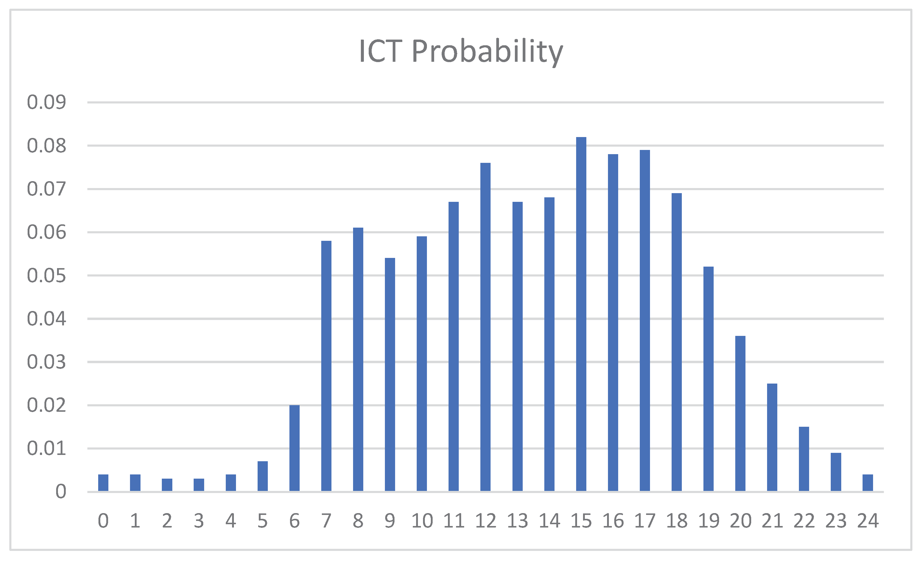
Figure 3.
Weekly ICT Probability.
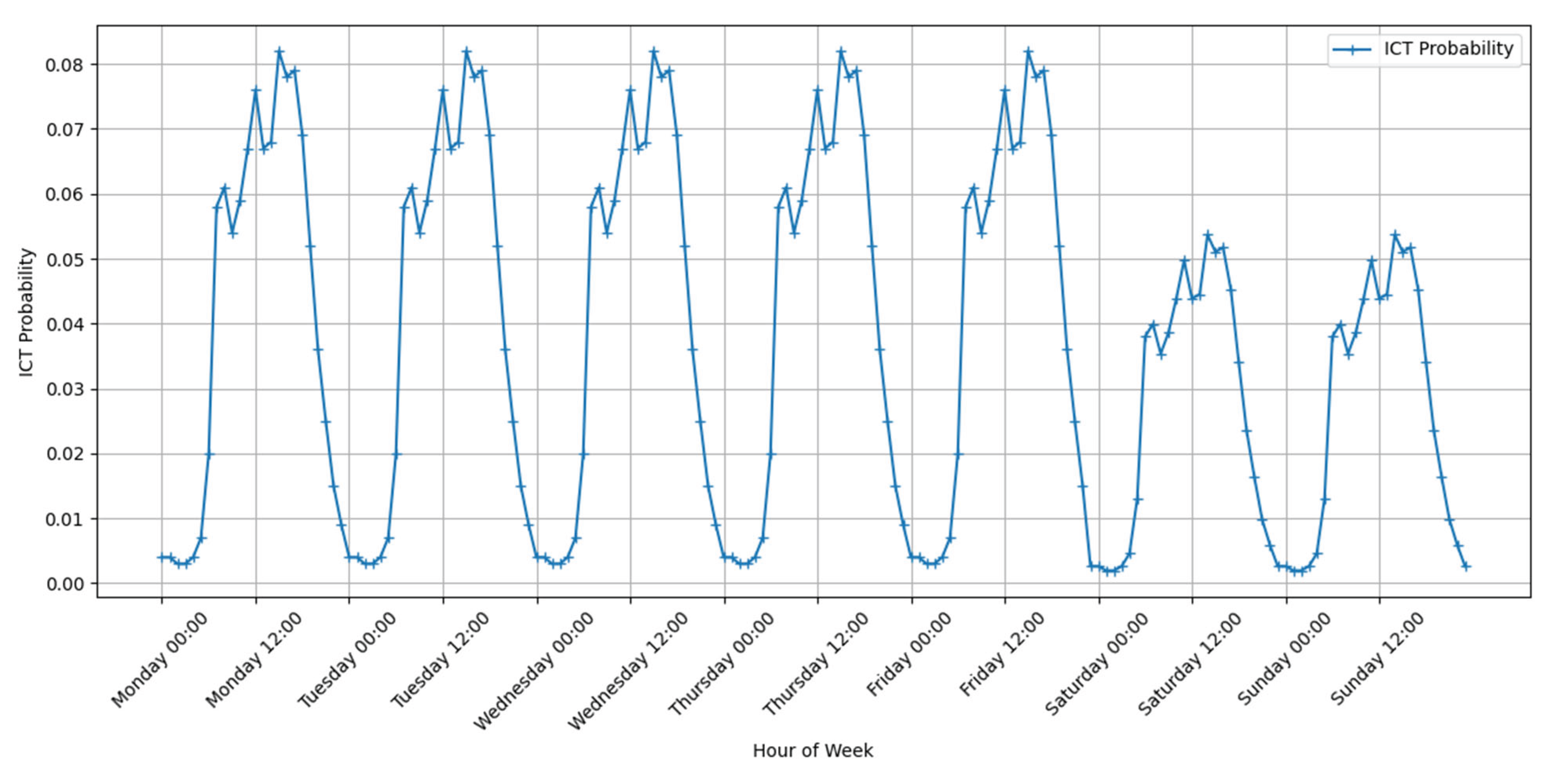
In the weekly EV charging demand simulation, the total charging load at each hour of the week (t=0, …, 167) is modeled as a convolution of the stochastic initiation of charging sessions ICT with per-vehicle charging power profiles, scaled by the fleet size and charging frequency, and partitioned into AC and DC charging components. Specifically, for each vehicle model i, the fleet size Ni was denoted, the average weekly session per vehicle
and the mode shares si,AC and si,DC defined by the AC:DC ratio, with
when DC capability exists, otherwise si,AC = 1. Let pICT(h) be the probability of session initiation at week hour h, and let Pi,m() for m ∈ {AC, DC} be the discrete power profile (kW) as a function of elapsed charging time (from the parsed times and power curves). The per-model, per-mode demand was calculated via
and the overall demand is then
with the AC and DC subcomponents obtained by restricting the inner sum to m = AC or m = DC. This formulation accurately captures the temporal distribution of charging events via ICT convolution, the heterogeneity of vehicle-specific power curves, and the influence of fleet composition and weekly charging frequency.
2.2. Machine Learning Methods
To forecast long-term grid dynamics in the Jawa–Madura–Bali system, we considered four principal families of time-series models: statistical ARIMA, kernel-based Support Vector Regression (SVR), ensemble Random Forest, and recurrent Long Short-Term Memory (LSTM) networks. Each approach offers distinct advantages and limitations when applied to multivariate, nonlinear hourly load data over multi-decadal horizons.
The Autoregressive Integrated Moving Average (ARIMA) model decomposes the series into autoregressive (AR) terms, differencing operations to enforce stationarity, and moving-average (MA) components. While ARIMA reliably captures linear temporal correlations in well-behaved, stationary series, its performance degrades in the presence of pronounced nonlinearities and exogenous interactions unless extensive feature engineering is undertaken.
Support Vector Regression (SVR) extends the SVM framework to regression by fitting a function within an ε-insensitive tube, leveraging kernel transformations to model nonlinear relationships. When configured on lagged input windows, SVR can mitigate noise and overfitting in high-dimensional settings. However, its reliance on fixed training horizons and the computational burden of kernel and hyperparameter selection limit scalability for long-range forecasting.
Random Forest regression constructs an ensemble of decision trees trained on lagged features and averages their outputs to reduce variance and control overfitting. This nonparametric, ensemble-based approach does not require stationarity assumptions and can capture nonlinear dependencies. Nevertheless, its fixed temporal window restricts memory of distant patterns, hindering the accurate modeling of seasonality and secular trends beyond the training window.
Long Short-Term Memory (LSTM) networks address these limitations by incorporating gated cell states that regulate information flow across time steps. An LSTM cell computes the following operations at each time step t [26]:
where:
- xt is the input vector at time t.
- W and U are weight matrices and bias vectors for the respective gates and candidate cell state.
- σ is the logistic sigmoid activation, and tanh is the hyperbolic tangent activation.
- ⊙ denotes element-wise multiplication.
This architecture prevents gradient vanishing or explosion, enabling the model to learn both short- and long-term dependencies. Given our objective to capture nonlinear interactions over a 36-year horizon, the LSTM network provides the most favorable trade-off between representational capacity and computational tractability.
3. Methods
3.1. Simulation Details
The simulation is implemented in Google Colab to leverage its free, cloud-based Python environment, which provides seamless collaboration, scalable compute resources, and straightforward integration with data storage services [27]. This choice ensures reproducibility and ease of access for all collaborators without the need for local software installations.
Simulation Periods: (change this to a table)
- ML_TRAIN (1974–2004): Historical data used to fit the machine-learning model parameters.
- ML_VALIDATE (2004–2014): Independent historical subset for hyperparameter tuning and overfitting assessment.
- ML_TEST (2014–2024): Final historical block to evaluate predictive performance prior to forecasting.
- BAU_SIMULATION (2025–2034): Business-as-usual projection of supply and demand under current policy and growth trends.
- ML_CORRECTION (2035–2060): Comparative scenario applying ML-derived adjustments to the BAU baseline to explore alternative outcomes.
These temporal boundaries (y-3 through yT) are configurable based on specific research and real-world conditions. The years are indexed by an offset yoffset ∈ {-3,-2,-1,-,1,…,X,Y}:
- y-3 corresponds to the first ML training year (1974)
- y-2 marks the first year of ML validation set (2004)
- y-1 marks the first year of ML testing year (2014)
- y0 denotes the last year of ML test-set (2024)
- y1 marks the first year of the BAU projection (2025)
- yx marks the final BAU year (2034), and
- yx+1 through yy cover the ML-corrected projection period (2035-2060).
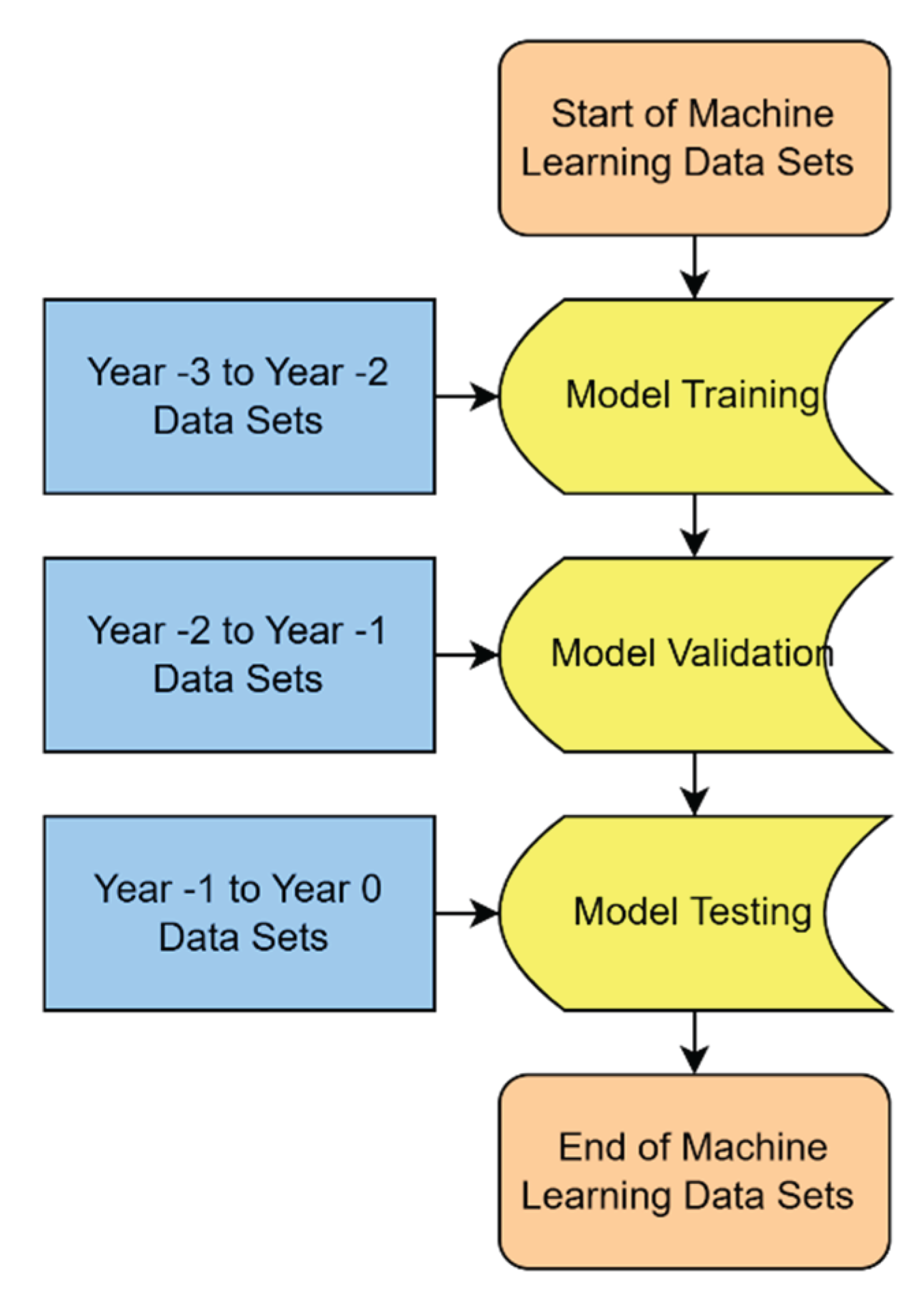
The simulation begins by training a Long Short-Term Memory (LSTM) network on historical Jamali grid data to capture annual growth patterns in both population-driven demand and PV supply capacity. Using the timeline offsets, the model undergoes sequential training, validation, and testing phases to ensure robust generalization. Once the LSTM has been calibrated, it produces an annual growth projection—namely, the expected percentage increase in EV charging demand and PV generation capacity for each forecast year.
Figure 4.
LSTM Simulation Flow.
3.2. Supply Demand Simulation
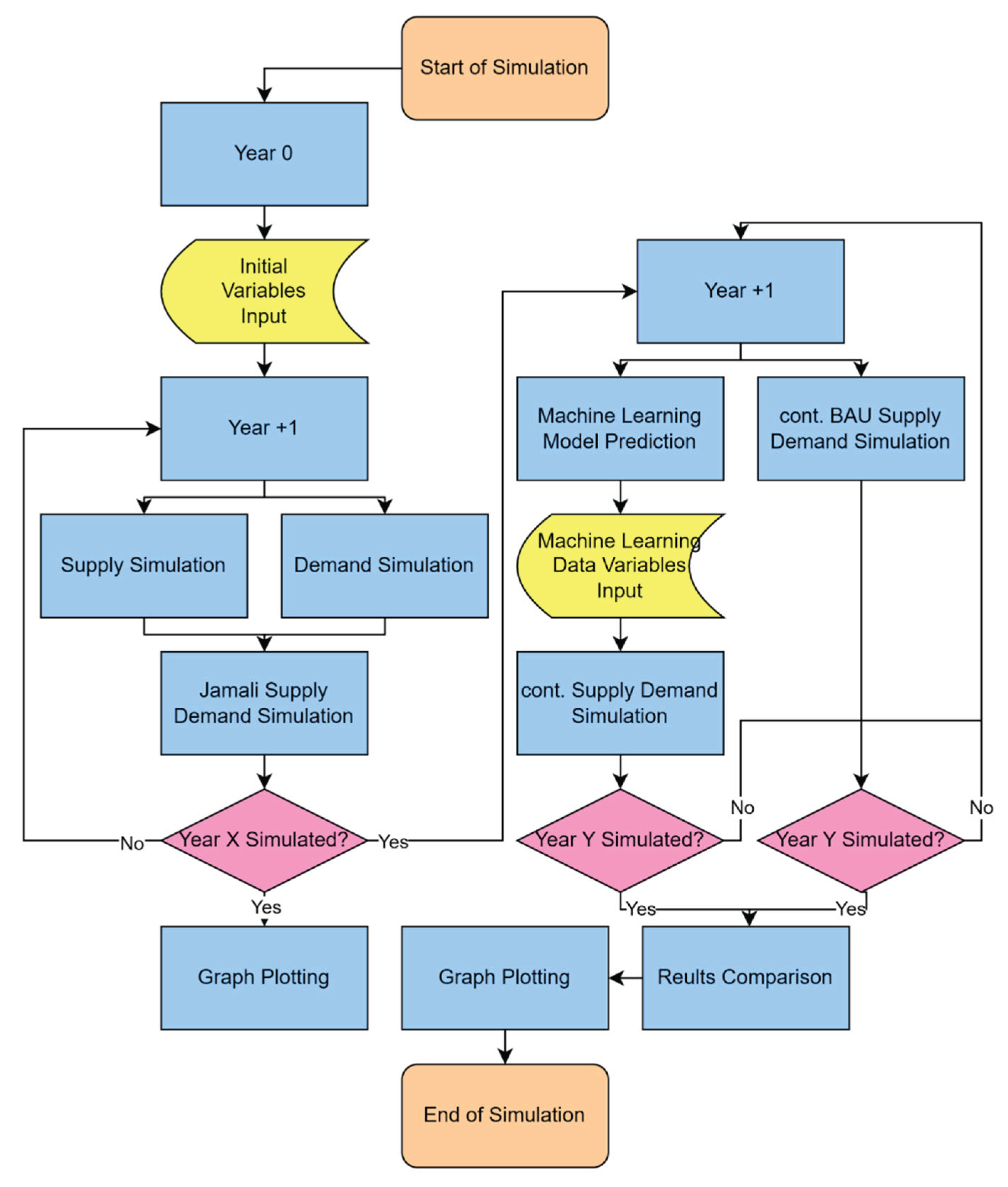
These LSTM-derived growth factors feed directly into the supply–demand balance module, which executes two serial workflows:
- Baseline (BAU) Simulation
- ML-Corrected Projection
Starting at Year 0 (y0), the model initializes all input variables (e.g., base supply curve, EV population, charging behavior parameters). For each subsequent year y, it computes hourly supply and demand curves, aggregates weekly energy balances, and advances to y+1 until the end of the BAU horizon yx. Upon completion, the results are plotted to visualize the evolving gap between generation and load.
Under the “business-as-usual” (BAU) assumption, current policy and investment trajectories remain unchanged through the end of the sitting president’s term [28]. Both supply and baseline demand curves continue to grow at their historical AGRs without any EV-related or corrective interventions. Balance Score are computed for each year to gauge how misalignment evolves if no new policies are adopted.
Beginning at Year yx+1, the simulation again steps through each year, but now adjusts the baseline supply and demand inputs using LSTM-predicted growth variables. This “corrected” pathway proceeds until yy, at which point the two result sets (BAU vs. ML-corrected) are overlaid for comparative analysis.
Figure 5.
Supply Demand Simulation Flow.
All computations and visualizations run in a Google Colab environment—Python 3.11 with TensorFlow 2.x, pandas, and NumPy—leveraging a standard Colab VM (Intel Xeon CPU, ~12 GB RAM, with optional Tesla T4 GPU). A full multi-decade simulation typically completes in 2–5 minutes on the default runtime.
3.3. Scoring System for Supply Demand Balance
The alignment between weekly supply St and total demand Dttotal are quantified via two complimentary metrics:
- Daily Energy Mismatch
- Shape Similarity via dynamic time warping (DTW)
The Daily Energy mismatch is computed using
Then the normalized root-mean-square error (NRMSE) in MWh:
and define the magnitude score Scoremag,t = 100% - NRMSEt.
The Dynamic Time Warping distance between St and Dttotal is
We normalize by DTW (S2024, S2024) to obtain
The final balance score for year t is the average:
3.4. Machine Learning and Simulation Accuracy Checks
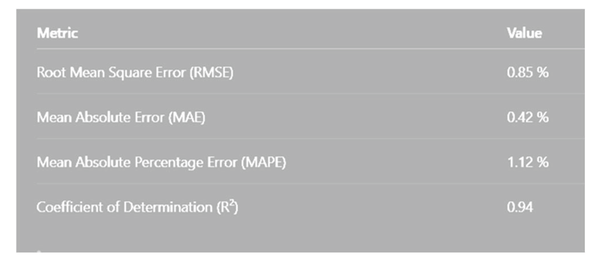
To assess the reliability of our LSTM-based growth forecasts, we evaluated model performance on the held-out ML_TEST dataset (2014-2024). Four standard error metrics were computed as shown in output graph of simulation below. [29]
Figure 6.
Simulation’s Output Error Metrics.
4. Simulation Inputs and Outputs
4.1. Machine Learning Data Sets (1974-2004)
Figure 7 shows the entire 1974–2024 series, mark the final LSTM prediction at 2024, and extend with the 10-year ahead forecast (2025–2034). This view emphasizes the continuity between model validation and long-term projection, and yields an average annual growth factor (multiplier) that feeds directly into our next supply–demand simulation stage
Walk-forward is the de facto standard in time-series forecasting competitions and operational deployments for robust model evaluation. It adapts the model to new patterns by retraining on each new observation, crucial for evolving grid supply dynamics. This method provides a realistic out-of-sample performance estimate to guide supply–demand simulation inputs. The final zoomed plot underscores how the model leverages recent data for reliable future growth estimation
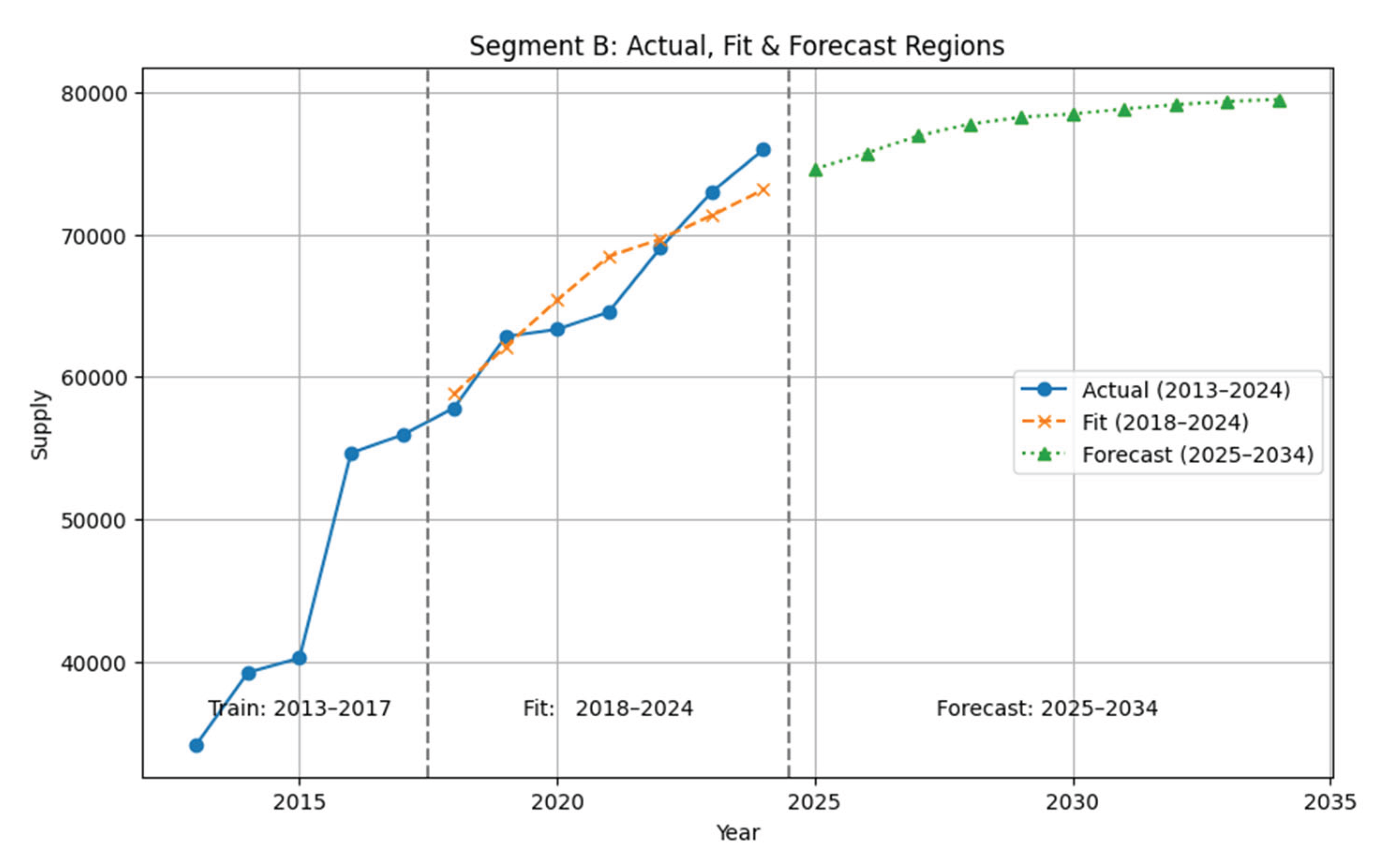
Zooming in on 2013–2024, this graph highlights the training window (2013–2017), the in-sample fit period (2018–2024), and the forecast horizon (2025–2034), clearly demarcated by vertical lines. It shows that the post-break LSTM adapts to the accelerated growth regime, providing a precise fit (MAPE ≈ 11 %) before projecting forward [29].
Figure 9.
Train, Fit and Forecast Region.
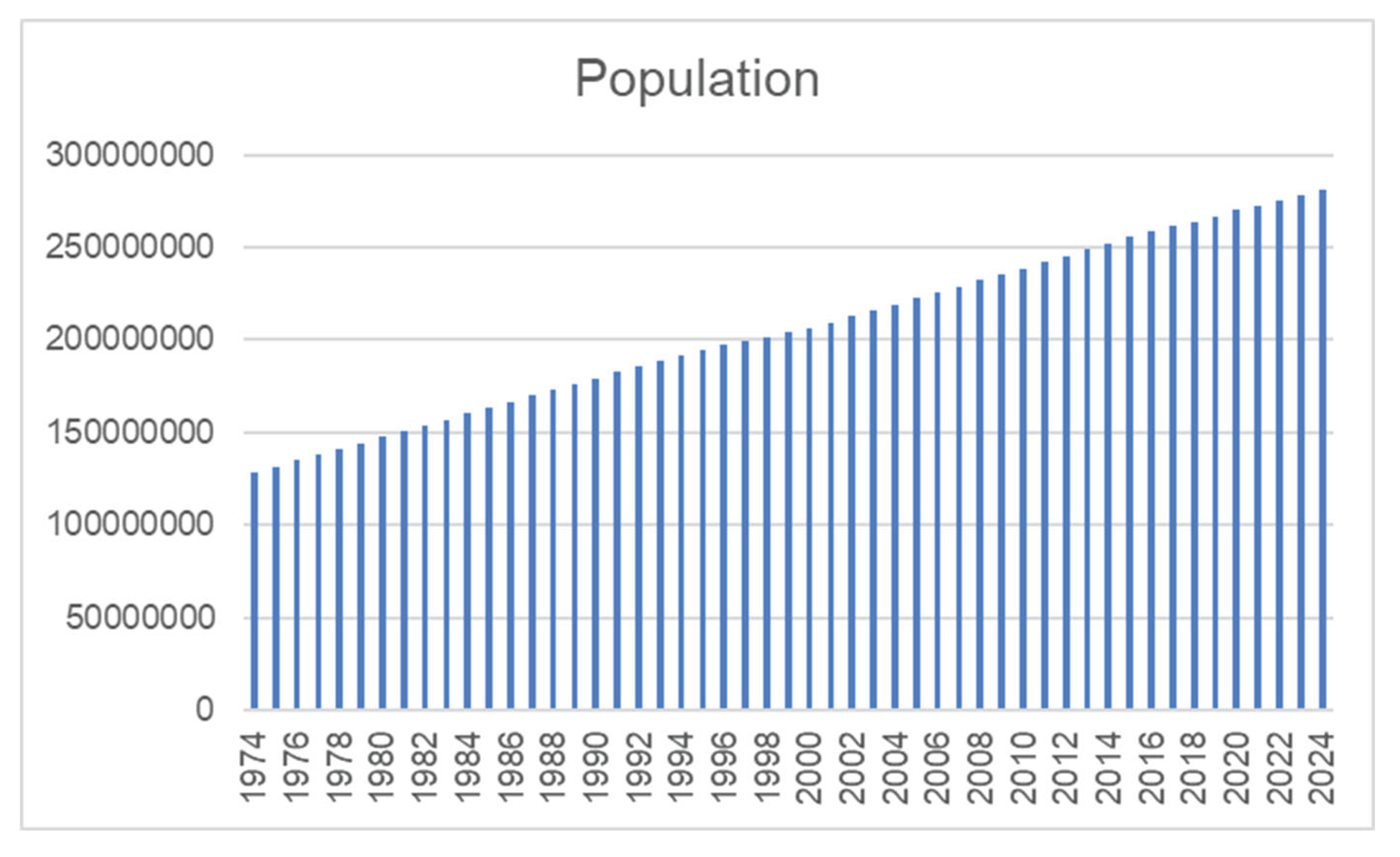
The population data is also being considered in the 1974-2024 data sets. The average is of 1,58% annual growth factor.
Figure 10.
Population Historical Data 1974-2024.
4.2. Beginning of Year0 (2024) Data Input
The data input could be categorized to 4 segments:
- Initial Variable Input and its AGR,
- Supply and Demand Curve in year 0,
- Vehicle Data and
- Vehicle Charge Load
The initial variable inputs are described in Table 2. The annual growth rate (AGR) is displayed in Figure 11.
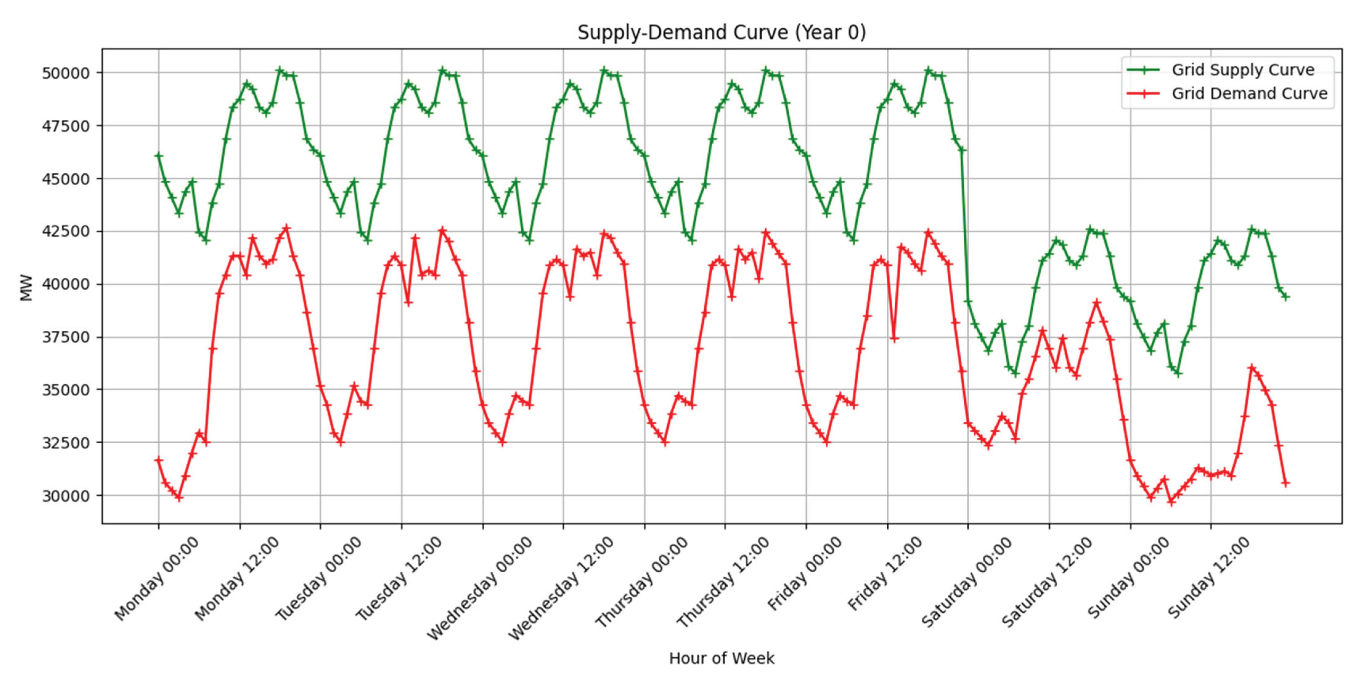
The baseline supply and demand curves for each simulation year were derived from peer-reviewed data and our prior MDPI publication, then adjusted using PLN Statistics for 2024 to ensure consistency with actual grid performance [37,38,39,40]. These weekly profiles represent one typical week of the Jawa–Madura–Bali grid’s supply–demand balance, reflecting diurnal and weekday–weekend variation without seasonal bias, given the region’s equatorial climate. National holidays and weekends induce discernible troughs in both supply and demand, as illustrated in Figure 13. In the initial year (year 0), the combined supply and demand profile (Figure 14) demonstrates lower power levels during weekend hours; this composite curve forms the reference state from which subsequent annual growth and corrective scenarios evolve.
Figure 12.
Supply Curve 2024.
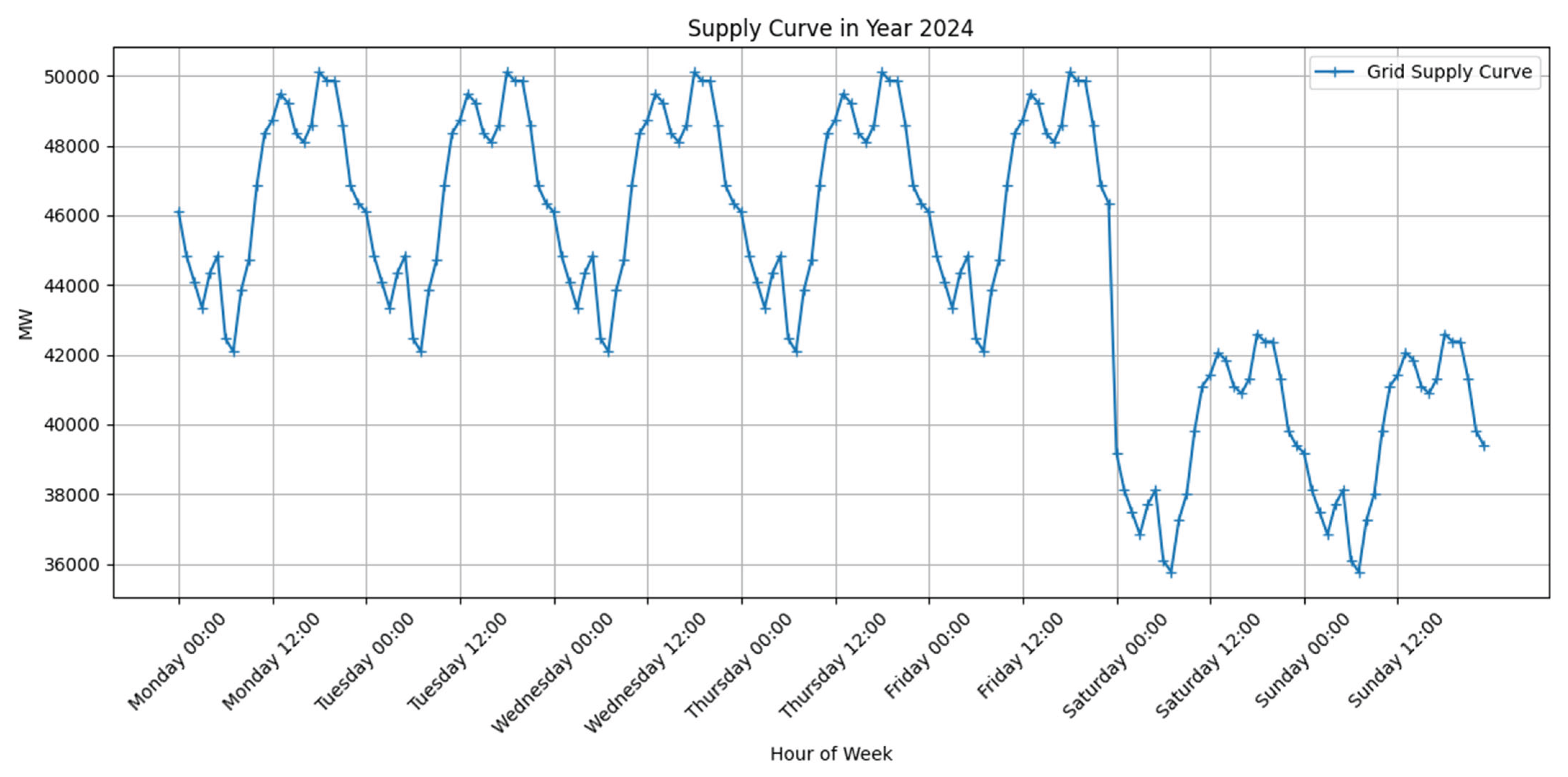
Figure 13.
Demand Curve 2024.
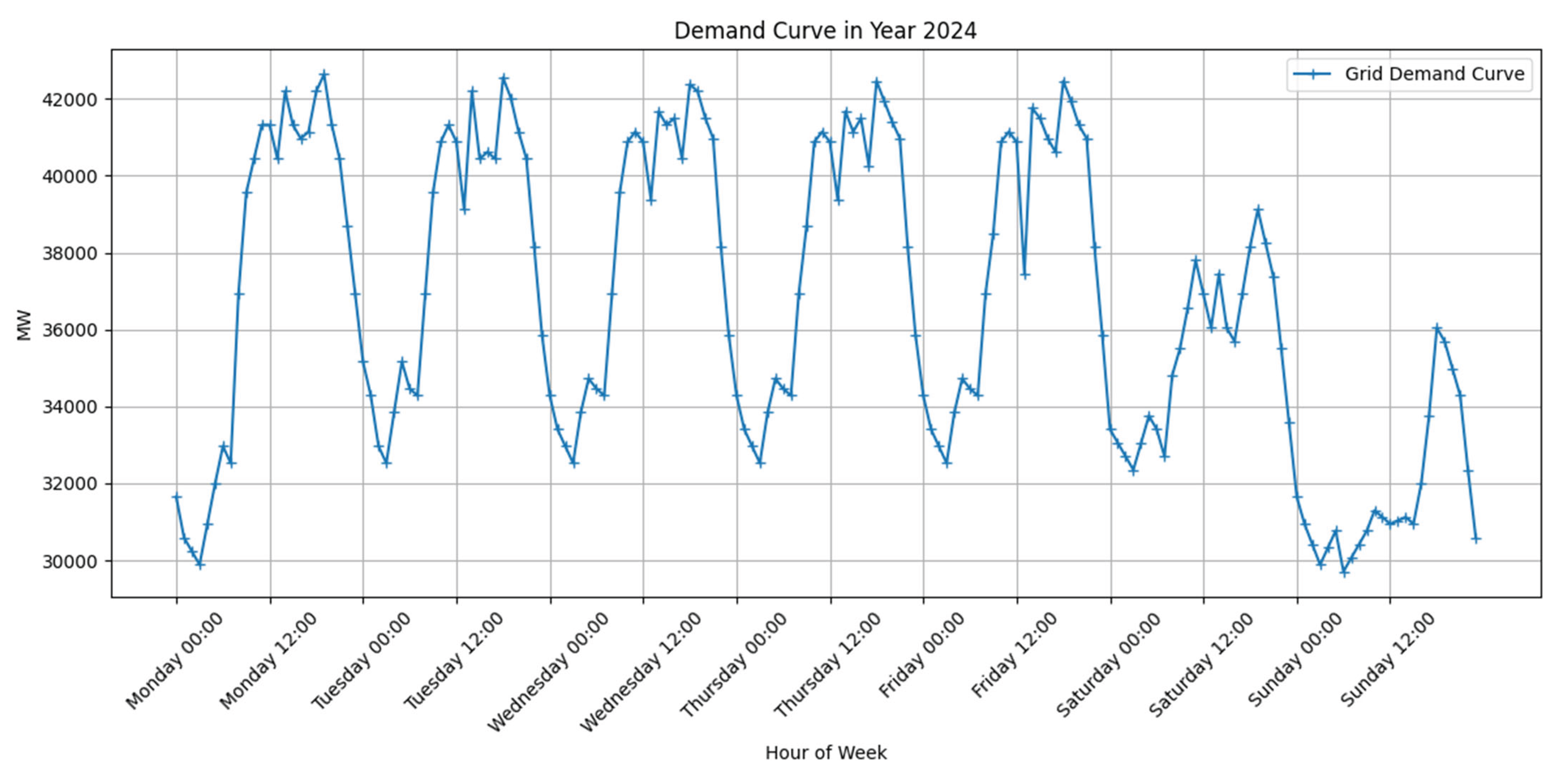
Figure 14.
Supply Demand Curve 2024.
The weekly ICT profile, shown in Figure 15, represents the probability that an EV begins charging at each hour of a typical week. This distribution was derived from national driving-pattern surveys [25] and reflects higher charging start probabilities during end of the day evening, with reduced likelihood during work hours and weekends.
Below is a summary of the eight electric-vehicle models included in our simulation, spanning both passenger cars and two-wheelers. For each vehicle we specify its nominal driving range (200–620 km), battery capacity (1.44–103 kWh), DC-fast-charging capability (where available), typical charge duration for both DC and AC modes, peak charging power, assumed days between charges (30 days), and the year production began. These parameters form the basis of our charging-load profiles and directly feed into the demand-side modelling. [41,42,43,44,45,46,47,48,49,50]
The table below lists the EV models included in our simulation, chosen for their market popularity and representative features. We apply a price-based classification to distinguish daily-use from luxury vehicles: any four-wheeler priced below IDR 400 million or two-wheeler priced below IDR 30 million is treated as a daily-oriented model in this study, while those above these thresholds are considered luxury segment examples [51]. This categorization informs scenario definitions and ICT parameter assignments.

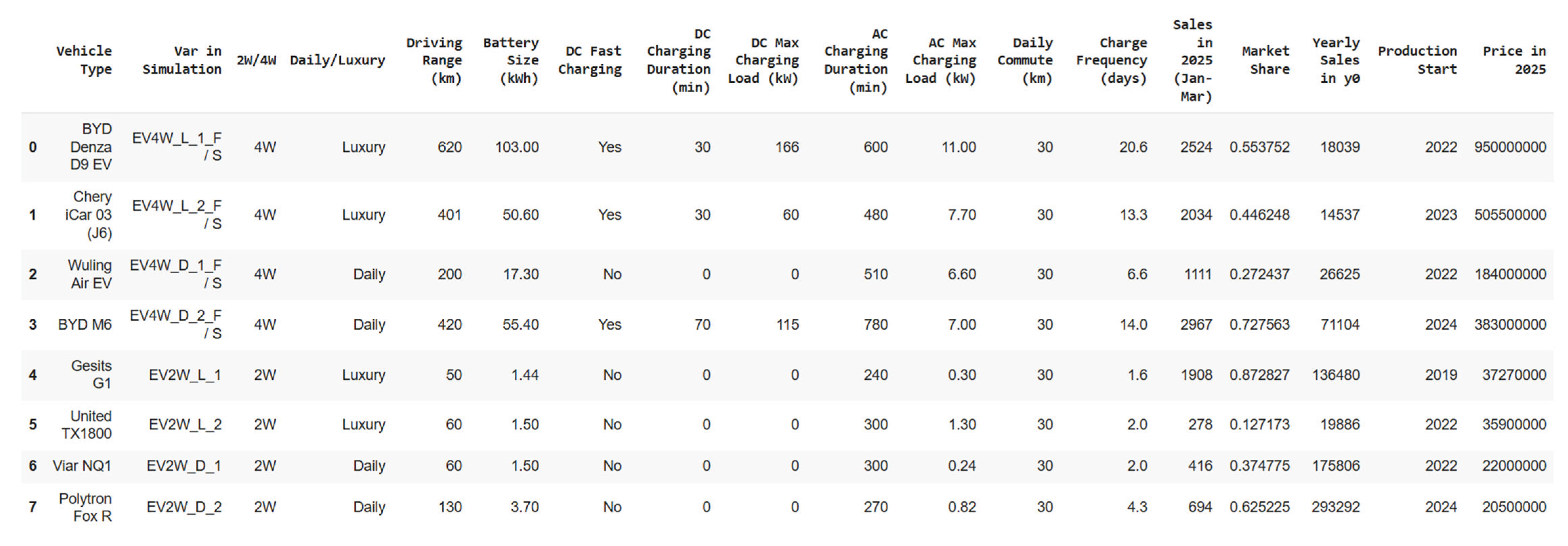
Figure 16 illustrates the charging power profiles used as inputs for our simulation, distinguishing between slow (AC) and fast (DC) charging modes according to a prescribed ratio—vehicles without DC capability are modeled as charging at AC 100 % throughout. The upper panels plot instantaneous charging power (y-axis) against state of charge (SOC, x-axis) for a representative set of vehicles: the left shows AC curves peaking between 0.5 and 11 kW, the right DC curves reaching up to 170 kW. These generic SOC-based charge curves—adopted in lieu of proprietary data and without accounting for battery-health effects—provide a reasonable first-order approximation of real behavior. The lower panels reframe the same profiles over charging duration (hours on the x-axis): the left for AC, the right for DC. Here, the pronounced variation in power over time highlights how load intermittency is driven by vehicle class and by the timing of charging initiation—key factors in assessing the temporal clustering of EV demand on the grid.
4.3. End of 2024 Simulation Output
Once all input parameters are specified, the year 0 simulation calculates the baseline EV population for each model. Using initial market share estimates, sales forecasts for 2025 (January–March), and the regional total vehicle stock, the algorithm allocates the number of units per model. Figure 17 presents a snapshot of the simulation output, displaying the computed vehicle counts by model that form the starting fleet for subsequent charging and load analyses.
Following initialization, the simulation calculates EV charging demand for each model over the reference week. Figure 18 presents the per-model demand results, while Figure 19 differentiates between AC and DC charging profiles, applying the power-duration curves described earlier. These tables quantify hourly load contributions from each vehicle type, combining ICT start probabilities with model-specific charging rates to form the aggregate EV demand input for the first simulation year.
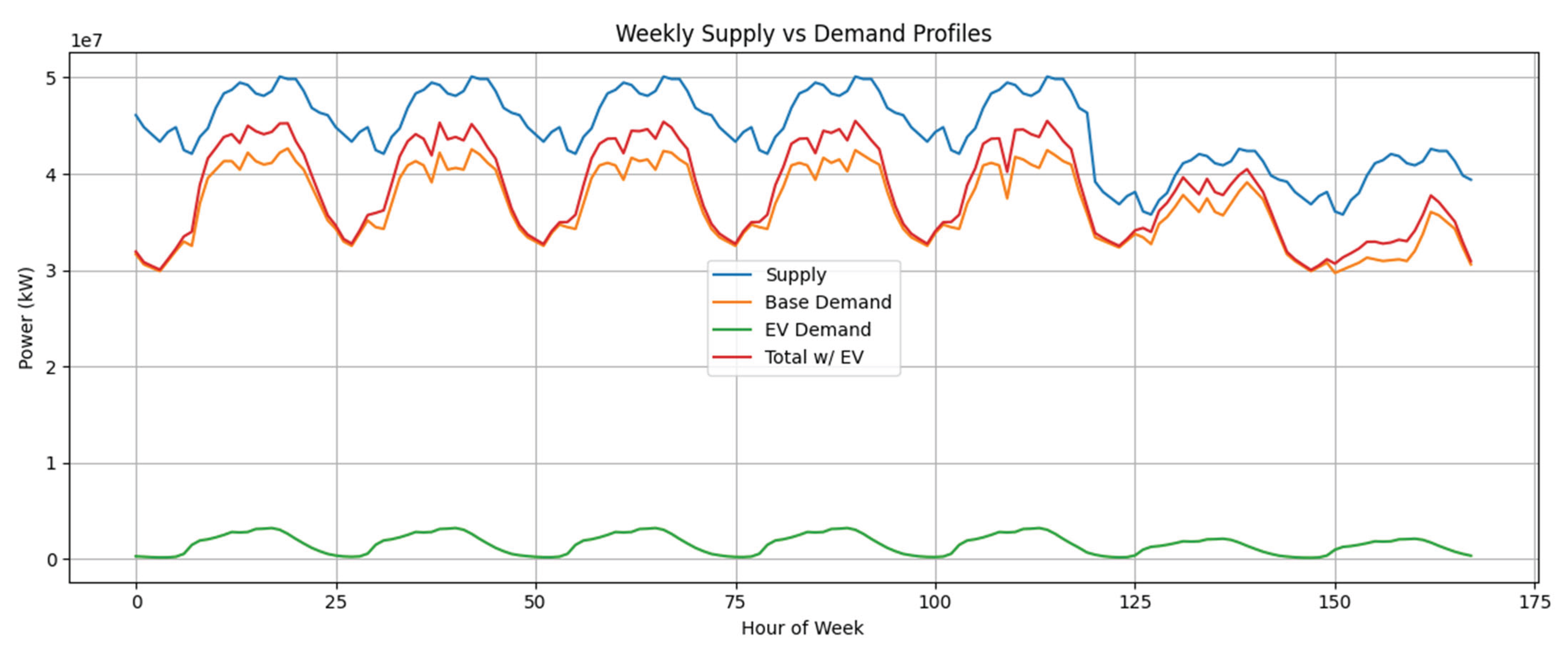
The aggregated EV demand profile is subsequently superimposed on the baseline system demand—comprising residential, commercial, and industrial loads—to produce the total load curve for year 0, displayed in graph 20
Figure 20.
Combined Supply and Demand Curves.
The hourly balance score is defined as the percentage ratio of supplied energy to demanded energy at a given hour. The weekly average balance score is then obtained by averaging the 168 individual hourly scores. Figure 21 illustrates both the hourly balance profile and its weekly mean, highlighting periods of surplus and deficit that inform corrective-action decisions.
To complement the weekly analysis, we compare daily supply and demand energies to reveal intraday mismatches. Figure 22 presents the total 24-hour supply–demand profile for the reference week in year 0.
4.4. 2035 BAU Output
After establishing the initial conditions, we simulate a business-as-usual (BAU) scenario over the next five years, aligning with the national presidential term length. This five-year buffer accounts for the lead time required to translate measurement insights into policy and infrastructure changes. As shown in Table Y, the grid balance remains robust throughout this period, indicating that current growth rates do not immediately compromise reliability.
Figure 23 compares the weekly balance scores for year 0 and year 5 under BAU, while Figure 24 presents the corresponding daily energy supply–demand profiles. Both visuals confirm that, even without corrective measures, the system sustains adequate performance over the first term.
Figure 25 further demonstrates that the weekly average balance score steadily increases over the 5-year BAU simulation horizon. This trend occurs because supply and demand trajectories become more closely aligned over time, reflecting the effect of consistent growth rates and the scaling of generation capacity in line with rising consumption.
4.5. 2060 BAU Output
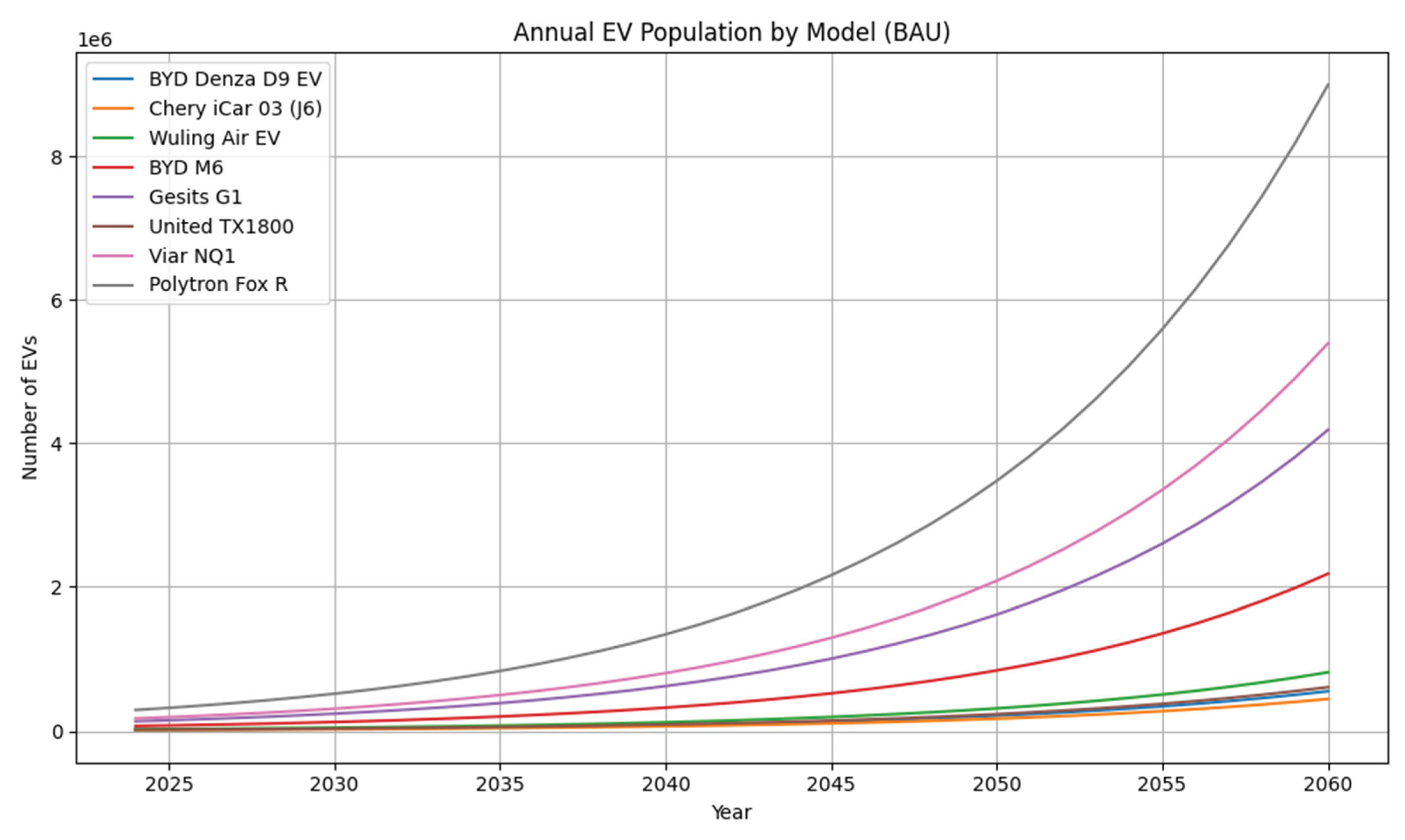
Extending the BAU simulation through to year 2060 reveals a pronounced divergence between supply and demand trajectories. Figure 26 illustrates the weekly balance comparison for year 0 and year 2060, highlighting substantial deficits during peak hours. The corresponding daily energy profiles (Figure 27) underscore severe shortfalls in the evening charging window, driven by the aggregate growth of the EV fleet (Figure 28). This gap originates from exponential increases in charging demand without proportionate expansion of generation capacity, indicating that the current BAU growth assumptions will render the grid unable to meet demand by 2060 without intervention.
Figure 28 depicts the projected population growth of each EV model under the BAU scenario, with separate curves for every vehicle type from the initial year through 2060. These trajectories reflect model-specific adoption rates and illustrate how the expanding fleet contributes to the escalating charging demand.
Figure 28.
Annual EV Population BAU.
4.6. 2060 Optimized Output
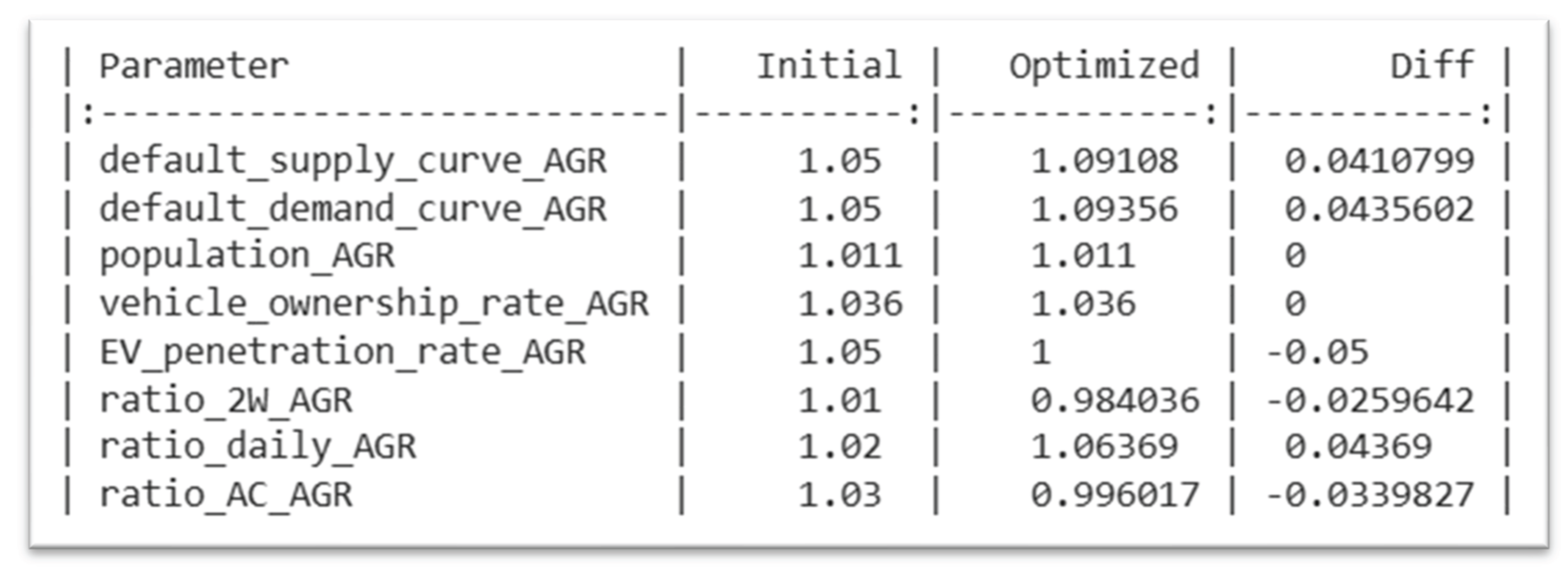
The simulation then applies the corrective actions recommended for 2035 to project grid performance through to 2060. Table 29 summarizes the initial annual growth rate (AGR) settings alongside the optimized AGR values suggested by the model—derived by minimizing projected supply–demand deficits—and the percentage difference between them. These adjustments indicate the precise scaling of demand and supply growth to implement in 2035, yielding the best system balance by 2060. By comparing BAU and optimized AGRs, stakeholders can identify which parameters require tightening or relaxation to prevent the large deficits observed in the unconstrained scenario.
Figure 29.
Optimized AGR.
If these corrective measures are fully implemented in 2035, the annual balance score under the optimized scenario steadily surpasses that of BAU. Figure 30 illustrates that by 2038 the optimized trajectory yields a higher average weekly balance, marking the first divergence where BAU underperforms. Furthermore, Figure 31 demonstrates that by 2042 the daily supply–demand gap in the BAU simulation expands sharply, indicating a critical loss of equilibrium. In contrast, the optimized scenario maintains manageable deficits, confirming the long-term efficacy of the 2035 interventions in preserving grid stability.
Figure 32 presents the stark contrast in weekly balance scores for the year 2060 between the BAU and optimized scenarios. In the zoomed inset of this diagram, the model’s effort to tightly align supply and demand is evident—particularly around hour 125 of the week—where the optimized curve closely tracks the supply profile, minimizing deviations that would otherwise appear under the BAU trajectory.
Figure 34 presents the aggregate 24-hour energy provided and consumed for year 2060 under both BAU and optimized scenarios. In the zoomed inset of Figure 35, the daily energy difference in the optimized scenario remains minimal.
This annualized energy difference translates into significant cost savings. Beginning in 2035 and extending through 2060, the optimized scenario contributes cumulative savings of approximately IDR 16,435 billion, as illustrated in Figure 36. (BPP PLN Rpxx [52])
Figure 37 further demonstrates that the simulation can track the growth rate of each EV model under optimized AGRs. From 2035 onward, individual vehicle trajectories deviate from the BAU path, reflecting the corrective AGR adjustments.
5. Discussion
The simulation outcomes for the 2060 planning horizon indicate that imposing a constraint on EV charging demand growth—ensuring its annual growth rate remains at or below the supply AGR from 2035 onward—yields substantial system-wide benefits. Under this corrective action, cumulative energy savings reach approximately 12 TWh by 2060, corresponding to avoided generation costs of roughly IDR 16,435 billion (based on an assumed average production cost of IDR 1,300/kWh).
Deferral of these measures until 2047 reduces energy savings to 5 TWh, lowers cost savings to IDR 3,500 billion, and degrades the grid’s average hourly balance score by 8 percentage points. These findings highlight the compounding advantage of early intervention: delays exacerbate supply–demand mismatches and necessitate more aggressive, capital-intensive capacity expansions in later years.
Achieving the required alignment by 2035 involves coordinated deployment of demand-side management, vehicle preferences incentives, and adaptive capacity planning of EV population.
6. Conclusion
This study presents a comprehensive simulation framework for the Jawa–Madura–Bali grid that integrates vehicle charging demand growth, business as usual growth rate and policy interventions through 2060. The simplification of modeling charging as a full 0–100 percent state-of-charge cycle enables clear quantification of aggregate demand impacts; future work should refine this assumption by incorporating more accurate represent partial-charge behavior.
The framework omits explicit representation of charging infrastructure costs and spatial availability, excludes V2G impacts on battery degradation, and assumes homogeneous driving and charging patterns across the region. Addressing these limitations in subsequent research—by integrating infrastructure investment models, spatially resolved travel behavior, stochastic renewable generation, and targeted regulatory scenarios—will further enhance the realism and policy relevance of the approach. Ultimately, this work underscores the critical role of early, integrated policy alignment in delivering energy, economic, and reliability gains during the transition to a decarbonized transport sector.
Supplementary Materials
Phyton Simulation Scripts.
Author Contributions
Conceptualization, J.V.T. and R.D.; methodology, J.V.T. and R.D.; software, J.V.T.; validation, J.V.T. and R.D.; formal analysis, J.V.T. and R.D.; investigation, J.V.T. and R.D.; resources, J.V.T. and R.D.; data curation, J.V.T.; writing—original draft preparation, J.V.T.; writing—review and editing, J.V.T.; visualization, J.V.T.; supervision, R.D.; project administration, R.D.; funding acquisition, R.D. All authors have read and agreed to the published version of the manuscript.
Funding
This research received no external funding.
Data Availability Statement
The original contributions presented in the study are included in the article, further inquiries can be directed to the corresponding author.
Conflicts of Interest
The authors declare no conflicts of interest.
Abbreviations
The following abbreviations are used in this manuscript:
| AGR | Annual Growth Rate |
| BAU | Business as Usual Scenario |
| DTW | Dinamic Time Warping |
| ICT | Initial Charging Time |
| GHG | Greenhouse Gases |
| Opt. | Optimized Scenario |
| 2W | 2-wheeler |
| 4W | 4-wheeler |
References
- Hawkins, T. R.; Singh, B.; Majeau-Bettez, G.; Strømman, A. H. Comparative Environmental Life Cycle Assessment of Conventional and Electric Vehicles. Journal of Industrial Ecology, Wiley 2012, pp 53-64. [CrossRef]
- Clement-Nyns, K.; Haesen, E.; Driesen, J. The Impact of Charging Plug-In Hybrid Electric Vehicles on a Residential Distribution Grid. IEEE Transactions on Power Systems 2010, Vol 25, pp 371-380. [CrossRef]
- Günther, M. Challenges of a 100% Renewable Energy Supply in the Java-Bali Grid. International Journal of Technology 2018, Vol 9, pp. 258. [CrossRef]
- Institute for Essential Services Reform (IESR). A Roadmap for Indonesia’s Power Sector: Toward 100% Renewable Energy?; IESR: Jakarta, Indonesia, 2019; pp. 18.
- Badan Pusat Statistik. Jumlah Penduduk Menurut Provinsi di Indonesia (Ribu Jiwa), 2024; BPS: Sulawesi Utara, Indonesia, 2024.
- Tumiran; Putranto, L.M.; Sarijaya; Pramono, E. Y. Maximum penetration determination of variable renewable energy generation: A case in Java–Bali power systems. Elsevier-Renewable Energy 2021, Vol 163, pp 561-570. [CrossRef]
- Damanik, N; Saraswati R; Hakam D. F.; Mentari, D. M. A Comprehensive Analysis of the Economic Implications, Challenges, and Opportunities of Electric Vehicle Adoption in Indonesia. MDPI Energies 2025, Vol 18(6), pp.1384. [CrossRef]
- Aldossary, M.; Alharbi, H. A.; Ayub, N. Optimizing Electric Vehicle (EV) Charging with Integrated Renewable Energy Sources: A Cloud-Based Forecasting Approach for Eco-Sustainability. MDPI Mathematics 2024, Vol 12(17), 2627. [CrossRef]
- Ministry of Energy and Mineral Resources (MEMR), Indonesia. Handbook of Electricity Generation Statistics 2023; MEMR: Jakarta, Indonesia, 2023.
- The Association of Indonesia Automotive Industries. Indonesian Automotive Industry Data 2023; Jakarta, Indonesia, 2024.
- Pemerintah Pusat. Peraturan Presiden (Perpres) Nomor 79 Tahun 2023 tentang Perubahan atas Peraturan Presiden Nomor 55 Tahun 2019 Tentang Percepatan Program Kendaraan Bermotor Listrik Berbasis Baterai (Battery Electric Vehicle) untuk Transportasi Listrik; Jakarta, Indonesia, 2023.
- Pemerintah Daerah Khusus Ibukota Jakarta. Peraturan Gubernur (PERGUB) Provinsi Daerah Khusus Ibukota Jakarta Nomor 88 Tahun 2019 Tentang Perubahan Atas Peraturan Gubernur Nomor 155 Tahun 2018 Tentang Pembatasan Lalu Lintas Dengan Sistem Ganjil Genap; Jakarta, Indonesia, 2019.
- Kementrian Keuangan. Peraturan Menteri Keuangan Nomor 10 Tahun 2024 tentang Perubahan Atas Peraturan Menteri Keuangan Nomor 26/PMK.010/2022 tentang Penetapan Sistem Klasifikasi Barang Dan Pembebanan Tarif Bea Masuk Atas Barang Impor; Jakarta, Indonesia, 2024.
- Kementrian Perdagangan Republik Indonesia. Surat Edaran Nomor 03 Tahun 2023 tentang Penyediaan Stasiun Pengisian Kendaraan Listrik Umum dan Pemberian Tempat Parkir Prioritas Untuk Kendaraan Bermotor Listrik Berbasis Baterai (Battery Electrical Vehicle) di Pusat Perbelanjaan; Jakarta, Indonesia, 2023.
- PT PLN (Persero). Press Release No. 047.PR/STH.00.01/II/2024; Jakarta, Indonesia, 2024.
- Kementrian Keuangan. Peraturan Menteri Keuangan Nomor 38 Tahun 2023 tentang Pajak Pertambahan Nilai atas Penyerahan Kendaraan Bermotor Listrik Berbasis Baterai Roda Empat Tertentu dan Kendaraan Bermotor Listrik Berbasis Baterai Bus Tertentu yang Ditanggung Pemerintah Tahun Anggaran 2023; Jakarta, Indonesia, 2024.
- Kementrian Perindustrian. Peraturan Menteri Perindustrian Nomor 6 Tahun 2023 Tentang Pedoman Pemberian Bantuan Pemerintah Untuk Pembelian Kendaraan Bermotor Listrik Berbasis Baterai Roda Dua; Jakarta, Indonesia, 2023.
- Lazuardy, A.; Nurcahyo, R.; Kristiningrum, E. Technological, Environmental, Economic, and Regulation Barriers to Electric Vehicle Adoption: Evidence from Indonesia. MDPI – WEVJ 2024, Vol 15(9). [CrossRef]
- Song, Y.; Hu, X. Learning-based demand-supply-coupled charging station location problem for electric vehicle demand management. Elsevier, Transportation Research Part D: Transport and Environment 2023, Vol. 125. [CrossRef]
- Tang, M; Zhang, C.; Zhang, Y. A Dual-Layer MPC of Coordinated Control of Battery Load Demand and Grid-Side Supply Matching at Electric Vehicle Swapping Stations. MDPI Energies 2024, Vol 17(4). [CrossRef]
- Liu, P.; Quan, F.; Gao, Y. Green energy forecasting using multiheaded convolutional LSTM model for sustainable life. Sustainable Energy Technologies and Assessments 2024, Vol. 63. [CrossRef]
- Eze, B. O.; Ayorinde, O. S. Prediction of Renewable Energy Generation using Machine Learning a Systematic Review of Literature. International Journal of Innovative Research in Electronics and Communications 2024, Vol 11.
- Wang, S; Liu, B.; Li, Q. EV Charging Behavior Analysis and Load Prediction via Order Data of Charging Stations. MDPI Sustainability 2025, Vol 17(5). [CrossRef]
- Wan, Z.; Li, H.; He. H. Model-Free Real-Time EV Charging Scheduling Based on Deep Reinforcement Learning. IEEE Transactions on Smart Grid 2019, Vol, 10. [CrossRef]
- Wang, H.J.; Wang, B.; Fang, C.; Li, W.; Huang, H.W. Charging Load Forecasting of Electric Vehicle Based on Charging Frequency. IOP Conf. Ser.: Earth Environ. Sci. 2019, Vol. 237. [CrossRef]
- Varsamopoulos, S.; Bertels, K.; Almudever C. G. Designing neural network based decoders for surface codes. IEEE Transactions on Computers 2019. [CrossRef]
- Pessoa, T.C.; Medeiros, R.; Nepomuceno, T. Performance Analysis of Google Colaboratory as a Tool for Accelerating Deep Learning Applications. IEEE Access 2018. [CrossRef]
- Pemerintah Pusat. Undang-undang (UU) Nomor 42 Tahun 2008 tentang Pemilihan Umum Presiden dan Wakil Presiden; Pemerintah Pusat, Indonesia, 2018; pp. 5.
- Waheed, W; Xu, Q.; Aurangzeb, M. Empowering data-driven load forecasting by leveraging long short-term memory recurrent neural networks. Heliyon 2024. [CrossRef]
- PT PLN (Persero). Statistik PLN 2014-2024; PLN: Jakarta, Indonesia, 2015-2025.
- Badan Pusat Statistik. Population Growth Rate (Percent), 2024; BPS: Indonesia, 2024.
- Badan Pusat Statistik. Number of Motor Vehicle by Type (Unit), 2021-2022; BPS: Indonesia, 2024.
- Gaikindo. Number of Motor Vehicle by Type (Unit), 2021-2022; Gaikindo, Indonesia, 2024.
- Badan Pusat Statistik. Jumlah Kendaraan Bermotor Menurut Provinsi dan Jenis Kendaraan (unit), 2022; BPS: Indonesia, 2024.
- Tampubolon, J.V.; Dalimi, R. Simulating EV Growth Scenarios in Jawa-Madura-Bali from 2024 to 2029: Balancing the Power Grid’s Supply and Demand. MDPI WEVJ 2024. [CrossRef]
- Sesotyo, P.A.; Dalimi, R.; Sudiarto, B. Modeling of Electric Vehicle Tariff Using Real-Time Elasticity Regional Pricing Within Indonesian Grid Authority Case Study: Java-Madura-Bali Provinces. IEEE Access 2024. [CrossRef]
- Huda, M.; Aziz, M.; Tokimatsu, K. Potential ancillary services of electric vehicles (vehicle-to-grid) in Indonesia. Energy Procedia 2018, Vol. 152, pp. 1220. [CrossRef]
- PT PLN (Persero). Statistik PLN 2014-2024; PLN: Jakarta, Indonesia, 2015-2025.
- Gaikindo. Mobil Listrik Terlaris Maret 2025 di Indonesia; Gaikindo, Indonesia, 2025.
- Khairunisa, W.A.; Munandar, A. The Commuting Pattern Analysis of Commuters from Depok City West Java. J. Spat. Wahana Komun. Dan Inf. Geogr. 2020, 20, 1–9.
- 2024 Denza D9 Specification. Available online: https://www.denza.com/en-mo/product-detail/d9 (accessed on 1 May 2025).
- Chery Omoda J6 Specification. Available online: https://chery.co.id/id/model/omoda/tipe/j6 (accessed on 2 May 2025).
- Wuling Air EV Specification. Available online: https://wuling.id/id/air-ev (accessed on 2 May 2025).
- BYD M6 Specification. Available online: https://www.byd.com/id/car/m6 (accessed on 3 May 2025).
- Gesits G1 Specification. Available online: https://www.gesitsmotors.com/gesits-g1 (accessed on 2 May 2025).
- United e-motor TX1800 Specification. Available online: https://unitedmotor.co.id/product/tx1800 (accessed on 1 May 2025).
- Viar new Q1 Specification. Available online: https://viarmotor.com/subsidi-motor-listrik-viar-new-q1 (accessed on 2 May 2025).
- Polytron Fox R Electric Specifications. Available online: https://polytron.co.id/ev/polytron-fox-r (accessed on 3 May 2025).
- A.T. Kearney. Indonesian Automotive Trends and a Road Map for 2030; ATKearney: Singapore, 2019, pp. 5.
- PT PLN (Persero). Statistik PLN 2023; PLN: Jakarta, Indonesia, 2024, pp. 77.
Figure 1.
Historical Supply Capacity.
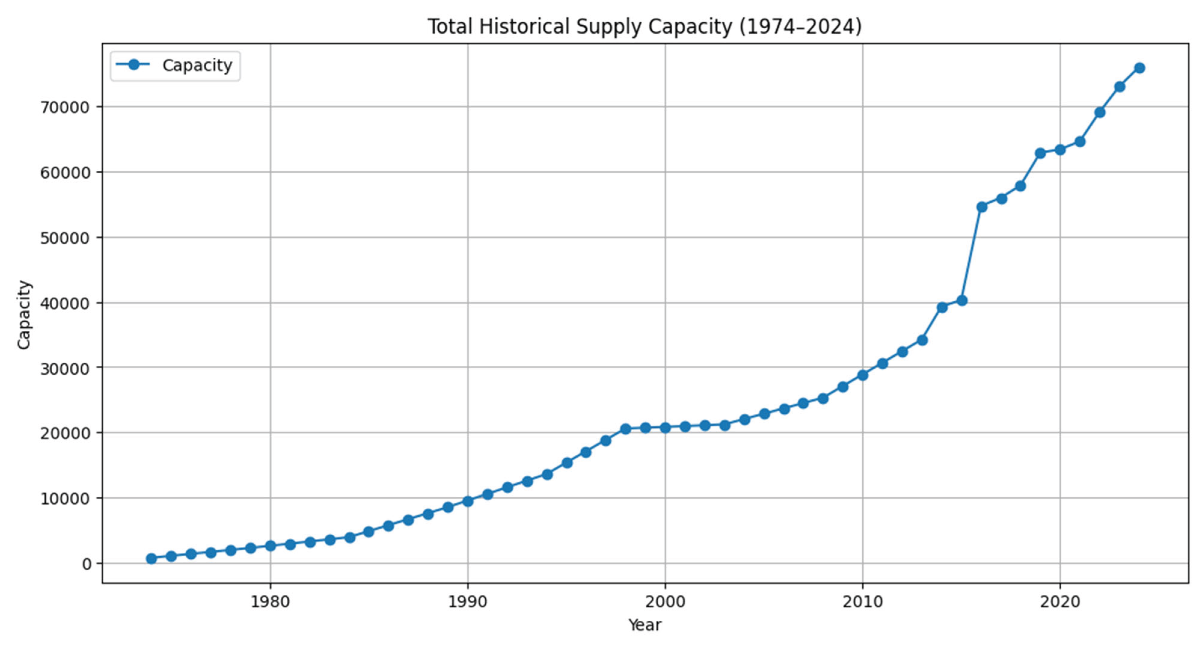
Figure 7.
Indonesia’s Grid Supply 1974-2024.
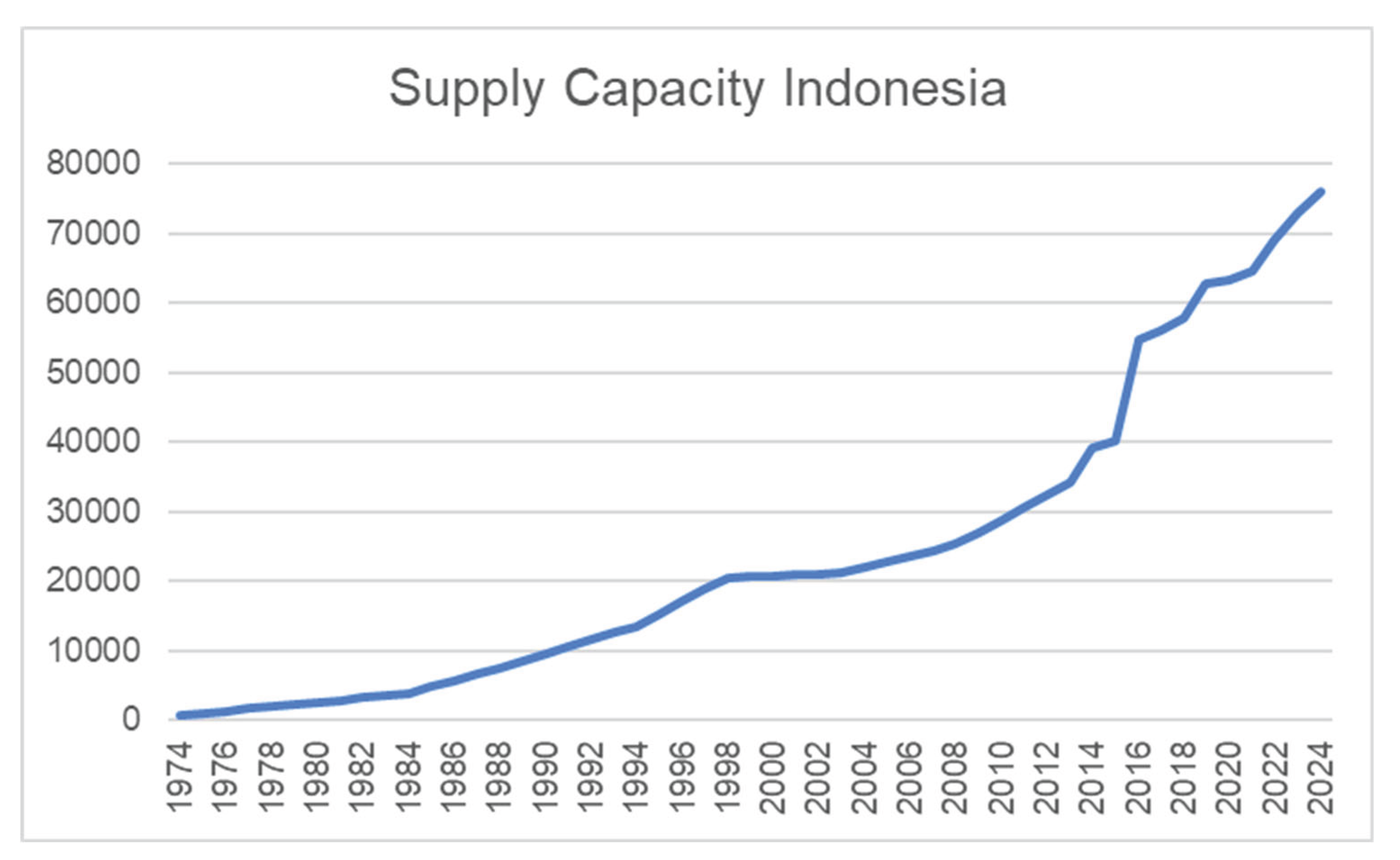
Figure 8.
Grid Supply with 10-year ahead Forecast.
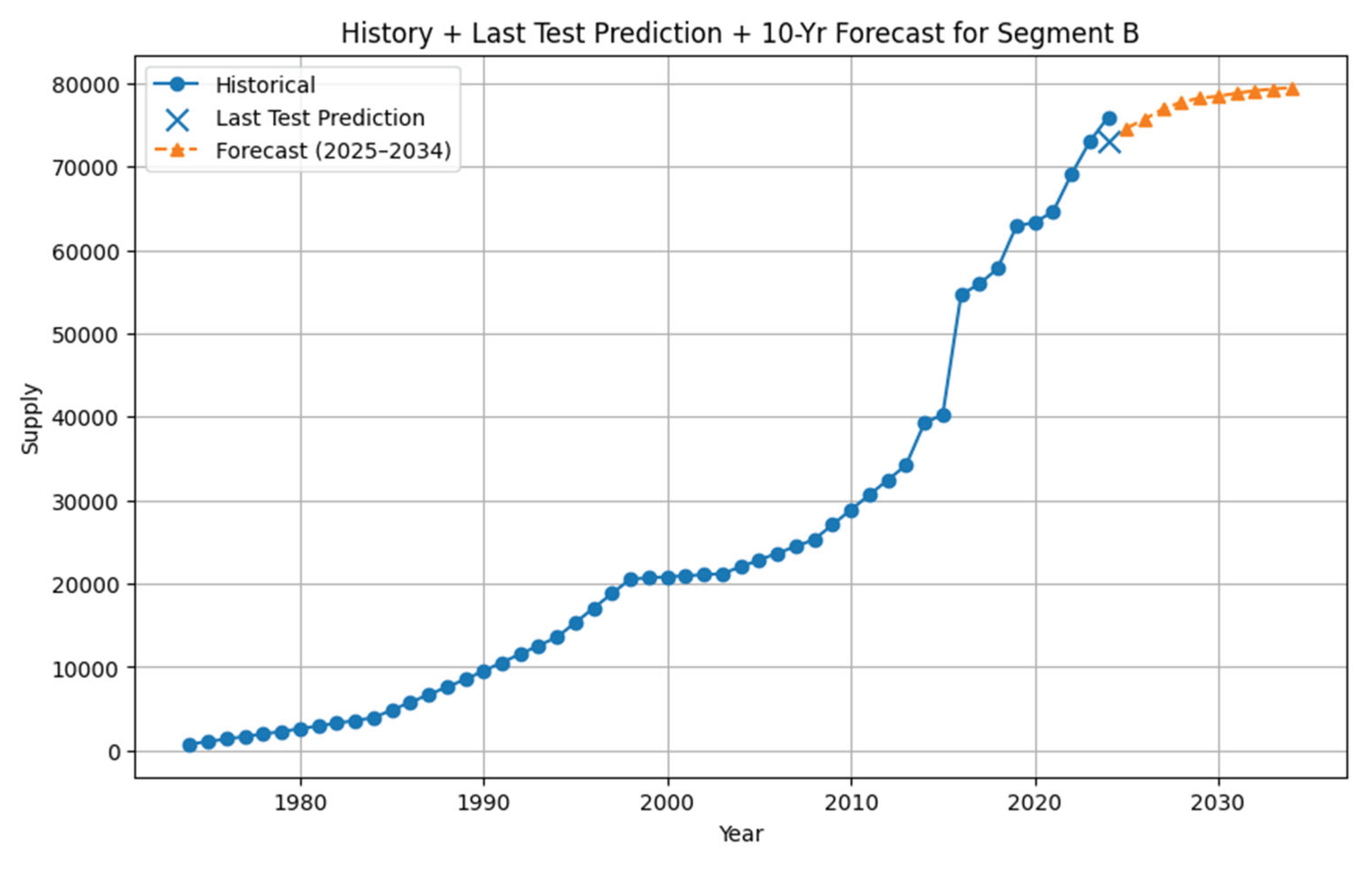
Figure 11.
Initial Annual Growth Rate.
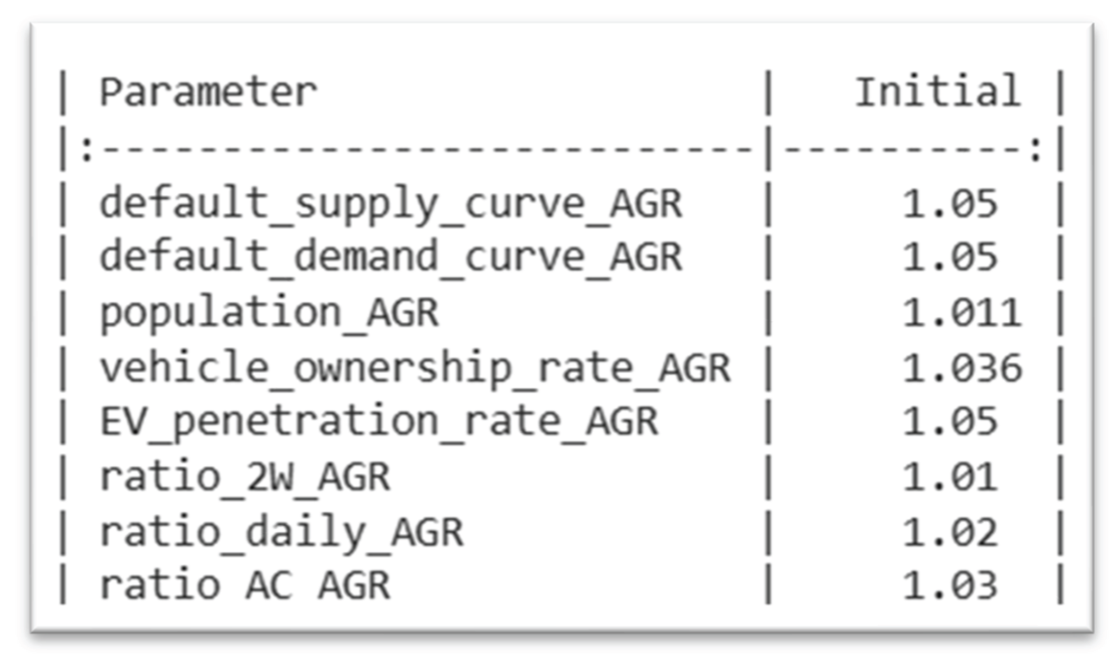
Figure 15.
Weekly ICT Probability.
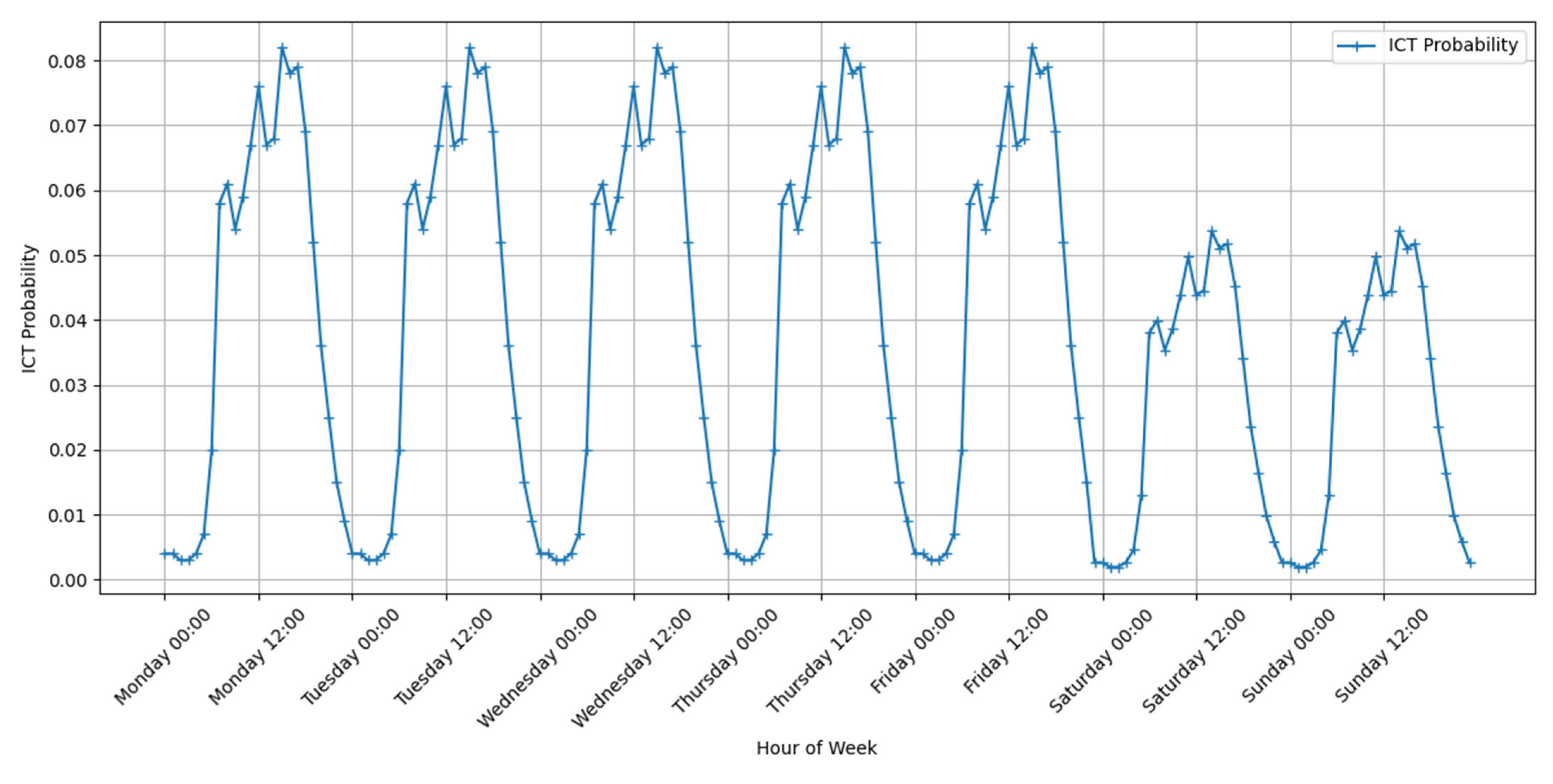
Figure 16.
Vehicle Charge Curve.
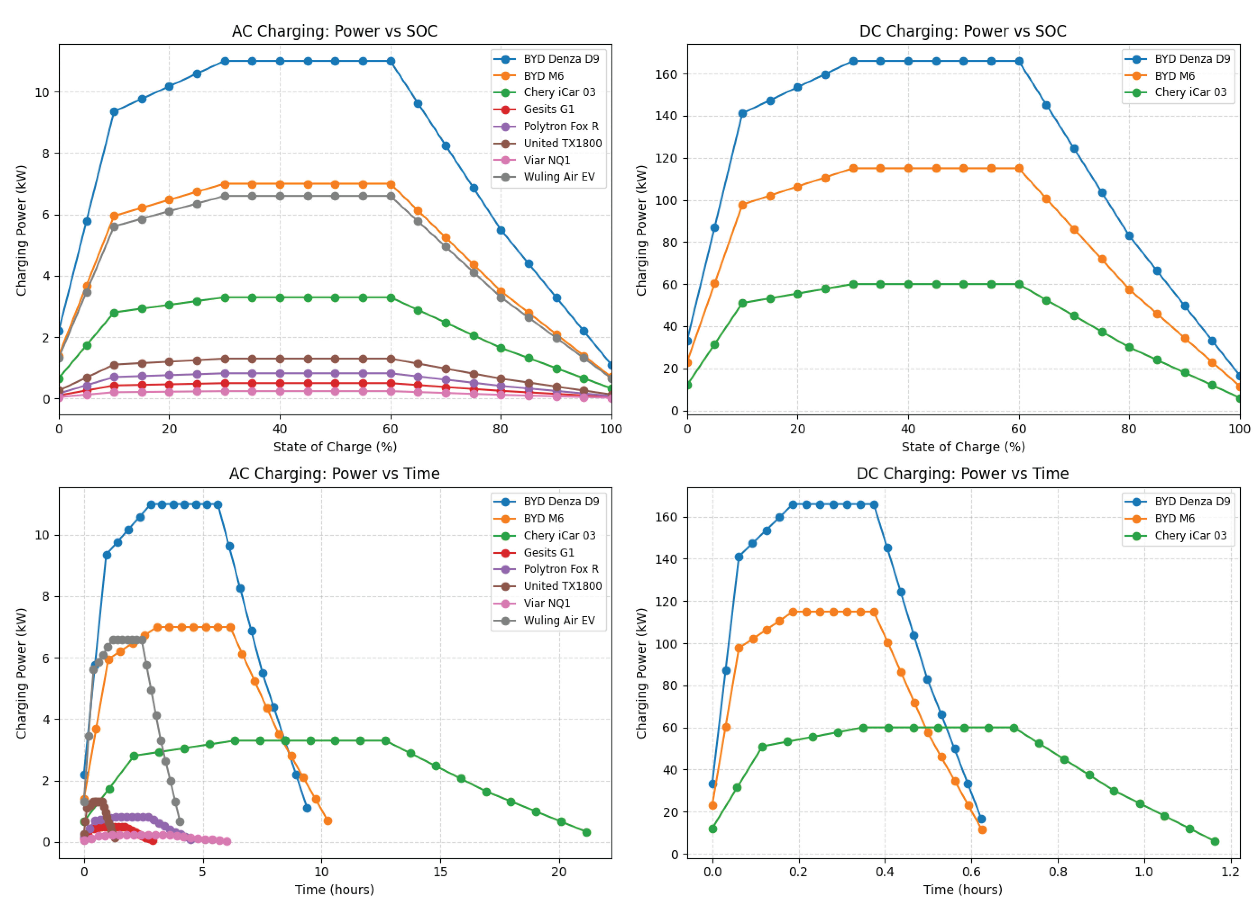
Figure 17.
Calculated EV Population.
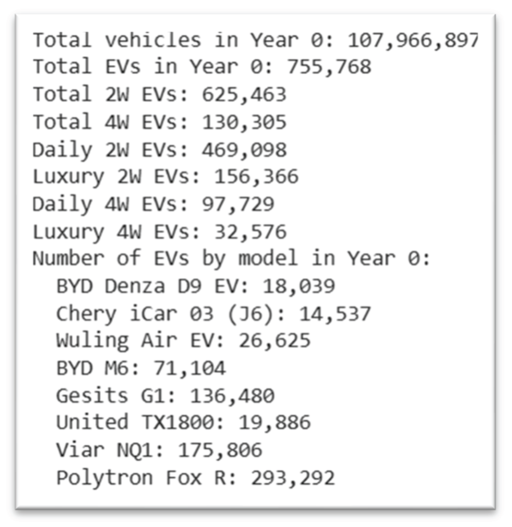
Figure 18.
Charging Load per Vehicle Model.
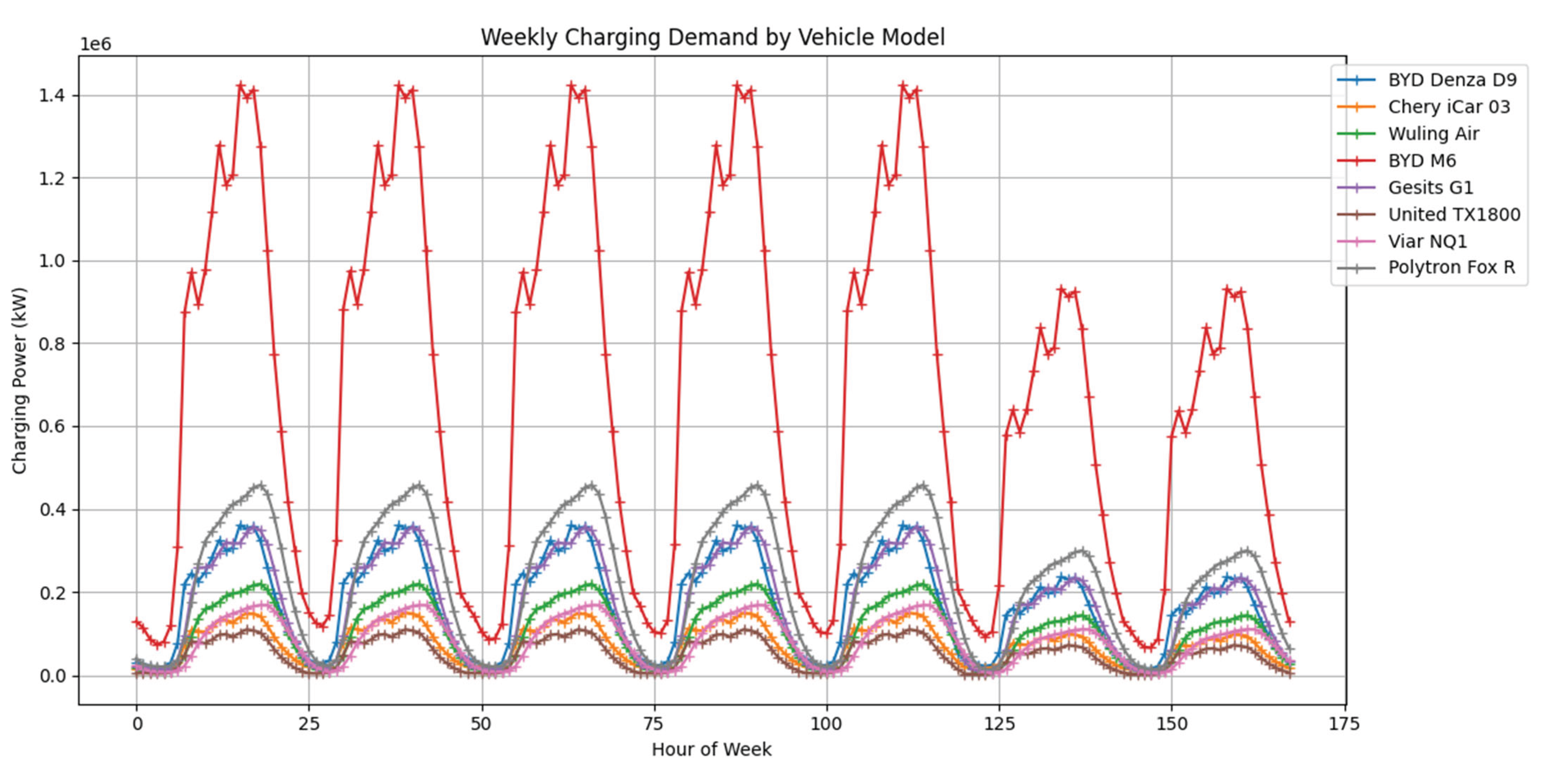
Figure 19.
Charging Load AC and DC.
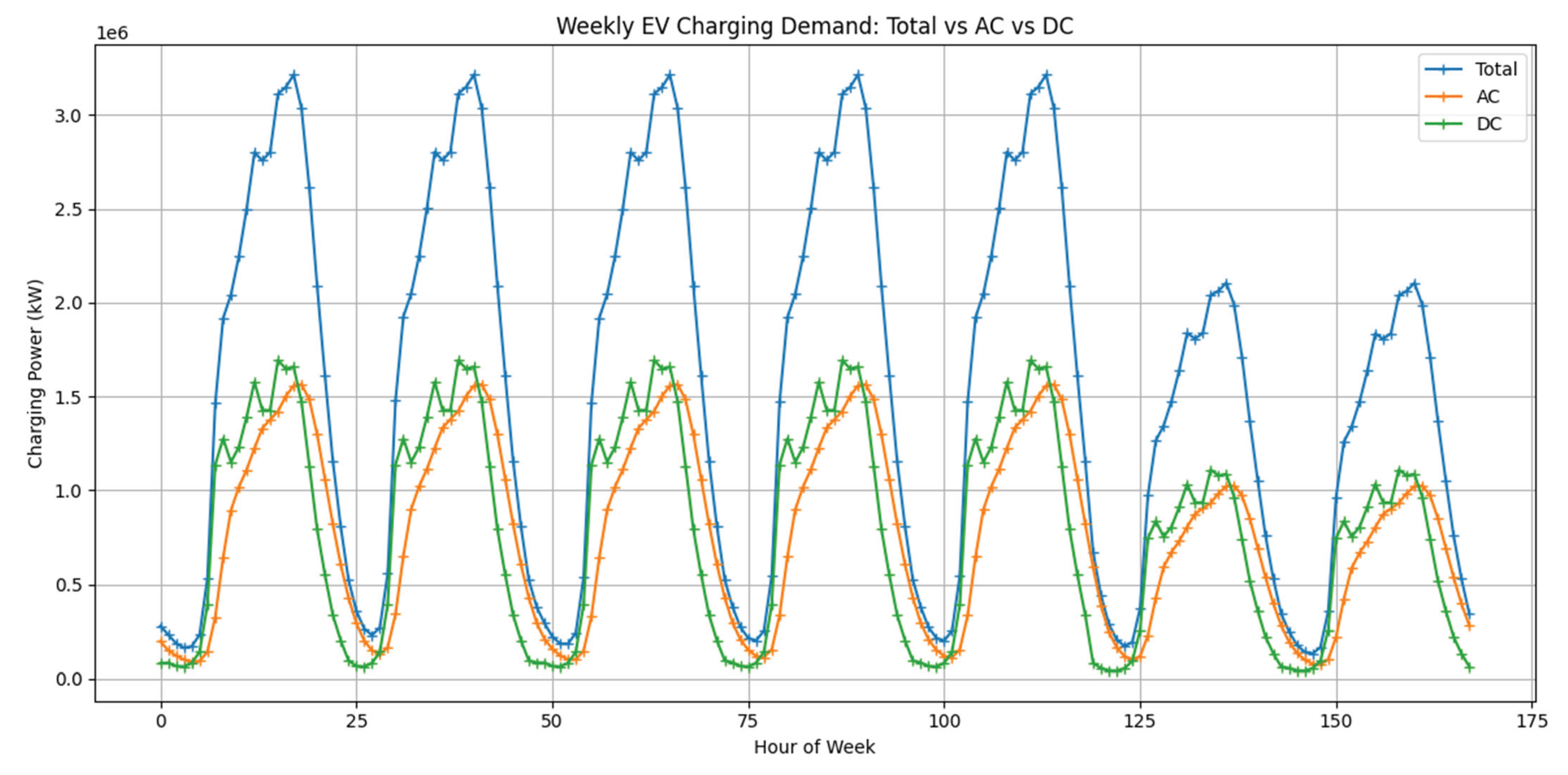
Figure 21.
Supply-Demand Balance Scores.
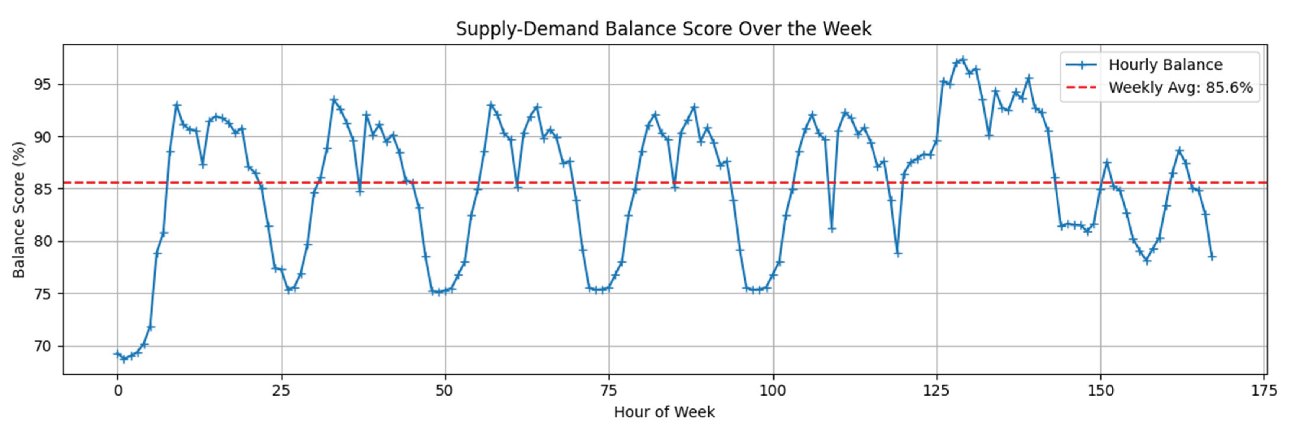
Figure 22.
Total Daily Energy Supply and Demand.
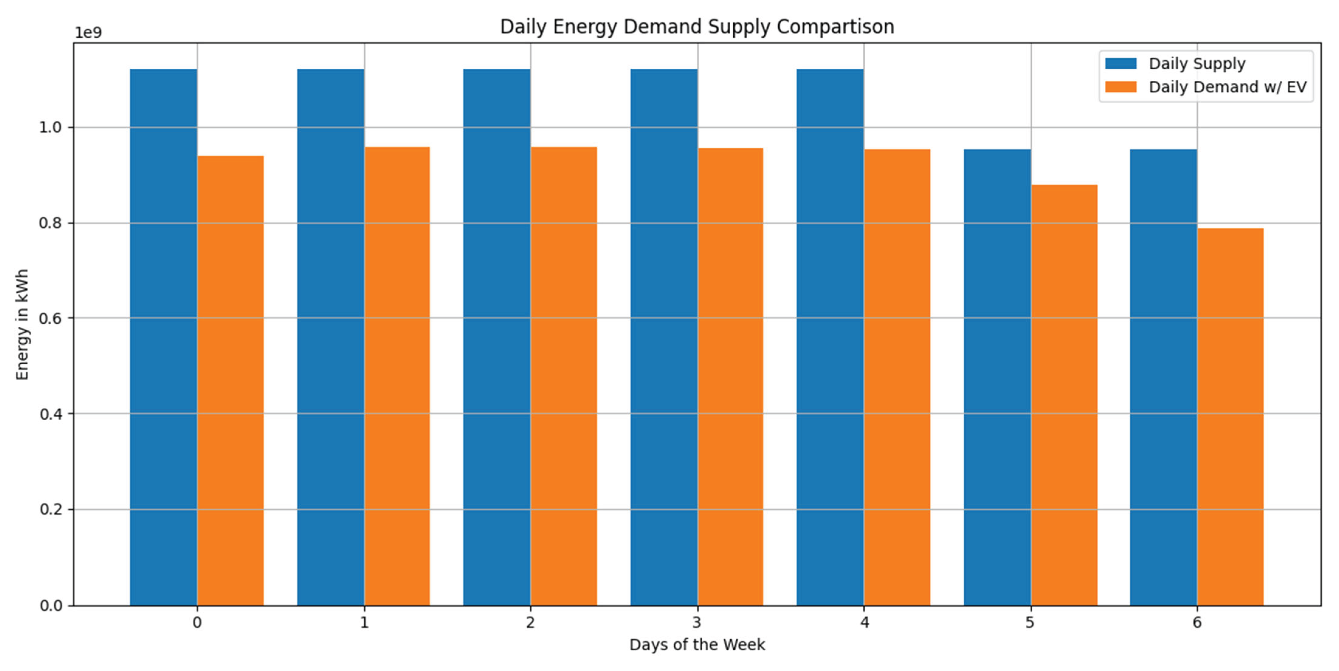
Figure 23.
Weekly Supply and Demand Curves Year0 and Year5.
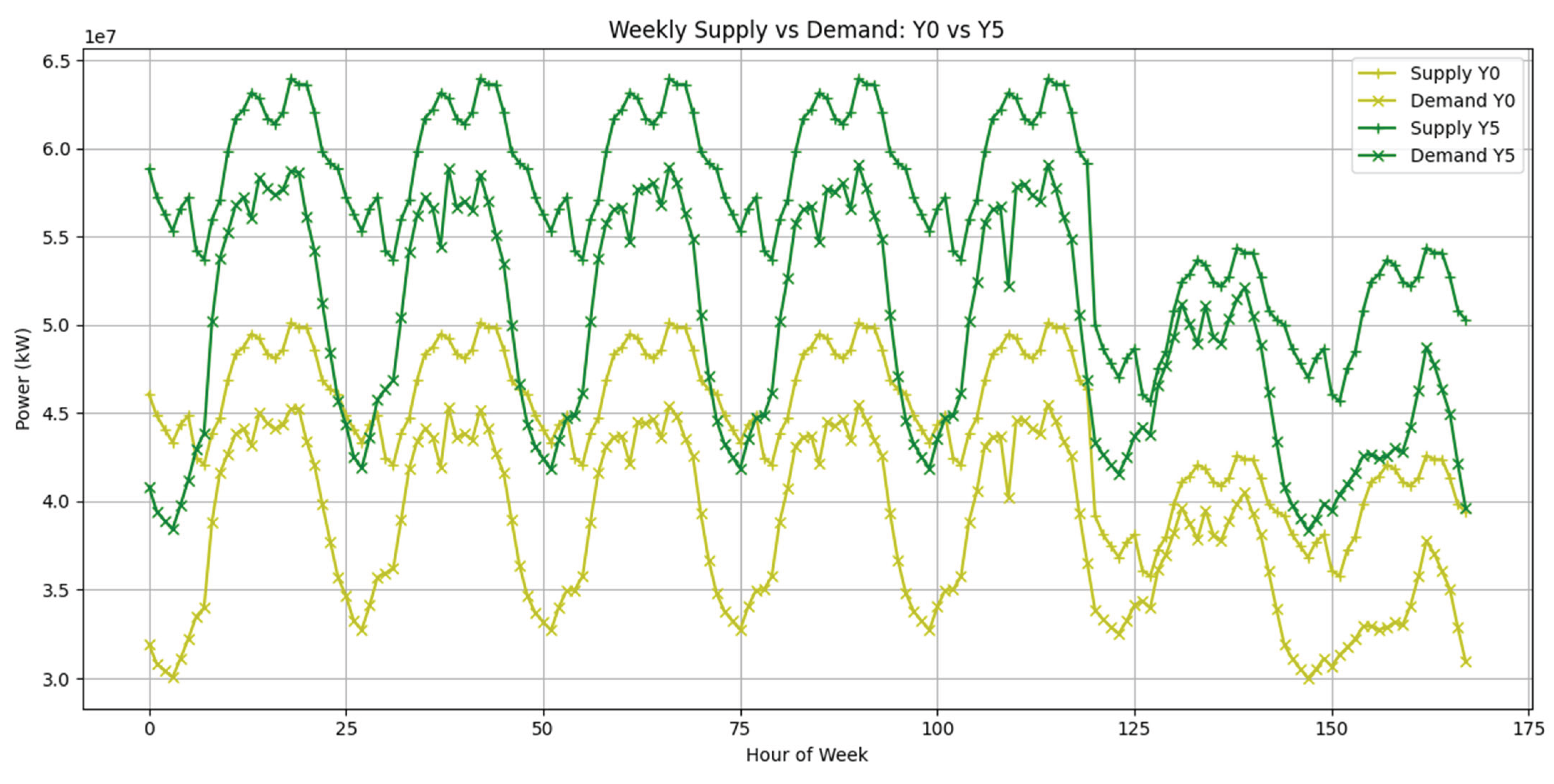
Figure 24.
Total Daily Energy Supply and Demand Year0 and Year5.
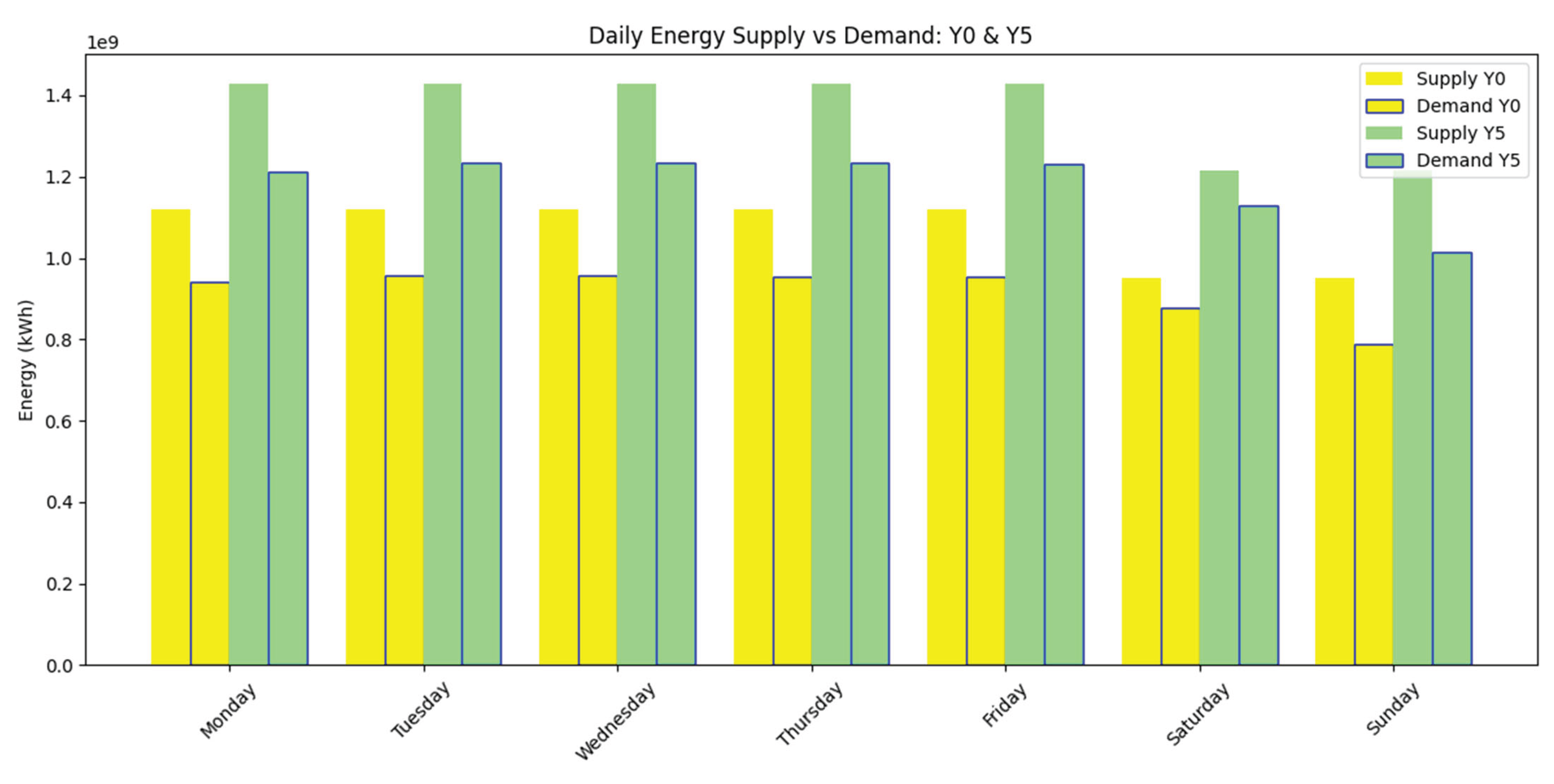
Figure 25.
Annual Average Balance Score.
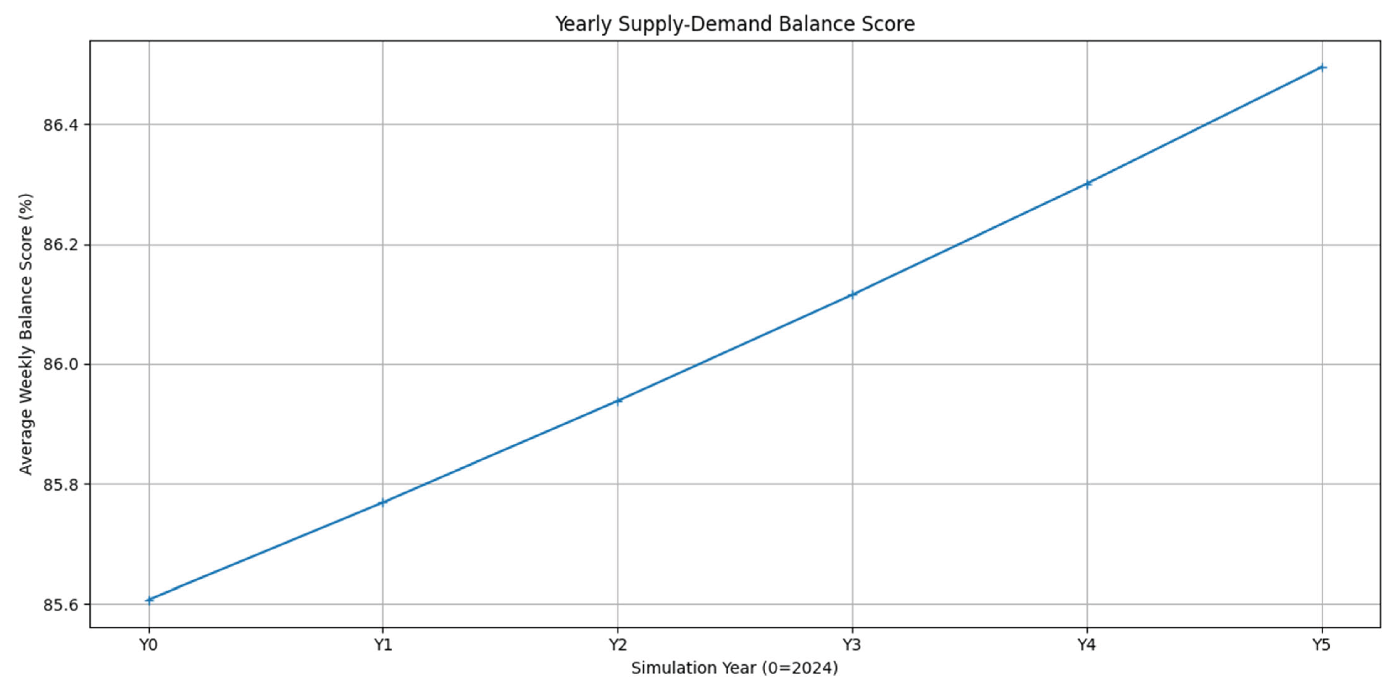
Figure 26.
2026 BAU Supply Demand Curves.
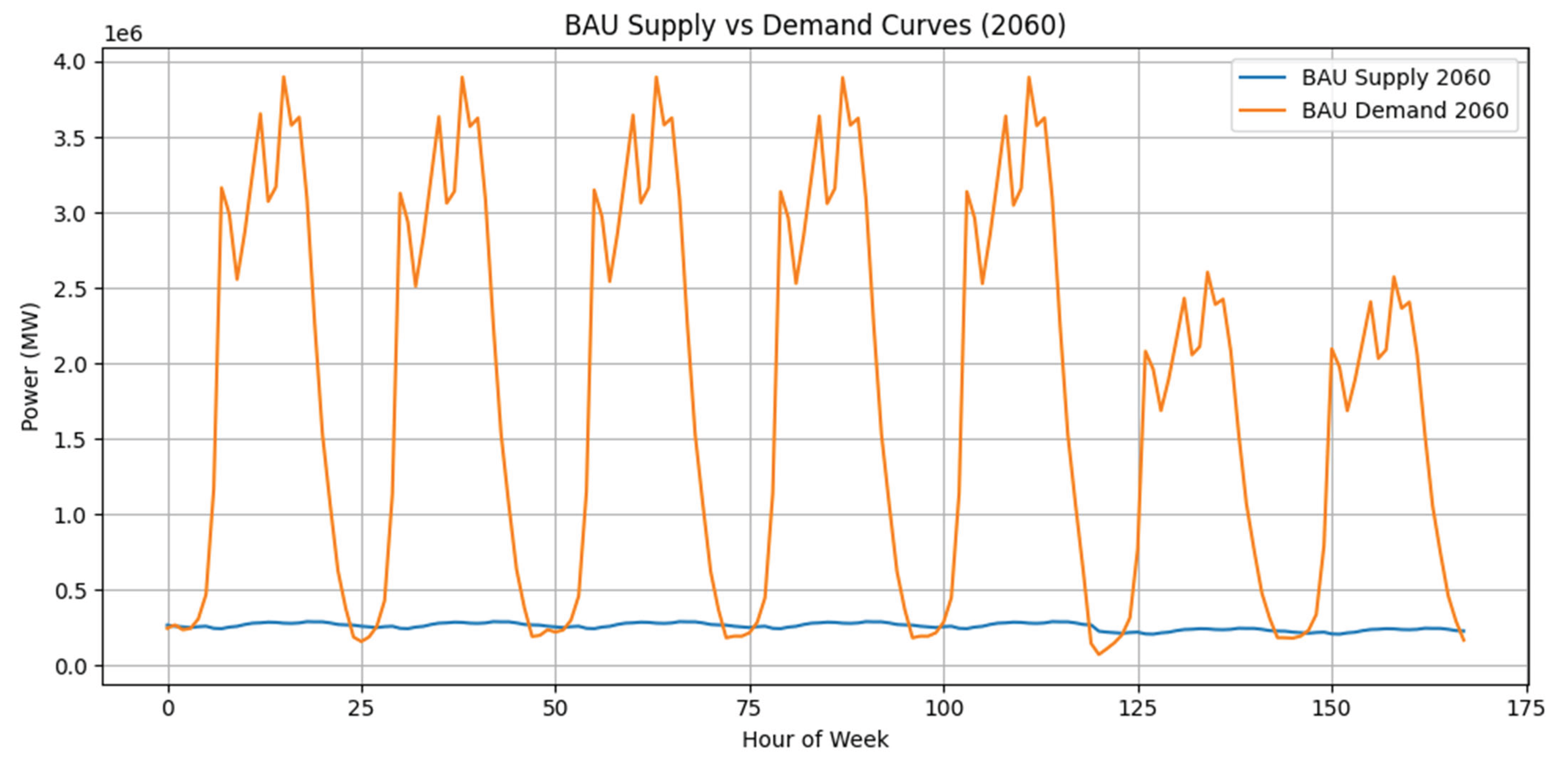
Figure 27.
2026 BAU Daily Supply and Demand.
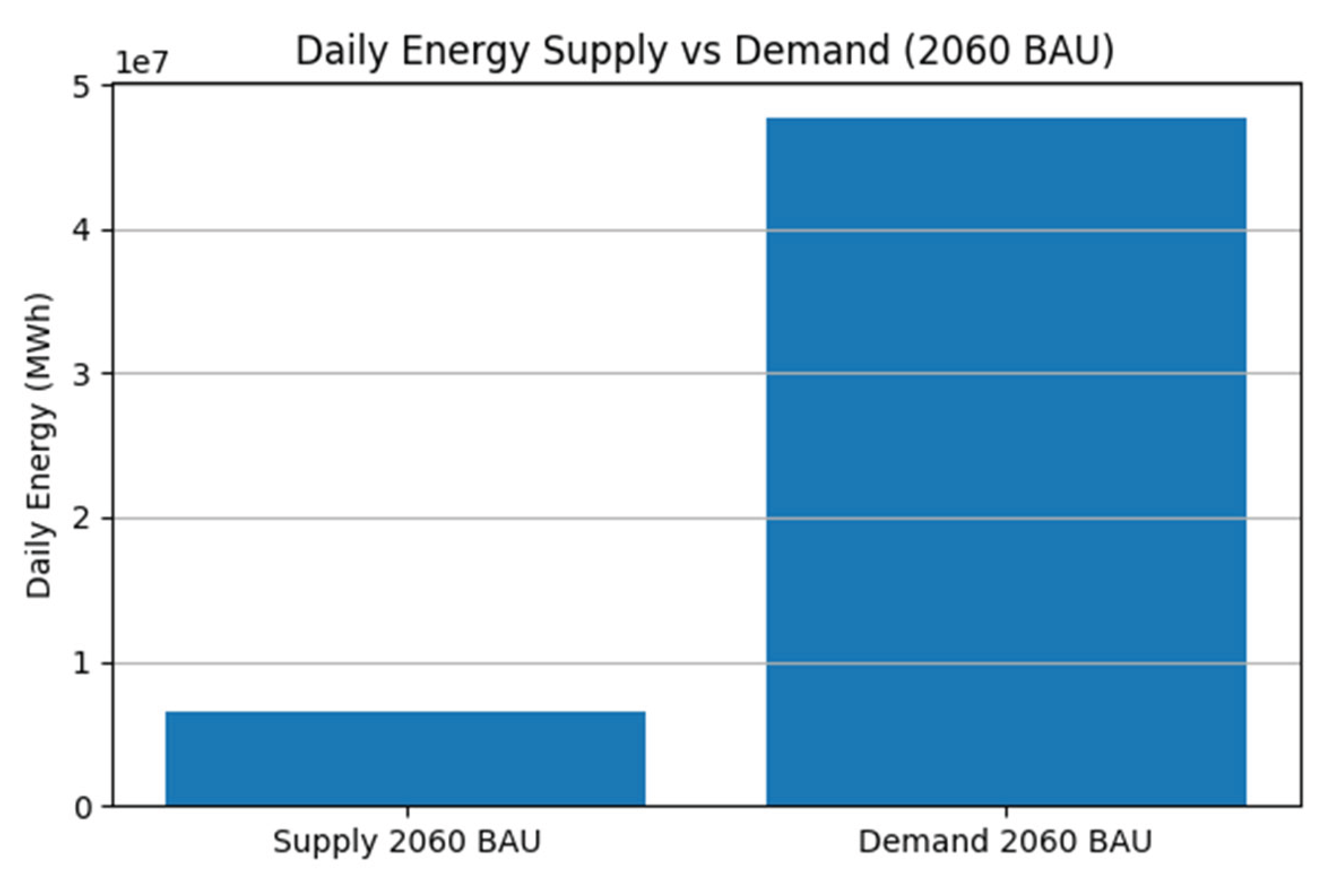
Figure 30.
BAU and Optimized Scenario Balance Score.
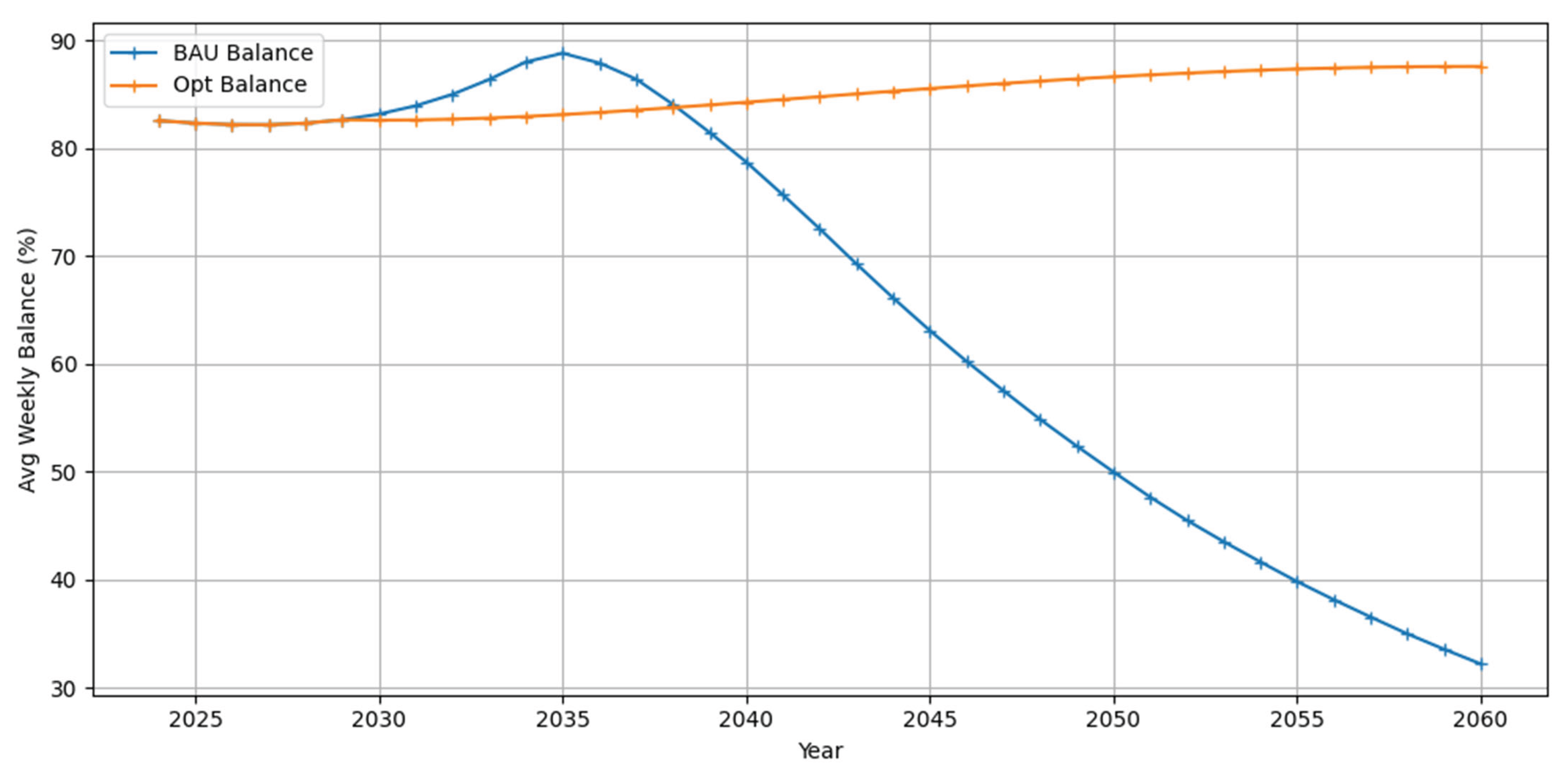
Figure 31.
Daily Energy Gap in MW.
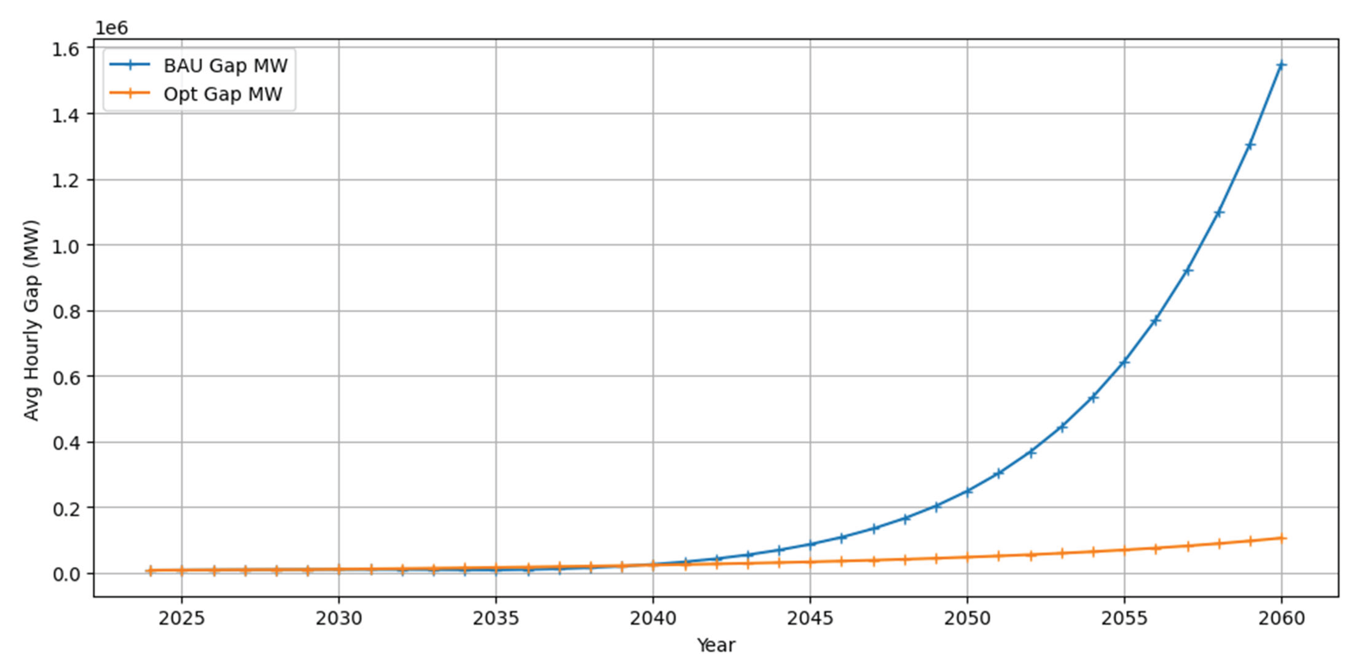
Figure 32.
2026 Supply Demand Curves BAU and Optimized.
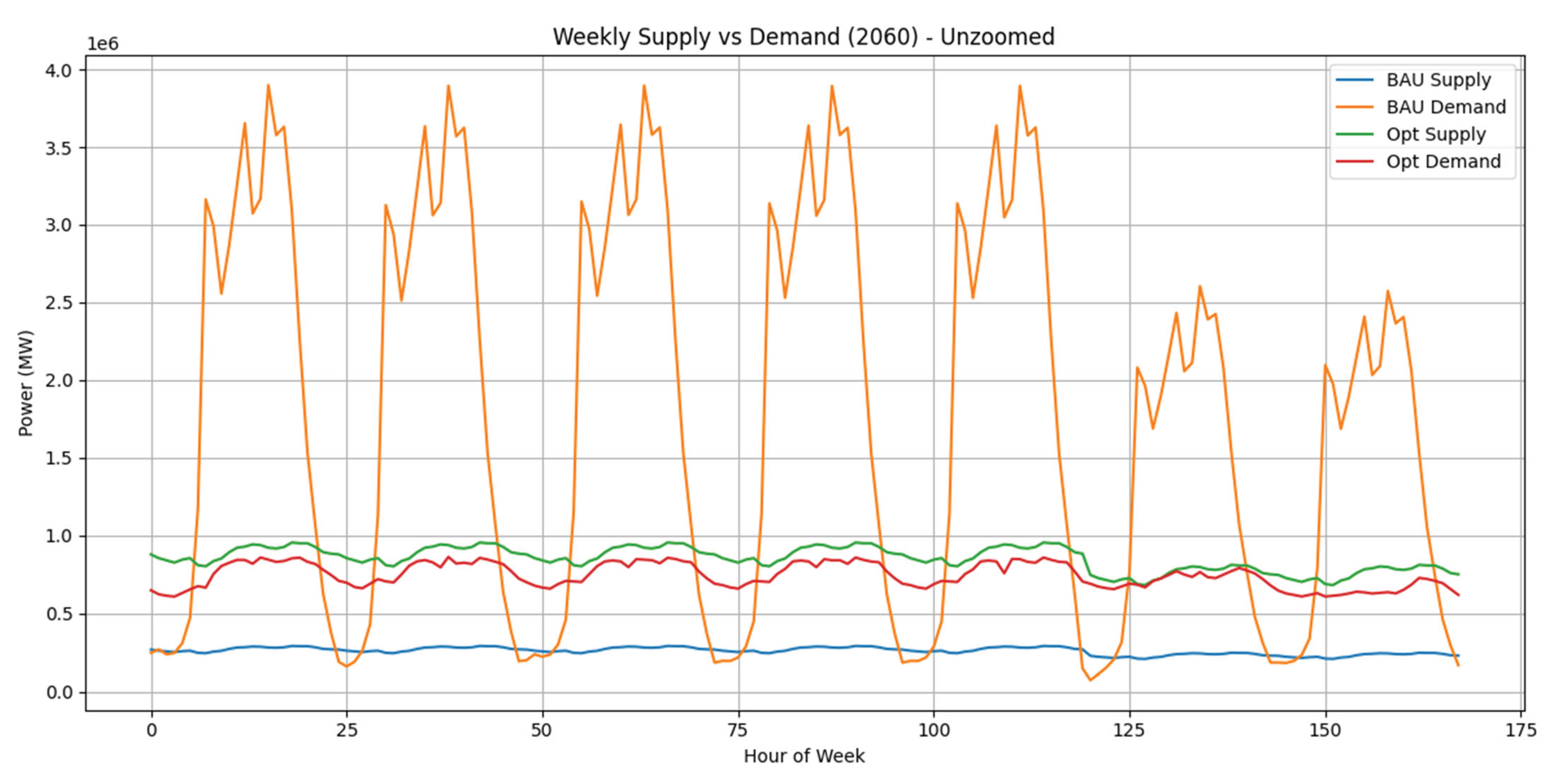
Figure 33.
2026 Supply Demand Curves BAU and Optimized (zoomed).
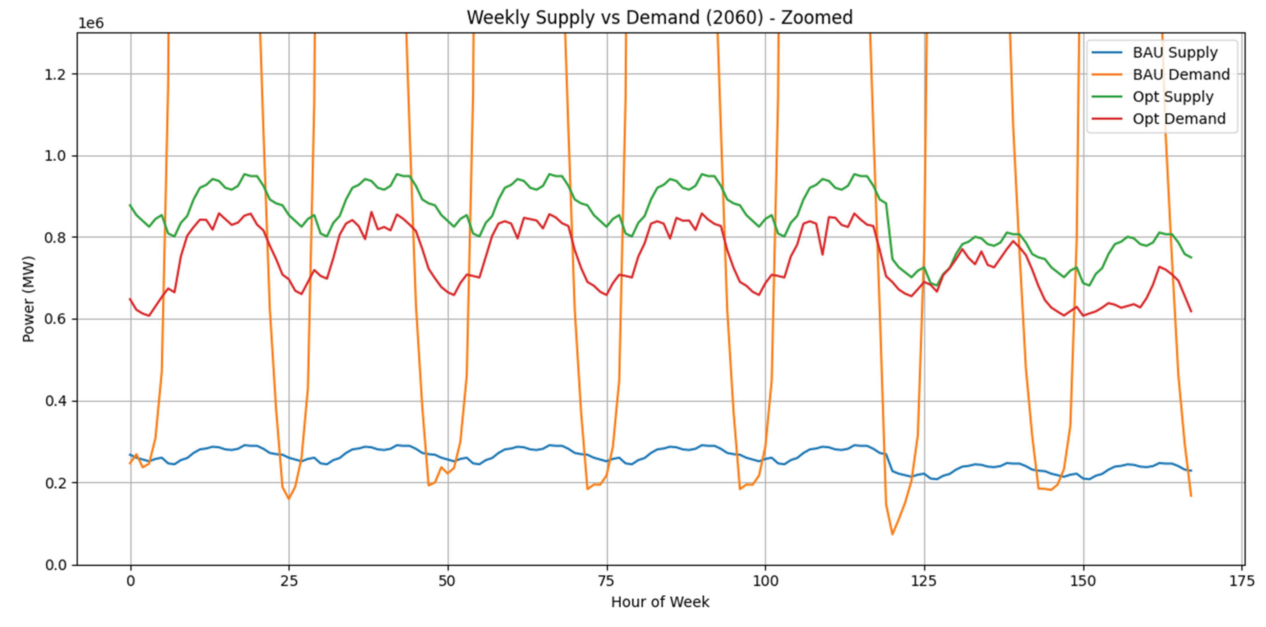
Figure 34.
2026 Daily Energy Supply and Demand BAU and Optimized.
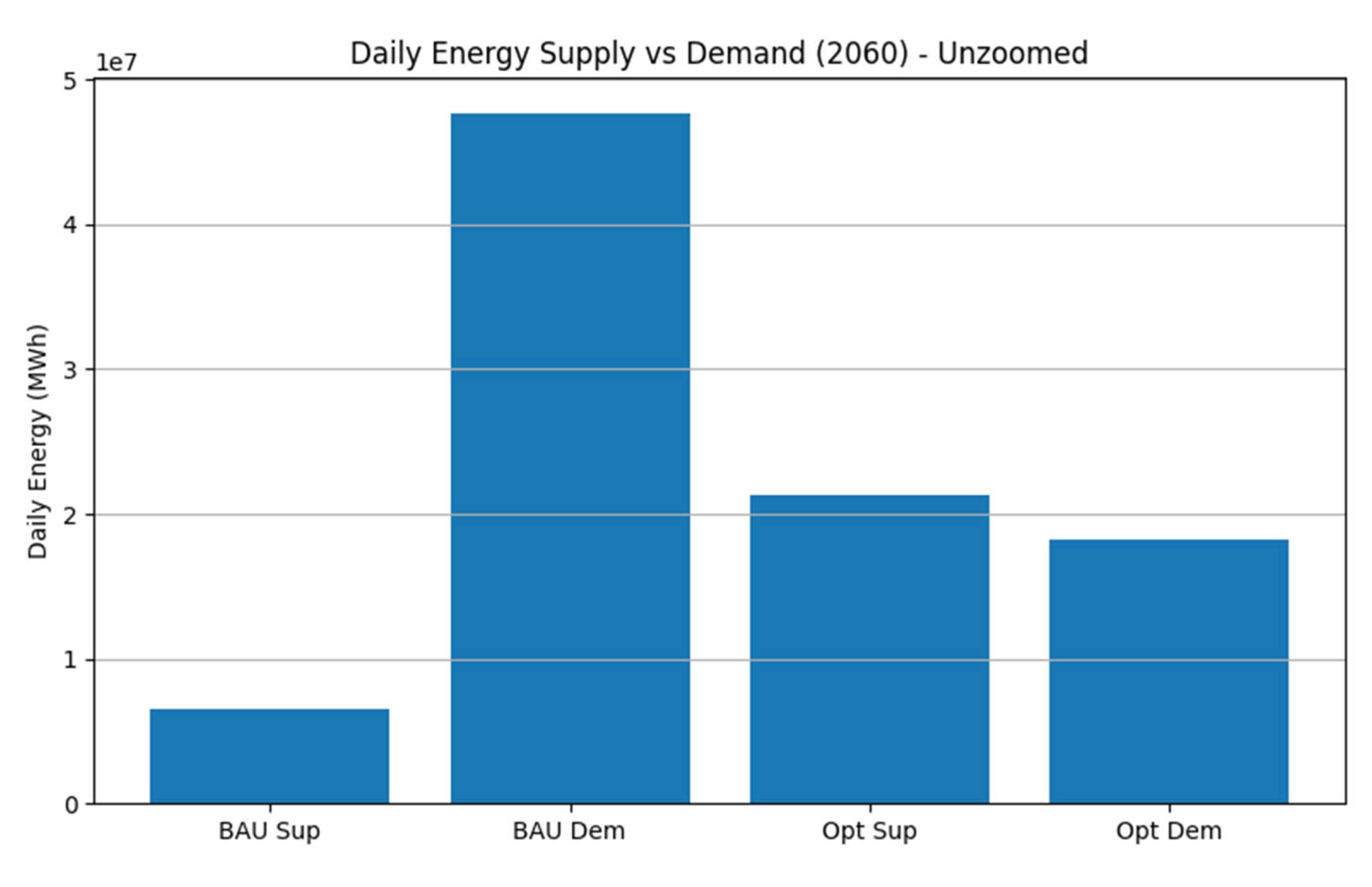
Figure 35.
2026 Daily Energy Supply and Demand BAU and Optimized (zoomed).
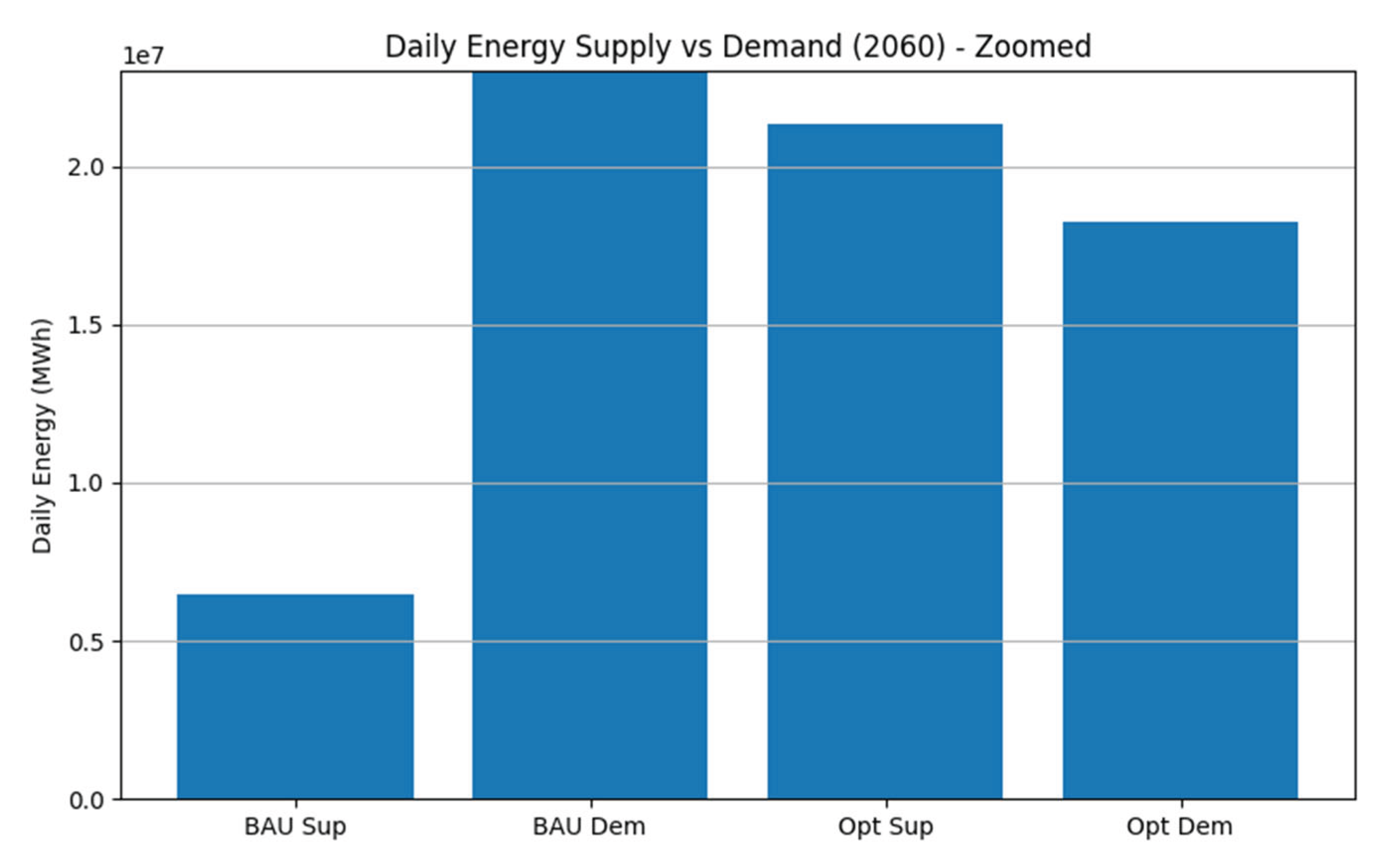
Figure 36.
Annual Cost Saving.
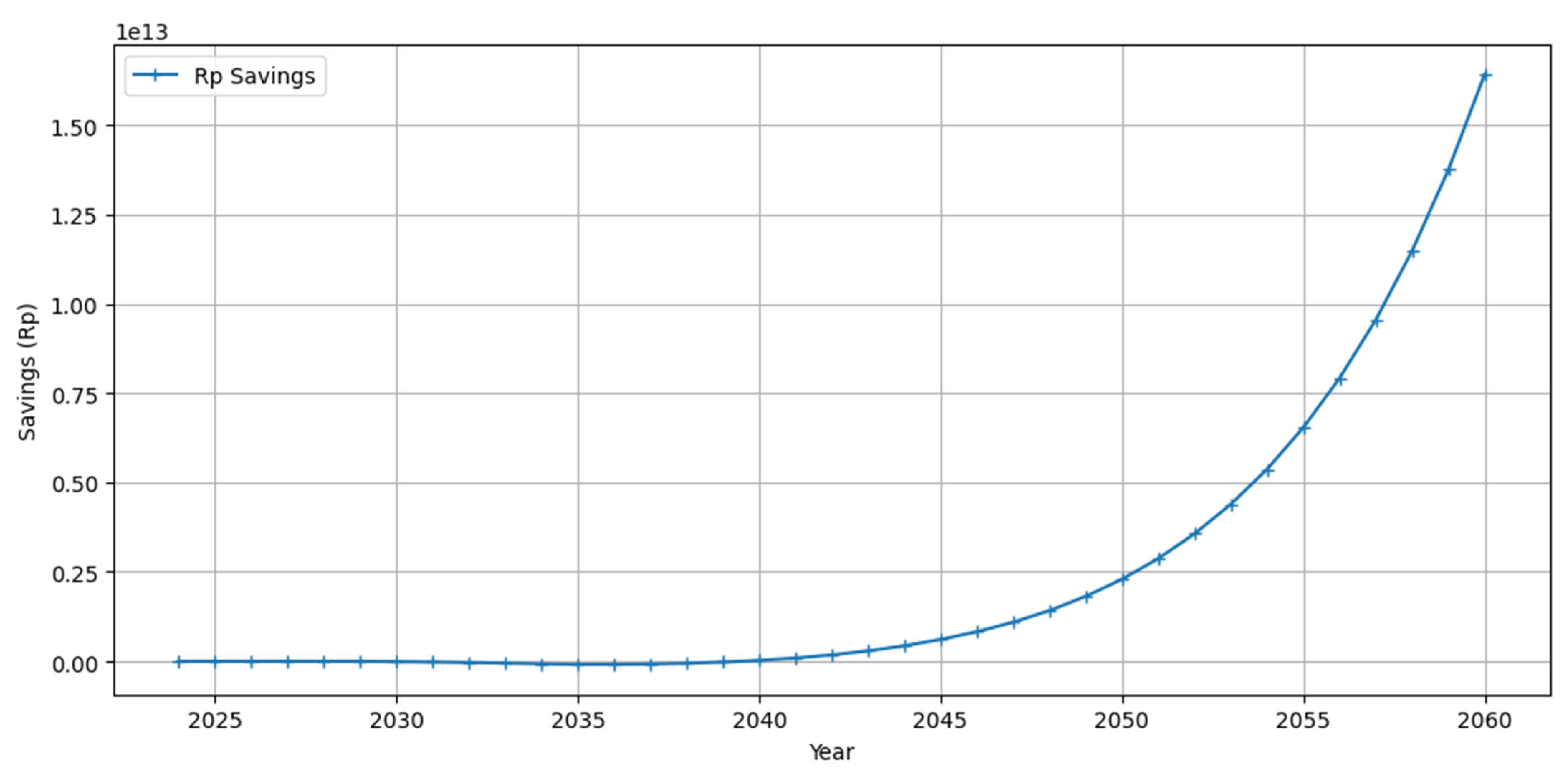
Figure 37.
Annual EV Population BAU and Optimized.
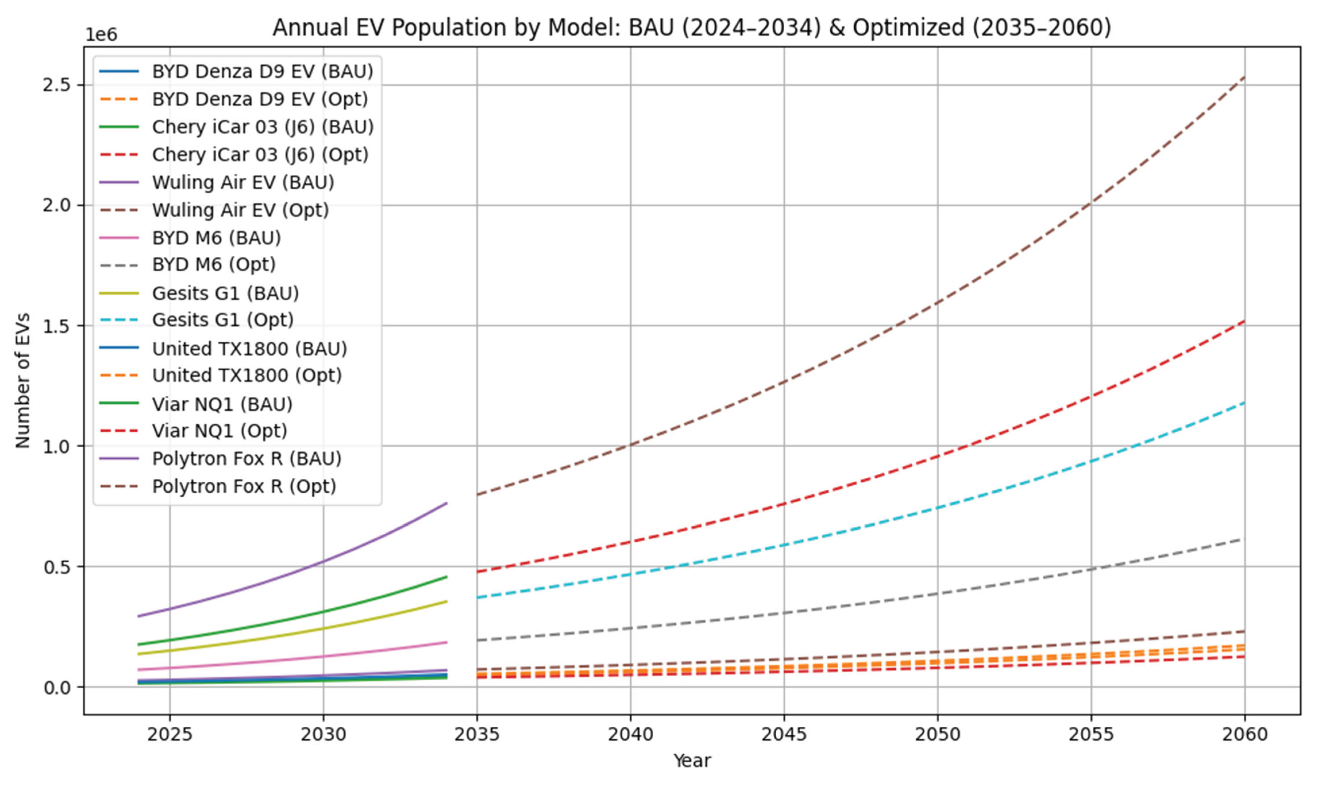
Table 1.
Installed Capacity and Peak Demand Load of Jamali Grid.
| Year | Total Installed Capacity in MW | Peak Demand Load in MW |
| 2014 | 31.062 | 23.908 |
| 2015 | 27.867 | 24.269 |
| 2016 | 36.712 | 33.208 |
| 2017 | 36.517 | 26.580 |
| 2018 | 37.721 | 27.097 |
| 2019 | 40.174 | 26.657 |
| 2020 | 40.685 | 24.420 |
| 2021 | 41.743 | 25.852 |
| 2022 | 45.835 | 24.228 |
| 2023 | 47.647 | 40.223 |
| 2024 | 50.103 | 42.635 |
| Variable Input | Value in Year 0 (2024) |
| Supply Capacity in MW | 50,103 |
| Demand Peak in MW | 42,635 |
| Indonesia Population | 281,603,800 |
| Vehicle Ownership Percentage | 63.9% |
| EV Percentage | 0.7% |
| 2W : 4W Ratio | 4.8 : 5.8 |
| Luxury : Daily Preferences | 25 : 75 |
| Fast : Home Charging Preferences | 25 : 75 |
Disclaimer/Publisher’s Note: The statements, opinions and data contained in all publications are solely those of the individual author(s) and contributor(s) and not of MDPI and/or the editor(s). MDPI and/or the editor(s) disclaim responsibility for any injury to people or property resulting from any ideas, methods, instructions or products referred to in the content. |
© 2025 by the authors. Licensee MDPI, Basel, Switzerland. This article is an open access article distributed under the terms and conditions of the Creative Commons Attribution (CC BY) license (http://creativecommons.org/licenses/by/4.0/).
Copyright: This open access article is published under a Creative Commons CC BY 4.0 license, which permit the free download, distribution, and reuse, provided that the author and preprint are cited in any reuse.


