Submitted:
22 May 2025
Posted:
23 May 2025
You are already at the latest version
Abstract
Accurate forecasting is essential for effective energy management, particularly in evolving and data-driven energy markets. This study presents a hybrid multi-stage forecasting framework to enhance short- and long-term electricity demand predictions in the Netherlands. We compare statistical (SARIMAX), hybrid (SARIMAX-LSTM), and deep learning (sequence-to-sequence) models across forecasting horizons ranging from 1 to 180 days. The models were trained on daily load data from ENTSO-E (2009-2023) and enriched with external variables, including weather conditions, energy prices, socioeconomic indicators, and engineered features such as calendar effects and rolling demand windows. Three feature configurations were evaluated: exogenous-only, generated-only, and a combined set. Internally generated features consistently outperformed exogenous inputs, particularly in long-term forecasts. The sequence-to-sequence model achieved the highest accuracy at the 180-day horizon, with a mean absolute percentage error (MAPE) of approximately 1.88%, outperforming both SARIMAX and the SARIMAX-LSTM hybrid. An additional SARIMAX-based analysis assesses the individual effects of renewable and socioeconomic indicators. Renewable energy production data improve short-term accuracy (MAPE reduced from 2.13% to 1.09%), but contribute little to long-term predictions. Socioeconomic variables slightly degrade predictive performance.
Keywords:
energy demand
; time series
; renewable energy
; machine learning
; long short-term memory
; SARIMAX
; sequence-to-sequence
1. Introduction
Electricity is the backbone of modern economies, driving industries, businesses, and households alike. It powers essential infrastructure, fuels technological advancements, and plays a pivotal role in the global transition toward sustainable energy systems [1,2]. Globally, and locally, electricity demand is steadily rising, influenced by economic growth, increased electrification in transport and heating, and the expansion of energy-intensive industries such as data centers [3,4]. However, as the country moves away from coal and natural gas in favor of weather-dependent renewables, maintaining a stable electricity supply has become a significant challenge [5]. According to the Netherlands’ National Energy System Plan, electricity supply is expected to increase fourfold by 2050. Achieving this target will require a significant scale-up of renewable energy deployment, leveraging the country’s established strengths in solar PV and wind energy [6]. Grid operators like TenneT warn that energy shortages could emerge in regions such as Noord-Holland as early as 2026 [7]. Consequently, accurate electricity demand forecasting is critical for energy system stability, efficient resource allocation, and policy planning [8].
Energy demand forecasting serves multiple purposes. Accurate predictions optimize energy distribution, reducing operational costs and preventing supply-demand imbalances [9,10]. Underestimating demand can lead to power shortages, disruptions in economic activity, and grid instability, whereas overestimating demand can result in unnecessary investments and financial inefficiencies. With global electricity demand expected to increase at an average annual rate of 4% through 2027 [3], improving forecasting techniques is essential for ensuring a reliable, cost-effective, and sustainable energy transition.
Electricity consumption is shaped by a complex interplay of factors [11]. While historical consumption patterns provide a baseline for prediction, external variables introduce fluctuations that complicate forecasting. Weather and climate conditions, such as temperature, humidity, and wind speed, directly impact heating, cooling, and overall electricity usage. Socioeconomic trends, including population growth and economic activity, shape long-term demand patterns, while the transition to renewable energy introduces new uncertainties due to the variability of wind and solar generation [12]. Additionally, fluctuations in energy prices play a crucial role in shaping consumer behavior, particularly among low-income households. In 2020, for instance, energy consumption reached its lowest point, largely due to rising costs, underscoring the strong relationship between price increases and reduced demand [13].
Classical statistical models, such as time series approaches, often outperform AI-based models in long-term forecasting, particularly when trends and seasonality remain stable. These models provide strong interpretability and consistency over time [14]. However, AI models, especially deep learning techniques like LSTM, and sequence to sequence excel in capturing complex, non-linear relationships, making them highly accurate for short-term forecasts [14,15]. Despite their advantages, AI-based models struggle with long-term dependencies due to issues such as vanishing gradients, and are heavily reliant on data quality, computational resources, and careful tuning [16,17]. This reliance can obscure variable relationships and complicate model interpretation. To effectively forecast energy demand while addressing both long-term trends and short-term fluctuations, a hybrid modeling approach is recommended.
This paper presents a novel approach to forecasting national electricity demand in the Netherlands by evaluating and comparing classical statistical, hybrid, and deep learning models. The baseline model, SARIMAX, is selected due to its widespread use in energy forecasting and its well-documented ability to model seasonality, trends, and autocorrelation with transparency [18,19]. Its interpretability and robustness make it a strong reference point for evaluating the added value of more complex models. To improve onhis benchmark, two alternative models are proposed: a hybrid SARIMAX–LSTM model that combines linear and nonlinear forecasting capabilities, and a deep learning-based sequence-to-sequence (seq2seq) model designed to capture complex temporal dependencies. By incorporating key external predictors, such as climate variability, energy prices, and socioeconomic indicators, together with engineered temporal features, each model is evaluated for its ability to capture short-term fluctuations and long-term trends. Unlike previous studies focused on small-scale or regional forecasting, this work applies these methods at the national level and investigates the role of energy source composition and socioeconomic factors in shaping forecast accuracy.
This study aims to evaluate how the integration of heterogeneous feature sets influences the performance of statistical, hybrid, and deep learning models in forecasting electricity demand across short and long-term horizons. Specifically, we examine the added predictive value of renewable energy production data and assess the role of socioeconomic indicators such as GDP and population. Three models are compared, SARIMAX, a hybrid SARIMAX-LSTM model, and a sequence-to-sequence deep learning model, across different feature configurations to determine their effectiveness in capturing temporal dynamics and improving forecast accuracy at the national level.
2. Related Work
Energy demand forecasting is a critical area of research, especially as global energy systems face increasing complexities due to climate targets and shifts toward renewable sources [20]. Since the 1950s, a wide range of methodologies has emerged to address the intricate patterns of energy consumption, from traditional statistical models to advanced machine learning and hybrid techniques. Despite these advancements, a key research gap remains: few models adequately capture the effects of rising green energy adoption on natural gas demand and electricity[14]. This study seeks to fill this gap by developing adaptable forecasting models that respond to the dynamics of energy transitions.
2.1. Influencing Factors in Energy Load Forecasting
2.1.1. Socioeconomically Factors
Gross Domestic Product (GDP) strongly influences energy demand [14,21]. Economic growth drives industrial production, commercial services, and household consumption, increasing energy use. Industrialized economies rely on energy-intensive manufacturing, while service-based economies require substantial energy for infrastructure. In developed nations, efficiency improvements and renewables have reduced the link between GDP and energy use, whereas developing countries still see rising demand due to urbanization and industrial expansion. In the Netherlands, GDP grew by 0.9% in 2024 [22].
Population growth is a key driver of rising energy demand, as expanding populations lead to greater residential energy consumption for housing, appliances, and transportation [8,14]. This effect is further intensified by urbanization, which fuels energy demand in commercial buildings, public transport, and infrastructure. In the Netherlands, the population has grown rapidly, reaching approximately 18 million in 2024—an increase of about 1.1 million over the past decade. This growth is largely driven by high life expectancy, economic expansion, and job opportunities. Major cities such as Amsterdam, Rotterdam, and The Hague continue to see rising demand, with Amsterdam alone home to nearly 800,000 residents. [23].
Energy prices have a significant impact on energy demand, influencing both consumer behavior and industrial operations. In 2022, rising energy costs, driven by inflation, led to a noticeable decline in energy consumption as households and businesses sought to reduce expenses through energy-saving measures. In response, the Dutch government has introduced additional policies to cushion the effects of inflation and surging energy prices, particularly for low- and middle-income households. Inflation is expected to rise further, potentially reaching 5.2% this year, primarily due to increased energy costs. Consequently, average purchasing power is projected to decline by 2.7% [24].
Together, GDP, population, and energy prices form a complex relationship that drives energy consumption trends. While economic growth and population expansion generally lead to higher energy demand, energy prices act as a balancing factor, influencing how individuals and businesses respond to changes in supply and affordability. The interplay of these factors, alongside technological advancements and sustainability policies, determines the long-term trajectory of energy demand across different regions and economies. Although GDP and population data are available only at a yearly resolution, they provide valuable structural context for long-term energy consumption patterns. In larger daily forecasting horizons, where short-term seasonality becomes less dominant, incorporating such stable indicators helps capture the broader socioeconomic trends that influence aggregate demand levels [25].
2.1.2. Weather & Renewable Energy
Weather variables such as temperature, humidity, and wind speed significantly influence energy demand patterns by affecting heating and cooling requirements. For instance, a study conducted in the Netherlands shows that energy demand peaks during colder months due to increased heating needs [26]. Similarly, research in Prague has demonstrated that warmer weather reduces heating demand while simultaneously increasing the need for cooling infrastructure [27].
In parallel, renewable energy sources, especially solar and wind, have become critical components of modern energy systems. Their outputs are inherently weather dependent, introducing new levels of variability into the grid. The Netherlands aims to deploy more renewables in order to quadruple its electricity supply [6]. Therefore, integrating weather and renewable energy variables into prediction models is essential. These features not only capture the direct influence of environmental conditions on consumption patterns but also reflect fluctuations in supply due to the intermittent nature of renewables. This dual impact makes them key predictors in short-term forecasting models [4].
2.2. Classical Statistical Models for Long-Term Forecasting
Classical statistical models, particularly time series (TS) methods, have long been effective in long-term forecasting scenarios, especially where seasonal patterns and trends remain relatively stable [14,28]. These models leverage historical data to identify patterns and generate forecasts, making them valuable tools for understanding the influence of past trends on future outcomes. A widely used model, like ARIMA, is known for its strong interpretability and robustness in low-volatility environments. It has been commonly applied to forecast total gas demand as well as specific subsectors like households and industries, often utilizing confidence intervals to assess the reliability of predictions [29,30]. Variants of ARIMA, such as seasonal ARIMA (SARIMA), incorporate seasonal and external factors, further enhancing their predictive capabilities for energy demand forecasting [14]. Research indicates that these models frequently outperform AI techniques in long-term forecasts due to their reliance on well-established patterns rather than extensive datasets. However, they exhibit notable limitations when faced with complex, non-linear relationships or significant short-term demand fluctuations, where more adaptive and data-driven approaches may be required [8].
2.3. Applications of Machine Learning and Deep Learning in Energy Forecasting
AI-based forecasting techniques, encompassing both machine learning and deep learning, have become essential tools for improving the accuracy and adaptability of energy demand predictions. These methods excel at capturing complex and nonlinear relationships, which are challenging for traditional statistical models.
ML methods, such as Support Vector Regression (SVR) and Stochastic Gradient Descent (SGD), have demonstrated strong potential in short-term forecasting tasks [31,32]. SVR, leveraging linear and Radial Basis Function (RBF) kernels, effectively captures both linear and nonlinear data patterns. Meanwhile, SGD optimizes gradient descent by using random subsets, offering computational efficiency and fast convergence, particularly in large-scale scenarios. Among these models, SGD has achieved the highest prediction accuracy, showcasing its scalability and precision in forecasting tasks like predicting peak natural gas production trends [33].
DL techniques, particularly Artificial Neural Networks (ANNs) such as Multilayer Perceptron (MLP) and Long Short-Term Memory (LSTM) networks, have shown exceptional performance in long-term forecasting tasks [34,35]. For instance, in studies on gas consumption in Poland, MLP and LSTM networks significantly outperformed traditional statistical methods. While LSTM excelled in capturing sequential dependencies in time-series data, MLP demonstrated superior computational efficiency, achieving comparable accuracy with less processing time. Notably, the multivariate MLP model performed best in scenarios involving noisy lower-level hierarchical data, further solidifying the role of ANNs in energy demand forecasting [36].
Despite their advantages, ML and DL models rely heavily on high-quality data, and some models require significant computational resources [34]. Besides that, they lack interpretability, complicating efforts to understand variable relationships and model structures.
3. Methodology
This research focuses on multivariate time series forecasting for energy consumption. The process involves five key steps: data collection, exploratory data analysis (EDA), data cleaning and preparation, model implementation, and performance evaluation.
3.1. Data Collection
3.1.1. Target Variable
In this study, the energy consumption in the Netherlands is the target variable. To analyze this, load consumption data from the European Network of Transmission System Operators for Electricity (ENTSO-E) is used. ENTSO-E defines load as the total power consumed by end-users connected to the electricity grid [37]. The dataset covers the period from 2009 to 2023 and provides hourly load measurements in megawatts (MW) for the Netherlands.
3.1.2. Predictors
In this study, various predictors were examined to assess their importance.
Predictors for Long-Term Energy Demand Forecasting Long-term forecasting in energy demand requires integrating predictors that capture both socioeconomic dynamics and energy market developments. This approach helps to model structural trends and evolving consumption patterns over extended periods. The key predictors include:
Socioeconomic Indicators:
- GDP (Quarterly, in Euro)[38] Serves as a primary measure of economic activity and growth, with higher GDP generally indicating increased energy demand.
- Population (Annual, number of inhabitants)[39]: Reflects demographic trends, influencing energy usage in residential, commercial, and industrial sectors.
Energy Market Factors:
- Average energy price for households, and non household (€/KWh):[40] Aggregates various household and non-household categories.
Production of Renewable Energy:
- TotalWindEnergy (MWh): Quantifies electricity generated from offshore wind farms, marking the growing role of wind power.
- TotalSolarEnergy (MWh): Measures solar power output, indicating the expansion of solar energy capacity.
- TotalRes (incl. Stat.Transfer) (MWh): Represents the aggregate renewable energy production, including policy-driven adjustments.
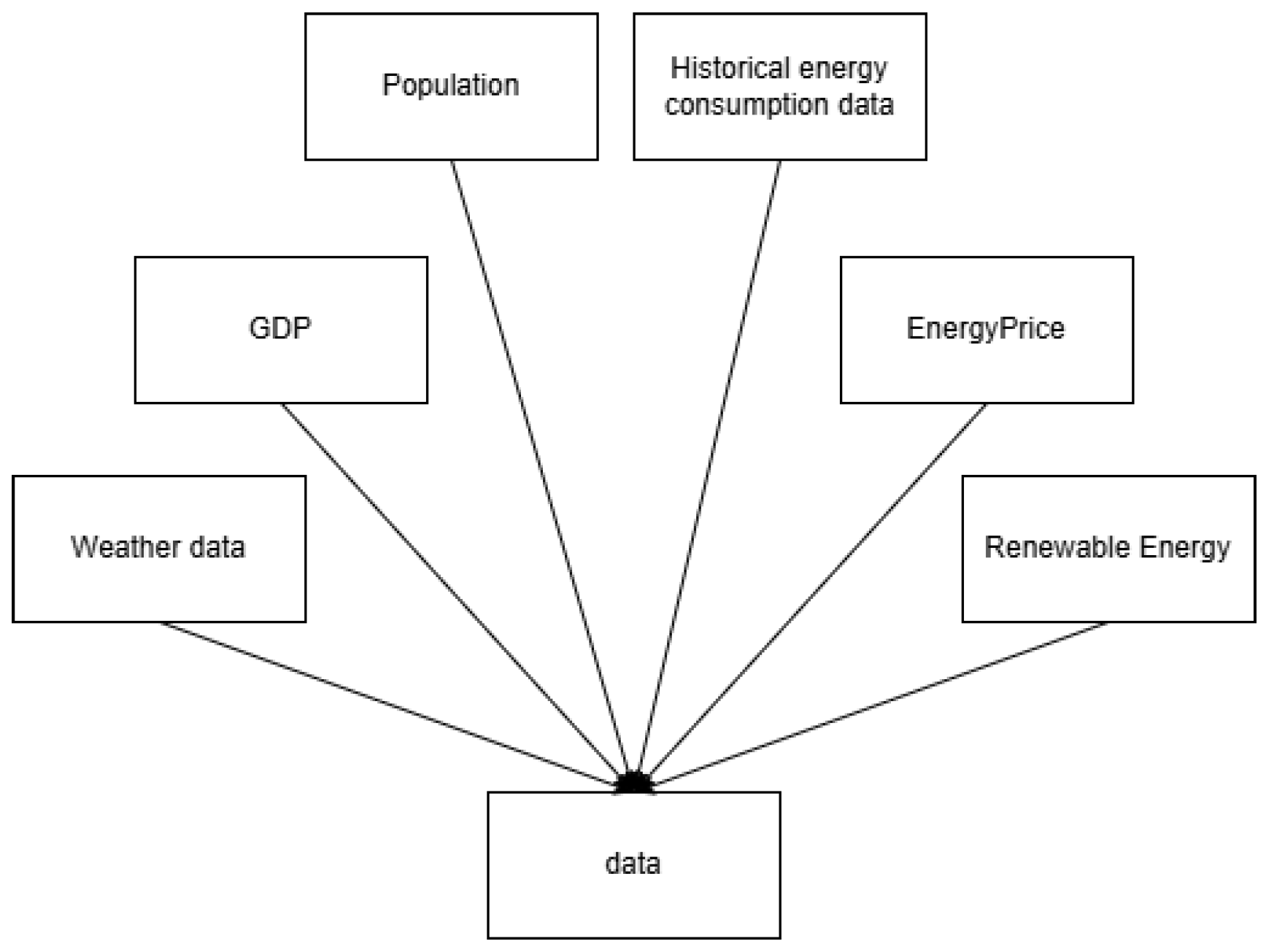
Figure 1.
Data Collection
3.2. EDA
EDA was performed on individual datasets as well as the combined dataset to uncover patterns, trends, and correlations among variables. This process provided insights into the relationships between energy demand and key influencing factors, such as weather conditions, socioeconomic indicators, and energy prices. By analyzing each dataset separately and in combination, potential dependencies and anomalies were identified, ensuring a more informed approach to feature selection and model development.
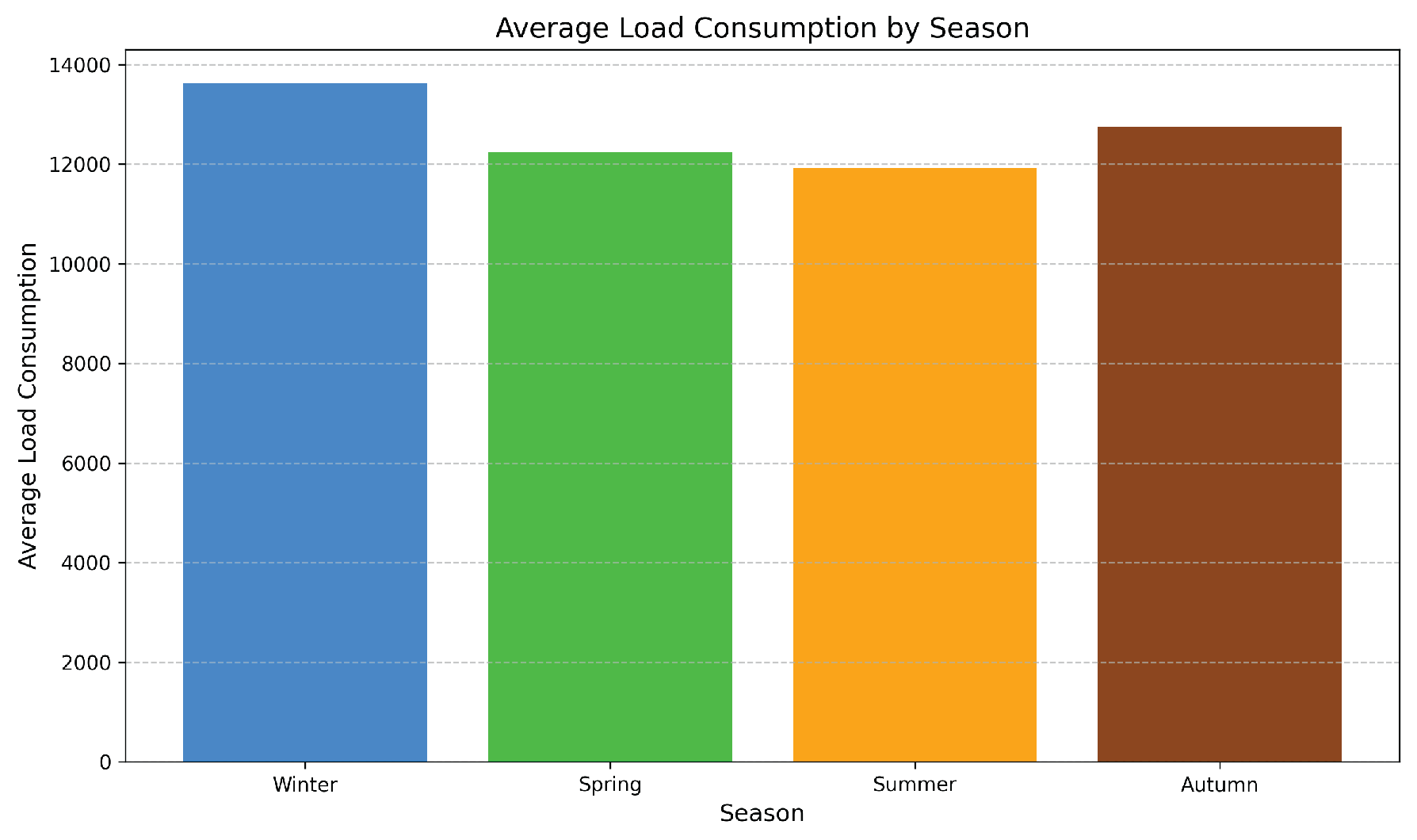
From Figure 2, it is evident that the data exhibits seasonality. To assess stationarity, the Augmented Dickey-Fuller (ADF) test was applied, confirming that the series is stationary [19,41]. Figure 3 and Figure 5 further illustrate that energy demand in the Netherlands tends to increase during the winter months. Additionally, Figure 4 shows a clear rise in energy demand during daytime hours.
Figure 2.
Load Consumption consumption 2015-2023, monthly average
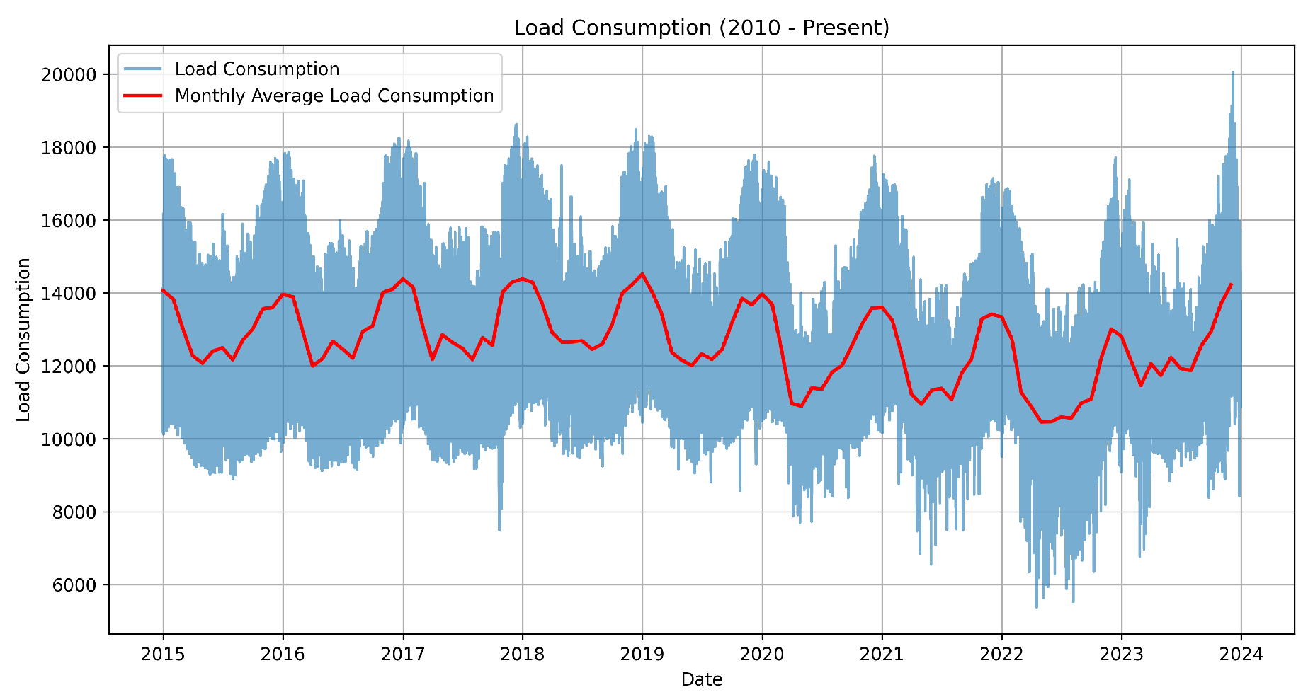
Figure 3.
Load Consumption consumption 2015-2023, monthly average
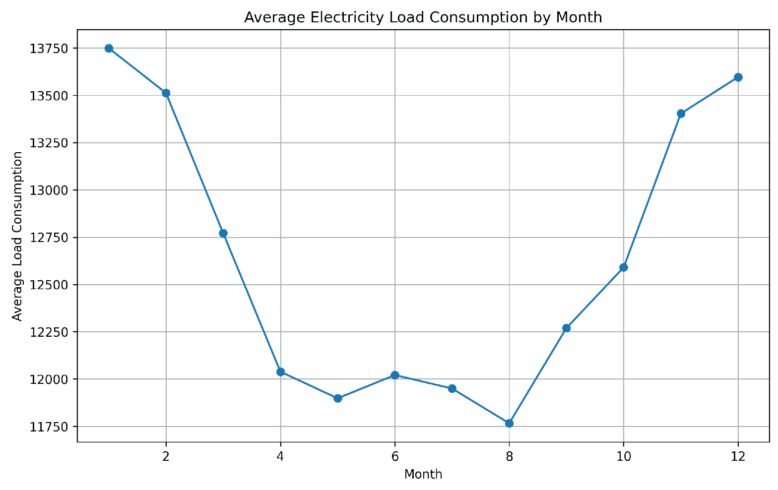
Figure 4.
average consumption of hour per day
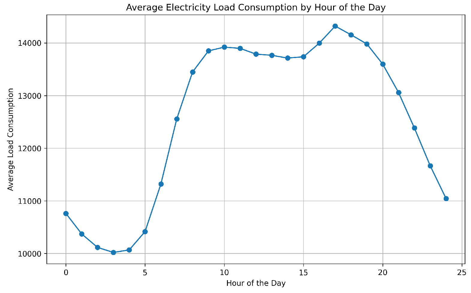
Figure 5.
Consumption per season
Noticeably, there is a rise in solar and wind energy consumption.
Figure 6.
Renwable Enegy Consumption in NL
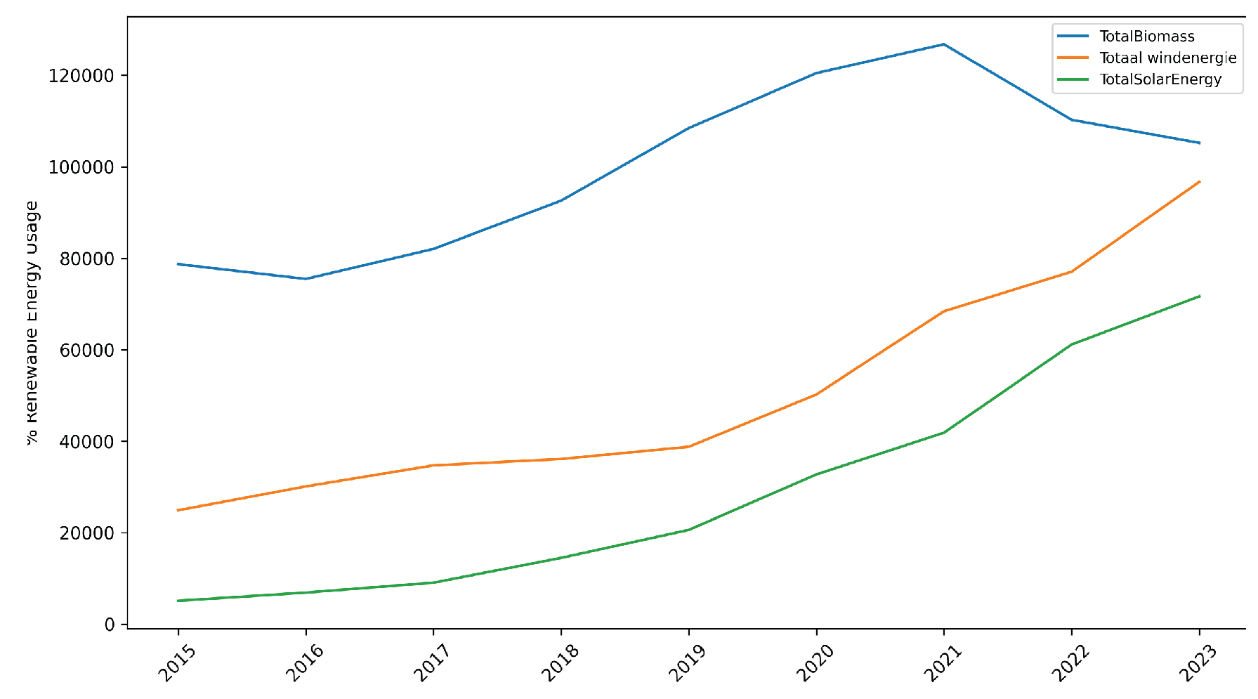
Figure 7.
Comparison of different rolling mean window sizes
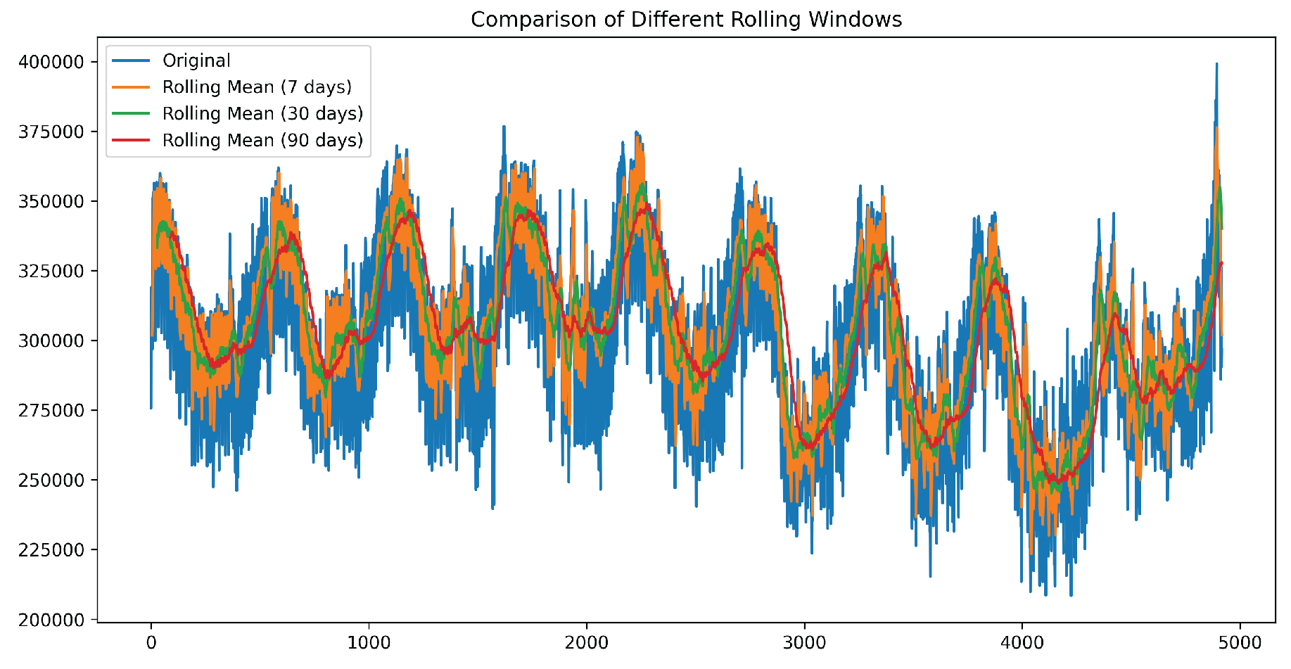
Figure 8.
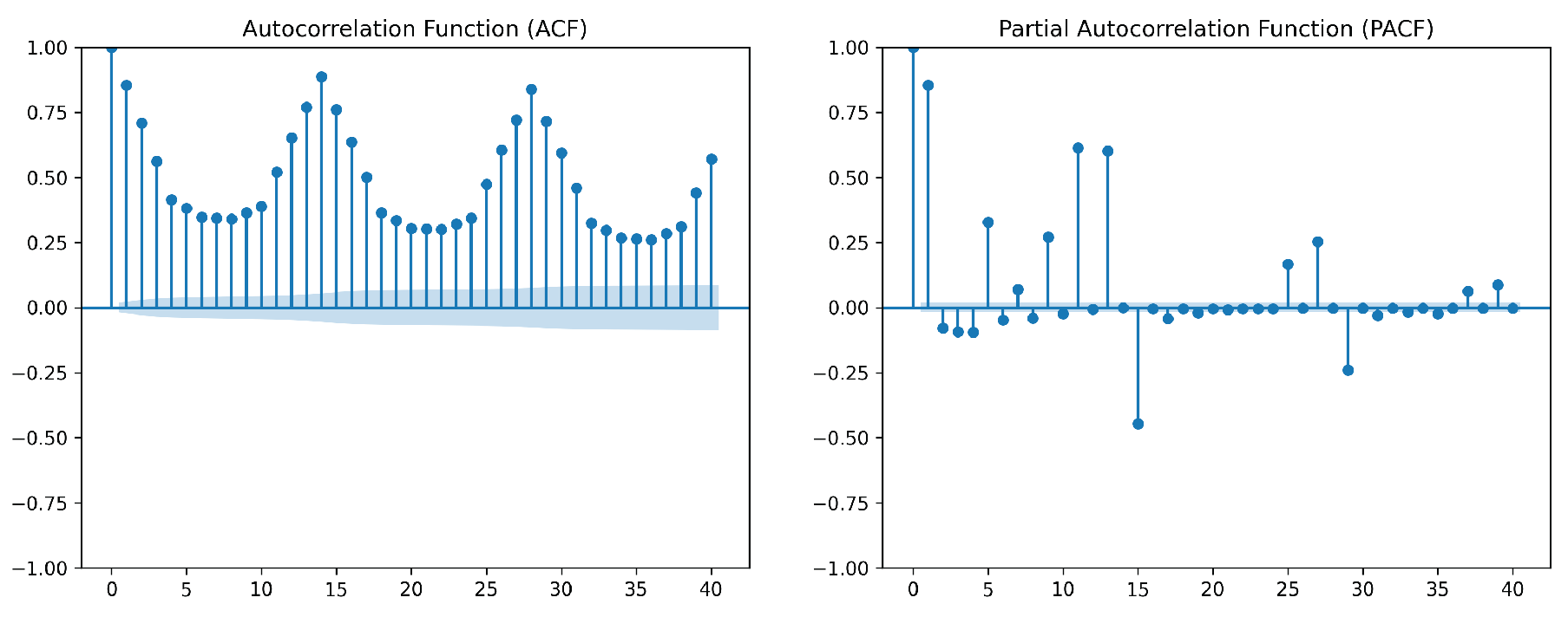
Autocorrelation Function (ACF), Partial Autocorrelation Function (PACF)
3.3. Data Cleaning and Preparation
Following the exploratory data analysis, the data must be refined to ensure consistency and reliability for modeling. This process involves identifying and handling outliers, addressing missing values, standardizing measurement units, and aligning data granularity across different sources.
3.3.1. Handling Missing Values
Data was almost complete; only 6 values out of 15,772 were missing in the ENTSO-E hourly data and were filled using the fill-forward method.
3.3.2. Handling Outliers
Outliers were identified using the Interquartile Range (IQR) method, with any data point exceeding 1.5 times the IQR flagged as an outlier. Given their minimal presence relative to the dataset, these outliers were addressed through Winsorization, capping values at the 1st and 99th percentiles to preserve data integrity while mitigating extreme variations.
3.3.3. Combining Data
The datasets were merged based on the date attribute. To address differences in temporal granularity, yearly data were upsampled to a daily frequency by forward-propagating the annual values across all days within the corresponding year.
3.3.4. Predictor Selection
Initially, 26 features were available for modeling. To refine the feature set, a three-step approach was applied:
- Correlation Matrix: This helped identify highly correlated variables, reducing redundancy in the dataset. By eliminating features that were strongly correlated with others, we minimized multicellularity and ensured that the model was not biased due to overlapping information.
- Variance Inflation Factor (VIF): VIF was used to quantify multicollinearity among predictors. Features with high VIF scores were removed to prevent instability in the model and improve interpretability. This step ensured that each predictor contributed unique information to the model without inflating standard errors.where is the coefficient of determination obtained by regressing on all other predictors.
- Principal Component Analysis (PCA):PCA was applied to reduce dimensionality and mitigate multicollinearity in both economic and renewable energy features. First, Population and GDP were standardized (mean=0, standard deviation=1) and then transformed into a single principal component, EconomicComponent, which explained approximately 93.8% of the variance in these economic indicators. Next, four renewable energy variables—TotalSolarEnergy, Totaal windenergie, TotalBiomass, and TotalRes(incl.Stat.Transfer)—were similarly scaled, and one principal component, RenewableEnergyComponent, captured about 92.6% of their combined variance. Finally, the original columns were optionally dropped to reduce redundancy, leaving the two new components to serve as lower-dimensional inputs for subsequent modeling.
3.3.5. Incorporating Rolling Mean Features
As part of feature engineering, rolling mean features were introduced to capture temporal trends in the data. Rolling means help smooth out short-term fluctuations and highlight longer-term trends, making them particularly useful for time series forecasting. By averaging past values over a specified window, rolling mean features reduce noise while preserving seasonality and trend components, ultimately improving model stability and predictive performance.
3.3.6. Feature Set Configurations
Three feature sets were tested in the experiments: Exogenous Features, focusing on meteorological data, energy prices, economic indicators, and renewable components; Generated Features, which include weekend/holiday flags and rolling windows to capture temporal patterns; and a Combined set containing both exogenous and generated features. This setup allowed for direct comparison of how each feature grouping contributes to forecasting performance.
3.3.7. Scaling Data
LSTMs are sensitive to feature magnitudes, so Min-Max Scaling is used to scale values between [0,1] or [-1,1], ensuring efficient gradient descent.
3.4. Model Implementation: Baseline Model SARIMAX
The Seasonal Autoregressive Integrated Moving Average with Exogenous Variables (SARIMAX) model was selected as the baseline for energy demand forecasting due to its effectiveness in capturing underlying trends, seasonal structures, and the influence of external covariates in time series data. As an extension of the classical ARIMA model, SARIMAX introduces seasonal components and allows for the incorporation of exogenous variables, making it particularly suitable for modeling electricity consumption patterns influenced by weather and socioeconomic factors.
SARIMAX captures temporal dependencies through autoregressive (AR) and moving average (MA) terms, stabilizes non-stationary trends via differencing (I), and accounts for recurring patterns through seasonal terms (S). The integration of exogenous regressors (X), such as weather and economic indicators, enables the model to enhance predictive performance by leveraging additional sources of information beyond the intrinsic time series behavior.
Hyperparameter Selection () and Seasonal Components
Model hyperparameters and seasonal components were identified through a combination of statistical testing, diagnostic plotting, and empirical evaluation:
- Stationarity: The Augmented Dickey-Fuller (ADF) test was conducted to assess stationarity. Since the test statistic rejected the null hypothesis of a unit root, the series was deemed stationary, and differencing order was set to .
- Short-Term Dynamics: The autocorrelation (ACF) and partial autocorrelation (PACF) functions were analyzed to determine p and q. The PACF exhibited significant lags at 1 and 2, suggesting , while the ACF revealed significant lags up to order 3, indicating (Figure 8).
- Seasonal Structure: Weekly seasonality was detected in the load patterns, motivating the choice of a seasonal period . Seasonal AR and MA terms were set to and , respectively. As the data was already stationary, seasonal differencing was not required, and .
A grid-based trial-and-error approach was used to fine-tune the model within the identified ranges, with selection based on minimizing forecasting error. The final model specification, , provided a well-balanced fit that effectively captured both short-term variations and seasonal patterns.
3.5. Hybrid Multi-Stage Forecasting Model
This study implements a hybrid multi-stage forecasting framework, combining a SARIMAX model with an LSTM network. The rationale behind using a hybrid approach is to exploit the complementary strengths of traditional statistical methods and deep learning techniques. The methodology is structured into two primary modeling stages: the SARIMAX model, previously discussed, which handles linear and seasonal components, and the LSTM network, which addresses complex non-linear patterns not captured by the initial stage [42].
3.5.1. Stage 2: LSTM Network (Residual Modeling)
In the second stage of the hybrid forecasting framework, LSTM network is employed to model the complex non-linear dependencies present in the residuals generated by the SARIMAX model. These residuals capture the discrepancies between the observed energy load and the SARIMAX predictions—i.e., the signal components not adequately explained by linear or seasonal trends.
To effectively model these residual patterns, a sliding window technique is applied, converting the one-dimensional residual time series into sequential input-output pairs suitable for supervised learning with LSTM. Specifically, for each time step t, the input to the LSTM is a sequence of the previous 30 residuals:
and the target output is the residual at time t, . This sequence structure preserves temporal dependencies and enables the LSTM to learn long-range relationships in the residual patterns.
Unlike feedforward neural networks, which treat input vectors independently, LSTM networks process these sliding windows as sequential data. The residuals are not flattened into feature vectors; instead, each sequence is shaped as a 2D array with dimensions (window_length, 1), where each time step contains one feature (the residual value).
The LSTM architecture used in this study consists of:
- A single LSTM layer with 50 units and ReLU activation.
- A Dense output layer to predict the next residual.
The network is trained using the Mean Squared Error (MSE) loss function and optimized with the Adam optimizer. After training, the model recursively generates predictions for future residuals over the desired forecasting horizon. These predicted residuals are then added to the original SARIMAX forecasts to obtain the final energy demand predictions:
This hybrid approach effectively addresses both the linear-seasonal trends (via SARIMAX) and non-linear variations (via LSTM).
3.6. Sequence-to-Sequence Forecasting Model
To complement the hybrid approach, a seq-to-seq model architecture was implemented to directly forecast energy consumption over multiple time horizons. This model leverages two separate Long Short-Term Memory (LSTM) networks to form an encoder-decoder structure, enabling it to capture complex temporal dependencies in multivariate time series data. seq-to-seq models are particularly suited for forecasting tasks where both input and output sequences can vary in length, offering flexibility for short-term and long-term predictions.
3.6.1. Encoder
The encoder processes the historical input features and summarizes them into a fixed-length context vector. The input to the encoder is a 3D tensor of shape (samples,input_length, num_encoder_feature), where each sample represents a sequence of multivariate past observations.
The encoder architecture consists of a single LSTM layer with 64 units. This layer outputs the final hidden state () and cell state (), which encapsulate the temporal context of the input sequence. These states are then passed to the decoder to initialize its internal memory.
3.6.2. Decoder
The decoder receives a sequence of lagged target values as input, shaped as (samples, output_length, num_decoder_feature). These values are scaled using Min-Max normalization. During training, teacher forcing is employed, which means the true previous target values are used as decoder inputs to guide the learning process and reduce error accumulation.
The decoder also uses a single LSTM layer with 64 units, initialized with the encoder’s hidden and cell states. Its outputs are passed through a TimeDistributed(Dense(1)) layer, which applies a fully connected layer to each time step individually, producing one forecasted value per future time step.
3.6.3. Training Configuration and Model Details
The model was built using the Keras functional API, enabling distinct inputs for the encoder and decoder. The following hyperparameters and training settings were used:
- Input length: 30 days
- Output length: 7 days
- LSTM units: 64 for both encoder and decoder
- Number of LSTM layers: 1 in both encoder and decoder
- Training technique: Teacher forcing
- Batch size: 16
- Epochs: 20
- Loss function: Mean Squared Error (MSE)
- Optimizer: Adam
- Decoder input during training: Lagged target values (scaled)
All features, including the target variable, were scaled to the range using Min-Max scaling to enhance model convergence. After prediction, inverse transformation is applied to return the forecasted values to their original scale.
3.7. Model Evaluation
1. Root Mean Squared Error (RMSE) RMSE is calculated as the square root of the average squared differences between the predicted and actual values. Because it squares the errors before averaging, it penalizes larger deviations more strongly [43]. In energy demand forecasting, where sudden large errors (for example, unexpected demand spikes) can have significant operational consequences, RMSE helps highlight these potentially critical mistakes. Moreover, since its units match those of the target variable (e.g., megawatts), it provides an intuitive sense of the error magnitude.
2. Mean Absolute Percentage Error (MAPE) MAPE represents the average absolute difference between the actual and predicted values expressed as a percentage of the actual values [43]. This percentage-based error measure is useful because it normalizes the error, allowing for comparisons across different scales or time periods. In energy demand forecasting, where values can vary widely depending on time and context, MAPE provides stakeholders with an easily understandable measure of relative error—making it clear, for example, that forecasts are off by an average of X%
3. Mean Absolute Error (MAE)MAE computes the average absolute difference between predicted and actual values. Unlike RMSE, MAE treats all errors equally without disproportionately penalizing larger errors [43]. This quality makes it a robust indicator of average performance and is particularly useful in energy forecasting when it’s important to understand the typical deviation without being overly influenced by a few extreme cases. It provides a clear interpretation of the typical forecasting error in the same units as the target variable.
Using these metrics in combination allows for a comprehensive evaluation of model performance. RMSE and MAE offer insights into the magnitude of forecasting errors, while MAPE provides a normalized error measure that is easier to communicate to decision makers. This multi-faceted evaluation is critical in energy demand prediction, where both absolute error magnitudes and relative error percentages have direct implications on grid management and planning.
4. Normalized RMSE and MAE To ensure meaningful interpretation and fair comparison across models and forecast horizons, both RMSE and MAE were normalized by dividing them by the mean of the actual load values for each forecast horizon. This yields scale-independent metrics—normalized RMSE (nRMSE) and normalized MAE (nMAE)—which express the average error as a proportion of the typical energy demand.
This normalization is particularly important in energy forecasting contexts, where the absolute magnitude of load values can vary significantly across seasons, time periods, or scenarios. Without normalization, RMSE and MAE may appear deceptively large due to the high numerical scale of the target variable (e.g., megawatts). Presenting normalized metrics therefore allows for a clearer understanding of model performance relative to the demand level and facilitates more equitable comparisons across models and feature sets [44].
Normalized error metrics are also commonly recommended in time series forecasting literature, especially when communicating results to stakeholders who may find relative error more intuitive than raw unit-based deviations.

Table 1.
Performance metrics used to evaluate models.
| Metric | Formula | Interpretation |
|---|---|---|
| RMSE | Measures average error magnitude. | |
| MAPE | Measures percentage error. | |
| MAE | Measures average absolute error. |
4. Results
This section presents the results of the three models evaluated in this study across different feature configurations. It also addresses the impact of renewable and socioeconomic features on forecasting accuracy.
4.1. Performance of Baseline SARIMAX
The performance of the SARIMAX model using different feature sets is summarized in Table 2.
Overall, using only exogenous features led to poor performance, with an nRMSE of 11.14% and a MAPE of 8.81%, indicating the model struggled to capture meaningful patterns. Generated features improved predictive accuracy substantially (nRMSE = 4.00%, MAPE = 3.09%), while combining both feature types led to a slight improvement (nRMSE = 3.96%, MAPE = 3.01%).
4.2. SARIMAX-LSTM: Hybrid Model Performance
The SARIMAX-LSTM model exhibited improved and stable performance over the baseline SARIMAX, particularly with generated and combined feature sets. Table 3 outlines the performance at the 180-day prediction horizon.
Using only exogenous features yielded poor results (nRMSE = 12.13%, MAPE = 9.89%). Generated features enhanced accuracy significantly (nRMSE = 4.18%, MAPE = 3.38%), while the combined set slightly improved further (nRMSE = 3.84%, MAPE = 3.13%).
4.3. Sequence to Sequence Performance
The Seq2Seq model consistently outperformed the other models across all feature configurations, particularly at the 180-day horizon. Table 4 summarizes these results. Generated features yielded the best accuracy (nRMSE = 2.86%, MAPE = 1.88%). Exogenous features resulted in higher errors (nRMSE = 3.66%, MAPE = 2.61%), while combining both feature types slightly worsened performance (nRMSE = 3.19%, MAPE = 2.29%).
4.4. Summary Models Results
Among the evaluated models, the Seq2Seq model with generated features achieved the best performance, highlighting the effectiveness of deep learning in capturing complex sequential patterns. It consistently outperformed the classical and hybrid models in both short- and long-term horizons.
To further illustrate the performance differences, Figure 9 shows a side-by-side comparison of MAPE across all three models and feature sets.
4.5. Impact of Exogenous Feature Sets
To assess the impact of renewable and socioeconomic indicators, additional SARIMAX experiments were conducted.
At the 1-day horizon, renewable energy features improved accuracy significantly (MAPE reduced from 2.18% to 1.09%), while socioeconomic features slightly worsened predictions (MAPE = 2.48%). At the 180-day horizon, both feature sets increased error, suggesting limited utility for long-term forecasting (Table 5).
5. Discussion
This section critically reflects on the study’s findings, comparing them with previous work, analyzing the strengths and weaknesses of the models and features explored, and addressing limitations and ethical implications of energy demand forecasting.
5.1. Performance Comparison and Insights
1. Exogenous Features Only. Models trained exclusively on exogenous variables, such as weather, energy prices, and socioeconomic indicators, consistently underperformed across all forecast horizons. For example, SARIMAX yielded a MAPE of 8.81% and SARIMAX-LSTM scored 9.89%, while Seq2Seq slightly improved at 2.61%. These results indicate that while these features provide contextual insight, they fail to capture internal demand dynamics on their own.
2. Generated Features Only. Internally generated features, such as calendar-based variables and rolling demand windows, led to significantly improved accuracy across all models. SARIMAX achieved a MAPE of 3.09%, SARIMAX-LSTM reached 3.38%, and Seq2Seq performed best at 1.88%. This highlights the dominant role of historical patterns and temporal structure in determining energy demand.
3. Combined Feature Set. Combining generated and exogenous features provided marginal improvements over generated features alone in some cases (e.g., SARIMAX: 3.01%, SARIMAX-LSTM: 3.13%), but slightly worsened Seq2Seq performance (MAPE increased from 1.88% to 2.29%). This suggests that while combining signals may be beneficial for statistical models, deep learning architectures may become more sensitive to noise introduced by less predictive external features.
4. Deep Learning Performance. Among the evaluated models, Seq2Seq demonstrated the most robust and consistent performance, particularly at the 180-day forecast horizon. With the lowest nRMSE (2.86%) and MAPE (1.88%) when using generated features, it significantly outperformed SARIMAX (3.96%, 3.01%) and SARIMAX-LSTM (3.84%, 3.13%). This supports the strength of deep learning in modeling long-term temporal dependencies when fed clean, structured input data.
6. Conclusions
The findings demonstrate that combining exogenous and engineered features substantially improves forecasting accuracy, particularly when tailored to the strengths of each model architecture. The SARIMAX model captured seasonal trends effectively, while the SARIMAX–LSTM hybrid improved short-term accuracy by modeling nonlinear fluctuations. The sequence-to-sequence (Seq2Seq) deep learning model offered robust long-range forecasting performance, especially when trained with calendar-based and smoothed historical features.
Experiments confirmed that including renewable energy variables, such as wind and solar production, significantly reduced long-term prediction error, highlighting their growing influence on national energy dynamics. Socioeconomic indicators like GDP and population also contributed modest improvements, especially when forecasting over multi-month horizons.
Beyond quantitative improvements, this work illustrates the value of feature engineering and model layering in building scalable, adaptable forecasting systems. These insights are particularly relevant for grid operators and policymakers, as they transition toward a decentralized and renewables-driven energy landscape.
This study developed and evaluated a hybrid multi-stage forecasting framework to enhance short- and long-term electricity demand prediction in the Netherlands. By integrating statistical (SARIMAX), hybrid (SARIMAX–LSTM), and deep learning (sequence-to-sequence) models with diverse data sources, including weather, energy prices, socioeconomic indicators, and engineered temporal features, the research sought to overcome the limitations of single-model forecasting systems.
The results showed that engineered time-series features (e.g., rolling averages, calendar effects) consistently improved model performance across different architectures. Among the evaluated models, the sequence-to-sequence architecture, trained with generated features, achieved the best forecasting accuracy (MAPE = 1.88% at the 180-day horizon), outperforming both classical and hybrid approaches.
While the study is constrained by its focus on one country and specific modeling choices, it provides evidence that engineered temporal features combined with appropriate model architectures can meaningfully improve energy demand forecasting. These findings may support future research and practical forecasting efforts as energy systems grow more dynamic and data-driven.
References
- Altinay, G.; Karagol, E. Electricity consumption and economic growth: Evidence from Turkey. Energy Economics 2005, 27, 849–856. [CrossRef]
- González Grandón, T.; Schwenzer, J.; Steens, T.; Breuing, J. Electricity demand forecasting with hybrid classical statistical and machine learning algorithms: Case study of Ukraine. Applied Energy 2024, 355, 122249. [CrossRef]
- IEA. Growth in global electricity demand is set to accelerate in the coming years as power-hungry sectors expand 2025.
- Song, H.; Zhang, B.; Jalili, M.; Yu, X. Multi-swarm multi-tasking ensemble learning for multi-energy demand prediction. Applied Energy 2025, 377, 124553. [CrossRef]
- NOS. Netbeheerder: na 2030 grotere kans op prijspieken door stroomtekorten 2024.
- IEA, Inc.. IEA report highlights the Netherlands’ opportunities to drive further progress in its clean energy transition. IEA 2025.
- Tennet. No extra space on electricity grid in large part of Noord-Holland next decade 2024.
- Vivas, E.; Allende-Cid, H.; Salas, R. A systematic review of statistical and machine learning methods for electrical power forecasting with reported mape score. Entropy 2020, 22, 1412. [CrossRef]
- Islam, M.; Che, H.S.; Hasanuzzaman, M.; Rahim, N. Chapter 5 - Energy demand forecasting. In Energy for Sustainable Development; Hasanuzzaman, M.; Rahim, N.A., Eds.; Academic Press, 2020; pp. 105–123. [CrossRef]
- Tiwari, S.; Jain, A.; Ahmed, N.M.O.S.; Charu.; Alkwai, L.M.; Dafhalla, A.K.Y.; Hamad, S.A.S. Machine learning-based model for prediction of power consumption in smart grid-smart way towards smart city. Expert Systems 2022, 39, e12832. [CrossRef]
- Colussi, E. An integrated modeling approach to provide flexibility and sustainability to the district heating system in South-Holland, the Netherlands. 2024.
- Suganthi, L.; Samuel, A.A. Energy models for demand forecasting—A review. Renewable and Sustainable Energy Reviews 2012, 16, 1223–1240. [CrossRef]
- P. Scheres, c.K. Laagste gasverbruik in 50 jaar: “Bezuinigen vaak noodzakelijk. RTL Nieuws & Entertainment 2023.
- Liu, J.; Wang, S.; Wei, N.; Chen, X.; Xie, H.; Wang, J. Natural gas consumption forecasting: A discussion on forecasting history and future challenges. Journal of Natural Gas Science and Engineering 2021, 90, 103930. [CrossRef]
- Kim, C.H.; Kim, M.; Song, Y.J. Sequence-to-sequence deep learning model for building energy consumption prediction with dynamic simulation modeling. Journal of Building Engineering 2021, 43, 102577. [CrossRef]
- Jain, R.K.; Smith, K.M.; Culligan, P.J.; Taylor, J.E. Forecasting energy consumption of multi-family residential buildings using support vector regression: Investigating the impact of temporal and spatial monitoring granularity on performance accuracy. Applied Energy 2014, 123, 168–178. [CrossRef]
- Han, Z.; Zhao, J.; Leung, H.; Ma, K.F.; Wang, W. A review of deep learning models for time series prediction. IEEE Sensors Journal 2019, 21, 7833–7848. [CrossRef]
- Yamak, P.T.; Yujian, L.; Gadosey, P.K. A Comparison between ARIMA, LSTM, and GRU for Time Series Forecasting. In Proceedings of the Proceedings of the 2019 2nd International Conference on Algorithms, Computing and Artificial Intelligence, New York, NY, USA, 2020; ACAI ’19, p. 49–55. [CrossRef]
- Alharbi, F.R.; Csala, D. A Seasonal Autoregressive Integrated Moving Average with Exogenous Factors (SARIMAX) Forecasting Model-Based Time Series Approach. Inventions 2022, 7. [CrossRef]
- de Gooyert, V.; de Coninck, H.; ter Haar, B. How to make climate policy more effective? The search for high leverage points by the multidisciplinary Dutch expert team ‘Energy System 2050’. Systems Research and Behavioral Science 2024, [https://onlinelibrary.wiley.com/doi/pdf/10.1002/sres.3039]. [CrossRef]
- Sarkodie, S.A. Estimating Ghana’s electricity consumption by 2030: An ARIMA forecast. Energy Sources, Part B: Economics, Planning, and Policy 2017, 12, 936–944. [CrossRef]
- Netherlands, S. Dutch economy grows by 0.4 percent in Q4 2024. Statistics Netherlands 2025.
- Statista. Total population of the Netherlands 2029, 2024.
- van Algemene Zaken, M. Package of measures to cushion the impact of rising energy prices and inflation. News Item | Government.nl 2022.
- Mir, A.A.; Alghassab, M.; Ullah, K.; Khan, Z.A.; Lu, Y.; Imran, M. A Review of Electricity Demand Forecasting in Low and Middle Income Countries: The Demand Determinants and Horizons. Sustainability 2020, 12. [CrossRef]
- van de Sande, S.N.; Alsahag, A.M.; Mohammadi Ziabari, S.S. Enhancing the Predictability of Wintertime Energy Demand in The Netherlands Using Ensemble Model Prophet-LSTM. Processes 2024, 12, 2519. [CrossRef]
- Kočí, J.; Kočí, V.; Maděra, J.; Černỳ, R. Effect of applied weather data sets in simulation of building energy demands: Comparison of design years with recent weather data. Renewable and Sustainable Energy Reviews 2019, 100, 22–32. [CrossRef]
- Zhong, W.; Zhai, D.; Xu, W.; Gong, W.; Yan, C.; Zhang, Y.; Qi, L. Accurate and efficient daily carbon emission forecasting based on improved ARIMA. Applied Energy 2024, 376, 124232. [CrossRef]
- Tian, N.; Shao, B.; Bian, G.; Zeng, H.; Li, X.; Zhao, W. Application of forecasting strategies and techniques to natural gas consumption: A comprehensive review and comparative study. Engineering Applications of Artificial Intelligence 2024, 129, 107644. [CrossRef]
- Agyare, S.; Odoi, B.; Wiah, E.N. Predicting Petrol and Diesel Prices in Ghana, A Comparison of ARIMA and SARIMA Models. Asian Journal of Economics, Business and Accounting 2024, 24, 594–608. [CrossRef]
- Koukaras, P.; Bezas, N.; Gkaidatzis, P.; Ioannidis, D.; Tzovaras, D.; Tjortjis, C. Introducing a novel approach in one-step ahead energy load forecasting. Sustainable Computing: Informatics and Systems 2021, 32, 100616. [CrossRef]
- Kaur, S.; Bala, A.; Parashar, A. A multi-step electricity prediction model for residential buildings based on ensemble Empirical Mode Decomposition technique. Science and Technology for Energy Transition 2024, 79, 7. [CrossRef]
- Sen, D.; Hamurcuoglu, K.I.; Ersoy, M.Z.; Tunç, K.M.; Günay, M.E. Forecasting long-term world annual natural gas production by machine learning. Resources Policy 2023, 80, 103224. [CrossRef]
- Yesilyurt, H.; Dokuz, Y.; Dokuz, A.S. Data-driven energy consumption prediction of a university office building using machine learning algorithms. Energy 2024, 310, 133242. [CrossRef]
- Md Ramli, S.S.; Nizam Ibrahim, M.; Mohamad, A.; Daud, K.; Saidina Omar, A.M.; Darina Ahmad, N. Review of Artificial Neural Network Approaches for Predicting Building Energy Consumption. In Proceedings of the 2023 IEEE 3rd International Conference in Power Engineering Applications (ICPEA), 2023, pp. 328–333. [CrossRef]
- Gaweł, B.; Paliński, A. Global and Local Approaches for Forecasting of Long-Term Natural Gas Consumption in Poland Based on Hierarchical Short Time Series. Energies 2024, 17. [CrossRef]
- Koninklijk Nederlands Meteorologisch Instituut. KNMI.
- Centraal Bureau voor de Statistiek (CBS). CBS. GDP data source.
- Centraal Bureau voor de Statistiek (CBS). CBS. population data source.
- Centraal Bureau voor de Statistiek (CBS). CBS. energy price data source.
- Naik, K. Hands-On Python for Finance: A practical guide to implementing financial analysis strategies using Python; Packt Publishing Ltd, 2019.
- Sheng, F.; Jia, L. Short-term load forecasting based on SARIMAX-LSTM. In Proceedings of the 2020 5th International Conference on Power and Renewable Energy (ICPRE). IEEE, 2020, pp. 90–94.
- Saigal, S.; Mehrotra, D. Performance comparison of time series data using predictive data mining techniques. Advances in Information Mining 2012, 4, 57–66.
- Botchkarev, A. Performance metrics (error measures) in machine learning regression, forecasting and prognostics: Properties and typology. arXiv preprint arXiv:1809.03006 2018.
Figure 9.
MAPE results- Different models
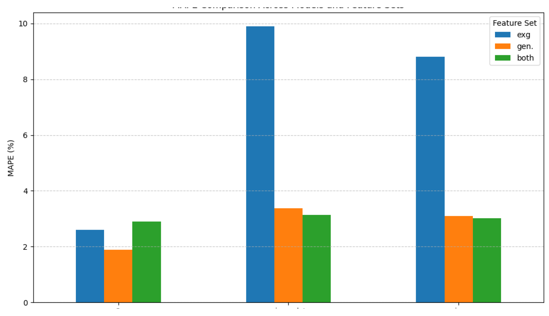
Table 2.
Performance comparison of SARIMAX with different feature sets.
| Metric | Exog. Features | Gen. Features | Both |
|---|---|---|---|
| nRMSE% | 11.14 | 4.00 | 3.96 |
| MAPE | 8.81 | 3.09 | 3.01 |
| nMAE% | 9.16 | 3.01 | 2.94 |
Table 3.
Performance comparison of SARIMAX-LSTM with different feature sets- Horizon = 180 days
| Metric | Exog. Features | Gen. Features | Both |
|---|---|---|---|
| nRMSE% | 12.13 | 4.18 | 3.84 |
| MAPE% | 9.89 | 3.38 | 3.13 |
| nMAE% | 10.728 | 3.33 | 3.09 |
Table 4.
Performance comparison of sequence to sequence- Horizon = 180 days
| Metric | Exog. Features | Gen. Features | Both |
|---|---|---|---|
| nRMSE% | 3.66 | 2.86 | 3.19 |
| MAPE% | 2.617 | 1.88 | 2.29 |
| nMAE% | 2.55 | 2.29 | 2.22 |
Table 5.
Forecast accuracy comparison with and without renewable energy features & socioeconomic features.
Table 5.
Forecast accuracy comparison with and without renewable energy features & socioeconomic features.
| Horizon | Features | nRMSE (%) | nMAE (%) | MAPE (%) |
|---|---|---|---|---|
| 1 day | Without exo. | 2.18 | 2.18 | 2.18 |
| 1 day | With Renewables | 1.09 | 1.09 | 1.09 |
| 1 day | With Soscio. | 2.48 | 2.48 | 2.48 |
| 180 days | Without exo. | 7.85 | 6.67 | 6.90 |
| 180 days | With Renewables | 9.07 | 7.54 | 7.93 |
| 180 days | With Soscio. | 8.72 | 7.34 | 7.26 |
Disclaimer/Publisher’s Note: The statements, opinions and data contained in all publications are solely those of the individual author(s) and contributor(s) and not of MDPI and/or the editor(s). MDPI and/or the editor(s) disclaim responsibility for any injury to people or property resulting from any ideas, methods, instructions or products referred to in the content. |
© 2025 by the authors. Licensee MDPI, Basel, Switzerland. This article is an open access article distributed under the terms and conditions of the Creative Commons Attribution (CC BY) license (http://creativecommons.org/licenses/by/4.0/).
Copyright: This open access article is published under a Creative Commons CC BY 4.0 license, which permit the free download, distribution, and reuse, provided that the author and preprint are cited in any reuse.


