
Submitted:
10 October 2024
Posted:
11 October 2024
You are already at the latest version
Abstract
Short-term electrical demand forecasting is crucial for the effective operation of new electrical networks. This necessity arises from the requirement for more timely demand information compared to traditional networks, as well as the integration of new energy sources into the electrical grid. Most existing forecasting methodologies fail because they do not consider the nonlinearities of the system, and because they neglect to represent important external influences on the problem; in other words, they are not based on a holistic approach to electricity demand forecasting. In this study, we present a new approach to developing an electrical demand forecasting model, and consider a case study to evaluate the importance of several factors affecting electricity consumption and forecast accuracy. We use an ISO NE (Independent System Operator New England) dataset that represents the total electrical load of several New England cities from January 2017 to December 2019. This dataset includes 23 independent variables, such as meteorological data, economic indicators and market information. Our study presents a pipeline for building electrical demand forecast models using time series information as input. By carefully selecting variables and representing external factors, we demonstrate the feasibility of generating a more accurate forecasting model with reduced computational resources. Our results show that incorporating external factors can enhance model accuracy by up to 60%. To handle large input datasets, variable selection is crucial for reducing dimensionality while maintaining accuracy, enabling the effective application of deep learning models. Simulations reveal that deep learning models with no more than three intermediate layers and an optimal number of neurons perform efficiently. The CNN+LSTM composite model achieved the lowest error rate at 0.15%, surpassing previously studied models, including standalone CNN and LSTM approaches, which had error rates of 0.8% and 1.44%, respectively. The CNN's feature extraction abilities, combined with the LSTM's strength in handling time-series data, were instrumental in achieving superior performance across most scenarios.
Keywords:
electricity forecasting model
; deep learning
; computational intelligence
1. Introduction
The traditional structure of the electrical power system is characterized by the presence of large power generation plants (such as hydroelectric and thermal power plants) located far from consumption areas. In this type of system, decisions are centralized and the flow of energy is unidirectional, from the operators to the end consumers.
However, changes in the electrical matrix have been driven by a growing proportion of clean and sustainable sources, spurred by the deregulation of the sector, and these are reshaping the terrain of electric power grid management. We are moving from a scenario involving stable predictions and controlled power generation to a more volatile and less predictable scenario where the flow of energy is bidirectional, from operators to consumers and vice versa [1].
Modern electric networks, referred to as “smart grids”, represent an evolution designed to address contemporary challenges by leveraging advanced communication and information technologies. These networks encompass not only the transmission of energy from generation to substations but also the distribution of electricity from substations to individual end-users [2].
In a smart grid, electricity demand forecasting and distributed electricity generation forecasting play key roles in terms of maintaining grid stability, preventing overloads, and ensuring a smooth transition to environmentally sustainable energy use. The ability to understand and predict energy supply and demand is crucial [3].
In [4] , the researchers identified two categories of demand: individual consumer demand and aggregate demand. Aggregate demand is forecast based on the hierarchy of elements in the network and the sum of the individual demand hours from various consumers. Consequently, the geographical scope of application of a model will depend on the network hierarchy to which the input data correspond.
The current sparse interconnections of alternative electricity sources and the demand they serve requires distributed control and monitoring of power flow, which necessitates a higher level of availability of information for effective decision-making. Decision-making can be of two types: (a) unit commitments and (b) load dispatch [5,6]. Load dispatch involves the instantaneous allocation of power generation to meet demand in real time or at very short intervals (with lead times of several minutes to a couple of hours). It requires continual adjustments to power generation to match fluctuations in electricity demand and variations in supply, especially when incorporating renewable energy sources like solar and wind, which can be intermittent and unpredictable. Unit commitment involves deciding which generating units will be connected and available to operate over a longer time horizon, with lead times of several hours or days. These processes involve electricity demand forecasting on a longer time scale. Unit commitment decisions are based on hourly or daily demand forecasts, and do not require adjustments as frequently as load dispatch.
Various methodologies exist for energy forecasting, such as the procedure proposed in [7,8] for predicting electricity generation and [3,4,9] for predicting electricity demand. One aspect that is common to many new models is the use of machine learning techniques, which are important for electricity demand forecasting due to their ability to handle complex, nonlinear relationships and large datasets, which traditional statistical methods often struggle to handle. Within this context deep learning has emerged as a transformative technology in pattern recognition tasks, particularly in complex, high-dimensional data. Its ability to automatically learn from large datasets and adapt to various applications has made it indispensable in fields such as financial fraud detection, medical imaging, and power systems research [9]. By analyzing historical data, weather conditions, socio-economic factors, and other relevant information, these techniques can accurately predict both short-term and long-term electricity demand. Models such as DNNs, LSTMs, and their combinations are particularly well-suited for applications in electrical power systems [9].
This paper focuses on developing an electricity demand forecasting methodology based on machine learning techniques. Building such models is complex, as the designer needs to make numerous decisions [10]. The objective of this article is to simplify this process by identifying the key aspects and providing guidance on handling them when assembling the model. To demonstrate the importance of the components of the model, a case study is presented with varying input variables, parameters, and model structures.
The main contributions of this paper can be summarized as follows: (1) we em-phasize the growing importance of short-term electricity demand forecasting; (2) we present a comprehensive framework detailing the construction of electrical demand forecasting models; (3) we address critical considerations in the development of elec-trical demand forecasting models; and (4) we evaluate the effectiveness of our model through an analysis of its representation of demand-affecting factors and the efficacy of relevant forecasting methodologies.
2. Electricity Demand Forecasting
2.1. Electricity Demand
Electrical energy consumption is subject to a multitude of influencing factors, such as user behaviors, weather conditions, seasonal variations, and economic indicators [11]. The nonlinear nature of the relationship between exogenous factors and electricity consumption adds complexity to electricity prediction processes.
The complexities of electricity prediction also depend on the granularity of the demand forecast. The prediction of aggregate consumer demand has proven to be more manageable than individual consumer demand, due to stronger correlations with external factors like temperature, humidity, and internal factors such as historical trends. Aggregation mitigates the inherent volatility arising from individual consumers, resulting in a smoother curve shape and greater homogeneity [5].
In [12], two situations were compared, one where predictions were carried out for individual users and an aggregate prediction was generated from these, and another where the prediction of the electrical load was made directly from the aggregate demand.
With regard to reducing electricity consumption, it is important to take into account the use of strategies to control the temperature of buildings and to reduce costs by taking advantage of surplus photovoltaic energy, as proposed in [13].
2.2. Selection of Forecasting Methodologies
2.2.1. Forecasting Methodologies Based on Time Series
One of the possible ways to predict electricity consumption is through time series analysis. Time series data enable future values to be predicted based on past values with a certain margin of error [14].
Traditional methodologies for electricity demand forecasting include statistical time series models such as ARIMA (autoregressive integrated moving average), SARIMA (seasonal ARIMA), and exponential smoothing. In [15], these techniques were described as benchmarks in the field of electricity demand forecasting. In recent decades, however, computational intelligence methods have gained prominence, as they are better able to describe the trends in nonlinear systems and take into account the effects of exogenous factors. As examples, we can mention artificial neural networks (ANNs), support vector machine (SVM) and other approaches.
Recent works published over the last five years indicate growth in the adoption of deep learning techniques for several reasons, including their potential to generate more accurate predictions, advancements in processing capabilities, and the greater availability of information (large datasets). Examples of these techniques include long short-term memory (LSTM), convolutional neural networks (CNNs), and combinations of these. As previously mentioned, although they offer more accurate predictions, they also entail higher computational costs [12,16,17,18].
2.2.2. Deep learning Techniques
According to [19], “neural networks represent a subfield of machine learning and deep learning constitutes a subfield of neural networks that has revolutionized various fields of knowledge in recent decades.” In deep learning, deep architectures or hierarchical learning methods consisting of multiple layers between the input and output layers are employed, followed by various stages of nonlinear processing units. These models are attractive because they are able to effectively explore the learning characteristics and classify patterns [20]. Since deep learning was introduced, some disruptive solutions have been developed, and success has been reported in various domains of application. In the following, some characteristics of the deep learning techniques considered in this study are briefly described.
An ANN, or general neural network, consists of a perceptron with few or no internal layers, but with multiple units (neurons). A dense neural network (DNN) is a perceptron with multiple internal layers that is capable of modeling complex nonlinear relationships with fewer processing units compared to the general neural network, while achieving similar performance. As shown in Figure 1, the architecture of a DNN consists of several layers with several processing units called neurons arranged side by side in each of them, with the layers advancing from the input towards the output. The input information is propagated from the input layer to the intermediate layer, and from there to the output layer. As this network does not include signal feedback, it is also called a direct neural network.
One characteristic of an ANN is that it can learn in a similar way to humans. The forward multilayer network learns to associate output vectors with input vectors by adjusting weights based on the error in the output. The weight modification algorithm is the fast descent algorithm (also known as the delta rule) which aims to minimize a nonlinear function [21]. A diagram illustrating the training of a network is presented in Figure 2 [22].
An important feature of an ANN is that it can be seen as a universal function approximator; in other words, it can be used to model any type of regression problem or the specific case of a classification problem [23]. Detailed descriptions of modeling using a DNN were presented in [24,25].
A recurrent neural network (RNN) is fundamentally different from a conventional neural network because it is a sequence-based model that establishes a relationship between previous information and the current moment. This means that a decision made by the RNN at the current time can impact decisions in future time steps.
One successful RNN model is LSTM, which represents a cell memory that can retain its state over time and includes nonlinear gate units to control the flow of information into and out of the cell [20]. Figure 3 illustrates these elements.
The operations performed by the elements shown in Figure 3 are represented by the equations below [26].
where , , and , , are the weights and biases that govern the behavior of the it (input gate), ft (forget gate) e ot (output gate), respectively, and are the weights and bias of the memory cell candidate) and Ct is the cell state. Here, xt is the input to the network, ht is the output of the hidden layer and σ denotes the sigmoidal function.
ft = σ (Wf × [ht−1, xt] + bf),
it = σ(Wi × [ht−1, xt] + bi),
ht = ot × tanh(Ct),
A CNN is a particular type of neural network that also acts as a feature extractor [20]. This neural network applies a combination of convolution and pooling layers to the input data to extract new features. These features are then used as new inputs and passed to a classic MLP neural network, also known as a fully connected layer. Convolution involves extracting feature maps from each input using a filter with a specific size (typically a square filter) and stride (a left-to-right and top-to-bottom step). The feature maps extracted by the filters (kernels) are smaller than the input matrix, and have different values, since each filter is distinct. The feature maps are then used as inputs to the next layer, which may be another convolution layer or a pooling layer; a pooling layer shortens the feature map using a filter with a specific size and stride, and the reduction performed by the pooling layer may involve either max pooling or average pooling.
After the convolution and pooling layers, the extracted feature maps are flattened and passed to a fully connected layer, as indicated in Figure 4.
A hybrid model that combines a CNN and an LSTM is an alternative that can enhance the prediction accuracy and stability by leveraging the advantages of each approach. The CNN preprocesses the data and extracts features from the variables that affect consumption, while the LSTM handles the modeling of temporal information with irregular trends in the time series, and uses this information for future estimates. In some situations, a model that employs a single machine learning algorithm may be less complex, but its results can be unrealistic and imprecise [17,19]. For more detailed information about Deep Learning models, please refer to [9] .
2.3. External factors
As described in Section 3.1 below, the external factors that can affect electricity consumption are represented by adding or generating new variables derived from the combination of available variables.
Cyclical seasonality
One intuitive way to envision electricity consumption curves is by displaying the cyclic annual, weekly, and daily variations. Over a year, consumption fluctuates with the changing seasons. Weekly variations also arise from the differing consumption patterns on weekdays versus weekends. In similar way, consumption shows daily fluctuations, often peaking when individuals return home from work.
To replicate these phenomena, the authors of [27] introduced several encoding techniques, such as binary encoding, linear relationships, and trigonometric functions, to distinguish between days of the week and hours of the day, thereby capturing weekly and daily seasonal behaviors. In [24], all these approaches were evaluated, and optimal outcomes were observed when the day of the week (dc) coding was set to three, equivalent to employing a 7-bit coding scheme, and the time of day (hc) coding was set to two, corresponding to the use of trigonometric functions.
Calendar
Electricity consumption is also influenced by certain dates in the calendar, such as holidays, workdays and weekends [15]. The use of a calendar also allows us to identify working hours, during which consumption is higher.
Holidays represent atypical behavior in terms of both daily electricity consumption and the duration of the consumption curve. The reference used for electricity consumption on a given holiday is the value corresponding to the same day of the previous year. For some holiday dates, it is also necessary to consider the induced holiday, which is the bridge day between a given holiday and the next weekend. On these days, electricity consumption is lower than on workdays.
Thermal discomfort index
According to the study in [28], buildings are responsible for 30% of global final electricity consumption, and 26% of global energy-related emissions. A significant proportion of this energy is used to ensure the thermal comfort of the facilities. Thermal discomfort is related to the field of building ambience studies, in which the aim is to ensure the well-being of humans through design, meaning the provision of a bodily state in which there is no sensation of cold or heat.
Within the survival zone, there are temperature thresholds that are crucial for human survival. These limits represent hypothermia, characterized by a body temperature below 35°C, and hyperthermia, denoting a significant rise in body temperature. At the outermost edges of the thermal comfort zone lie the critical temperatures, divided into lower and upper categories.
The method used here to obtain the thermal discomfort index is based on a formula adapted by [29] and cited by [30]. In this formula, Ta represents the air temperature in degrees Celsius (°C) and To represents the dew point temperature, also in degrees Celsius (°C).
where:
Id - Discomfort index
Ta - Ambient temperature
To - Dew point temperature
The thermal comfort condition is determined based on Table 1, as presented by [30], which provides the calculated discomfort index (Id).
When Id values fall within the extreme ranges, i.e. exceeding 75°C or dropping below 60°C, individuals tend to activate air conditioning devices.
Market and economic indicators
Econometric models indicate that the gross domestic product (GDP), electricity prices, gross production and population influence electricity consumption [31].
2.4. Modeling Methodology
In essence, the models used for electricity prediction based on computational intelligence can be categorized into two types. In the first, consumption information is treated purely as time series data, with the impact of exogenous factors implicitly embedded, making the data univariate. In the second, the data are multivariate, and all factors influencing consumption are explicitly incorporated into the model.
In terms of the prediction horizon, the model may take either a one-step or a multi-step form, thereby allowing the user to specify how many time steps ahead they wish to forecast demand.
According to [32], the building of neural network models is more of an art than a science, due to the lack of a clear methodology for parameter determination. This study highlights the main challenge in this field as the development of a systematic approach to constructing an appropriate neural network model for the specific problem at hand.
2.4.1. Pipeline for Building Electricity Forecasting Models
The construction of a neural network prediction model for a specific problem is not a trivial task. According to [33], one critical decision involves determining the appropriate architecture. Although there are tools that can assist in this task, appropriate parameter selection also depends on the problem and/or the information available in the dataset.
Forecasts of the electricity demand for a county, for example, may rely on the recent demand history, which includes endogenous factors, and weather forecasts, which are exogenous factors. Many time series methods, such as autoregression with exogenous variables (ARX), have extensions that can accommodate these variables. However, it is often necessary to prepare the exogenous data before use, to match the temporal resolution of the variable being forecast (e.g., hourly, daily) [34].
The creation of these models is further complicated by the numerous choices that must be made prior to defining the model itself. Consequently, designers often face uncertainty over the decisions to be made. Hence, rather than an exhaustive exploration of the subject, the main goal here is to provide support to streamline the process of creating load prediction models.
2.4.2. Key Aspects of Forecasting Methodology
It is worth noting that the most accurate models are those that capture the behavior of the input variables and replicate their impact on the output. It is therefore important to develop an understanding of which factors are most relevant to the problem and how to represent them in the model. To identify these factors, aspects related to the chosen forecasting methodologies and the problem at hand must be taken into account [35].
Number of input nodes or neurons
Determining the number of input nodes or neurons is a critical decision in time series modeling, as it defines which information is most important for the complex nonlinear relationship between the inputs and outputs. The number of input neurons should correspond to the number of relevant variables for the problem [33].
Number of hidden layers
The number of hidden layers must be specified. A network with no hidden layers results in linear outputs, similarly to linear statistical forecasting models [33]. It is generally recommended that no more than two hidden layers are necessary to address most prediction problems effectively [36]. In this paper, we assess two architectures based on shallow and deep learning modes. These differ in the terms of number of intermediate layers, with the deep learning model incorporating additional intermediate layers. The specific attributes of these models are detailed in Appendix A.
Number of neurons in hidden layers
It is essential to determine the number of neurons in hidden layers. As noted in [37], an excessive number of neurons per hidden layer can degrade the generalizability of the model and lead to overfitting, and it is therefore suggested that the number of hidden nodes should be correlated with the number of inputs. The following expres-sion was proposed in [37] to define this number:
where n is the number of input variables and Nh is the number of neurons in the intermediate layers. According to [20], a deep neural network allows the user to model complex data with fewer processing units compared to a conventional neural network with similar performance.
Hyperparameters and their selection
Hyperparameters control the training of machine learning models. Deep neural network models have several hyperparameters, and in this case, the strategy used to define them was to process the model using GridSearchCV from Sklearn [38] to identify the best parameter adjustments. The reader is referred to Appendix B for further details.
Training algorithm
Training a neural network involves minimizing a nonlinear function by adjusting the network's weights to reduce the mean squared error between the predicted and actual values. The backpropagation algorithm, a version of the gradient descent algorithm, is widely utilized for this purpose [33]. In this method, the magnitude of each step is referred to as the learning rate: a small learning rate typically results in slow learning, whereas a high learning rate may induce network oscillation. The standard backpropagation technique is favored by most researchers, as it supports both online and batch updates.
Prediction algorithm
As mentioned in Section 3.2, deep learning techniques are the most promising option for applications involving forecasting demand, and were therefore prioritized in this study.
Number of output nodes
The number of output nodes is relatively straightforward to determine, as it is related to the problem under study. For a time series problem, the number of output nodes corresponds to the number of time intervals to be predicted [33].
Data preprocessing
The first step in addressing this problem is to preprocess the data. Cleaning is necessary whenever outliers or out-of-pattern data are identified. Normalization is also important because it ensures that all of the input data points for the model have the same weight and range of variation [39].
Input variables
Some variables are more dominant than others, and should be prioritized in terms of inclusion in the model. Algorithms that quantify the correlation between these variables and the target variable were used to select these variables. Examples of these algorithms are included in the open-source software package Waikato Environment for Knowledge Analysis (WEKA). The choice of input variables affects the training speed and responsiveness of the model [40].
Seasonality reproduction
Representing seasonality is important, and some authors have used encoding methods to capture seasonality, such as those suggested in [27], which include annual, weekly, and daily seasonality. These methods were tested in [24] and incorporated into the models evaluated in this study.
Calendar and discomfort index
There are distinct patterns of load variation over time. For example, electricity consumption tends to be lower on weekends and holidays compared to weekdays due to reduced industrial and office activities. Then, a calendar-based approach is useful for distinguishing between consumption patterns on holidays, workdays, and during different hours of the day. The encoding methods used to represent these patterns are detailed in Table 2.
The discomfort index is important, as it represents the user's predisposition to turn on air conditioning or other climate control equipment, which can consume a significant amount of electricity. It is calculated as described in Section 3.3.
Based on these analyses, a pipeline of essential steps for constructing accurate and well-fitted forecasting models was defined as illustrated in Figure 5. It is essential to emphasize the importance of the pre-processing stage. As noted by [41], data processing is crucial to ensure that the model's performance is not compromised.
It is important to note that some model variables are directly extracted from the input database, while others are generated through the specified encoding methods to effectively represent phenomena relevant to the problem.
Finally, several metrics can be employed to measure the accuracy of the model (shown as ‘Evaluate error’). In this study, we use the mean absolute percentage error (MAPE) as a metric, as this is a widely accepted measure of prediction accuracy for time series analysis. The MAPE is calculated by taking the average of the absolute percentage errors between the predicted and actual values. This metric is particularly useful because it expresses the error as a percentage, thus making it easier to interpret the model’s performance across different scales and datasets. It is defined as follows:
where n represents the number of observed instances, is the current consumption value, and is the predicted value for each point. The total absolute error value is then determined by summing the absolute values for each instance divided by the number of evaluated points, n. Our conclusions are based on MAPE values, where a lower MAPE value indicates a higher accuracy for the model [21].
3. Implementation and Results
The following discussion and analysis are based on the initial premise that the construction of an electricity consumption forecast model is inherently complex, primarily due to the multitude of decision-making processes involved.
For better clarity in terms of comprehending the construction of forecasting load models, a structured pipeline is introduced here. This pipeline encompasses the stages essential for developing multivariate and multistep models using deep learning techniques. Each stage is meticulously justified, and its necessity and specific contribution are justified.
In the following, we present a systematic evaluation of the fundamental components that are essential in composing accurate load forecasting models. To demonstrate the applicability of our pipeline and to evaluate its efficacy, a comprehensive array of experiments was conducted, including various input conditions (numbers of variables) and output conditions (time horizons), as shown in the tables below. Notably, they encompass different configurations of input variables, prediction algorithms, and model architectures (shallow or deep).
3.1. Dataset
The dataset used in this study can be obtained from the ISO NE (Independent System Operator New England) website at http://www.iso-ne.com. It contains the total electrical loads for several cities in England over the period January 2017 and December 2019, and comprises 23 independent variables such as weather information, economic indicators and market data.
Graphical representations of the annual, weekly, and daily variations in total electricity consumption for this dataset are given in [25]. The chart of the annual variation contains peaks during the summer months and another, albeit less intense, peak in the winter months. The weekly variation chart shows higher consumption levels on Mondays, while the daily variation chart has consumption peaks during the day, particularly between 6 and 7 pm.
3.2. Case study
To achieve the objective of this paper, we present some results obtained through a series of the test simulations conducted using the proposed methodology. Further details and tests from these simulations are shown in Figure 6.
The simulation results are summarized in Table 3, Table 4, Table 5 and Table 6, and covers various combinations of input variables, algorithms and prediction horizons.
Our scheme was implemented using the Python programming language and the Sklearn and Keras machine learning libraries [36].
To highlight the importance of Step 1 of the pipeline, details of the processing are given in Table 3, with a focus on the variation in the input variables and a comparison of processing times. It is important to note that the processing detailed in Table 3 includes seasonality and calendar representations. We also note that the variable selection algorithms employed here originate either from the WEKA tool or were custom-built in Python (shown in the 'Source’ column). The experimental results were compared based on the precision (MAPE) and processing time (shown in the ‘Magnitudes’ column).
Based on these simulation steps, the following observations can be made:
- o
- Among the variable selection algorithms tested here, the most notable ones were CFS subset evaluation, classifier attribute evaluation, and relief. These algorithms selected the five or six variables that were most strongly correlated with the target variable, yielding predictions with error rates similar to or lower than those obtained when all variables in the database were considered (as indicated in the last line of Table 3). This underscores the relevance of the selected variables.
- o
- Regarding the performance of models with different prediction algorithms, LSTM stands out as having the highest computational cost. Its processing time was 10 times higher than for the DNN, five times more than for the CNN, and 2.5 times more than for the combined CNN+LSTM model. However, the models based on the LSTM and a combination of CNN+LSTM achieved the highest accuracy.
- o
- From comparing the performance of shallow and deep models, it was observed that the latter incurred a higher computational cost. Nevertheless, in most scenarios, they demonstrated superior accuracy compared to shallow models.
To demonstrate the importance of integrating external factors into the model, as described in Step 2 of the pipeline, some simulation tests were carried out, and the results are presented in Table 4 and Table 5.
In these tables, the columns indicate the presence of external factors, with the distinction based on the prediction horizon. The acronyms and elements included in the columns are defined as follows: Sh: shallow model; D: deep learning model; Sl: system load; W: weather; S: seasonality; C: calendar; Fs: feature selection; Av: all variables, Id: discomfort index; Δ: percentage variation of error. For instance, the column Sl+W presents the results incorporating both system load and seasonality external factors for different prediction algorithms (shallow model or deep learning model).
- o
- The distinguishing factor between the tables is the prediction horizon. It is evident that increasing the prediction horizon leads to a reduction in accuracy.
- o
- Processing involving only the target variable (Sl), with or without external factors, gave the biggest errors. This implies that deep learning algorithms face limitations in terms of their generalization capacity when operating with a very limited number of input variables, resulting in elevated error rates.
- o
- From a comparison of the predictions based on only the target variable (Sl), the selected variables (Fs), and all variables in the dataset (Av), it is notable that errors in the Fs and Av columns are very similar. This suggests that despite the reduction of the number of input variables from 23 to six or seven in the variable selection step, this did not lead to an increase in the prediction error.
To evaluate the impact of the architecture on the model's performance, detailed simulation was carried out, and the results are given in Table 6. In this case, the numbers of intermediate layers and neurons within the layers was varied. Deep learning models were employed, and variable selection was performed using the classifier attribute evaluation in WEKA. Furthermore, external factors such as seasonality and the calendar were taken into account during simulations.
From the point of view of the structure of the model, the results in Table 6 suggest that using two or three intermediate layers with a recommended number of neurons of six (Eq. (8)) enables the generation of predictions with lower computational cost and error rates within an acceptable range (< 1%).
In summary, from the simulation carried out here, we can draw several conclusions:
- o
- Multivariate and multistep models offer flexibility by permitting variations in the number of input variables and prediction intervals, making them appealing for electricity consumption forecasts.
- o
- It has been demonstrated that incorporating external factors enhances the accuracy of the model, with increases of up to 60%.
- o
- Variable selection is a necessary measure when the number of input variables is large. This enables a reduction in the dimensionality of the problem while still yielding a model with good accuracy. This reduction in dimensionality promotes the application of deep learning techniques and the utilization of deep models.
- o
- In deep learning models, defining the architecture is a crucial step. The simulation results demonstrated that it is unnecessary to incorporate more than three intermediate layers or to introduce an excessive number of neurons in these layers. Adhering to the number of neurons defined in Eq. (8) yields satisfactory results.
- o
- From the perspective of accuracy, we note that the lowest error rate achieved was 0.15% for the CNN+LSTM deep learning technique, which included both variable selection and the representation of external factors. In [37], the lowest error achieved using a CNN was 0.8%, while in [38], employing LSTM, it was 1.44%. In addition, the authors of [5] suggest that errors ranging from 1% to 5% are typically expected for aggregate consumption.
- o
- Table 4 and Table 5 show simulation results conducted under various input conditions and forecast horizons, where the lowest error rates are shown in bold. It is evident that the CNN models and composite models (CNN+LSTM) consistently gave the lowest error rates across most scenarios. This is due to the advantages of the CNN in terms of its feature extraction capability from input variables. The presence of the CNN in both models significantly contributed to the reductions in the error rate. The proficiency of the LSTM in handling time series data further enhanced the composite model's performance, allowing it to outperform other models in certain simulation scenarios.
To more clearly demonstrate the performance of the proposed model, the following figures illustrate its response to various input conditions. The data were extracted from Table 4 and Table 5.
Figure 7 and Figure 8 show the improvement in the response of the model when factors influencing the target variable are included and when variable selection is applied. The best results were achieved by incorporating both aspects.
Figure 9 and Figure 10 show an increase in accuracy when the factors influencing consumption are introduced into the model. A comparison of these figures with Figure 7 and Figure 8 shows the same trend, although there is a degradation in the response as the prediction horizon increases. The model most affected by this change in horizon was the one in which the DNN was used as a predictor. For the database considered here, the performance of models with multiple intermediate layers (deep) did not consistently surpass that of models with fewer intermediate layers (shallow).
4. Conclusions and Future Research
The results presented in this paper underscore the critical importance of selecting input variables, as this step profoundly influences the model's architecture, processing time and accuracy. We have shown that the importance of a variable can be determined by its correlation with the target variable, and this criterion was rigorously tested. Furthermore, we have demonstrated that dimensionality reduction is achievable without compromising the efficacy of the model.
Significant emphasis was placed on incorporating external factors that influence electricity demand. Considering only the target and climate variable, as is usual in existing studies, proved to be insufficient. A case study was considered to illustrate the integration of external factors such as seasonality, calendar variations, thermal discomfort indices, and economic indicators, which substantially enhanced the forecast accuracy.
Careful attention was also paid to defining the model architecture. Various models incorporating deep learning algorithms were considered, with parameters such as the number of intermediate layers and the number of neurons in these layers. Our results indicated that models constructed with small numbers of intermediate layers (up to three) and neurons, determined based on the number of input variables (using Eq. (8)), yielded favorable outcomes. The superior performance of deep models over shallow models in most of the cases analyzed here demonstrates the importance of intermediate layers in terms of detecting data characteristics, capturing patterns, and mapping the complex nonlinear relationships between the input and output data.
Among the models tested here, those based on the CNN and a combination of CNN and LSTM were the most robust and accurate in regard to forecasting electricity demand. When assembling models using deep learning techniques, it is essential to apply criteria to define the number of intermediate layers and neurons per layer; otherwise, there is a risk of compromising the model's response. This becomes evident when comparing the performance of shallow and deep learning models, as shallow models sometimes outperform deep models.
The variable selection step is crucial, as it reduces the computational cost, ensures a good response, and minimizes the risk of overfitting by eliminating irrelevant variables. Regardless of the forecast horizon, the inclusion of additional variables such as seasonality, calendar variations, and thermal discomfort indices contributed to increased accuracy of the model in all evaluated scenarios. For instance, performing 24 consecutive one-hour demand forecasts can yield more accurate next-day predictions than a single estimate covering the entire 24-hour period. As noted by [42], even a conservative estimate shows that a 1% reduction in prediction error for a 10 GW installed capacity can result in annual savings of approximately 1.6 million dollars.
Two avenues for future work are proposed. Firstly, the significance of each external factor could be individually evaluated, and the models could be tested on individual consumer datasets. The aim of this approach would be to ascertain potential alterations in the relevance of external variables and further enhance the predictive capabilities of the models. Secondly, methods of real-time data extraction from various sensors and updating predictions could be investigated to capture effects such as climate change and other significant factors. Real-time data collection, when combined with reinforcement learning algorithms, offers improved forecasting and optimization capabilities, leading to reduced operational costs.
Author Contributions
Conceptualization of the paper and methodology were given by GA, RM, FV and PP; formal analysis, investigation, and writing (original draft preparation) by LA, GA, FV and RM; software and validation by LA and GA, writing—review and editing by FV, PP and RM. All authors read and approved the final manuscript.
Data Availability Statement
Data available within the article or its supplementary materials.
Acknowledgments
This work was partially supported by Coordenação de Aperfeiçoamento de Pessoal de Nível Superior (CAPES/Brazil) (PrInt CAPES-UFSC ‘‘Automação 4.0’’).
Conflicts of Interest
The authors declare no conflict of interest.
Code Availability
The code that supports the findings of this study are available from the corresponding author upon reasonable request.
Appendix A. Model Architectures
Two models were created, one shallow and one deep (with two additional intermediate layers). Table A1, Table A2, Table A3 and Table A4 show the internal structure of each model.

Table A1.
DNN model architecture.
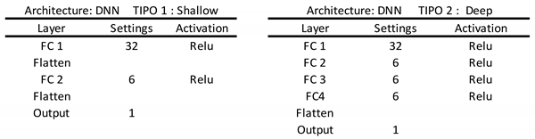 |
Table A2.
CNN model architecture.
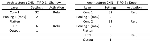 |
Table A3.
LSTM. model architecture.
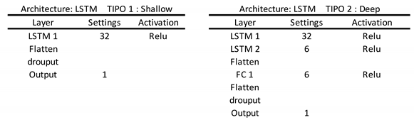 |
Table A4.
CNN+LSTM model architecture.
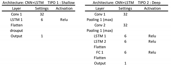 |
Appendix B. Hyperparameter Selection
Neural network models have internal parameters known as hyperparameters. Table B1 lists the main hyperparameters for the models. The last column contains the values obtained from the processes using the GridSearchCV function from Sklearn. These values were used in the experiments conducted in this study.
Table B1.
Hyperparameter Selection.
| Hyperparameter | Interval | Selection |
|---|---|---|
| Number of hidden layers | [1..100] | 1 to 6 |
| Number of neurons | [1..100] | 5 |
| Learning Rating | [0.0001..0.01] | 0.01 |
| Dropout rate | [0.1.. 0.5] | 0.1 |
| Activation function | Relu, Sigmoid, Tanh | Relu |
| Optimizer | Adam,RMSprop,SGD | Adam |
| Batch Size | [16..512] | 128 |
| Loss function | Mse, mae, mape | Mse |
| Kernel | [2..5] | 2 |
| Number of epochs | [10..500] | 30 |
References
- Merce, R.A.; Grover-Silva, E.; Le Conte, J. Load and Demand Side Flexibility Forecasting. In Proceedings of the ENERGY Tenth Int. Conf. Smart Grids, Green Commun. IT Energy-aware Technol, Lisbon, Portugal; 2020; pp. 1–6. [Google Scholar]
- Khan, K.A.; Quamar, M.M.; Al-Qahtani, F.H.; Asif, M.; Alqahtani, M.; Khalid, M. Smart Grid Infrastructure and Renewable Energy Deployment: A Conceptual Review of Saudi Arabia. Energy Strateg. Rev. 2023, 50, 101247. [Google Scholar] [CrossRef]
- Mystakidis, A.; Koukaras, P.; Tsalikidis, N.; Ioannidis, D.; Tjortjis, C. Energy Forecasting: A Comprehensive Review of Techniques and Technologies. Energies 2024, 17. [Google Scholar] [CrossRef]
- Peñaloza, A.K.A.; Balbinot, A.; Leborgne, R.C. Review of Deep Learning Application for Short-Term Household Load Forecasting. In Proceedings of the 2020 IEEE PES Transmission & Distribution Conference and Exhibition - Latin America (T&D LA); 2020; pp. 1–6. [Google Scholar]
- Aybar-Mejía, M.; Villanueva, J.; Mariano-Hernández, D.; Santos, F.; Molina-García, A. A Review of Low-Voltage Renewable Microgrids: Generation Forecasting and Demand-Side Management Strategies. Electronics 2021, 10. [Google Scholar] [CrossRef]
- Bunn, D.W. Short-Term Forecasting: A Review of Procedures in the Electricity Supply Industry. J. Oper. Res. Soc. 1982, 33, 533–545. [Google Scholar] [CrossRef]
- Min, H.; Hong, S.; Song, J.; Son, B.; Noh, B.; Moon, J. SolarFlux Predictor: A Novel Deep Learning Approach for Photovoltaic Power Forecasting in South Korea. Electronics 2024, 13. [Google Scholar] [CrossRef]
- Manzolini, G.; Fusco, A.; Gioffrè, D.; Matrone, S.; Ramaschi, R.; Saleptsis, M.; Simonetti, R.; Sobic, F.; Wood, M.J.; Ogliari, E.; et al. Impact of PV and EV Forecasting in the Operation of a Microgrid. Forecasting 2024, 6, 591–615. [Google Scholar] [CrossRef]
- Sengupta, S.; Basak, S.; Saikia, P.; Paul, S.; Tsalavoutis, V.; Atiah, F.; Ravi, V.; Peters, A. A Review of Deep Learning with Special Emphasis on Architectures, Applications and Recent Trends. Knowledge-Based Syst. 2020, 194, 105596. [Google Scholar] [CrossRef]
- Hahn, H.; Meyer-Nieberg, S.; Pickl, S. Electric Load Forecasting Methods: Tools for Decision Making. Eur. J. Oper. Res. 2009, 199, 902–907. [Google Scholar] [CrossRef]
- Park, H.-Y.; Lee, B.-H.; Son, J.-H.; Ahn, H.-S. A Comparison of Neural Network-Based Methods for Load Forecasting with Selected Input Candidates. In Proceedings of the 2017 IEEE International Conference on Industrial Technology (ICIT); 2017; pp. 1100–1105. [Google Scholar]
- Kong, W.; Dong, Z.Y.; Jia, Y.; Hill, D.J.; Xu, Y.; Zhang, Y. Short-Term Residential Load Forecasting Based on LSTM Recurrent Neural Network. IEEE Trans. Smart Grid 2019, 10, 841–851. [Google Scholar] [CrossRef]
- Mannini, R.; Darure, T.; Eynard, J.; Grieu, S. Predictive Energy Management of a Building-Integrated Microgrid: A Case Study. Energies 2024, 17. [Google Scholar] [CrossRef]
- Elsworth, S.; Güttel, S. Time Series Forecasting Using LSTM Networks: A Symbolic Approach 2020.
- Glavan, M.; Gradišar, D.; Moscariello, S.; Juričić, Đ.; Vrančić, D. Demand-Side Improvement of Short-Term Load Forecasting Using a Proactive Load Management – a Supermarket Use Case. Energy Build. 2019, 186, 186–194. [Google Scholar] [CrossRef]
- Alzubaidi, L.; Zhang, J.; Humaidi, A.J.; Al-Dujaili, A.; Duan, Y.; Al-Shamma, O.; Santamaría, J.; Fadhel, M.A.; Al-Amidie, M.; Farhan, L. Review of Deep Learning: Concepts, CNN Architectures, Challenges, Applications, Future Directions. J. Big Data 2021, 8, 53. [Google Scholar] [CrossRef] [PubMed]
- Ungureanu, S.; Topa, V.; Cziker, A.C. Deep Learning for Short-Term Load Forecasting—Industrial Consumer Case Study. Appl. Sci. 2021, 11. [Google Scholar] [CrossRef]
- Jiang, W. Deep Learning Based Short-Term Load Forecasting Incorporating Calendar and Weather Information. Internet Technol. Lett. 2022, 5, e383. [Google Scholar] [CrossRef]
- Alom, M.Z.; Taha, T.M.; Yakopcic, C.; Westberg, S.; Sidike, P.; Nasrin, M.S.; Hasan, M.; Van Essen, B.C.; Awwal, A.A.S.; Asari, V.K. A State-of-the-Art Survey on Deep Learning Theory and Architectures. Electronics 2019, 8. [Google Scholar] [CrossRef]
- Son, N. Comparison of the Deep Learning Performance for Short-Term Power Load Forecasting. Sustainability 2021, 13. [Google Scholar] [CrossRef]
- Rumelhart, D.E.; Hinton, G.E.; Williams, R.J. Learning Internal Representations by Error Propagation. In Parallel Distributed Processing: Explorations in the Microstructure of Cognition, {V}olume 1: {F}oundations; Rumelhart, D.E., Mcclelland, J.L., Eds.; MIT Press: Cambridge, MA, 1986; pp. 318–362. [Google Scholar]
- Parmezan, A.R.S.; Souza, V.M.A.; Batista, G.E.A.P.A. Evaluation of Statistical and Machine Learning Models for Time Series Prediction: Identifying the State-of-the-Art and the Best Conditions for the Use of Each Model. Inf. Sci. (Ny). 2019, 484, 302–337. [Google Scholar] [CrossRef]
- Yalcinoz, T.; Eminoglu, U. Short Term and Medium Term Power Distribution Load Forecasting by Neural Networks. Energy Convers. Manag. 2005, 46, 1393–1405. [Google Scholar] [CrossRef]
- Santos Amaral, L.; Medeiros de Araújo, G.; Reinaldo de Moraes, R.A. Analysis of the Factors That Influence the Performance of an Energy Demand Forecasting Model. Adv. Notes Inf. Sci. 2022, 2, 92–102. [Google Scholar] [CrossRef]
- Amaral, L.S.; de Araújo, G.M.; Moraes, R.; de Oliveira Villela, P.M. An Expanded Study of the Application of Deep Learning Models in Energy Consumption Prediction BT - Data and Information in Online Environments.; Pinto, A.L., Arencibia-Jorge, R., Eds.; Springer Nature Switzerland: Cham, 2022; pp. 150–162. [Google Scholar]
- Kuo, P.-H.; Huang, C.-J. A High Precision Artificial Neural Networks Model for Short-Term Energy Load Forecasting. Energies 2018, 11. [Google Scholar] [CrossRef]
- Dudek, G. Multilayer Perceptron for Short-Term Load Forecasting: From Global to Local Approach. Neural Comput. Appl. 2020, 32, 3695–3707. [Google Scholar] [CrossRef]
- Buildings. Available online: https://www.iea.org/energy-system/buildings.
- KawBamura, T. Distribution of Discomfort Index in Japan in Summer Season. J Meteorol. Res. 1965, 17, 460–466. [Google Scholar]
- Ono, H.-S.P.; Kawamura, T. Sensible Climates in Monsoon Asia. Int. J. Biometeorol. 1991, 35, 39–47. [Google Scholar] [CrossRef] [PubMed]
- Suganthi, L.; Samuel, A.A. Energy Models for Demand Forecasting—A Review. Renew. Sustain. Energy Rev. 2012, 16, 1223–1240. [Google Scholar] [CrossRef]
- Curry, B.; Morgan, P.H. Model Selection in Neural Networks: Some Difficulties. Eur. J. Oper. Res. 2006, 170, 567–577. [Google Scholar] [CrossRef]
- Zhang, G.; Eddy Patuwo, B.; Y. Hu, M. Forecasting with Artificial Neural Networks:: The State of the Art. Int. J. Forecast. 1998, 14, 35–62. [Google Scholar] [CrossRef]
- Petropoulos, F.; Apiletti, D.; Assimakopoulos, V.; Babai, M.Z.; Barrow, D.K.; Ben Taieb, S.; Bergmeir, C.; Bessa, R.J.; Bijak, J.; Boylan, J.E.; et al. Forecasting: Theory and Practice. Int. J. Forecast. 2022, 38, 705–871. [Google Scholar] [CrossRef]
- Cogollo, M.R.; Velasquez, J.D. Methodological Advances in Artificial Neural Networks for Time Series Forecasting. IEEE Lat. Am. Trans. 2014, 12, 764–771. [Google Scholar] [CrossRef]
- Lippmann, R. An Introduction to Computing with Neural Nets. IEEE ASSP Mag. 1987, 4, 4–22. [Google Scholar] [CrossRef]
- Sheela, K.G.; Deepa, S.N. Review on Methods to Fix Number of Hidden Neurons in Neural Networks. Math. Probl. Eng. 2013, 2013, 425740. [Google Scholar] [CrossRef]
- Chollet, F. Keras: The Python Deep Learning API. Available online: https://keras.io/.
- Ribeiro, A.M.N.C.; do Carmo, P.R.X.; Endo, P.T.; Rosati, P.; Lynn, T. Short- and Very Short-Term Firm-Level Load Forecasting for Warehouses: A Comparison of Machine Learning and Deep Learning Models. Energies 2022, 15. [Google Scholar] [CrossRef]
- Gnanambal, S.; Thangaraj, M.; Meenatchi, V.; Gayathri, V. Classification Algorithms with Attribute Selection: An Evaluation Study Using WEKA. Int. J. Adv. Netw. Appl 2018, 9, 3640–3644. [Google Scholar]
- Nespoli, A.; Ogliari, E.; Pretto, S.; Gavazzeni, M.; Vigani, S.; Paccanelli, F. Electrical Load Forecast by Means of LSTM: The Impact of Data Quality. Forecasting 2021, 3, 91–101. [Google Scholar] [CrossRef]
- Hobbs, B.F.; Helman, U.; Jitprapaikulsarn, S.; Konda, S.; Maratukulam, D. Artificial Neural Networks for Short-Term Energy Forecasting: Accuracy and Economic Value. Neurocomputing 1998, 23, 71–84. [Google Scholar] [CrossRef]
Figure 1.
Structure of a direct neural network.
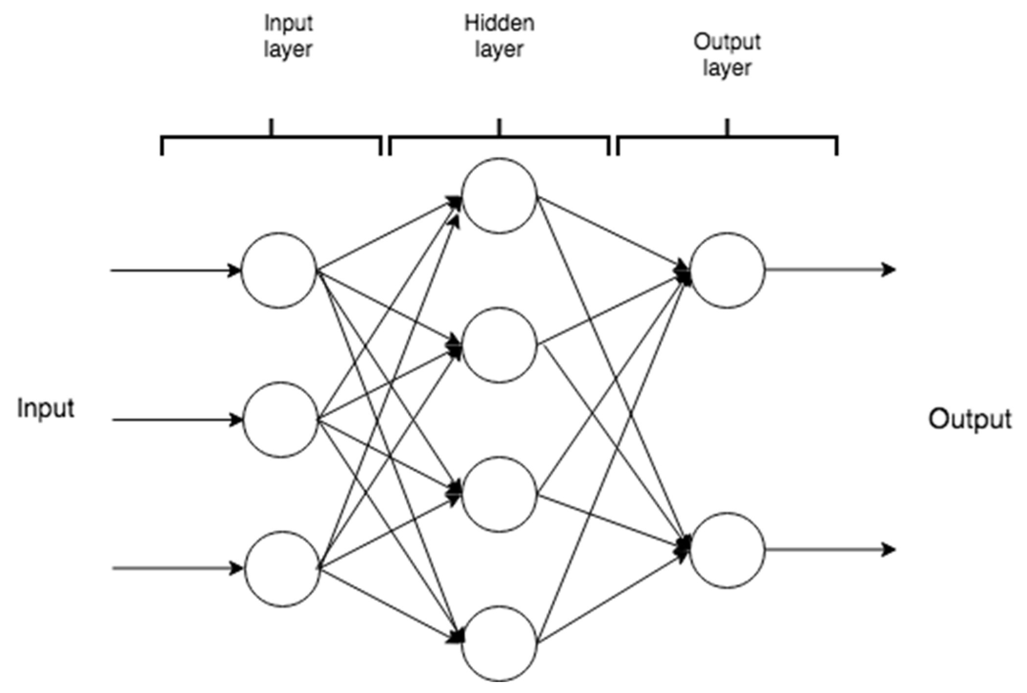
Figure 2.
Block diagram showing the training of a neural network.
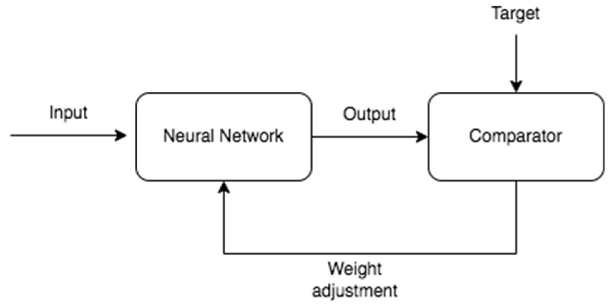
Figure 3.
LSTM Model Structure.
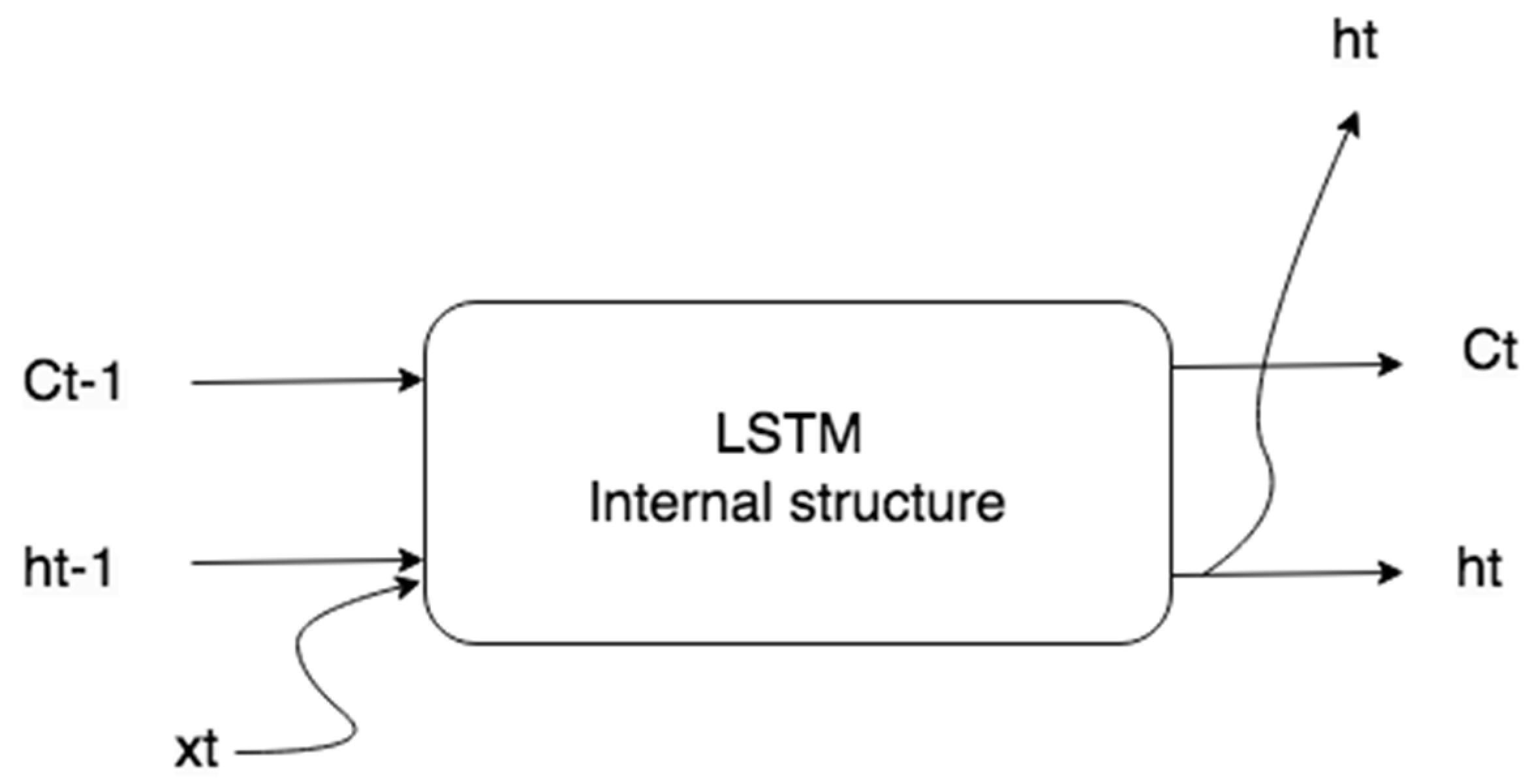
Figure 4.
Structure of a CNN model.
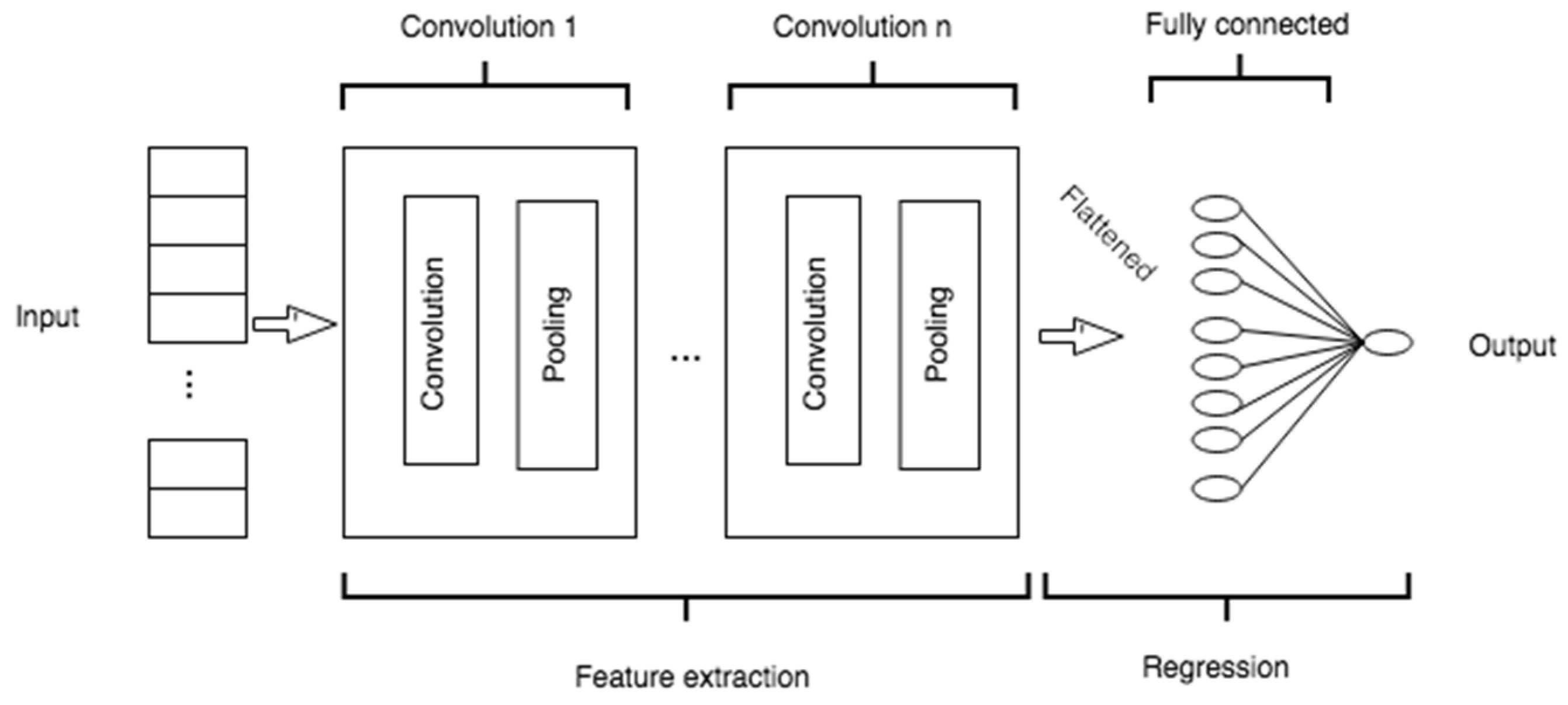
Figure 5.
Pipeline for creating an electricity consumption forecast model.
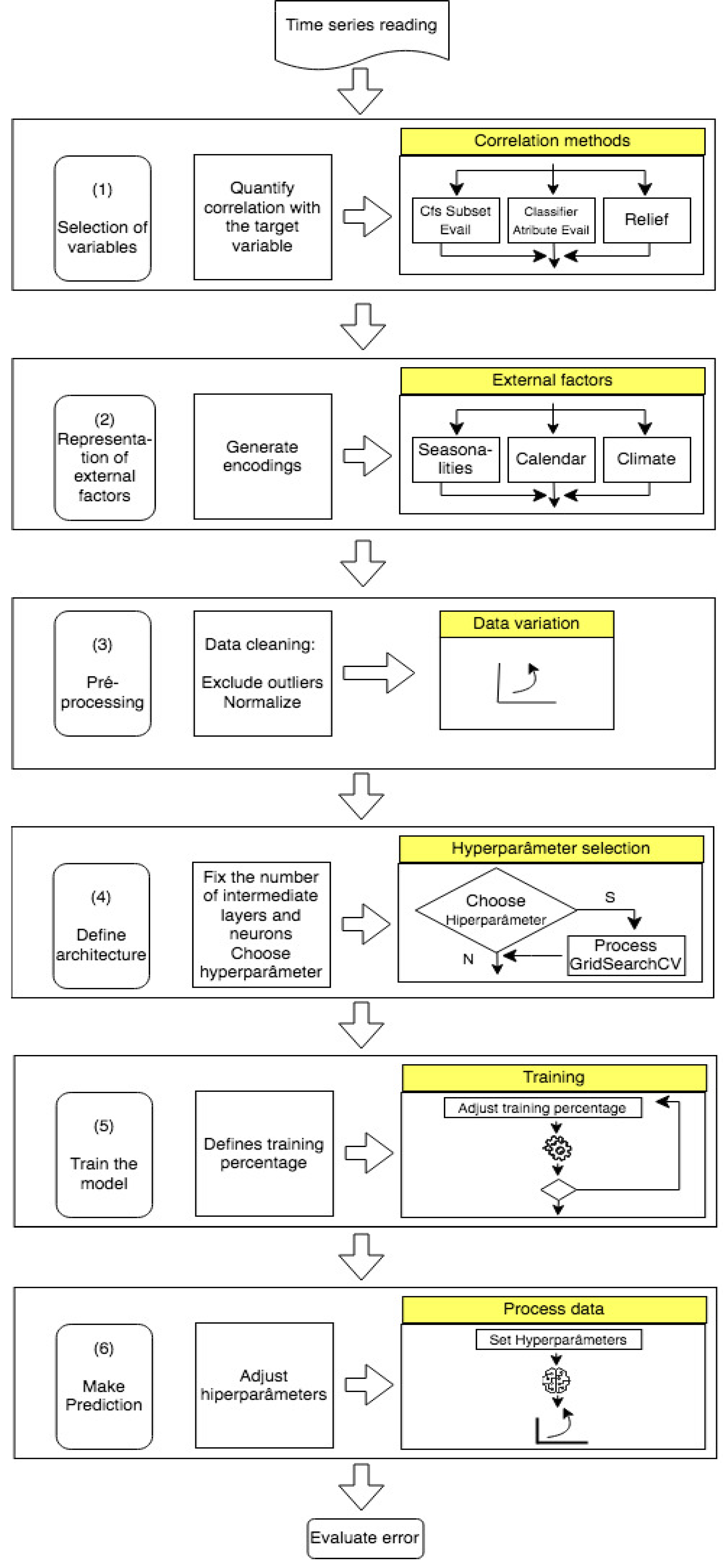
Figure 6.
Simulation detail flowchart.
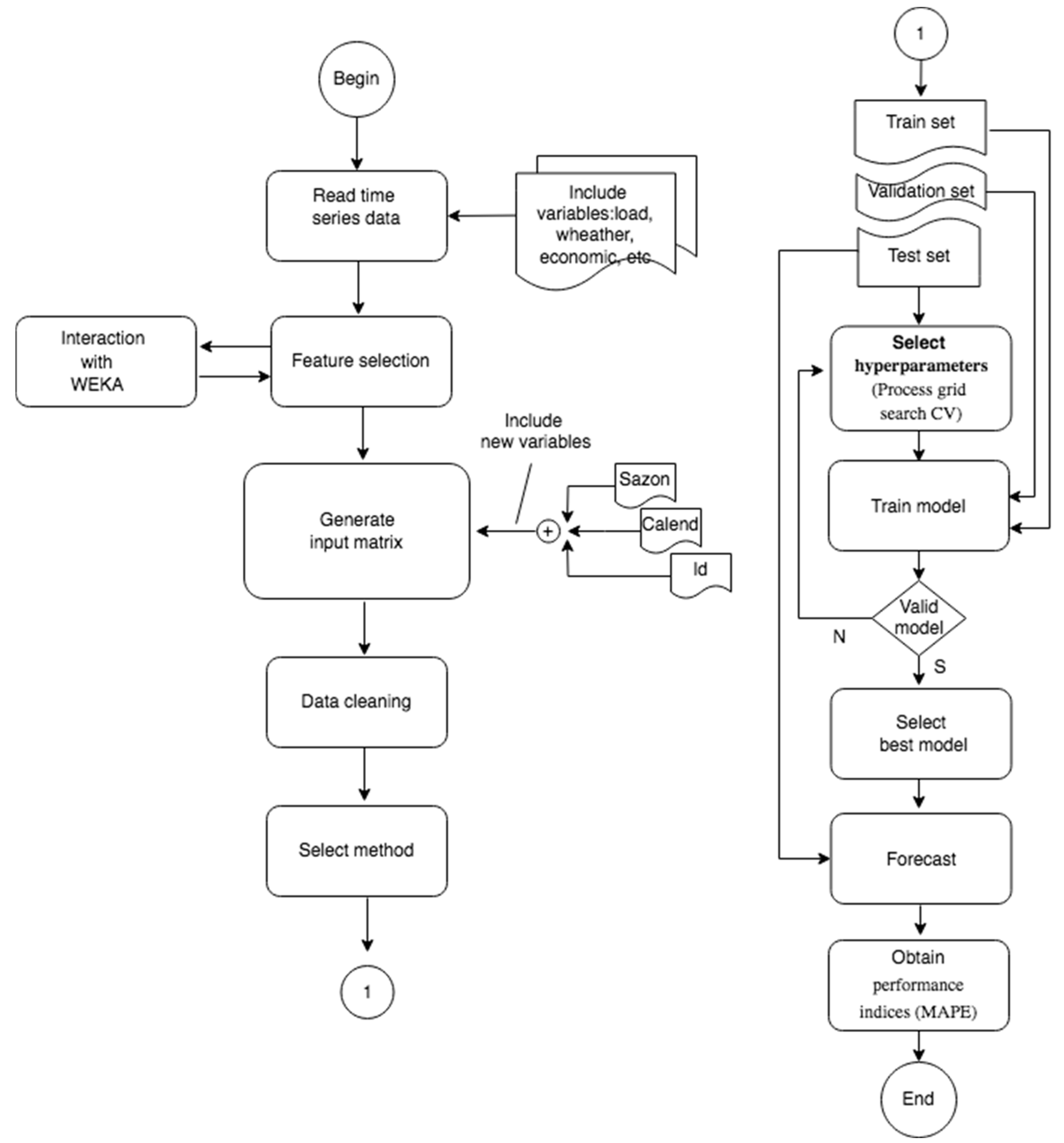
Figure 7.
Performance comparison of one-step-ahead predictors employing a shallow model.
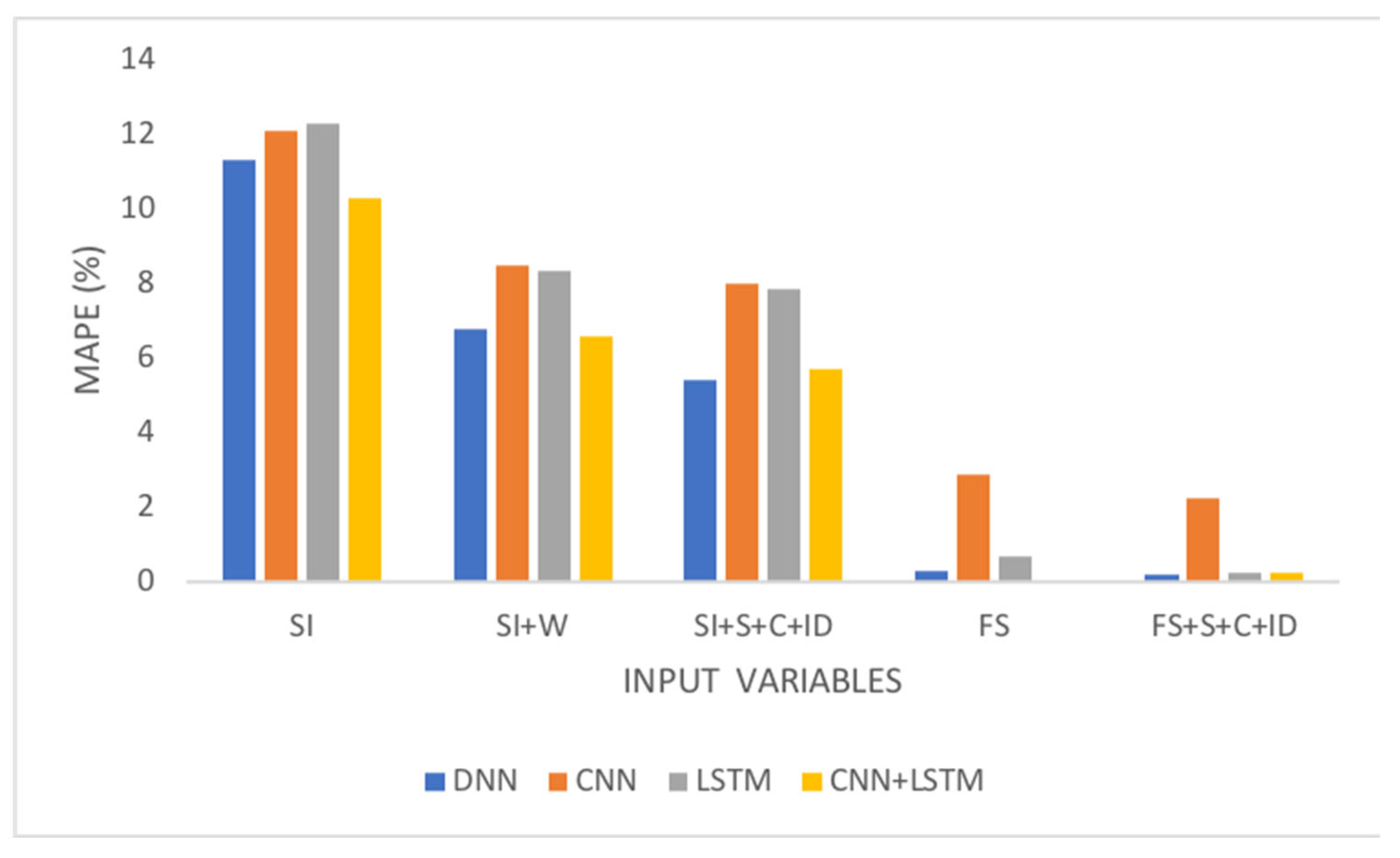
Figure 8.
Performance comparison of one-step-ahead predictors employing deep model.
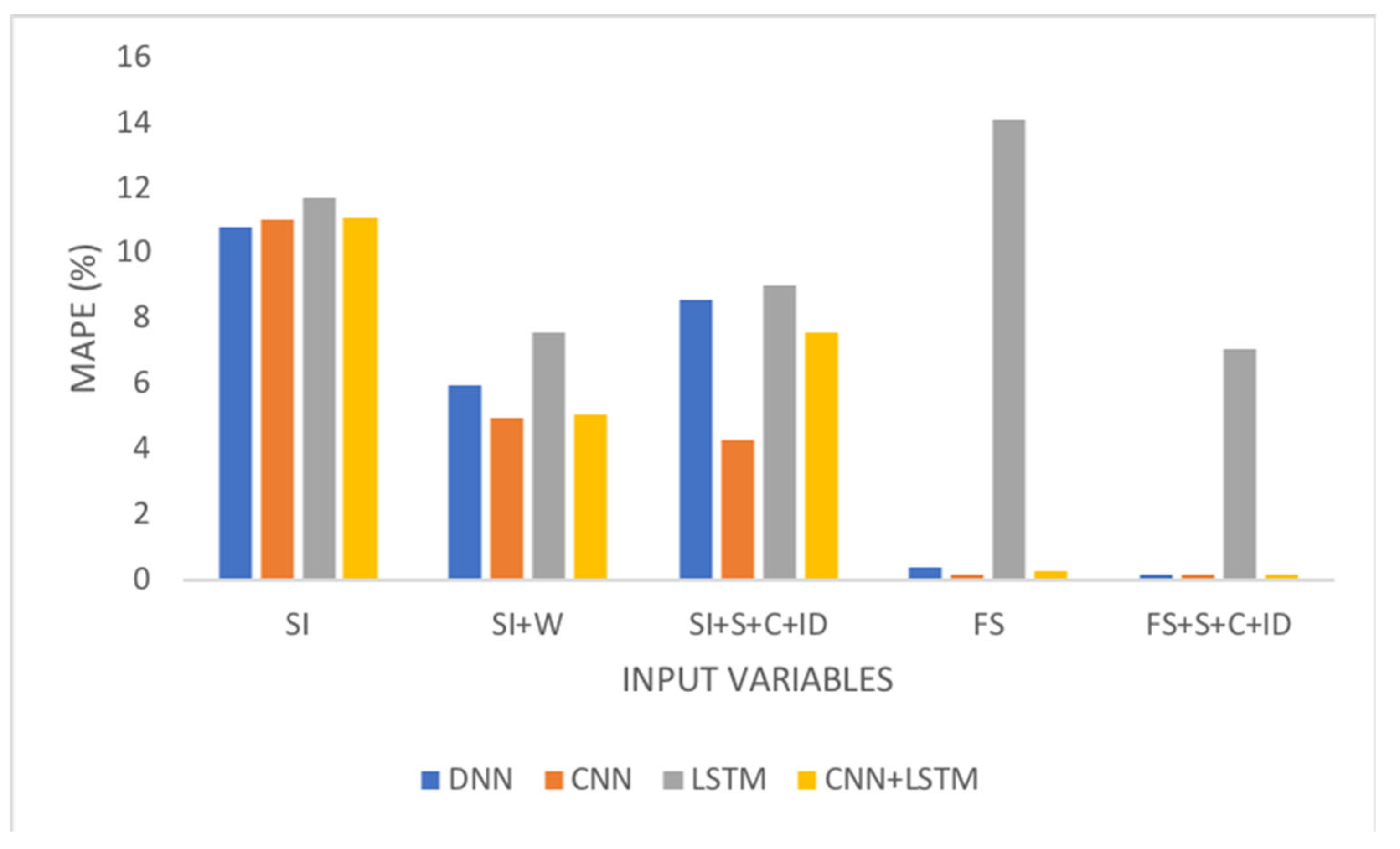
Figure 9.
Performance comparison of twelve-step-ahead predictors employing shallow model.
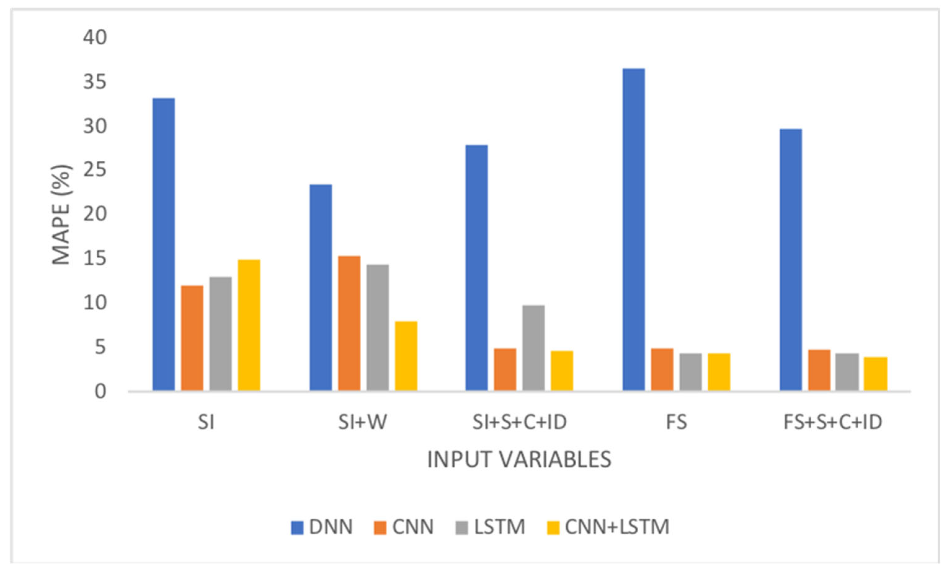
Figure 10.
Performance comparison of one-step-ahead predictors employing deep model.
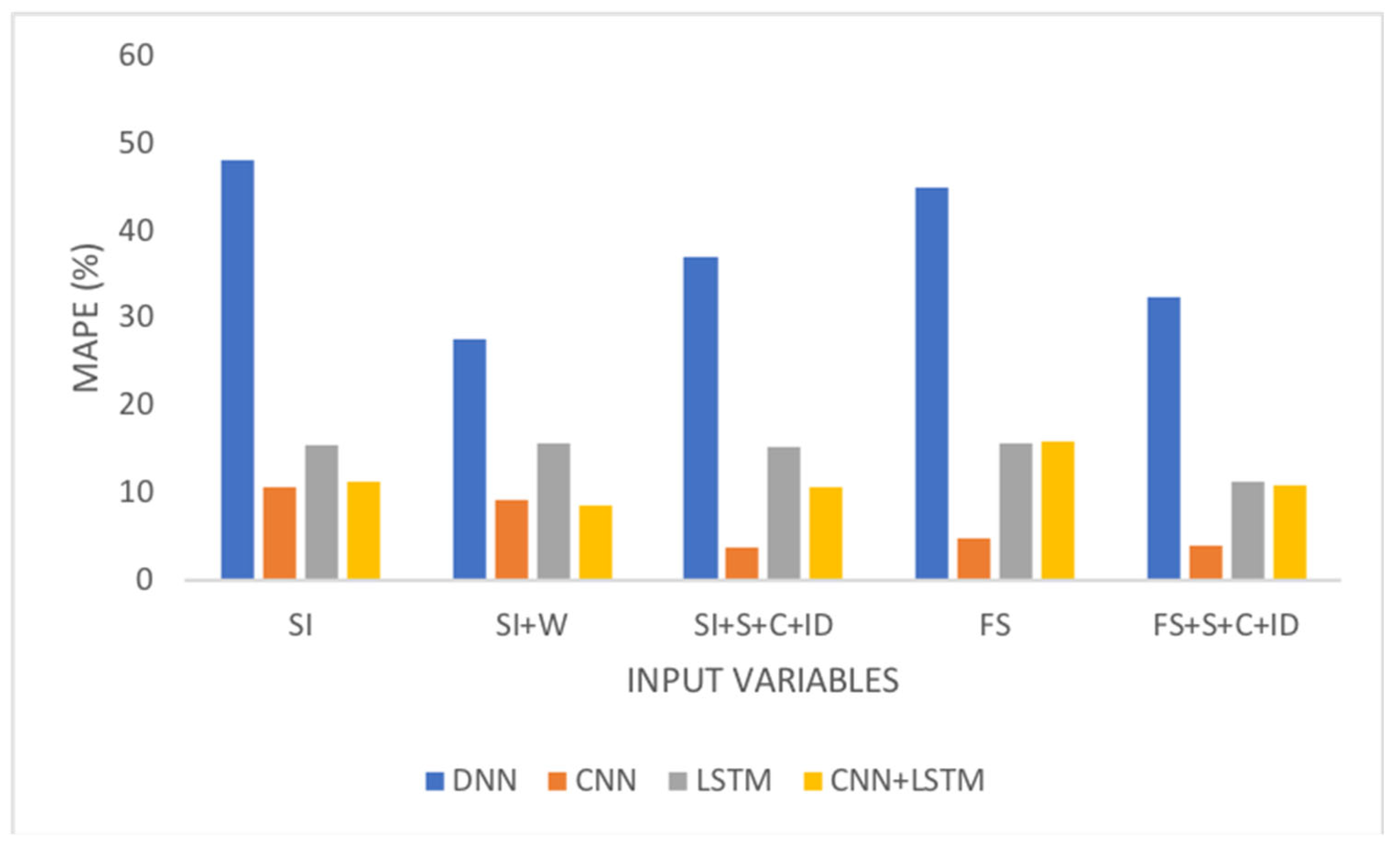
Table 1.
Temperature ranges for thermal comfort conditions.
| Interval | Condition |
|---|---|
| Id > 80 | Heat stress |
| 75 < Id < 80 | Uncomfortable due to heat |
| 60 < Id < 75 | Comfortable |
| 55 < Id < 60 | Uncomfortable due to cold |
| Id < 55 | Stress due to cold |
Table 2.
Encoding methods for date and time of day [18].
Table 2.
Encoding methods for date and time of day [18].
| Interval | Condition | Value Range |
|---|---|---|
| Holiday | Holiday or not | [0,1] |
| Workday | Workday or not | [0,0.5,1] |
| Working | Working or not | [0,0.5,1] |
Table 3.
Processes with variation in input variables (horizon: one step ahead).
| Technique |
Source | Selected variables |
Magnitude | DNN | CNN | LSTM | CNN+LSTM | ||||
|---|---|---|---|---|---|---|---|---|---|---|---|
| Shallow | Deep | Shallow | Deep | Shallow | Deep | Shallow | Deep | ||||
| CFS subset evaluation | WEKA |
RT demand, DACC, DA MLC, RT MLC, MIN_5MIN_RSP, MAX_5MIN_RSP |
MAPE | 0.22 | 0.18 | 1.8 | 0.74 | 0.37 | 0.24 | 0.21 | 0.18 |
| t(s) | 152 | 185 | 276 | 340 | 887 | 1798 | 739 | 848 | |||
|
Classifier attribute evaluation |
MAX_5MIN_RSP, DA EC, DA CC, RT demand, DA LMP | MAPE | 0.27 | 0.23 | 1.6 | 0.48 | 0.21 | 0.16 | 0.26 | 0.24 | |
| t(s) | 153 | 187 | 342 | 384 | 994 | 1813 | 761 | 790 | |||
| Principal components | RT LMP, RT EC, DA LMP, DA EC, RT MLC | MAPE | 7.8 | 6.84 | 9.67 | 6.5 | 10.95 | 9.79 | 8.06 | 7.57 | |
| t(s) | 87 | 130 | 150 | 219 | 594 | 912 | 996 | 386 | |||
| Relief | RT demand, DA demand, DA EC, DA LMC, reg. service price | MAPE | 0.52 | 0.33 | 3.82 | 0.22 | 0.23 | 0.16 | 0.16 | 0.17 | |
| t(s) | 112.8 | 123 | 274 | 339 | 906 | 1792 | 692 | 823 | |||
| Mutual information | Python | DA MLC, DA LMP, MIN_5MIN_RSP, DA EC, dew point | MAPE | 5.9 | 5.76 | 8.15 | 5.03 | 10.21 | 7.82 | 7.23 | 6.11 |
| t(s) | 155 | 186 | 270 | 339 | 581 | 1827 | 725 | 792 | |||
| - | - | All | MAPE | 0.86 | 0.38 | 2.27 | 1.05 | 0.29 | 0.2 | 0.25 | 0.20 |
| t(s) | 118 | 123 | 158 | 153 | 591 | 920 | 695 | 879 | |||
The best values are highlight in bold.
Table 4.
MAPE results for processes with different sets of input variables (horizon: one step ahead).
Table 4.
MAPE results for processes with different sets of input variables (horizon: one step ahead).
| Technique | Model | Sl (1) |
Sl+ W (2) |
Sl+ S+ C+ Id (3) |
(%) (4) |
Fs (5) |
Fs+ S+ C+ Id (6) |
(%) (7) |
Av (8) |
Av+ S+ C+ Id (9) |
(%) (10) |
|---|---|---|---|---|---|---|---|---|---|---|---|
| DNN | Sh | 11.3 | 6.76 | 5.38 | 52.4 | 0.29 | 0.19 | 34.5 | 0.19 | 0.18 | 5.3 |
| D | 10.85 | 5.98 | 8.57 | 44.9 | 0.37 | 0.17 | 54.1 | 0.22 | 0.17 | 22.7 | |
| CNN | Sh | 12.13 | 8.46 | 8.0 | 34 | 2.85 | 2.23 | 21.8 | 3.40 | 2.26 | 33.5 |
| D | 11.04 | 4.95 | 4.29 | 61.1 | 0.18 | 0.18 | 0 | 0.26 | 0.16 | 38.5 | |
| LSTM | Sh | 12.37 | 8.31 | 7.86 | 36.5 | 0.65 | 0.25 | 61.5 | 0.47 | 0.17 | 63.8 |
| D | 11.74 | 7.59 | 9.0 | 23.3 | 14.1 | 7.07 | 49.8 | 14.96 | 10.45 | 30.1 | |
| CNN+LSTM | Sh | 10.38 | 6.56 | 5.67 | 45.4 | 0.31 | 0.21 | 32.2 | 0.42 | 0.19 | 54.8 |
| D | 11.11 | 5.09 | 7.60 | 31.6 | 0.25 | 0.15 | 40 | 0.25 | 0.24 | 4 |
The best values are highlight in bold
Table 5.
MAPE results for processes with different sets of input variables (horizon: 12 steps ahead).
Table 5.
MAPE results for processes with different sets of input variables (horizon: 12 steps ahead).
| Technique | Model | Sl (1) |
Sl+ W (2) |
Sl+ S+ C+ Id (3) |
(%) (4) |
Fs (5) |
Fs+ S+ C+ Id (6) |
(%) (7) |
Av (8) |
Av+ S+ C+ Id (9) |
(%) (10) |
|---|---|---|---|---|---|---|---|---|---|---|---|
| DNN | Sh | 33.2 | 23.44 | 27.98 | 15.7 | 36.58 | 29.77 | 18.6 | 29.8 | 29.76 | 0.13 |
| D | 48.1 | 27.63 | 37.01 | 23.1 | 45.03 | 32.4 | 28.1 | 44.0 | 40.58 | 7.77 | |
| CNN | Sh | 12.01 | 15.37 | 4.92 | 59.0 | 4.91 | 4.83 | 1.6 | 4.92 | 4.68 | 4.9 |
| D | 10.6 | 9.19 | 3.77 | 64.4 | 4.79 | 3.96 | 17.3 | 4.39 | 3.63 | 17.7 | |
| LSTM | Sh | 13.00 | 14.36 | 9.82 | 24.5 | 4.39 | 4.30 | 2.0 | 4.29 | 3.66 | 14.7 |
| D | 15.58 | 15.65 | 15.27 | 2.0 | 15.8 | 11.34 | 4.46 | 15.4 | 15.15 | 1.62 | |
| CNN+LSTM | Sh | 15.00 | 8.04 | 4.58 | 69.5 | 4.42 | 3.93 | 11.0 | 4.12 | 4.09 | 0.7 |
| D | 11.24 | 8.65 | 10.7 | 4.8 | 15.94 | 10.82 | 32.1 | 15.6 | 15.36 | 1.5 |
The best values are highlight in bold
Table 6.
Simulation with deep models by varying the numbers of intermediate layers and neurons per intermediate layer.
Table 6.
Simulation with deep models by varying the numbers of intermediate layers and neurons per intermediate layer.
| DNN | CNN | LSTM | CNN+LSTM | ||||||||||
|---|---|---|---|---|---|---|---|---|---|---|---|---|---|
| Number of Neurons |
Number of neurons |
Number of neurons |
Number of neurons |
||||||||||
| 6 | 15 | 32 | 6 | 15 | 32 | 6 | 15 | 32 | 6 | 15 | 32 | ||
| Number of intermediate layers | 2 | 0.24 | 0.15 | 0.41 | 0.18 | 0.15 | 0.15 | 0.23 | 0.16 | 0.19 | 0.3 | 0.15 | 0.25 |
| 3 | 0.3 | 0.54 | 0.16 | 0.15 | 0.26 | 0.29 | 0.52 | 0.15 | 0.17 | 0.18 | 0.43 | 0.52 | |
| 4 | 0.17 | 0.44 | 0.2 | 0.19 | 0.18 | 0.17 | 2.34 | 0.46 | 0.81 | 0.18 | 0.17 | 0.17 | |
| 6 | 0.24 | 0.15 | 0.16 | 0.3 | 0.18 | 0.41 | 10.0 | 15.4 | 0.40 | 15.53 | 0.40 | 0.35 | |
The best values are highlight in bold
Disclaimer/Publisher’s Note: The statements, opinions and data contained in all publications are solely those of the individual author(s) and contributor(s) and not of MDPI and/or the editor(s). MDPI and/or the editor(s) disclaim responsibility for any injury to people or property resulting from any ideas, methods, instructions or products referred to in the content. |
© 2024 by the authors. Licensee MDPI, Basel, Switzerland. This article is an open access article distributed under the terms and conditions of the Creative Commons Attribution (CC BY) license (http://creativecommons.org/licenses/by/4.0/).
Copyright: This open access article is published under a Creative Commons CC BY 4.0 license, which permit the free download, distribution, and reuse, provided that the author and preprint are cited in any reuse.


