
Submitted:
08 July 2025
Posted:
09 July 2025
You are already at the latest version
Abstract
The growing demand for efficient energy management has become essential for achieving sustainable development across social, economic, and environmental sectors. Accurate energy demand forecasting plays a pivotal role in energy management. However, energy demand data presents unique challenges due to its complex characteristics, such as multi-seasonality, hidden structures, long-range dependency, irregularities, volatilities, and nonlinear patterns, making energy demand forecasting challenging. We propose a hybrid dimension reduction deep learning algorithm, Temporal Variational Residual Network (TVRN), to address these challenges and enhance forecasting performance. This model integrates Variational Autoencoders (VAEs), Residual Neural Networks (ResNets), and Bidirectional Long Short-Term Memory Networks (BiLSTM). TVRN employs VAEs for dimensionality reduction and noise filtering, ResNets to capture local, mid-level, and global features while tackling gradient vanishing issues in deeper networks, and BiLSTM to leverage past and future contexts for dynamic and accurate predictions. The performance of the proposed model is evaluated using energy consumption data, showing a significant improvement over traditional deep learning and hybrid models. For hourly forecasting, TVRN reduces root mean square error and mean absolute error, ranging from 19\% to 86\% compared to other models. Similarly, for daily energy consumption forecasting, this method outperforms existing models with an improvement in root mean square error and mean absolute error ranging from 30\% to 95\%. The proposed model significantly enhances the accuracy of energy demand forecasting by effectively addressing the complexities of multi-seasonality, hidden structures, and nonlinearity.
Keywords:
Bidirectional Long Short-Term Memory
; Energy Demand
; Forecasting
; Residual Neural Network
; ResNet
; Variational Autoencoder
1. Introduction
Energy is crucial for a nation’s economic growth, quality of life, and environmental sustainability. According to the U.S. Energy Information Administration, global energy consumption is projected to increase by 34% from 2022 to 2025, reaching 855 quadrillion BTUs [1]. Population growth and economic expansion have been the main drivers of increasing energy usage over the past decades [2]. Interestingly, AI-driven energy demand is expected to double by 2030 [3]. In response to this trend, many countries enforce energy codes and regulations to mitigate energy usage, promote energy efficiency, and reduce CO2 emissions [4]. Accurate energy demand forecasting is essential for sustainable resource allocation, informed policymaking, and minimizing waste, thereby ensuring economic stability and environmental sustainability [5].
Energy demand forecasting is typically structured across different time horizons, each serving distinct needs. The National Renewable Energy Laboratory (NREL) categorizes energy demand forecasting into short-term (e.g., minutes to several days), medium-term (e.g., a week to several months), and long-term (e.g., annual and beyond) predictions, which are defined as follows [7]. Short-term forecasting supports operational decisions, such as real-time grid management and handling demand fluctuations resulting from unexpected events. Medium-term forecasting is used for tactical planning, including maintenance scheduling, fuel procurement, and financial forecasting. Long-term forecasting is crucial in strategic decision-making, as it guides infrastructure investments, capacity expansion, and policy development. Each horizon employs different modeling approaches and addresses specific needs within the energy planning ecosystem. Since exogenous shocks influence tactical planning and strategic decision-making in energy demand time series, this study focuses on short-term energy demand (or consumption) forecasting to enhance operational efficiency and market responsiveness.
Energy demand forecasting has been extensively studied using various statistical and machine learning methods, including traditional ARIMA and its variants such as ARMAX, GARCH, ARX, and TARX [8,9,10,11,12], which serve as foundational tools due to their simplicity. However, these models are constrained by their inherent assumptions of linearity and stationarity, which limit their ability to model complex real-world energy demand behavior. Specifically, they struggle to capture nonlinear fluctuations, abrupt changes, and the presence of multiple overlapping seasonal cycles in energy consumption. To address these challenges, machine learning techniques such as Support Vector Machines (SVM) [13], Artificial Neural Networks (ANNs) [14], random forests [15], and gradient boosting [16] have been explored, improving forecast accuracy. While these techniques can capture nonlinearity and enhance forecasting accuracy, they typically rely on shallow architectures that struggle to model temporal dependencies and hierarchical time dynamics, particularly in long-term sequences. This restricts their capacity to grasp complex energy demand patterns, which involve multi-seasonality, hidden structures, long-range dependencies, and irregularities. Deep learning models, including Recurrent Neural Networks (RNN) [17], Convolutional Neural Networks (CNNs) [18], and Long Short-Term Memory networks (LSTM) [19], have demonstrated significant improvements by automatically extracting nonlinear features and modeling sequential dependencies. Nevertheless, these models are not without limitations: vanilla RNNs suffer from vanishing gradient issues; CNNs, while effective at capturing local spatial patterns, lack temporal awareness; and LSTMs, though more robust, can still struggle with multi-seasonality and long-term irregularities in volatile demand patterns. To enhance the forecasting performance beyond what standalone models can offer, numerous hybrid deep learning frameworks have been proposed in the domain of energy demand forecasting. These architectures aim to leverage the strengths of complementary models while mitigating individual limitations. Notably, hybrid models combining CNNs and recurrent architectures, such as CNN-LSTM [20], CNN-GRU [21], and attention-based CNN-LSTM-BiLSTM [22], have demonstrated promising results by integrating spatial and temporal representation learning. However, these models are not without their shortcomings. The CNN-LSTM architecture, for instance, often struggles with retaining long-term dependencies due to the LSTM’s limitations in memory when handling high-dimensional temporal and spatial inputs. Moreover, CNNs are generally optimized for grid-like image data and may not capture the nuanced temporal irregularities of energy usage without extensive preprocessing or customization [56]. Similarly, CNN-GRU hybrids, while computationally lighter than their LSTM counterparts, often underperform in tasks requiring fine-grained sequential learning, particularly when faced with multivariate and multi-seasonal energy data [57].
Dimensionality reduction (DR) techniques are increasingly integrated with deep learning to enhance energy demand forecasting, particularly for feature extraction and noise reduction. Traditional DR methods such as Principal Component Analysis (PCA) [23], Linear Discriminant Analysis (LDA), Singular Value Decomposition (SVD), and Non-Negative Matrix Factorization (NMF) [24] have been employed for preprocessing energy datasets before deep learning applications. To overcome the limitations of traditional DR techniques, autoencoders (AEs) and their variants, such as sparse autoencoders (SAEs) and variational autoencoders (VAEs), have been widely adopted. These unsupervised deep learning models leverage nonlinear transformations for feature extraction in deep neural networks [25,26,27,28]. SAEs introduce sparsity constraints to prevent overfitting and improve interpretability by selectively activating neurons. On the other hand, VAEs enhance traditional autoencoders by introducing a probabilistic framework where the encoder produces a distribution instead of a fixed vector and by including a Kullback-Leibler (KL) divergence term in the loss function. This enables generative modeling, smooth latent space interpolation, and greater robustness against overfitting [27,28]. These DR techniques have been combined with deep learning algorithms, e.g., complementary ensemble empirical mode decomposition with PCA and LSTM (CEEMD-PCA-LSTM) will be referred to as CPL [29], multilevel wavelet decomposition networks (MWDN) [30], variational mode decomposition (VMD) [31], and VAE-BiLSTM [32]. However, these methods often struggle to capture the complex low-dimensional structures inherent in energy data, partially due to their linear reduction. Furthermore, these methods struggle to capture local temporal patterns, seasonality, and long-term dependencies in energy data [33]. Addressing these challenges remains critical for advancing deep learning-based energy forecasting.
In deep learning model architectures such as Convolutional Neural Networks (CNNs) and VAEs, the depth of the hidden network layers, defined by the number of layers, plays a critical role in determining model performance. However, increasing the depth of the neural network often leads to a degradation problem, where the model’s accuracy decreases. Residual Neural Networks (ResNets), initially proposed for image analysis [34], address this issue by introducing a residual learning framework that facilitates the training of deep networks. ResNets achieve this by incorporating identity shortcut connections that bypass one or more layers, allowing gradients to propagate more effectively during backpropagation. These skip connections are implemented through residual blocks that perform element-wise addition between the input and output of convolutional layers. This mechanism addresses problems such as vanishing gradients, enabling the efficient training of deeper models. Furthermore, ResNets enhance the extraction of complex and abstract features by preserving historical information and reducing feature loss, allowing the model to learn more expressive and discriminative representations [34].
We propose a novel hybrid deep learning framework for dimensionality reduction, named the Temporal Variational Residual Network (TVRN), to address key challenges in energy demand, including multi-seasonality, hidden structures, long-range dependencies, and nonlinearity. By leveraging the strength of each component, TVRN aims to enhance energy demand forecasting. Our method begins with a ResNet embedded within a VAE, which enhances feature extraction at multiple levels, including the initial layers that detect local features such as short-term fluctuations, spikes, sudden changes, and irregularities. The intermediate layers capture seasonal and cyclical patterns. In contrast, the deeper layers identify global features, including long-term trends and notable correlation patterns in energy consumption data, by avoiding gradients vanishing, thereby improving forecasting performance [36]. VAEs, the encoder maps input data to a lower-dimensional latent space by generating a multivariate Gaussian distribution rather than a single point, thereby capturing a more robust and probabilistic latent representation [28]. BiLSTM enhances sequential analysis by incorporating bidirectional dependencies, leveraging past and future contexts for more accurate predictions. TVRN establishes a structured and efficient deep learning framework for energy demand forecasting by using hierarchical feature extraction, noise-filtered dimensionality reduction, and bidirectional sequential modeling. It offers a powerful approach to capturing complex temporal and structural patterns in energy data.
The contribution of this study is summarized as follows:
- We introduce an innovative dimensionality reduction-based hybrid deep learning framework algorithm that integrates a ResNet-embedded VAE with a BiLSTM architecture to improve feature extraction, uncover hidden patterns, and effectively address multi-seasonality and irregularities in energy consumption data.
- The hybrid forecasting model integrates ResNet-embedded VAEs with BiLSTM networks to improve forecasting accuracy. VAEs reduce dimensionality and denoise data, while ResNet addresses the vanishing gradient problem in deeper networks using skip connections, enabling efficient training and multi-scale feature extraction. BiLSTM further enhances performance by capturing temporal dependencies from past and future data.
- To the best of our knowledge, this work is the first to introduce a ResNet-embedded VAE for time series forecasting, leveraging ResNet’s ability, initially developed for image recognition, to enhance local, mid-term, and global feature extraction. At the same time, overcoming vanishing gradients in deep VAEs improves the accuracy of energy consumption forecasts.
- The proposed model, TVRN, is evaluated by comparing its performance against traditional models, such as ARIMA, as well as key deep learning architectures, including DNN, CNN, and BiLSTM, and hybrid solutions, including PCA-BiLSTM and CPL, with a particular emphasis on hourly and daily energy consumption data.
The remainder of this paper is organized as follows: Section 2 introduces the hybrid ResNet-embedded VAE-BiLSTM architecture. Section 3 outlines the experimental setup and details the hourly and daily energy consumption data used. Section 4 describes the result of the data analysis experiment. Section 5 provides a comprehensive discussion of the analytical results. Finally, Section 6 Conclusions presents the main findings.
2. Methodology
Consider a time series , which represents energy consumption recorded at regular intervals from time to T. This sequence exhibits multi-seasonality, hidden structures, nonlinearity, irregularity, and volatility. Section 2.1 presents a detailed exposition of the forecasting methodology and thoroughly elaborates on the architecture of the proposed model.
2.1. TVRN Algorithm Arichitecture
We present a novel approach to energy demand forecasting called TVRN, aimed at improving the accuracy of energy consumption predictions. The TVRN framework combines a ResNet-embedded VAE with a BiLSTM network to effectively model and learn patterns in energy demand, as depicted in Figure 1. The process begins with data preprocessing, which involves applying a logarithmic transformation and normalization to the energy demand data. Next, the ResNet-embedded VAE is utilized to analyze the preprocessed data. This step enables hierarchical multiscale feature extraction while performing dimensionality reduction and noise filtering, thereby addressing any degradation issues that may arise. The latent variables identified by the VAE capture the generative process of energy demand data, resulting in a more accurate representation of key temporal patterns. These latent representations are then sequentially processed by the BiLSTM, which models temporal dependencies by utilizing past and future information. Finally, the predicted output of the BiLSTM, which corresponds to the original energy demand values, is obtained through a denormalization process.
Consider energy demand data , is represented as follows:
Where f is a measurable function that can be either linear or nonlinear, and error meets the following criteria:
The autoregressive lag, p, will be determined through experimental trials of model training to effectively capture all past energy information. Before conducting the main analytical steps, we standardize the time series data described in (1). Standardization is favored over alternative scaling methods, such as min-max normalization, due to its effectiveness in enhancing model performance [37], improving numerical stability [38], and accelerating convergence [39].
2.2. ResNet-embedded VAE
The TVRN hybrid model’s ResNet encoder component, shown in Figure 1 and detailed in Figure 2, is embedded into the VAE (see Figure 3), processes input energy consumption according to (1), using residual blocks within the VAE. This configuration enables the extraction of complex hierarchical features while concurrently reducing dimensionality. ResNet initiates its hierarchical feature extraction with the initial layers, which detect local features such as short-term fluctuations, spikes, sudden changes, and irregularities. The intermediate layers capture seasonal and cyclical patterns, while the deeper layers identify global features, including long-term trends and notable correlation patterns in energy consumption data. This process utilizes residual blocks, skip connections, and stacked layers, as shown in Figure 2. For every residual block l in the TVRN ResNet encoder, the operation executed by each residual block [34] within the VAE encoder can be described as follows:
In this context, represents the input for the residual block, while denotes the complete set of weights and biases for that block. The function in (2) signifies the residual mapping, which transforms the data within the residual blocks. A residual block comprises several convolutional layers connected by a shortcut that combines the block’s input with its output, as shown in Figure 2. The ResNet component’s residual mapping includes a convolutional layer designed to extract local features [40], expressed as , where is the input, denotes the weight, and signifies the bias. The convolutional layer’s output undergoes Batch Normalization, standardizing the data values from a previous residual block, followed by an activation function that introduces nonlinearity. These processes are carried out sequentially within each residual block, repeated throughout all blocks until the final output is delivered, as illustrated in Figure 2. Expanding this for all residual blocks, in the VAE encoder, the output of the ResNet encoder in (2) after completing L residual blocks can be described as follows:
where represents the initial input.
The ResNet architecture enables the construction of deeper neural networks without encountering degradation issues, facilitating the hierarchical extraction of local, intermediate, and global features [34]. VAE encodes a given subsequence from (3) into a latent space representation, modeled as independent random variables z that follow a multivariate Gaussian distribution [35]. Unlike traditional Autoencoders, which generate deterministic embeddings, the VAE formulates latent variables as probabilistic entities, as illustrated in Figure 3. The latent variable z is governed by a prior distribution , allowing the model to learn a structured probabilistic manifold rather than a single-point estimate. The probabilistic nature of the VAE enables the estimation of the marginal likelihood function for reconstructing the observed data sequence , as detailed in [41]. The encoder network, denoted as , serves to approximate the intractable posterior distribution . Specifically, it learns to parameterize the mean and variance of a multivariate Gaussian distribution that best represents , facilitating efficient latent space encoding. Conversely, the decoder network, , reconstructs the original data sequence by learning the conditional distribution . This mapping from the latent space back to the data space ensures the generative capability of the VAE, allowing it to synthesize plausible reconstructions from the learned latent distribution.
The ResNet encoder in a ResNet-embedded VAE extracts features from and maps it to a multivariate Gaussian distribution in the latent space z and the posterior distribution of the latent space vector is given by [27,28]:
Where represents the approximate posterior distribution, denotes the ResNet encoder parameters (weights and biases), and and correspond to the mean and variance of the latent sample distribution, respectively. The latent space vector is computed as:
where represents the learnable parameters of the ResNet-embedded encoder.
A key challenge in training VAE comes from the stochastic nature of the latent space. The ResNet-based encoder generates a mean and variance from which latent representations are sampled. However, directly optimizing these sampled values using standard backpropagation is not feasible. To address this issue, VAEs utilize the reparameterization trick [27], which introduces a deterministic noise term modulated by the encoder’s learned parameters, facilitating gradient-based optimization. The latent space dimension is set to 8, and the corresponding latent variable, parameterized by the encoder’s mean and variance, is sampled as outlined in (5) becomes ,
where is sampled from a standard normal distribution.
The ResNet-based decoder network reconstructs the input by mapping the latent variables z back to the predicted data ,27,28] expressed as:
Where denotes the likelihood of the reconstructed data given the latent variables, represents the decoder parameters, and and are the reconstructed mean and variance, respectively. The latent representations of TVRN generated by a VAE can be more precisely controlled due to the variational lower bound used in its optimization. In a VAE framework, the objective is to maximize the Evidence Lower Bound (ELBO), which arises from the Kullback-Leibler (KL) divergence between the approximate posterior and the prior , along with the expected log-likelihood of the observed data [41]. To ensure stable training of the TVRN, the ELBO is maximized, formulated as [28]:
This objective ensures a balance between reconstruction accuracy and the regularization imposed by the latent space, fostering meaningful and structured representations of the input data. It comprises two key components: the expected log-likelihood term, quantifying reconstruction quality, and the KL divergence, which regularizes the latent space by aligning it with a standard Gaussian distribution.
2.3. Modeling a BiLSTM to capture energy demand dependencies using a latent space representation
Upon training the ResNet-embedded VAE in Section 2.2, synthetic training samples can be generated by sampling latent representations from the latent space and inputting them into the BiLSTM. The BiLSTM enhances information flow by incorporating forward and backward training mechanisms, leveraging bidirectional temporal dependencies for more effective sequence learning [42]. The trained BiLSTM, utilizing input from the latent space, is formulated as follows:
The training process of the BiLSTM is represented as , where denotes the set of learnable parameters governing both the forward and backward LSTM layers.
Table 1 illustrates the forward and backward processes, as shown in (8). BiLSTM captures long-range dependencies through the forward cell states , which process past patterns, and the backward cell state , which processes information from future time steps to the current cells [42]. This process is managed through BiLSTM components, including the input gate (i), forget gate (f), and output gate (o) equations for the forward LSTM, as provided in [43] and shown in Table 1.
The hidden states of the BILSTM network are obtained by concatenating the forward and backward hidden state vectors at every time step, which can be expressed as:
Generally, the TVRN algorithm for energy consumption data, which embeds ResNet into VAE and integrates with BiLSTM, is defined as:
Where are parameters specific to the ResNet-embedded VAE encoder and BiLSTM, respectively, learned during training. is original energy consumption time series data processed through the ResNet-embedded VAE encoder, latent space, and BiLSTM and the final output to obtain , the forecasting for the original energy consumption
Since the original data has been standardized, the final result from (10) is reverted to the original scale using anti-standardization: where is the sample standard deviation and is the sample mean.
2.4. Out-of-Sample Energy Demand Forecasting Using Recursive Algorithms and Evaluation Metrics
Once the TVRN is built and trained, as described in the methodology section, we apply it to forecast the test data. We adopt a recursive forecasting approach, where the trained model generates multi-step predictions using each forecasted value as an input for predicting the next step [44]. This iterative process enables the model to forecast all h future values at time t by leveraging previously predicted outputs [45]. On the other hand, direct multi-step forecasting predicts each time horizon independently, without relying on prior forecasted values, as demonstrated in [46]. The recursive multi-step forecasting approach relies on the trained model. At time t, the forecast for (where ) is iteratively generated through the recursive process:
As described in Figure 4, a critical aspect of the recursive forecasting process is using forecasted values as inputs when actual observations are unavailable at time t. For instance, the forecast is derived from the trained ’Model’ based on past observations . However, since the one-step ahead time series value is unknown at time t, it is replaced with its forecasted counterpart, . As the forecasting horizon h extends, the reliance on previously predicted values increases, potentially amplifying forecasting variance.
The final stage of model evaluation involves assessing its performance using various statistical metrics, including Mean Squared Error (MSE), Root Mean Squared Error (RMSE), and Mean Absolute Error (MAE). These metrics, which are influenced by the data scale, quantify the accuracy of predictions on test datasets. While there is no universal consensus regarding the optimal metric for forecasting evaluation, the Mean Squared Error (MSE) is frequently preferred due to its strong theoretical foundation in statistical modeling. MAE and MSE offer valuable insights into forecasting accuracy and the magnitude of prediction errors. However, MAE assigns equal weight to all errors, whereas MSE places greater emphasis on more significant errors, making it more sensitive to outliers [47]. This characteristic renders MSE particularly useful in scenarios where penalizing substantial deviations is crucial. The assessment metrics are expressed as follows.
where indicates the actual values while signifies the predicted values for both in-sample and out-of-sample forecasting. Furthermore, T refers to the total number of observations for either in-sample or out-of-sample data.
3. Data Descriptions
We analyzed hourly and daily power consumption data from PJM Interconnection LLC (PJM), a regional transmission organization (RTO) in the United States that oversees the electric transmission system across the Eastern region. The dataset spans 2002 to 2018 and contains 145,336 hourly and 6,057 daily records. The dataset is publicly available at . Figure 5 illustrates these complexities: strong seasonal trends with high variability and consumption spikes are evident in Figure 5a,c. The Hurst exponent (0.9109 for hourly, 0.8880 for daily) indicates persistence, while spectral entropy values (3.0579 for hourly, 4.0530 for daily) suggest significant noise. Autocorrelation functions (Figure 5b,d) show strong correlations across multiple lags with a sinusoidal pattern, reflecting seasonality. Squared coherence plots (Figure 5f,h) reveal a complex energy distribution across frequencies. Frequency domain analysis (Figure 5e,g) identifies dominant frequencies, with a primary 24-hour cycle (0.0417 Hz), intermediate 10-hour and 8-hour periodicities, and additional peaks at 0.1429 Hz (weekly cycle), 0.3 Hz, and 0.412 Hz (bi-daily fluctuations). These complex properties in energy demand underscore the need for advanced forecasting techniques.
We conduct the Augmented Dickey-Fuller (ADF) test [48] on both hourly and daily energy consumption data, reporting test statistics, p-values, and critical values at the 1%, 5%, and 10% significance levels. The analysis considers three regression specifications: ’c’ (constant), ’ct’ (constant and linear trend), and ’ctt’ (constant, linear, and quadratic trends). In all cases, the p-values are significantly below 0.05, firmly rejecting the null hypothesis of a unit root. Additionally, the KPSS test [49] does not reject the null hypothesis of stationarity, with a p-value (0.1 > 0.05), which reinforces that the data is stationary. A log transformation applied before model training offers key advantages: normalizing the data scale, mitigating outliers, and enhancing pattern recognition. Stabilizing variance is critical in energy data, where higher variability is observed at larger values, which supports models that usually assume distributed errors. Additionally, it simplifies modeling by converting multiplicative relationships into additive ones, improving the handling of seasonal variations in forecasting.
3.1. Design and Optimization of Hyperparameters
The dataset comprises 145,336 hourly energy consumption records, partitioned as follows: the first 145,012 hours for training, the next 300 hours for validation, and the final 24 hours for testing. The TVRN hybrid model was trained using optimized hyperparameters and demonstrated superior predictive performance. The optimal autoregressive order for hourly energy consumption is 96 hours. The latent space dimensionality is set to 8, with the encoder utilizing dense layers to compute the mean and log variance, followed by a sampling layer incorporating the Gaussian reparameterization trick. The BiLSTM component of the hybrid model consisted of multiple Bidirectional LSTM layers. The first layer contained 32 units with tanh activation and returning sequences, a dropout rate of 0.2, and batch normalization. Subsequent layers consisted of 16 and 8 units, respectively, employing kernel regularization with an L2 penalty of 0.0001. The fourth layer included four units with tanh activation, while the final output layer comprised a single unit with the same activation function. The TVRN model trains using a composite loss function that combines binary cross-entropy for reconstruction loss and KL divergence for regularization. The Adam optimizer minimizes the total loss using a batch size of 64 over 30 epochs, with the mean squared error (MSE) as the primary loss function. A comprehensive summary of the ResNet parameters used in the hybrid model is provided in Table 2. The entire model is implemented in Python. The ResNet-embedded VAE with BiLSTM is developed using the TensorFlow and Keras frameworks. Additionally, various machine learning and deep learning algorithms are utilized through the scikit-learn library.
4. Results
Based on the dataset described in Section 3 and the hyperparameter settings detailed in Section 3.1, we present the results summarized in Table 3 and Table 4, as well as Figure 6 and Figure 7.
Table 3 presents the performance metrics of the forecasting model for hourly energy consumption based on the in-sample data, along with three different out-of-sample forecasting horizons: h = 1 hour, 12 hours, and 24 hours. The results indicate that the proposed TVRN model consistently outperforms ARIMA, standard deep learning methods such as DNN, BiLSTM, and CNN, as well as hybrid models like CPL and PCA-BiLSTM across the selected forecasting horizons. For example, the TVRN hybrid model shows significant improvements in RMSE compared to PCA-BiLSTM by 86%, 48%, and 19%, and similarly, improvements compared to CPL are 99%, 41%, and 12% for h = 1 hour, 12 hours, and 24 hours, respectively. Improvements are also noted in the MAE metrics. The traditional ARIMA model performs worse than all other models for 12 and 24-hour forecasting horizons.
Figure 6 illustrates a visualization of different models forecasting hourly energy consumption compared to the actual observed values. Among these models, TVRN performs better in capturing trends in energy consumption. In contrast, the ARIMA model struggles with nonlinearity and is unable to represent energy consumption patterns accurately. Notably, the proposed model closely aligns with the actual values, indicating its effectiveness in capturing dependencies and temporal structures.
The total daily energy consumption data for 6057 days is divided into three parts: the first 5842 days for training, the next 200 days for validation, and the last 15 days for the test dataset. The hyperparameters used for model training are identical to those employed for training on hourly energy data, with an autoregressive order of 30.
Table 4 presents the performance metrics of the forecasting model for daily energy consumption, based on in-sample data, alongside three different out-of-sample forecasting horizons: h = 1 day, 7 days, and 15 days. The results show that the proposed TVRN hybrid model consistently outperforms ARIMA, standard deep learning methods, CPL, and PCA-BiLSTM across the selected forecasting horizons. For instance, the TVRN demonstrates a notable improvement in RMSE compared to PCA-BiLSTM by 95%, 35%, and 30%, and similarly, improvements compared to CPL are 92%, 61%, and 66% for h = 1 day, 7 days, and 15 days, respectively. Enhancements are also evident in the MAE metrics. The traditional ARIMA model performs worse for h = 7 and 15 days ahead of the forecast horizons.
Figure 7 compares daily energy consumption (represented by the blue line) with predictions made by different models. The ARIMA model (orange line) exhibits minimal fluctuations but struggles to respond to sudden changes. The DNN model (green line) captures some variations but consistently lags behind actual values. The CNN model (red line) responds to changes but often overestimates or underestimates its targets. The BiLSTM model (black line) closely aligns with actual trends, effectively capturing both peaks and troughs. The CPL model (brown line) produces a smoother curve but can sometimes deviate from the actual time series, indicating a smoothing effect. The PCA-BiLSTM model (cyan line) strikes a balance between dimensionality reduction and sequence modeling, while the TVRN model (purple line) effectively captures sharp changes and complex patterns. Both BiLSTM, PCA-BiLSTM, and TVRN (VAE-ResNet-BiLSTM) successfully track abrupt changes, whereas ARMA struggles with gradual trends. Among these, TVRN and BiLSTM demonstrate superior accuracy and adapt well to complex patterns, while CNN, CPL, and PCA-BiLSTM show varying degrees of deviation from the actual time series.
5. Discussion
We propose the TVRN, a hybrid deep learning framework based on dimension reduction that incorporates embedded dimension reduction for energy demand forecasting. This framework addresses the inherent challenges of forecasting energy consumption, including long-range dependencies, hidden structures, multi-seasonality, and nonlinear behaviors. Empirical studies demonstrate that the proposed TVRN model consistently outperforms traditional statistical models, standard deep learning approaches, and existing hybrid models regarding RMSE and MAE. We evaluated TVRN on hourly and daily energy consumption data, comparing its predictive accuracy across multiple forecasting horizons against various benchmark models, as presented in Table 3 and Table 4. The results indicate that TVRN achieves superior forecasting accuracy compared to traditional models, such as ARIMA, deep learning models, including DNN, BiLSTM, and CNN, and hybrid models, including PCA-BiLSTM and CPL. For instance, for hourly forecasting, the hybrid TVRN model reduces root mean square error and mean absolute error, ranging from 19% to 86% compared to to other models. Similarly, for daily energy consumption forecasting, it outperforms existing models with an improvement in root mean square error and mean absolute error ranging from 30% to 95%. Additionally, the forecasting plots for hourly and daily energy consumption, presented in Figure 6 and Figure 7, demonstrate that TVRN effectively maintains close forecasting performance across energy data studies. In contrast, alternative models, such as ARIMA and CPL, exhibit deviations from actual values, as shown in Figure 7.
The superior performance of the proposed TVRN architecture can be attributed to several key factors. First, VAEs, as a class of deep generative models, learn latent representations of energy consumption instead of directly modeling raw data, which enhances forecasting accuracy [50]. By capturing the underlying generative energy consumption data process through latent random variables, VAEs facilitate a more precise representation of essential temporal patterns in time series data [51]. Second, integrating ResNet into the VAE framework significantly enhances the encoder’s feature extraction capability, resulting in a more informative representation of the latent space. In TVRN, ResNet plays a pivotal role in mitigating the vanishing gradient problem through skip connections while enhancing the learning of residual representations. This architecture enables effective multi-scale feature extraction, capturing local patterns such as short-term fluctuations and abrupt changes, intermediate structures such as seasonal and cyclic variations, and global trends characterized by long-range dependencies. ResNet improves stability and efficiency in feature learning by preserving gradient flow in deep networks, thereby increasing the model’s capacity to extract hierarchical temporal dependencies and enhancing predictive accuracy in complex time series forecasting. This integration between VAE’s generative modeling and ResNet’s hierarchical feature extraction reinforces the model’s superior forecasting performance.
Our findings highlight the advantages of a hybrid dimension reduction-based deep learning framework over single deep learning models, emphasizing the importance of dimension reduction through multilevel feature extraction using ResNet, as described in reference [52]. This study further confirms the effectiveness of hybrid deep learning approaches over single-model architectures, as supported by the existing literature [53,54]. This discovery reinforces the benefits of hybrid frameworks in capturing complex temporal dependencies, thereby improving the accuracy of energy demand forecasting. The latent vector derived from the ResNet encoder follows a multi-Gaussian distribution, playing a vital role in hierarchical feature extraction. This facilitates a flexible and probabilistic representation of latent space, effectively capturing the intricate and nonlinear characteristics of energy consumption data capabilities that PCA-based methods and VAE alone lack.
PCA-based hybrid models, such as PCA-BiLSTM and CPL [55], utilize linear transformations for dimensionality reduction. However, these models struggle to capture the complex patterns inherent in energy consumption data. While PCA-BiLSTM outperforms single deep learning models at h = 1 hour, CPL shows superior performance at h = 1 day ahead forecasting. However, both models exhibit significant underperformance compared to single deep-learning models at longer-term forecasting horizons. Specifically, in the hourly energy consumption study, PCA-based models perform poorly for h = 12 and h = 24 hours. In the daily energy study, they underperform for h = 7 and h = 15 days, as shown in Table 3 and Table 4. These findings suggest that PCA-based hybrid models are insufficient for capturing the intricate dynamics of energy consumption forecasting. In contrast, the TVRN model consistently delivers superior forecasting performance across empirical studies of energy consumption, as shown in Section 3. This improvement can be attributed to ResNet’s ability to extract local, intermediate, and global features, thereby effectively capturing the inherent complexities of energy consumption data, including multi-seasonality, long-range dependencies, nonlinearity, and hidden structures.
Although our proposed hybrid model demonstrates promising improvements in forecasting energy consumption, the TVRN model has certain limitations. First, this study does not account for forecasting intervals despite its superior performance. Second, the constraints imposed on the VAE latent space by the multivariate Gaussian distribution. Moreover, our model outperformed other approaches in terms of root mean squared error (RMSE) and mean absolute error (MAE) in both cases. However, some segments of the hourly forecast visualizations in Figure 6 exhibit flat, straight-line predictions. This behavior may be attributed possible factors: (1) the VAE may have learned a latent representation with limited variation or dynamic range in those intervals, resulting in nearly identical outputs, and (2) due to the recursive forecasting approach where predicted values are fed back as inputs early-stage errors or latent space saturation could propagate, leading to a sequence of flat predictions.
6. Conclusions
In this paper, we develop an innovative hybrid model called TVRN to address the challenges inherent in energy demand data, including multi-seasonality, hidden structures, irregular patterns, and nonlinearity. The proposed hybrid model integrates a VAE for dimensionality reduction, local feature extraction, and noise filtering. Simultaneously, the ResNet embedded within the VAE captures local, intermediate, and global features at shallow, mid-level, and deep levels, thereby addressing the vanishing gradient problem that often occurs in deeper networks. The BiLSTM component, on the other hand, captures sequential information through forward and backward propagation. Through the analysis of hourly and daily energy consumption, the results demonstrate that TVRN outperforms ARIMA, deep learning models (DNN, BiLSTM, CNN), and hybrid models (PCA-BiLSTM, CPL) in out-of-sample forecasting, achieving better accuracy in both RMSE and MAE. Our findings indicate that TVRN, which embeds a ResNet architecture into a variational autoencoder, demonstrates significant potential to improve the accuracy of energy consumption forecasting, particularly in capturing nonlinear patterns and complex seasonal structures in temporal dynamics.
Future research on TVRN could extend its capabilities by exploring alternative latent space distributions beyond the standard multivariate Gaussian assumption, thereby enhancing representation learning. Furthermore, investigating techniques for quantifying forecasting uncertainty, such as constructing prediction intervals, may improve the hybrid TVRN model’s robustness and reliability.
Author Contributions
Conceptualization, Simachew Ashebir and Seongtae Kim; methodology, S.A.; software, S.A.; validation, S.A., and S.K.; formal analysis, S.A.; investigation, S.A.; resources, S.A. and S.K.; data curation, S.A.; writing-original draft preparation, S.A.; writing-review and editing, S.K.; visualization, S.A.; supervision, S.K.; project administration, S.A.; funding acquisition, S.K. All authors have read and agreed to the published version of the manuscript.
Funding
This work was partly supported by the Alfred P. Sloan Foundation Grant #G-2020-1392 and NSF DMS-EiR Grant #2100729.
Data Availability Statement
The dataset is publicly available at https://www.kaggle.com/datasets/robikscube/hourly-energy-consumption?select=PJME_hourly.csv
Acknowledgments
During the preparation of this manuscript/study, the author(s) used ChatGPT 4o and Grammarly to edit and enhance the grammar of the manuscript. The authors have reviewed and edited the output and take full responsibility for the content of this publication.
Conflicts of Interest
The authors declare that there is no conflict of interest regarding the publication of this paper.
Abbreviations
The following abbreviations are used in this manuscript:
| TVRN | TEMPORAL VARIATIONAL RESIDUAL NETWORK |
| ARIMA | Autoregressive integrated moving average |
| ARMAX | AutoRegressive Moving Average with eXogenous |
| GARCH | Generalized AutoRegressive Conditional Heteroskedasticity |
| ARX | AutoRegressive with eXtra input |
| TARX | Threshold AutoRegressive with eXogenous |
| SVM | Support Vector Machines |
| ANNs | Artificial Neural Networks |
| RNN | Recurrent Neural NEtwork |
| CNNs | Convolutional Neural Networks |
| LSTM | Long Short Term Memory |
| BiLSTM | Bidirectional Long Short Term Memory |
| GRU | Gated Recurrent Unit |
| PCA | Principal Component Analysis |
| CEEMD | complementary ensemble empirical 81 mode decomposition |
| AE | Autoencoder |
| VAE | Varational Autoencoder |
| MWDN | Multilevel wavelet decomposition networks |
| (SVD) | Singular Value Decomposition |
References
- U.S. Energy Information Administration (2023), International Energy Outlook 2023.
- Suganthi, L., & Samuel, A. A. (2012). Energy models for demand forecasting—A review. Renewable and sustainable energy reviews, 16(2), 1223-1240.
- Chen, S. (2025). Data centres will use twice as much energy by 2030-driven by AI. Nature. [CrossRef]
- Zhao, H. X., & Magoulès, F. (2012). A review on the prediction of building energy consumption. Renewable and Sustainable Energy Reviews, 16(6), 3586-3592. [CrossRef]
- Wei, N., Li, C., Peng, X., Zeng, F., & Lu, X. (2019). Conventional models and artificial intelligence-based models for energy consumption forecasting: A review. Journal of Petroleum Science and Engineering, 181, 106187. [CrossRef]
- Klyuev, R. V., Morgoev, I. D., Morgoeva, A. D., Gavrina, O. A., Martyushev, N. V., Efremenkov, E. A., & Mengxu, Q. (2022). Methods of forecasting electric energy consumption: A literature review. Energies, 15(23), 8919. [CrossRef]
- National Renewable Energy Laboratory. (2022). Best practices in electricity load modeling and forecasting for long-term power sector planning (NREL/TP-6A20-81897). U.S. Department of Energy.
- Cuaresma, J. C., Hlouskova, J., Kossmeier, S., & Obersteiner, M. (2004). Forecasting electricity spot-prices using linear univariate time-series models. Applied Energy, 77(1), 87-106. [CrossRef]
- Bakhat, M., & Rosselló, J. (2011). Estimation of tourism-induced electricity consumption: The case study of the Balearic Islands, Spain. Energy economics, 33(3), 437-444. [CrossRef]
- Garcia, R. C., Contreras, J., Van Akkeren, M., & Garcia, J. B. C. (2005). A GARCH forecasting model to predict day-ahead electricity prices. IEEE transactions on power systems, 20(2), 867-874. [CrossRef]
- Moghram, I., & Rahman, S. (1989). Analysis and evaluation of five short-term load forecasting techniques. IEEE Transactions on Power Systems, 4(4), 1484-1491. [CrossRef]
- Weron, R., & Misiorek, A. (2008). Forecasting spot electricity prices: A comparison of parametric and semiparametric time series models. International journal of forecasting, 24(4), 744-763. [CrossRef]
- Dong, B., Cao, C., & Lee, S. E. (2005). Applying support vector machines to predict building energy consumption in tropical region. Energy and Buildings, 37(5), 545-553. [CrossRef]
- Rodrigues, F., Cardeira, C., & Calado, J. M. F. (2014). The daily and hourly energy consumption and load forecasting using artificial neural network method: a case study using a set of 93 households in Portugal. Energy Procedia, 62, 220-229. [CrossRef]
- Lahouar, A., & Slama, J. B. H. (2015). Day-ahead load forecast using random forest and expert input selection. Energy Conversion and Management, 103, 1040-1051. [CrossRef]
- Taieb, S. B., & Hyndman, R. J. (2014). A gradient boosting approach to the Kaggle load forecasting competition. International journal of forecasting, 30(2), 382-394.
- Shi, H., Xu, M., & Li, R. (2017). Deep learning for household load forecasting—A novel pooling deep RNN. IEEE Transactions on Smart Grid, 9(5), 5271-5280. [CrossRef]
- Wang, H. Z., Li, G. Q., Wang, G. B., Peng, J. C., Jiang, H., & Liu, Y. T. (2017). Deep Learning-Based Ensemble Approach for Probabilistic Wind Power Forecasting. Applied Energy, 188, 56-70. [CrossRef]
- Bedi, J., & Toshniwal, D. (2019). Deep Learning Framework for Forecasting Electricity Demand. Applied energy, 238, 1312-1326. [CrossRef]
- Kim, T. Y., & Cho, S. B. (2019). Predicting residential energy consumption using CNN-LSTM neural networks. Energy, 182, 72-81. [CrossRef]
- Xuan, W., Shouxiang, W., Qianyu, Z., Shaomin, W., & Liwei, F. (2021). A multi-energy load prediction model based on deep multi-task learning and an ensemble approach for regional integrated energy systems. International Journal of Electrical Power & Energy Systems, 126, 106583. [CrossRef]
- Wu, K., Wu, J., Feng, L., Yang, B., Liang, R., Yang, S., & Zhao, R. (2021). An attention-based CNN-LSTM-BiLSTM model for short-term electric load forecasting in an integrated energy system. International Transactions on Electrical Energy Systems, 31(1), e12637.
- Maćkiewicz, A., & Ratajczak, W. (1993). Principal components analysis (PCA). Computers & Geosciences, 19(3), 303-342.
- Lee, D., & Seung, H. S. (2000). Algorithms for non-negative matrix factorization. Advances in Neural Information Processing Systems, 13.
- Hinton, G. E., & Salakhutdinov, R. R. (2006). Reducing data dimensionality with neural networks. science, 313(5786), 504-507.
- Ng, A. (2011). Sparse autoencoder. CS294A Lecture notes, 72(2011), 1-19.
- Kingma, D. P., & Welling, M. (2013, December). Auto-encoding variational bayes.
- Kingma, D. P., & Welling, M. (2019). An introduction to variational autoencoders. Foundations and Trends® in Machine Learning, 12(4), 307-392.
- Zhang, Y. A., Yan, B., & Aasma, M. (2020). A novel deep learning framework: Prediction and analysis of finanEmpirical Mode Decomposition: A Noise-Assisted Data Analysis Methodions, 159, 113609.
- Wang, J., Wang, Z., Li, J., & Wu, J. (2018, July). Multilevel Wavelet Decomposition Network for Interpretable Time Series Analysis. In Proceedings of the 24th ACM SIGKDD international conference on knowledge discovery & data mining (pp. 2437-2446).
- Dragomiretskiy, K., & Zosso, D. (2013). Variational mode decomposition. IEEE Transactions on Signal Processing, 62(3), 531-544.
- Kim, T., Lee, D., & Hwangbo, S. (2024). A deep-learning framework for forecasting renewable demands using variational auto-encoder and bidirectional long short-term memory. Sustainable Energy, Grids and Networks, 38, 101245. [CrossRef]
- Cai, B., Yang, S., Gao, L., & Xiang, Y. (2023). Hybrid variational autoencoder for time series forecasting. Knowledge-Based Systems, 281, 111079. [CrossRef]
- He, K., Zhang, X., Ren, S., & Sun, J. (2016). Deep residual learning for image recognition. In Proceedings of the IEEE conference on computer vision and pattern recognition (pp. 770-778).
- Kingma, D. P., & Welling, M. (2013, December). Auto-encoding variational bayes.
- Chen, K., Chen, K., Wang, Q., He, Z., Hu, J., & He, J. (2018). Short-term load forecasting with deep residual networks. IEEE Transactions on Smart Grid, 10(4), 3943-3952. [CrossRef]
- Orr, G. B., & Müller, K. R. (Eds.). (1998). Neural networks: tricks of the trade. Berlin, Heidelberg: Springer Berlin Heidelberg.
- Goodfellow, I., Bengio, Y., Courville, A., & Bengio, Y. (2016). Deep learning (Vol. 1, No. 2). Cambridge: MIT press.
- Ioffe, S., & Szegedy, C. (2015, June). Batch normalization: Accelerating deep network training by reducing internal covariate shift. In International conference on machine learning (pp. 448-456). pmlr.
- Li, Z., Liu, F., Yang, W., Peng, S., & Zhou, J. (2021). A survey of convolutional neural networks: analysis, applications, and prospects. IEEE transactions on neural networks and learning systems, 33(12), 6999-7019.
- Doersch, C. (2016). Tutorial on variational autoencoders. arXiv preprint arXiv:1606.05908.
- Siami-Namini, S., Tavakoli, N., & Namin, A. S. (2019, December). The performance of LSTM and BiLSTM in forecasting time series. In 2019 IEEE International conference on big data (Big Data) (pp. 3285-3292). IEEE.
- Hochreiter, S., & Schmidhuber, J. (1997). Long short-term memory. Neural computation, 9(8), 1735-1780.
- Cheng, H., Tan, P. N., Gao, J., & Scripps, J. (2006). Multistep-ahead time series prediction. In Advances in Knowledge Discovery and Data Mining: 10th Pacific-Asia Conference, PAKDD 2006, Singapore, April 9-12, 2006. Proceedings 10 (pp. 765-774). Springer Berlin Heidelberg.
- Sorjamaa, A., Hao, J., Reyhani, N., Ji, Y., & Lendasse, A. (2007). Methodology for long-term prediction of time series. Neurocomputing, 70(16-18), 2861-2869. [CrossRef]
- Chevillon, G. (2007). Direct multi-step estimation and forecasting. Journal of Economic Surveys, 21(4), 746-785. [CrossRef]
- Aras, S., & Kocakoç, İ. D. (2016). A new model selection strategy in time series forecasting with artificial neural networks: IHTS. Neurocomputing, 174, 974-987. [CrossRef]
- Dickey, D. A., & Fuller, W. A. (1979). Distribution of the estimators for autoregressive time series with a unit root. Journal of the American statistical association, 74(366a), 427-431.
- Kwiatkowski, D., Phillips, P. C., Schmidt, P., & Shin, Y. (1992). Testing the null hypothesis of stationarity against the alternative of a unit root: How sure are we that economic time series have a unit root?. Journal of econometrics, 54(1-3), 159-178.
- Ullah, S., Xu, Z., Wang, H., Menzel, S., Sendhoff, B., & Bäck, T. (2020, July). Exploring clinical time series forecasting with meta-features in variational recurrent models. In 2020 International Joint Conference on Neural Networks (IJCNN) (pp. 1-9). IEEE.
- Chen, W., Tian, L., Chen, B., Dai, L., Duan, Z., & Zhou, M. (2022, June). Deep variational graph convolutional recurrent network for multivariate time series anomaly detection. In International conference on machine learning (pp. 3621-3633). PMLR.
- Choi, H., Ryu, S., & Kim, H. (2018, October). Short-term load forecasting based on ResNet and LSTM. In 2018 IEEE International Conference on Communications, Control, and Computing Technologies for Smart Grids (SmartGridComm) (pp. 1-6). IEEE.
- Kim, T. Y., & Cho, S. B. (2019). Predicting residential energy consumption using CNN-LSTM neural networks. Energy, 182, 72-81. [CrossRef]
- Wu, Z., & Huang, N. E. (2009). Ensemble Empirical Mode Decomposition: A Noise-Assisted Data Analysis Method. Advances in adaptive data analysis, 1(01), 1-41. [CrossRef]
- Zhang, Y. A., Yan, B., & Aasma, M. (2020). A novel deep learning framework: Prediction and analysis of financial time series using CEEMD and LSTM. Expert systems with applications, 159, 113609. [CrossRef]
- Gensler, A., Henze, J., Sick, B., & Raabe, N. (2016, October). Deep Learning for solar power forecasting—An approach using AutoEncoder and LSTM Neural Networks. In 2016 IEEE international conference on systems, man, and cybernetics (SMC) (pp. 002858-002865). IEEE. [CrossRef]
- Song, X., Wu, Q., & Cai, Y. (2023, May). Short-term power load forecasting based on GRU neural network optimized by an improved sparrow search algorithm. In Eighth International Symposium on Advances in Electrical, Electronics, and Computer Engineering (ISAEECE 2023) (Vol. 12704, pp. 736-744). SPIE.
Figure 1.
Proposed TVRN model architecture comprising ResNet encoder, latent representation, and BiLSTM layer for time series forecasting.
Figure 1.
Proposed TVRN model architecture comprising ResNet encoder, latent representation, and BiLSTM layer for time series forecasting.
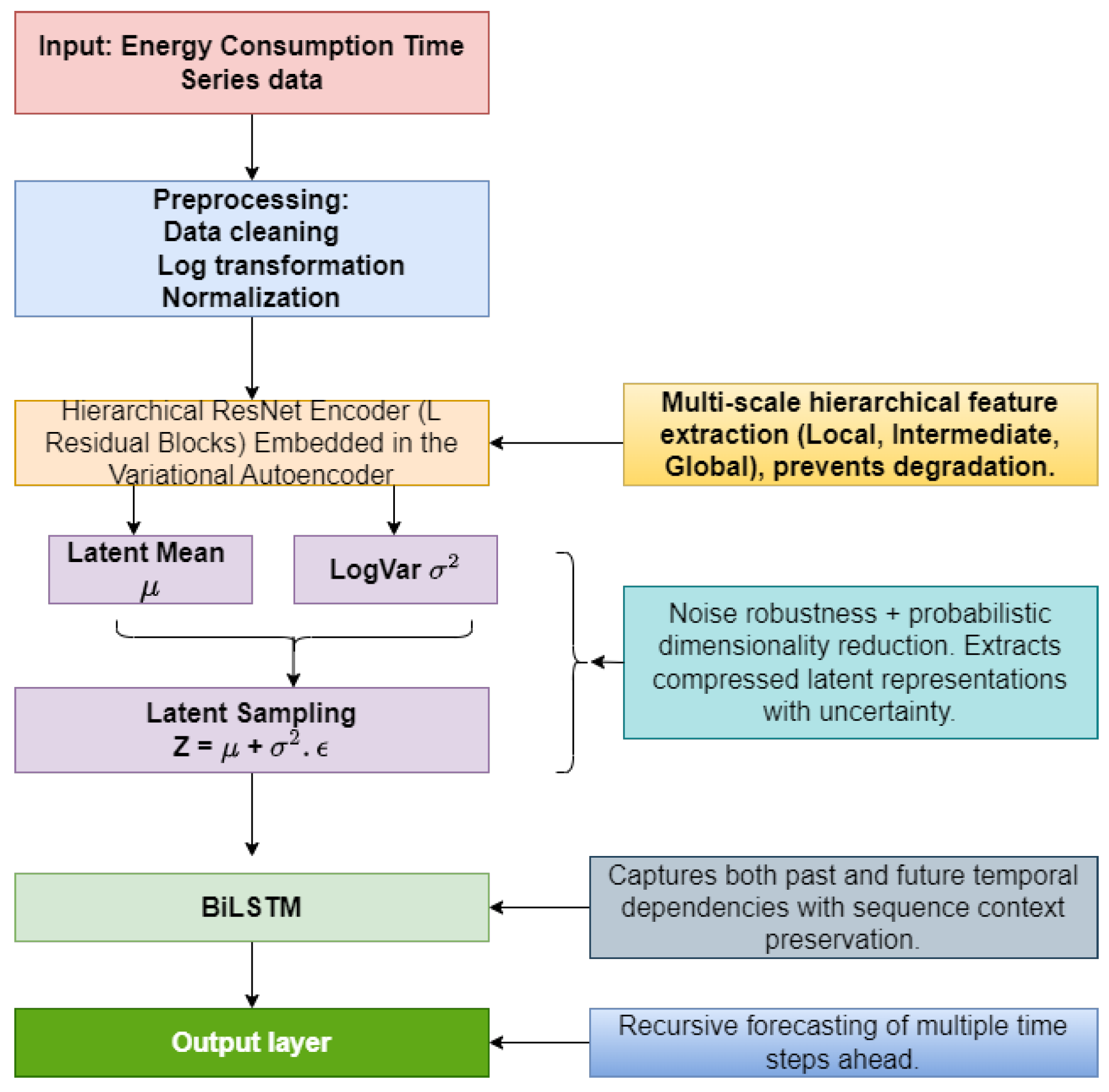
Figure 2.
Illustration of a Residual Neural Network Blocks Architecture.
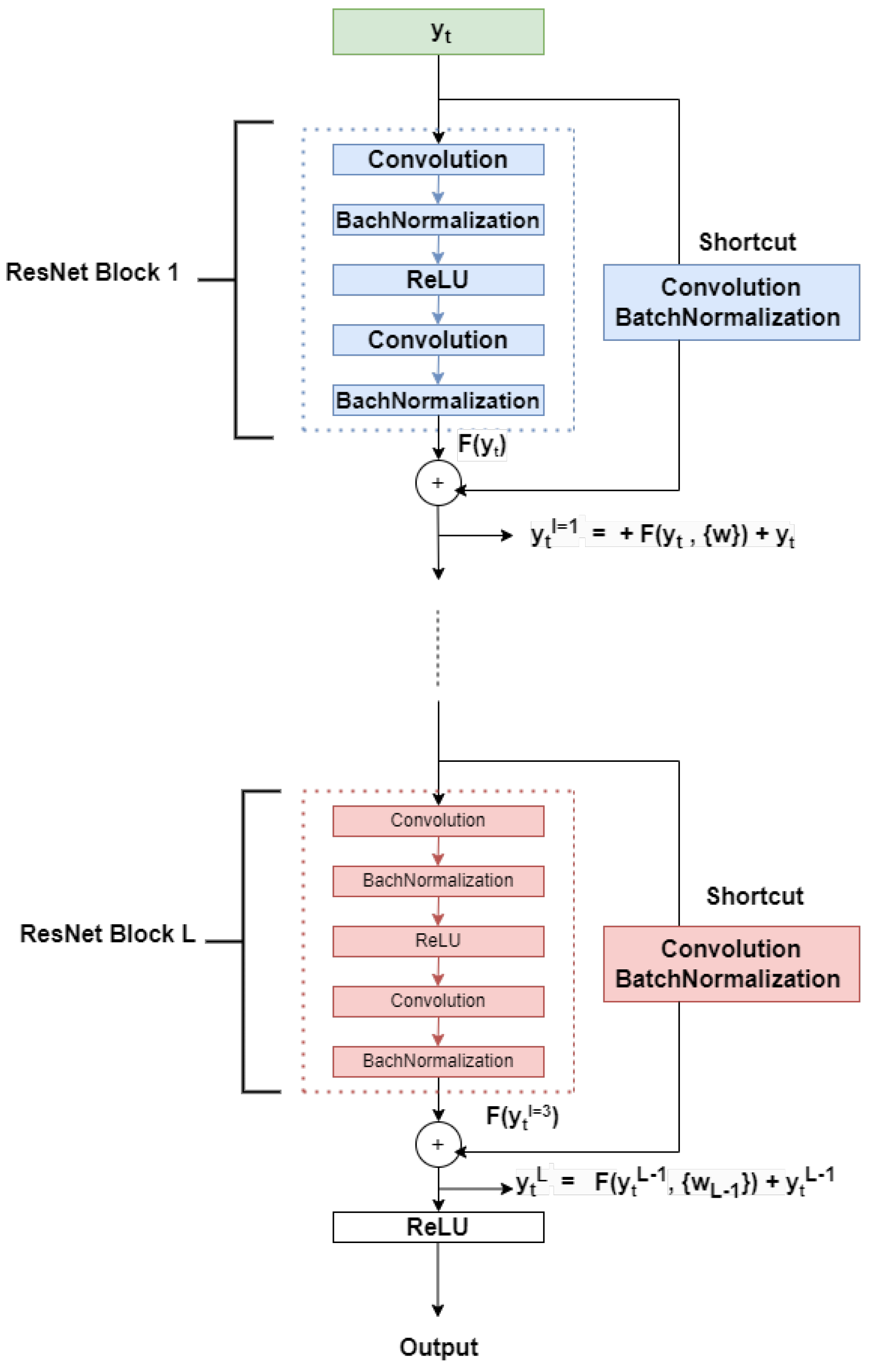
Figure 3.
Variational autoencoder (VAE) network architecture.
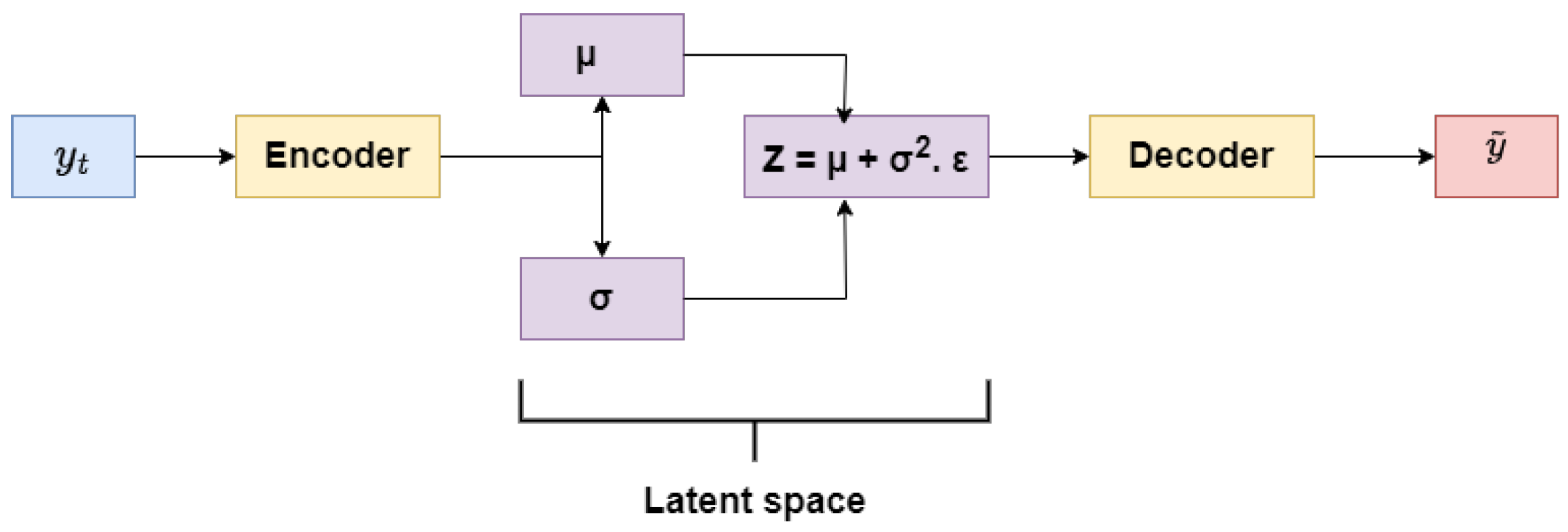
Figure 4.
Recursive algorithm for multi-step ahead forecasting.
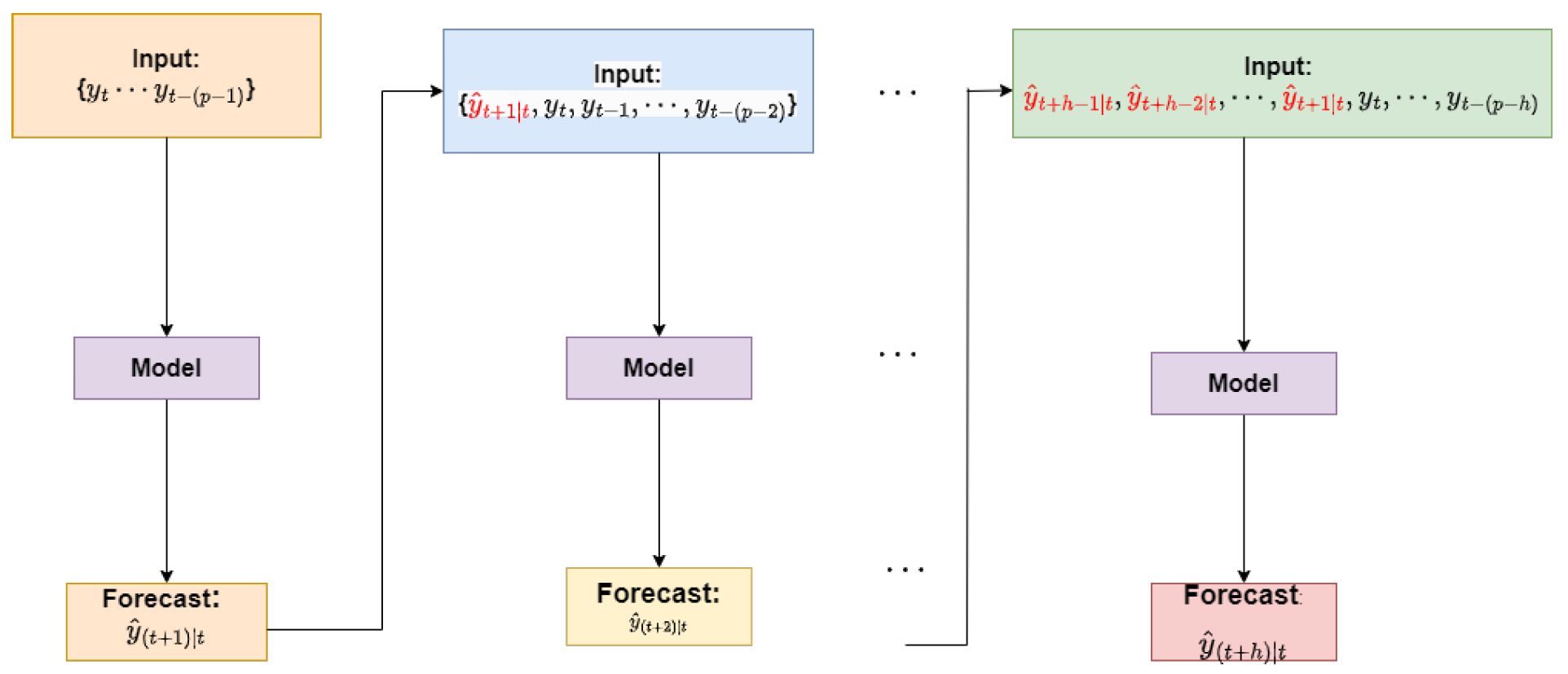
Figure 5.
Complex properties of energy consumption: (a) Hourly energy consumption, (b) Autocorrelation of hourly energy consumption, (c) Daily energy consumption, (d) Autocorrelation of daily energy consumption, (e) Fourier transform of hourly energy consumption, (f) Squared coherence of hourly energy consumption, (g) Fourier transform of daily energy consumption, and (h) Squared coherence of daily energy consumption.
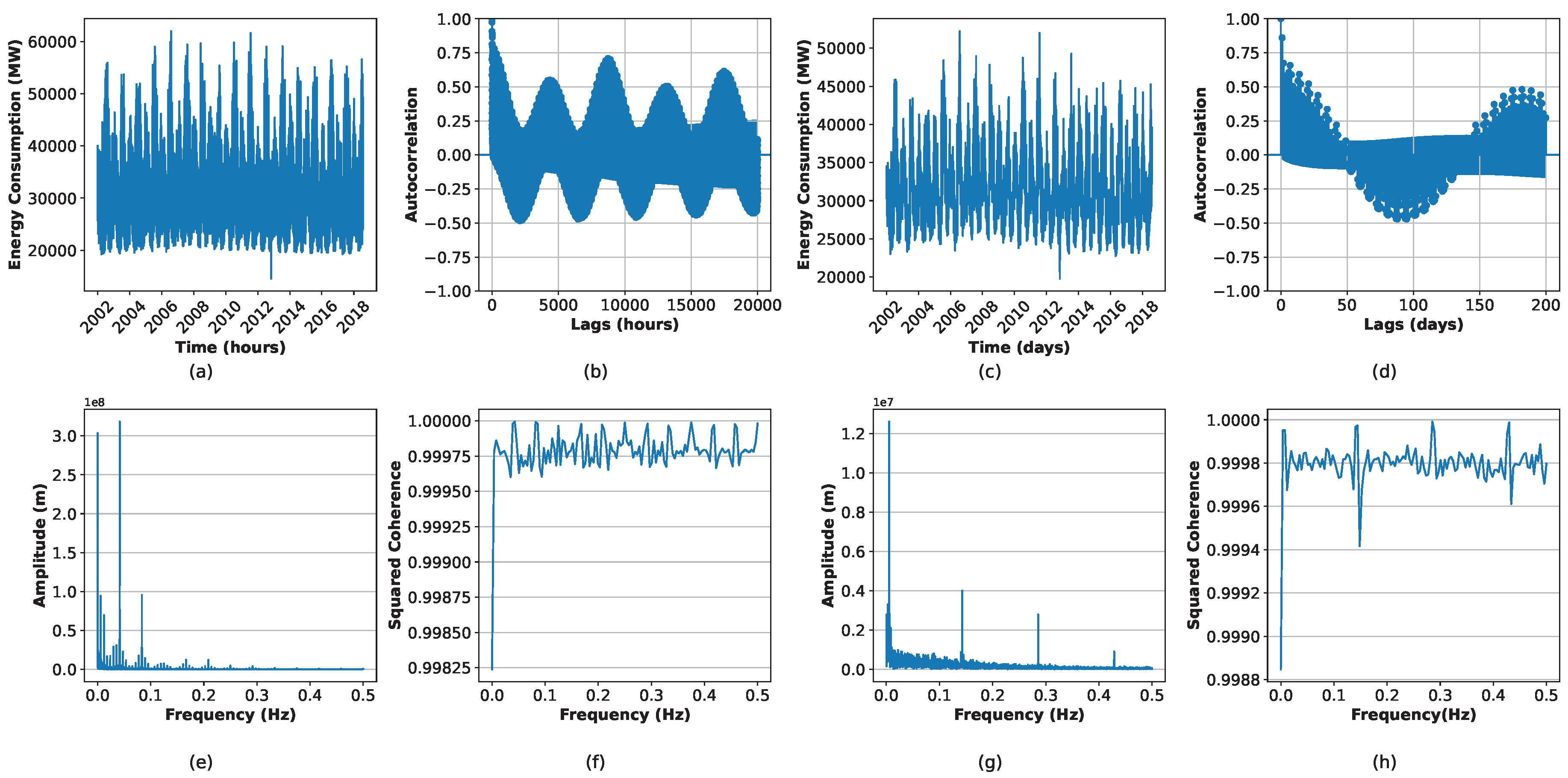
Figure 6.
Visualization of hourly energy consumption forecasting across various models for the next 24 hours.
Figure 6.
Visualization of hourly energy consumption forecasting across various models for the next 24 hours.
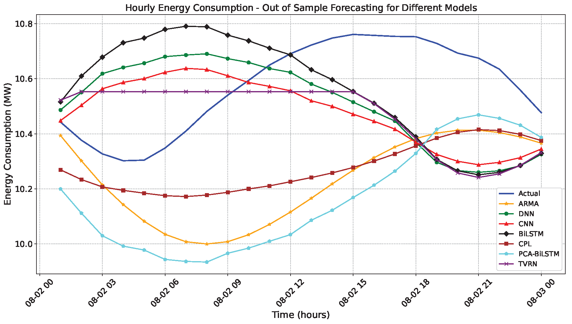
Figure 7.
Visualization of 15-day-ahead daily energy consumption forecasting across various models.
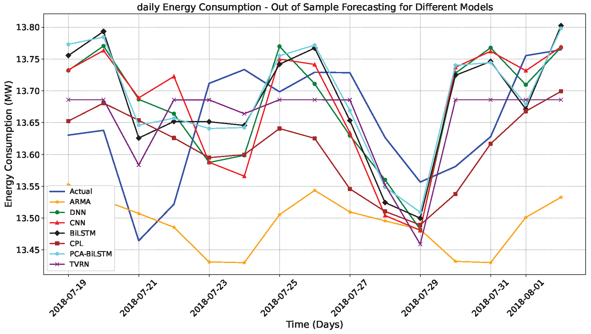

Table 1.
Comparison of Forward and Backward LSTM Gate Operations.
| Operation | Forward LSTM | Backward LSTM |
|---|---|---|
| Forget Gate | ||
| Input Gate | ||
| Output Gate | ||
| Cell Input | ||
| Cell State | ||
| Hidden State |
Note:z represents the latent space vector of VAE at time t, denotes the hidden state at time t, denotes the sigmoid function, and tanh is the hyperbolic tangent function. The weights , , , and and biases , , , are parameters of the model.
Table 2.
Hyperparameters ResNet component used in the hybrid model training.
| Parameter | Value | Description |
|---|---|---|
| Initial Convolution | 64 Filters, Kernel Size 3, Stride 1 | Initial layer settings |
| ResNet Block 1 | 64 Filters, Stride 1, Kernel Size 3 | Includes Shortcut |
| ResNet Block 2 | 32 Filters, Stride 1, Kernel Size 3 | Includes Shortcut |
| ResNet Block 3 | 16 Filters, Stride 1, Kernel Size 3 | Includes Shortcut |
| ResNet Block 4 | 16 Filters, Stride 1, Kernel Size 3 | Includes Shortcut |
| Pooling Type | MaxPooling, Size 2, Stride 1, padding=’same’ | Pooling settings |
| Activation Functions | ReLU, Tanh | Types of activation used |
| Regularization | L2 (0.0001) | Regularization for BiLSTMlayers |
| Batch Normalization | Applied | Used in all ResNet blocks and shortcuts |
Table 3.
The performance of hourly energy forecasting, assessed using RMSE and MAE across different forecasting horizons (h-ahead), with the best results in each row highlighted in bold.
Table 3.
The performance of hourly energy forecasting, assessed using RMSE and MAE across different forecasting horizons (h-ahead), with the best results in each row highlighted in bold.
| Horizon | ARIMA | DNN | BiLSTM | CNN | CPL | PCA-BiLSTM | TVRN |
|---|---|---|---|---|---|---|---|
| RMSE | |||||||
| train | 0.228 | 0.070 | 0.024 | 0.034 | 0.175 | 0.015 | 0.076 |
| h = 1 | 0.052 | 0.079 | 0.028 | 0.032 | 0.259 | 0.021 | 0.003 |
| h = 12 | 0.424 | 0.209 | 0.298 | 0.250 | 0.270 | 0.304 | 0.158 |
| h = 24 | 0.402 | 0.304 | 0.324 | 0.297 | 0.297 | 0.322 | 0.261 |
| MAE | |||||||
| train | 0.182 | 0.058 | 0.023 | 0.027 | 0.139 | 0.013 | 0.038 |
| h = 1 | 0.052 | 0.079 | 0.028 | 0.032 | 0.259 | 0.021 | 0.003 |
| h = 12 | 0.369 | 0.177 | 0.258 | 0.212 | 0.269 | 0.261 | 0.132 |
| h = 24 | 0.363 | 0.269 | 0.291 | 0.264 | 0.296 | 0.288 | 0.224 |
Table 4.
Forecast performance of daily energy data, evaluated using RMSE and MAE across various models and forecasting horizons. Bold indicates the best result in each row.
Table 4.
Forecast performance of daily energy data, evaluated using RMSE and MAE across various models and forecasting horizons. Bold indicates the best result in each row.
| Horizon | ARIMA | DNN | BiLSTM | CNN | CPL | PCA-BiLSTM | TVRN |
|---|---|---|---|---|---|---|---|
| RMSE | |||||||
| train | 0.186 | 0.062 | 0.061 | 0.062 | 0.125 | 0.060 | 0.068 |
| h = 1 | 0.077 | 0.073 | 0.083 | 0.078 | 0.059 | 0.099 | 0.005 |
| h = 7 | 0.180 | 0.128 | 0.114 | 0.125 | 0.200 | 0.118 | 0.079 |
| h = 15 | 0.178 | 0.129 | 0.120 | 0.133 | 0.167 | 0.123 | 0.086 |
| MAE | |||||||
| train | 0.047 | 0.048 | 0.047 | 0.048 | 0.095 | 0.047 | 0.050 |
| h = 1 | 0.077 | 0.073 | 0.083 | 0.078 | 0.059 | 0.099 | 0.005 |
| h = 7 | 0.149 | 0.107 | 0.094 | 0.106 | 0.190 | 0.100 | 0.069 |
| h = 15 | 0.159 | 0.111 | 0.103 | 0.115 | 0.147 | 0.106 | 0.074 |
Disclaimer/Publisher’s Note: The statements, opinions and data contained in all publications are solely those of the individual author(s) and contributor(s) and not of MDPI and/or the editor(s). MDPI and/or the editor(s) disclaim responsibility for any injury to people or property resulting from any ideas, methods, instructions or products referred to in the content. |
© 2025 by the authors. Licensee MDPI, Basel, Switzerland. This article is an open access article distributed under the terms and conditions of the Creative Commons Attribution (CC BY) license (http://creativecommons.org/licenses/by/4.0/).
Copyright: This open access article is published under a Creative Commons CC BY 4.0 license, which permit the free download, distribution, and reuse, provided that the author and preprint are cited in any reuse.


