Submitted:
21 May 2025
Posted:
22 May 2025
You are already at the latest version
Abstract
To address the challenges posed by the volatility and uncertainty of wind power generation, this study presents a hybrid model combining Complete Ensemble Empirical Mode Decomposition with Adaptive Noise (CEEMDAN), Variational Mode Decomposition (VMD), Convolutional Neural Network (CNN), and Bidirectional Long Short-Term Memory (BiLSTM) for wind power forecasting. The model first employs CEEMDAN to decompose the original wind power sequence into multiple scales, obtaining several Intrinsic Mode Functions (IMFs). These IMFs are then classified using sample entropy and k-means clustering, with high-frequency IMFs further decomposed using VMD. Next, the decomposed signals are processed by a CNN to extract local spatiotemporal features, followed by a BiLSTM network that captures bidirectional temporal dependencies. Experimental results demonstrate the superiority of the proposed model over ARIMA, LSTM, CEEMDAN-LSTM, and VMD-CNN-LSTM models. The proposed model achieves a mean squared error (MSE) of 67.145, root mean squared error (RMSE) of 8.192, mean absolute error (MAE) of 6.020, and a coefficient of determination (R2) of 0.9840, indicating significant improvements in forecasting accuracy and reliability. This study offers a new solution for enhancing wind power forecasting precision, which is crucial for efficient grid operation and energy management. Future work will focus on optimizing the model structure and parameters to reduce computational costs and improve robustness, further advancing the application of hybrid models in wind power forecasting.
Keywords:
wind power forecasting
; CEEMDAN
; VMD
; CNN
; BiLSTM
; K-means
1. Introduction
In the global energy structure’s accelerated transition toward low-carbon systems, wind power, with its clean and renewable advantages, has become a key part of power systems [1,2,3]. Statistics from the International Renewable Energy Agency (IRENA) show that China maintained its leading position in global wind power installed capacity as of 2021[4]. However, wind power generation, influenced by complex meteorological conditions and equipment operation status, exhibits significant volatility and uncertainty[5]. This poses severe challenges to grid scheduling, electricity market trading, and equipment maintenance, making high-precision power forecasting technology essential[6].
Currently, wind power forecasting methods are mainly categorized into physical models, statistical models, and data-driven approaches. Physical models, based on aerodynamic principles, have explicit physical meanings but are highly dependent on meteorological and equipment parameters and struggle to capture nonlinear characteristics[7]. Statistical models like ARIMA and SVM predict by fitting historical data but lack adaptability to non-stationary and nonlinear data. In recent years, deep learning has emerged as a new tool for wind power forecasting[8].
Early wind power forecasting studies focused on physical modeling. For instance, a study in [9] built a unit model based on aerodynamics and predicted power using meteorological data. While the physical significance was clear, calibration difficulties in complex terrains and variable weather limited forecasting accuracy. On the statistical modeling front, [10] used ARMA and other time-series methods, relying on data statistical patterns for modeling. This approach was computationally simple but insufficient for non-stationary and nonlinear data. With AI development, machine learning methods gained traction. SVM, through kernel functions, enabled nonlinear fitting. As shown in [11], SVM was applied to wind power forecasting with some success, but its performance heavily relied on parameter tuning and had computational efficiency limits. Deep learning techniques introduced a breakthrough, with LSTM and its variants capturing long-term dependencies in time-series data through gating mechanisms. As demonstrated in [12], LSTM significantly improved forecasting accuracy but had weak spatial feature extraction capabilities. CNN excelled at extracting local spatiotemporal features but fell short in modeling long-term temporal dependencies[13]. To leverage the strengths of different methods, hybrid models became a research hotspot. For example, [14] proposed a VMD-LSTM model that first used variational mode decomposition to extract multi-scale features and then predicted with LSTM, effectively enhancing accuracy. Another study in [15] combined CNN-LSTM to handle spatial and temporal features separately, further refining forecasting outcomes. In China, initial research focused on improving traditional models. For instance, [16] enhanced time-series models’ adaptability to non-stationary data through seasonal adjustments and differencing. In deep learning, [17] introduced attention mechanisms to strengthen LSTM’s focus on key temporal sequences, while [18] improved model robustness through data cleaning.
However, existing methods have limitations. Statistical models like ARIMA are computationally simple but lack adaptability to non-stationary and nonlinear data. Machine learning methods offer strong nonlinear fitting but depend on parameter tuning and have computational efficiency limits. LSTM captures long-term temporal dependencies but weakly extracts spatial features, while CNN effectively extracts local spatiotemporal features but falls short in modeling long-term temporal dependencies. These limitations highlight the need for new solutions in wind power forecasting.
To address these issues, this study proposes a deep forecasting model integrating multi-source information and adaptive decomposition. The model constructs a multi-source data fusion framework, enhances signal decomposition with CEEMDAN and VMD, and designs a CNN-BiLSTM network with dual attention mechanisms to capture key spatiotemporal and equipment status features. Experimental results show that the proposed model achieves superior forecasting accuracy with an MSE of 67.145, RMSE of 8.192, MAE of 6.020, and R² of 0.9840, offering a new technical solution for wind power forecasting.
2. Theoretical Basis
2.1. Ceemdan Algorithm
CEEMDAN (Complete Ensemble Empirical Mode Decomposition with Adaptive Noise) is an adaptive noise complete ensemble empirical mode decomposition method that introduces adaptive noise during the empirical mode decomposition (EMD) process to solve the mode mixing problem of traditional EMD methods when dealing with non-stationary signals [19]. The core of the algorithm is to add white noise to enhance the multi-scale characteristics of the signal, making it easier to separate fluctuations of different frequency components into independent intrinsic mode functions (IMFs). Since the noise cancels out during multiple decompositions, CEEMDAN retains the true characteristics of the signal and is suitable for multi-scale analysis of complex wind power signals with significant fluctuations [20]. The original wind power forecasting data series, affected by meteorological conditions, terrain, and unit characteristics, exhibits strong non-linearity and non-stationarity. CEEMDAN decomposes the original sequence into multiple IMF components, achieving multi-scale separation of complex signals, where high-frequency components reflect short-term rapid fluctuations and low-frequency components reflect long-term trends [19].
The CEEMDAN algorithm steps are shown in Figure 1 and are described as follows:
1)ADDING WHITE NOISE
Add N sets of positive and negative Gaussian white noise vk(t) to the signal y(t), resulting in a new signal y(t)+(-1) qε0vk(t), where q=1,2, ε0 is the noise coefficient, y(t) is the preprocessed original signal, and k=1,2,…,N is the number of times the white noise is added.
2)EMD DECOMPOSITION OF NEW SIGNAL
Perform EMD on the new signal to obtain the first IMF component C1(k) .
3)OVERALL AVERAGE
Compute the overall average of the decomposition results of all new signals to obtain the first IMF component of CEEMDAN.
Calculate Residual: Compute the residual r1(t).
4)REPEAT DECOMPOSITION
Repeat the above steps on the residual r1(t) to obtain subsequent IMF components C2(t), C3(t), ..., until the residual rm(t) becomes a monotonic signal. Ultimately, the original signal y(t) is decomposed into m IMF components and a residual.
SAMPLE ENTROPY CALCULATION
Sample entropy (Sample Entropy) is used to measure the complexity of a time series [21]. The calculation steps are as follows:
1)CONSTRUCTING EMBEDDING VECTORS
Embed the time series x into an m-dimensional space to construct embedding vectors:
where i=1,2,…,N−m+1, and N is the length of the time series.
2)CALCULATING DISTANCES
For each embedding vector Xim, calculate the euclidean distance dij to all other embedding vectors Xim.
3)SETTING SIMILARITY TOLERANCE
Set the similarity tolerance r, typically r=0.2std(x).
4)CALCULATING MATCHING PROBABILITY
For each Xim, calculate the proportion of embedding vectors Cim(r) that satisfy dij ≤ r.
5)DEFINING SAMPLE ENTROPY
The sample entropy is defined as:
2.2. k-Means Clustering
K-means clustering is used to classify IMF components based on sample entropy values, as shown in Figure 2. The calculation steps are as follows:
1) Initialization:Randomly select k samples as the initial cluster centers C1,C2,…,Ck.
2) Sample Assignment: Assign each sample xi to the nearest cluster center
3) Update Cluster Centers: Recalculate the center of each cluster
where nj is the number of samples in cluster j.
4) Iteration: Repeat the sample assignment and cluster center update steps until the cluster centers no longer change or the maximum number of iterations is reached.
2.3. VMD Algorithm
VMD (Variational Mode Decomposition) is a method that transforms the signal decomposition problem into solving the center frequency and bandwidth of each mode by constructing a variational optimization model, thus avoiding endpoint effects and mode mixing. It is suitable for multi-scale analysis of nonlinear and non-stationary signals [22,23]. For the secondary decomposition of high-frequency IMF components obtained from CEEMDAN, a frequency-domain bandwidth constraint is introduced to separate high-frequency components, generating sub-modes with explicit frequency characteristics and stable trends. This helps the model to better capture the dynamic changes in wind power. The combination of VMD with CEEMDAN forms a “coarse-to-fine” signal processing framework. The algorithm steps are shown in Figure 3 and are described as follows:
1) Assume the signal f(t) to be processed:
In the formula, ωk is the center frequency of the k-th mode, and δ(t) is the unit impulse function. Here, k is the number of modes obtained from the decomposition, and the input signal f(t) is decomposed into discrete sub-signals (modes) μk.
2) Solve the variational problem:
where α is the penalty factor, λ(t) is the Lagrange multiplier, and the last term is an additional constraint. The parameters are initialized and updated according to equations (12)-(14) until equation (15) is satisfied.
where τ is the noise tolerance and ε is the convergence criterion.
2.4. Spectral Analysis
Spectral analysis is used to display the frequency characteristics of each decomposed modal component. The mathematical expressions are as follows:
1) Fast Fourier Transform (FFT): Perform FFT on each modal component uk(t):
2) Amplitude Spectrum: Calculate the amplitude of the FFT result:
3) Set the frequency range to [0, fs/2], where fs is the sampling frequency.
2.5. CNN Algorithm
The convolutional neural network (CNN) consists of an input layer, convolutional layers, a ReLU activation layer, max-pooling layers, a flattening layer, a BiLSTM layer, a dropout layer, fully connected layers, and a regression layer. This structure enables the CNN to effectively capture the spatiotemporal correlation characteristics in wind power forecasting [24,25]. The CNN learns the nonlinear relationships between wind direction, wind speed, and power, identifying power response patterns associated with specific wind direction combinations. The spatial features extracted by the CNN serve as inputs to the BiLSTM, allowing it to integrate historical and future information through its gating mechanism. This combination enhances the accuracy of predicting the dynamic changes in wind power.
2.6. BiLSTM Algorithm
The bidirectional long short-term memory (BiLSTM) network enhances time series forecasting by processing data in both forward and backward directions, creating a bidirectional information flow. This allows the model to learn from both past and future data simultaneously [26,27]. The forward network processes the input sequence in chronological order, capturing feature evolutions from past to present, while the backward network processes the data in reverse, uncovering hidden relationships from future to past. In wind power forecasting, BiLSTM’s bidirectional processing enables it to capture both historical power fluctuations and potential future meteorological impacts. The forward network learns the temporal patterns of historical power and meteorological data, while the backward network infers current key features from future data, improving forecasting accuracy.
Among them, and represent the forward and backward LSTM outputs, respectively. wt and vt are the output weights of each hidden layer, and LSTM(•) denotes the LSTM calculation process. The network structure of BiLSTM is shown in Figure 4. w1 to w3 and v1 to v3 are the hidden layer weights of the forward and backward LSTMs, x1 to x3 are the network input values, and y1 to y3 are the network output values.
3. Construction CEEMDAN- VMD -CNN- BILSTM Model
3.1. Model Framework Design
The core architecture of the CEEMDAN-VMD-CNN-BiLSTM model is shown in Figure 5.
1) SIGNAL DECOMPOSITION
Initially, the CEEMDAN algorithm is employed to perform multi-scale decomposition on the original wind power sequence, generating Intrinsic Mode Function (IMF) components at different frequencies.Sample Entropy is used to measure the complexity of each IMF component, followed by k-means clustering to group similar IMFs. Based on Sample Entropy values, the IMFs are classified into high-frequency, medium-frequency, and low-frequency groups. High-frequency IMFs are then further decomposed using VMD for secondary decomposition.
2) CNN SPATIO-TEMPORAL FEATURE EXTRACTION
Convolutional layers are applied to the VMD-secondary decomposed sequences to extract local spatio-temporal features (e.g., wind speed mutations, wind direction patterns). Pooling layers compress feature dimensions and enhance robustness. After convolution, data is passed through a ReLU activation layer, followed by max-pooling. The pooled feature maps are then flattened into one-dimensional vectors for input into subsequent fully connected layers.
3) BiLSTM SEQUENCE MODELING
The flattened data enters the BiLSTM layer, which processes both forward and backward temporal information simultaneously. The hidden state of the last time step is output as a feature representation of the entire sequence.The BiLSTM output is passed through a Dropout layer to prevent overfitting and improve generalization.
4) FORECASTING OUTPUT
The Dropout layer output is fed into a fully connected layer, which calculates and outputs predicted values based on input features. Finally, the regression layer receives the fully connected layer output and generates the final forecasting results, completing the mapping from input data to forecasting.
3.2. Data Processing and Preparation
Generally, the original wind power forecasting data sequence contains noise, outliers, and missing values, and the dimensions and scales of different variables may also vary. Therefore, data cleaning and preprocessing are necessary [28]. For data points that deviate significantly from the normal range, thresholds are set for judgment and elimination. For example, in wind speed data, wind speeds exceeding many times the rated wind speed of the fan or negative wind speeds should be regarded as invalid data. The 3σ criterion is used to check and process data points whose deviation from the mean exceeds three times the standard deviation. Normalization ensures that data is within the same order of magnitude, facilitating subsequent model training and analysis. This study employs the min-max normalization method, with the formula:
where x represents the original wind power forecasting data sequence, xmin and xmax are the minimum and maximum values of the variable in the dataset, respectively, and xnorm is the normalized data. Through this approach, data for variables such as wind speed, wind direction, temperature, and wind power are normalized to the interval [0, 1], making the data of different variables comparable and contributing to improving the training effect and forecasting accuracy of the model.
In this study, 75% of all data is used as the training set, and 25% is used as the test set.
3.3. Model Parameter Setting and Optimization
1)CEEMDAN ALGORITHM PARAMETER SELECTION
For the CEEMDAN algorithm, the key parameters include the white noise intensity and ensemble averaging times. The selection of white noise intensity directly affects the feature enhancement effect at different scales and the mitigation of modal aliasing. If the white noise intensity is too low, it may fail to effectively enhance signal features, leaving modal aliasing unresolved. Conversely, excessive intensity may introduce noise interference and degrade decomposition accuracy [29]. Through multiple experimental comparisons, the white noise intensity is set to 0.15, and the ensemble averaging times are set to 500 in this study.
2)VMD ALGORITHM PARAMETER SELECTION
The main parameters of the VMD algorithm are the number of modes k and the penalty factor ɑ. The selection of k depends on the signal complexity and frequency components. An excessively small k may insufficiently decompose the signal, while an excessively large k may over-decompose it [30]. For high-frequency IMFs decomposed by CEEMDAN, spectral analysis preliminarily determines k within the range of 3–6. The penalty factor ɑ balances signal reconstruction error and modal bandwidth. A larger ɑ penalizes reconstruction errors more strictly, resulting in narrower modal bandwidths and higher precision but increased computational cost. A smaller ɑ reduces bandwidth constraints and computational load but may compromise decomposition accuracy [31]. Through experimental debugging, k = 4 and ɑ=2000 are adopted in this study.
3) CNN ALGORITHM PARAMETER SELECTION
CNN parameters include convolution kernel size, stride, number of convolutional layers, max-pooling layer size, and pooling stride [32]. A 3×3 convolution kernel is used with a stride of 1 to retain detailed sequence features. The ReLU activation function introduces nonlinearity to enable complex pattern learning. A 2×2 max-pooling layer with a stride of 2 preserves prominent features. The Dropout layer randomly discards 10% of inputs to prevent overfitting. The fully connected layer outputs a single unit for regression tasks, generating forecasting values.
4) BiLSTM ALGORITHM PARAMETER SELECTION
BiLSTM parameters mainly include the number of hidden layer nodes, learning rate, and regularization parameter. The number of hidden layer nodes determines the model’s ability to learn temporal features. Insufficient nodes limit representational capacity, while excessive nodes increase complexity and overfitting risk [33]. In this study, the number of hidden layer nodes is set to 128 based on data length and complexity. The learning rate is determined as 0.001 through experiments, and the regularization parameter is set to 0.00001.
4. Experimental Results and Analysis
4.1. Model Performance Evaluation Metrics
To assess the CEEMDAN-VMD-CNN-BiLSTM model’s performance, we use MSE, RMSE, MAE, and R². These metrics are calculated as follows:
MSE (Mean Squared Error),
RMSE (Root Mean Squared Error) :
MAE (Mean Absolute Error) :
R² (Coefficient of Determination) :
where n is the number of samples, yi is the true value, is the predicted value, and is the mean of the true values.
These metrics help evaluate the model’s reliability and accuracy in wind power forecasting.
4.2. Signal Decomposition Experiment
To validate the effectiveness of the CEEMDAN-VMD-CNN-BiLSTM model in wind power forecasting, this paper takes a wind farm as an example. Data including wind speeds (m/s) at heights of 10m, 30m, 50m, 70m and hub height, wind directions at the same heights, temperature, air pressure, humidity, and power generation were collected from March 1st to April 30th, 2021. The data sampling interval was 15 minutes. After pre-processing, a total of 5,760 sets of data were obtained, with 4,320 sets in the training set and 1,440 sets in the test set.
As demonstrated in Figure 6, the CEEMDAN decomposition approach decomposed the wind power series into 12 IMFs, reflecting its effectiveness in multi-scale feature extraction. These components captured the fluctuation characteristics of wind power at different frequency scales.
Then, the sample entropy was used to calculate the complexity of each IMF component. Through k-means clustering, the IMF components were divided into three groups: high-frequency, medium-frequency, and low-frequency, to handle signal features in different frequency ranges, as shown in Figure 7. For the high-frequency IMF components, VMD decomposition was further applied to more precisely extract the high-frequency detailed information in the signal. The VMD decomposition results are shown in Figure 8. The frequency characteristics of each sub-mode are more distinct, and the trends are more stable, which helps the model to more acutely capture the dynamic change patterns of wind power. The spectrum analysis results are shown in Figure 9. The amplitude spectra of each modal component were calculated through the Fast Fourier Transform (FFT), visually presenting the frequency distribution of each modal component and verifying the effectiveness of VMD decomposition.
The results show that the CEEMDAN-VMD secondary decomposition has significant advantages in signal decomposition and feature extraction. Through multi-scale decomposition and feature extraction, this model effectively reduces the complexity and volatility of the original data, providing high-quality input features for subsequent forecasting tasks.
4.3. Comparison with Other Models
To conduct a comprehensive assessment of the CEEMDAN-VMD-CNN-BiLSTM model’s performance, it was pitted against several common wind power forecasting models. These included the traditional ARIMA model, the single LSTM model, and combined models such as CEEMDAN-LSTM and VMD-CNN-LSTM. Under identical experimental conditions, each model was employed to make forecasting using the test-set data, and forecasting error metrics were computed. Visual analysis was carried out through figures 10, 11, and 12.
Figure 10 presents the forecasting performance of each model on the training set. It is evident from the figure that the forecasting curve of the model proposed in this paper is the closest to the true-value curve, indicating that it demonstrates a high-level fitting capability during the training phase.
Figure 11 further validates the generalization ability of the proposed model on unseen test data. The forecasting curve not only aligns with the overall trend of the true values but also performs remarkably well in predicting short-term fluctuations and peaks. This confirms the model’s outstanding ability to capture the dynamic changes in wind power.
Figure 12 offers a straightforward display of the forecasting errors of the proposed model. The error distribution of the model is concentrated, and the error values are the smallest, suggesting that its forecasting results are highly stable and accurate.
4.4. Results Discussion
The CEEMDAN-VMD-CNN-BiLSTM model excels in wind power forecasting due to its effective decomposition and feature extraction. However, it has limitations such as high computational complexity and data dependency. Future work will focus on optimizing the model to reduce computational costs and enhance robustness.
5. Conclusions
The CEEMDAN-VMD-CNN-BiLSTM model proposed in this study combines multi-scale decomposition with deep learning, significantly enhancing the accuracy of wind power forecasting. Initially, the model uses CEEMDAN to roughly decompose the original sequence, generating multi-scale IMF components. Then, based on sample entropy calculation and K-means clustering, the IMFs are classified to effectively distinguish high-frequency, medium-frequency, and low-frequency components. For high-frequency IMFs, VMD is further introduced for fine decomposition to extract more representative detailed features. After CNN extracts local spatio-temporal features, BiLSTM captures bidirectional temporal dependencies, ultimately achieving high-precision forecasting. Experimental results show that this model outperforms comparative models in terms of indicators such as MSE (67.145), RMSE (8.192), MAE (6.020), and R² (0.9840), verifying the effectiveness of the integration of multi-scale decomposition and deep networks. This study provides a new technical path for wind power forecasting.
Although the model proposed in this paper has a good effect in the field of wind power forecasting, multiple ensemble averages of CEEMDAN, variational iterative solutions of VMD, and matrix operations during the training of overlapping CNN and BiLSTM all consume a large amount of computational resources. In addition, the model also has a data dependence problem. In the future, a fast ensemble strategy based on empirical mode decomposition can be developed to reduce the number of CEEMDAN ensembles and continue to improve the forecasting ability of the model.
Author Contributions
Conceptualization, Guoping Chen; Formal analysis, Jiwu Wang; Methodology, Guoping Chen; Project administration, Guoping Chen; Resources, Zhanhu Ning and Yuan Luo; Software, Zhanhu Ning; Supervision, Zhanhu Ning; Writing – review & editing, Guoping Chen. All authors will be updated at each stage of manuscript processing, including submission, revision, and revision reminder, via emails from our system or the assigned Assistant Editor.
Data Availability Statement
Data are contained within the article.
Conflicts of Interest
The authors declare no conflicts of interest. The funders had no role in the design of the study; in the collection, analyses, or interpretation of the data; in the writing of the manuscript; or in the decision to publish the results.
References
- X. Zhou, S. Chen, Z. Lu, et al., Technical characteristics of China’s new generation power system in energy transition. Proc. CSEE, 2018, 38, 1893–1904.
- Z. Jizhong, H. Dong, S. Li, et al., Review of data-driven load forecasting for integrated energy system. Proc. CSEE, 2021, 41, 7905–7923.
- M. Yang, D. Wang, X. Wang, et al., Ultra-short-term wind power prediction model based on hybrid data-physics-driven approach. High Volt. Eng., 2024, 50, 5132–5141.
- Y. Zou, Survey of wind power output forecasting technology. IEEE Trans. Sustain. Energy, 2021, 13, 890–901.
- J. Li, X. Hu, J. Qin, et al., Ultra-short-term wind power prediction based on multi-head attention mechanism and convolutional model. Power Syst. Prot. Control, 2023, 51, 56–62.
- D. Wang, Z. Lu, Q. Jia, Medium-long-term wind power prediction based on multi-model optimized combination. Renew. Energy, 2018, 36, 678–685.
- R. Mei, Z. Lyu, W. Gu, et al., Short-term wind power prediction based on principal component analysis and spectral clustering. Autom. Electr. Power Syst., 2022, 46, 98–105.
- H. Chen, H. Li, T. Kan, et al., Ultra-short-term wind power prediction considering temporal characteristics using deep wavelet-temporal convolutional network. Power Syst. Technol., 2023, 47, 1653–1665.
- X. Shen, C. Zhou, X. Fu, Wind speed prediction of wind turbine based on the internet of machines and spatial correlation weight. Trans. China Electrotech. Soc., 2021, 36, 1782–1790, 1817.
- S. Liu, Y. Zhu, K. Zhang, et al., Short-term wind power prediction based on error-corrected ARMA-GARCH model. Acta Energiae Solaris Sin., 2020, 41, 268–275.
- R. Huang, Z. Yu, Y. Deng, et al., Short-term wind speed prediction based on SVM under different feature vectors. Acta Energiae Solaris Sin., 2014, 35, 866–871.
- W. Wang, H. Liu, Y. Chen, et al., Wind power prediction based on LSTM recurrent neural network. Renew. Energy, 2020, 38, 1187–1191.
- C. Liang, Y. Liu, J. Zhou, et al., Multi-point wind speed prediction method within wind farm based on convolutional recurrent neural network. Power Syst. Technol., 2021, 45, 534–542.
- D. Wang, X. Fu, S. Du, Ultra-short-term wind power prediction based on adaptive VMD-LSTM. J. Nanjing Univ. Inf. Sci. Technol., 2025, 17, 74–87.
- X. Liao, C. Chen, J. Wu, Spatiotemporal combined prediction model for wind farms based on CNN-LSTM and deep learning. Inf. Control, 2022, 51, 498–512. [CrossRef]
- L. Li, G. Gao, W. Wu, et al., Short-term day-ahead wind power prediction method considering feature reorganization and improved Transformer. Power Syst. Technol., 2024, 48, 1466–1480.
- X. Liao, J. Wu, C. Chen, Short-term wind power prediction model combining attention mechanism and LSTM. Comput. Eng., 2022, 48, 286–297, 304.
- S. Wang, H. Liu, G. Yu, Short-term wind power combination forecasting method based on wind speed correction of numerical weather prediction. Front. Energy Res., 2024, 12, 1391692.
- P. Flandrin, E. Torres, M. A. Colominas, A complete ensemble empirical model decomposition with adaptive noise, in:2011 IEEE Int. Conf. Acoust. Speech Signal Process., IEEE, Prague, 2011:pp.4144–4147.
- Y. Liu and X. Chen, Short-term wind speed and power forecasting using empirical mode decomposition and least squares support vector machine. Renewable Energy, 2012, 50, 1–7. [Google Scholar]
- Y. Li, J. Li, and Y. Wang, Fault diagnosis of rolling bearings using sample entropy and convolutional neural networks. Mechanical Systems and Signal Processing, 2020, 135, 106418. [Google Scholar]
- A. Alkesaiberi, F. Harrou, and Y. Sun, Efficient wind power prediction using machine learning methods: A comparative study. Energies, 2021, 15, 1–23. [Google Scholar]
- X. Xu, T. Pan, and D. Wu, Wind speed noise reduction in wind farm based on variational mode decomposition. Energy, 2018, 179, 263–274. [Google Scholar]
- X. Li, K. Li, S. Shen, and Y. Tian, Exploring time series models for wind speed forecasting: A comparative analysis. Wind Energy Science, 2023, 8, 1071–1131. [Google Scholar]
- A. Zhu, X. Li, Z. Mo, and R. Wu, Wind power prediction based on a convolutional neural network. Journal of Renewable Energy, 2016, 108, 482–490. [Google Scholar]
- Z. Hameed and B. Garcia-Zapirain, Sentiment classification using a single-layered BiLSTM model. IEEE Access, 2020, 8, 73992–74001. [Google Scholar] [CrossRef]
- N. E. Michael et al., A cohesive structure of bidirectional long-short-term memory (BiLSTM)-GRU for predicting hourly solar radiation. Renewable Energy, Article ID 119943, 2024.
- J. P. Amezquita-Sanchez, Short-term wind power prediction based on anomalous data cleaning and optimized LSTM network. Journal of Renewable Energy, 2023, 210, 45–53. [Google Scholar]
- B. Wenjun and C. Yingjie, Denoising of blasting vibration signals based on CEEMDAN-ICA algorithm. Scientific Reports, 2023, 13, 20928. [Google Scholar] [CrossRef]
- K. Dragomiretskiy and D. Zosso, Variational mode decomposition. IEEE Transactions on Signal Processing, 2013, 62, 531–537. [Google Scholar]
- A. Yinet et al., Adaptive parameter selection for VMD based on central frequency aggregation. Journal of Engineering and Applied Science (RESE), 2023, 12, 45–56. [Google Scholar]
- M. Dong, & J. Han. HAR-Net: Fusing Deep Representation and Hand-crafted Features for Human Activity Recognition. arXiv:1810.11526, 2018.
- Z. Huang, C Gu,.J. Peng, Y. Wu. A Statistical Prediction Model for Sluice Seepage Based on MHHO-BiLSTM. Water, 2024, 16, 191. [Google Scholar] [CrossRef]
Figure 1.
Flow chart for CEEMDAN algorithm.
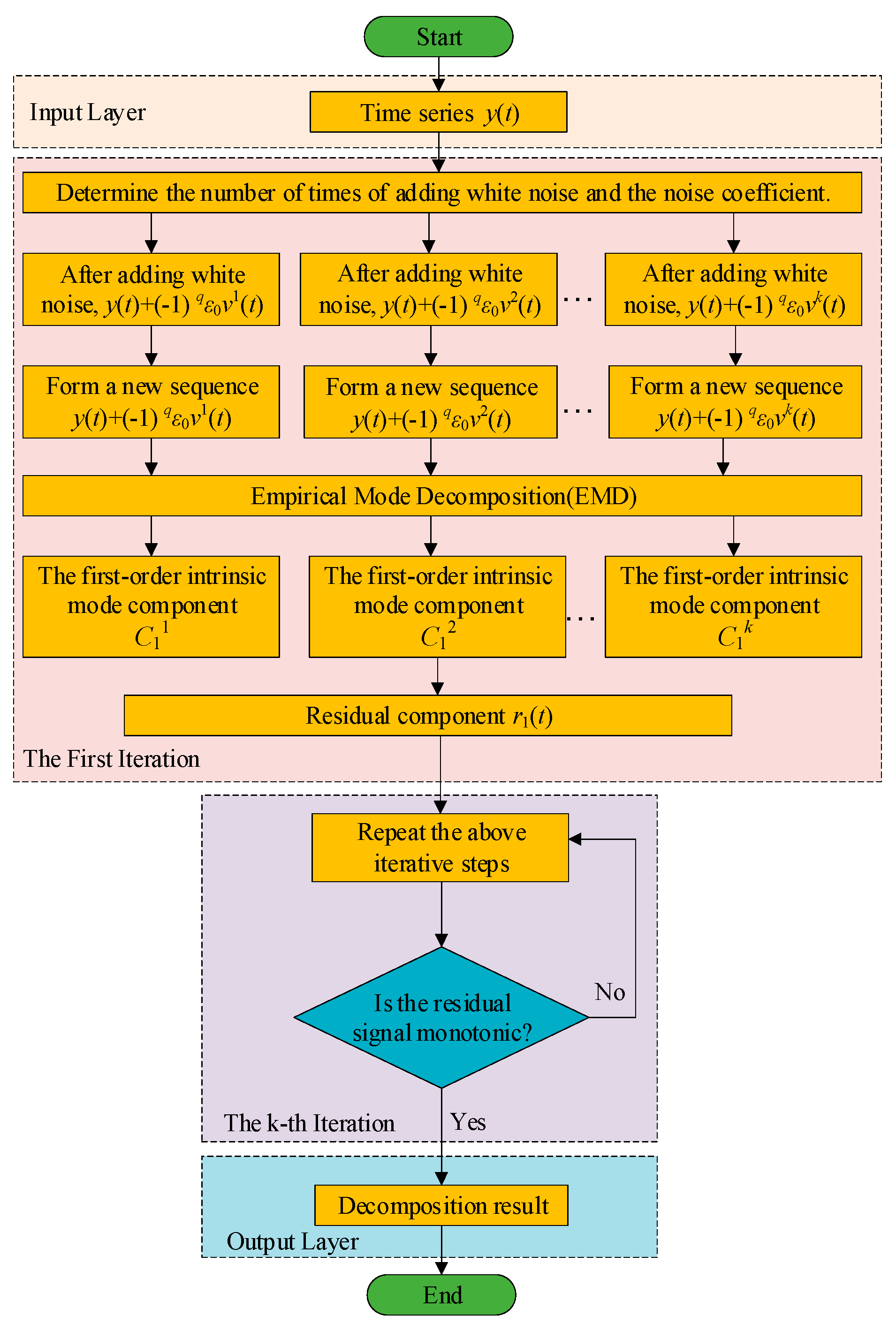
Figure 2.
Flow chart of k-means clustering algorithm.
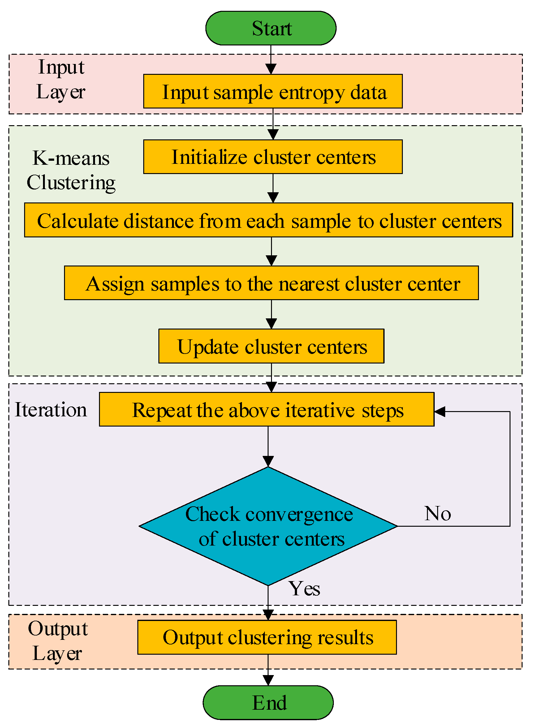
Figure 3.
VMD algorithm flow chart.
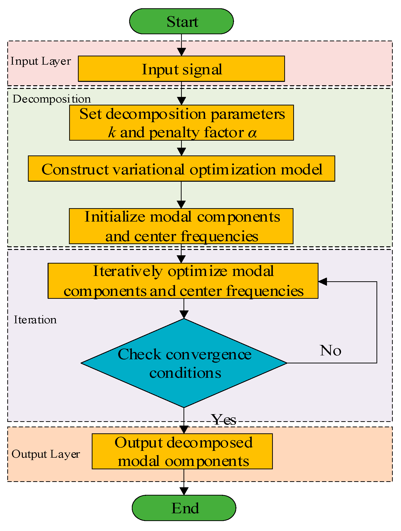
Figure 4.
BiLSTM structure.
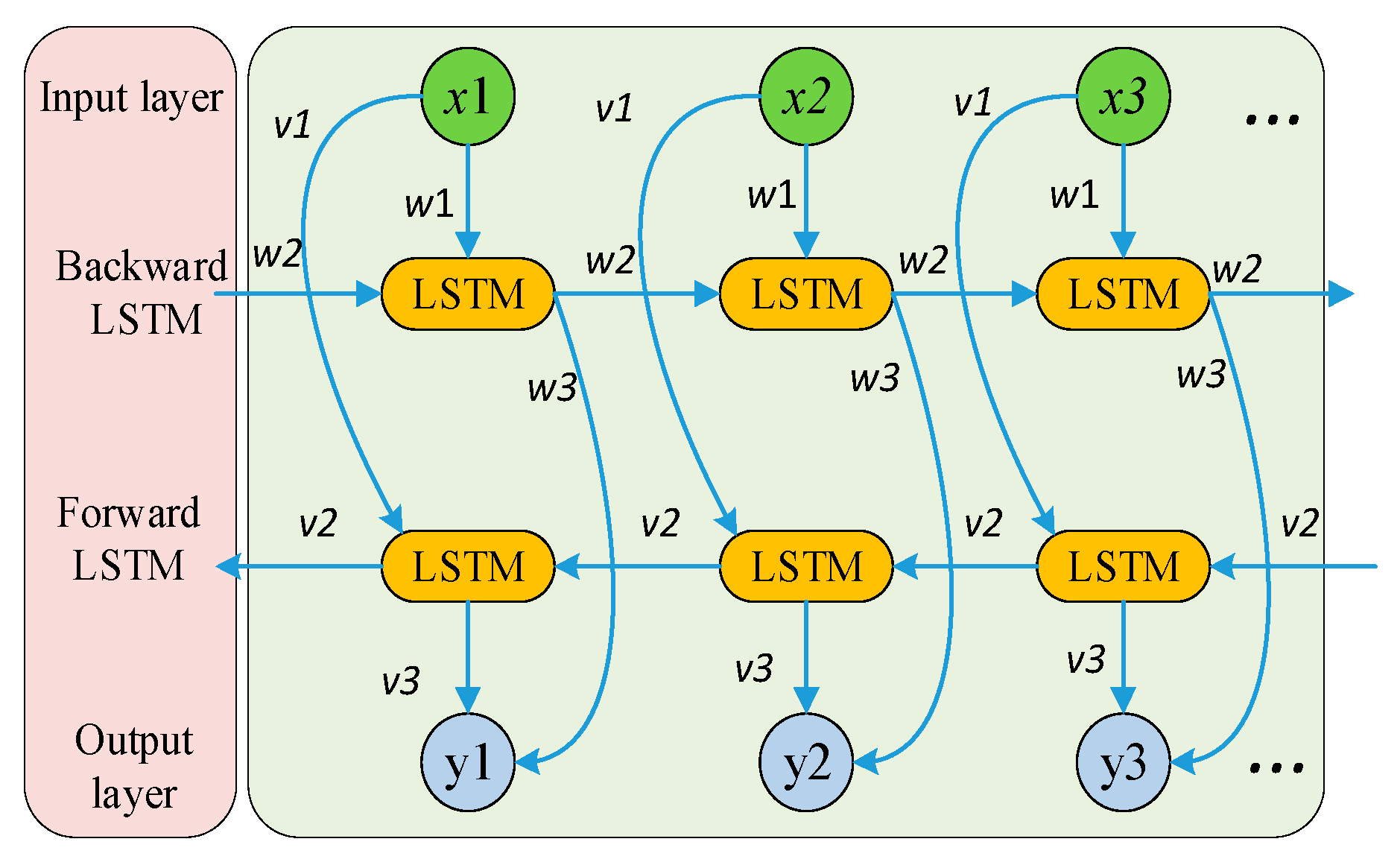
Figure 5.
CEEMDAN-VMD-CNN-BiLSTM Model structure.
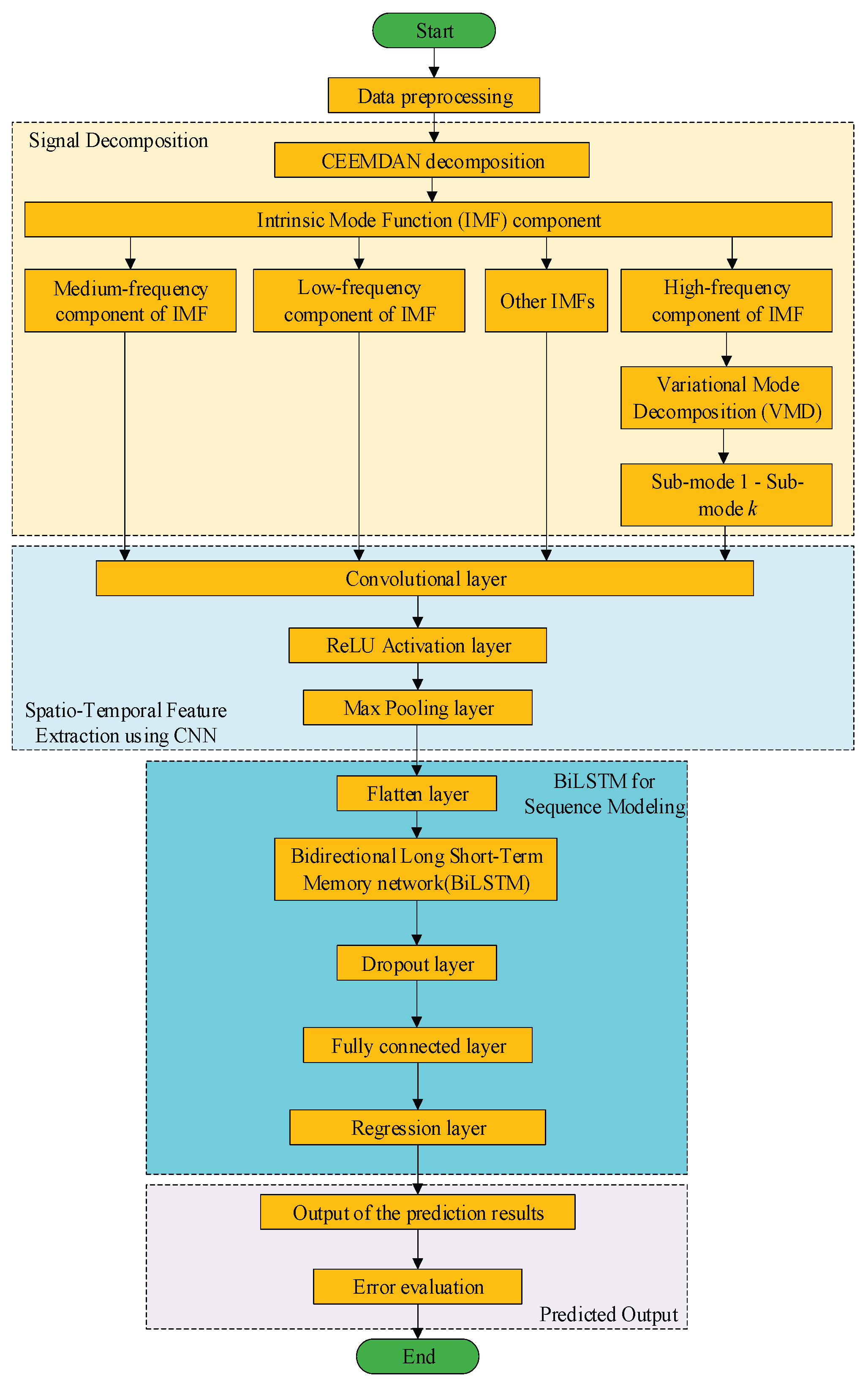
Figure 6.
CEEMDAN decomposition of wind power data.
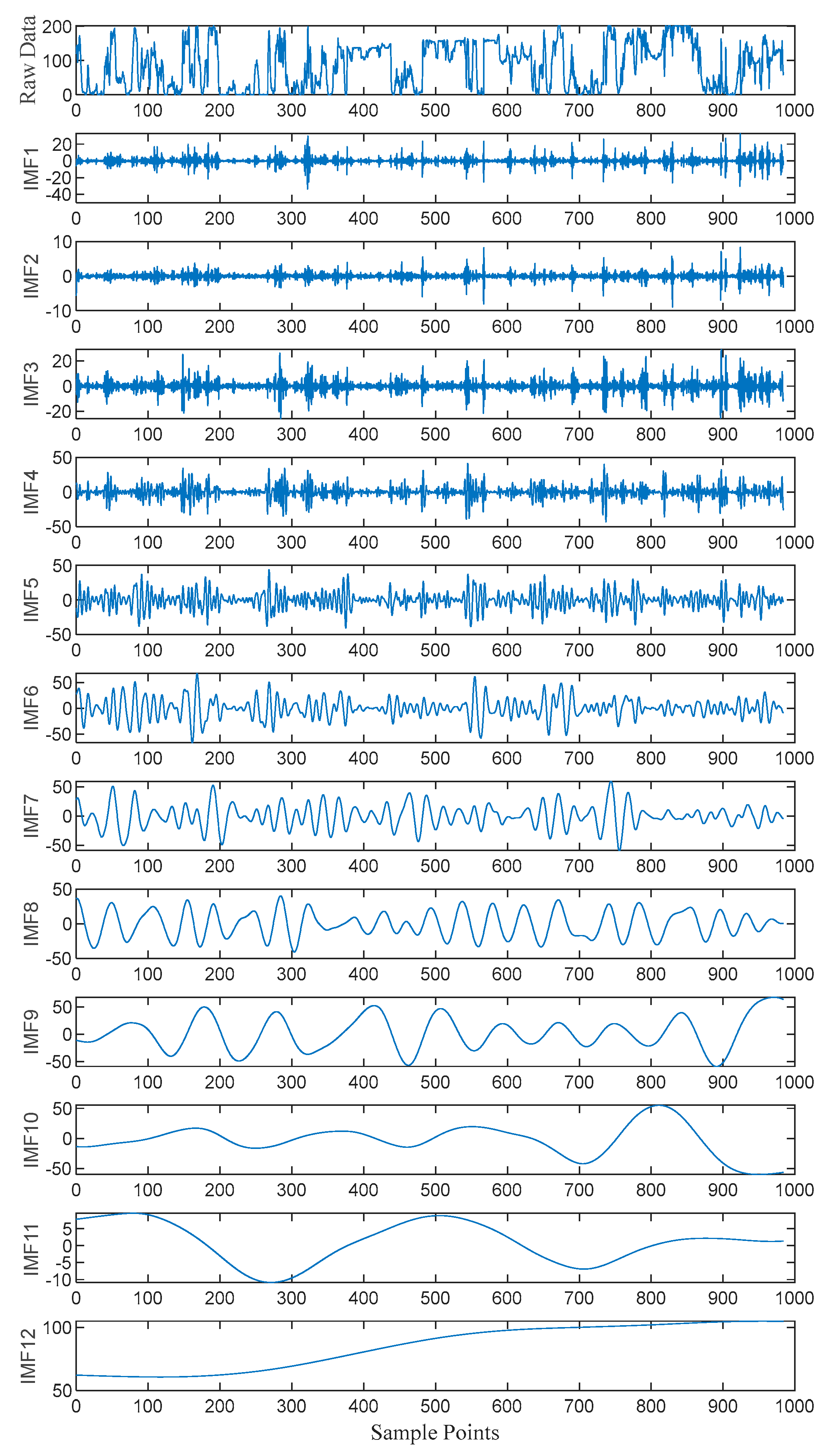
Figure 7.
K-means clustering of IMF components.
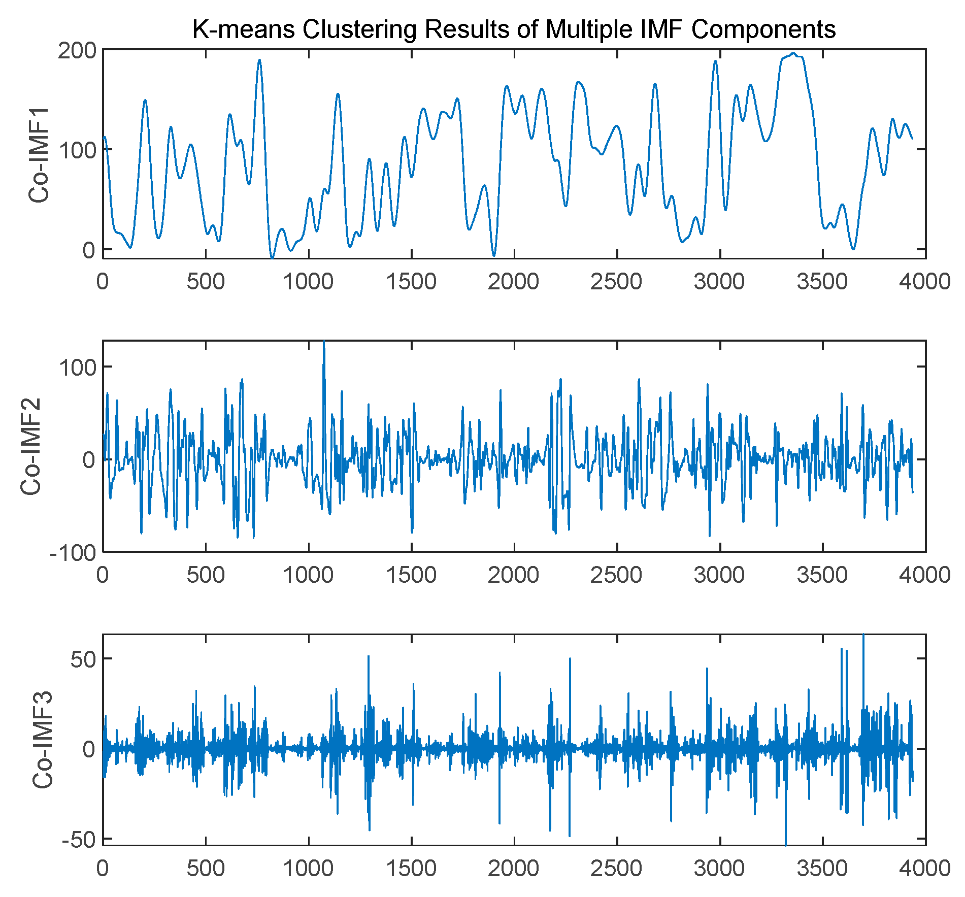
Figure 8.
VMD secondary decomposition.
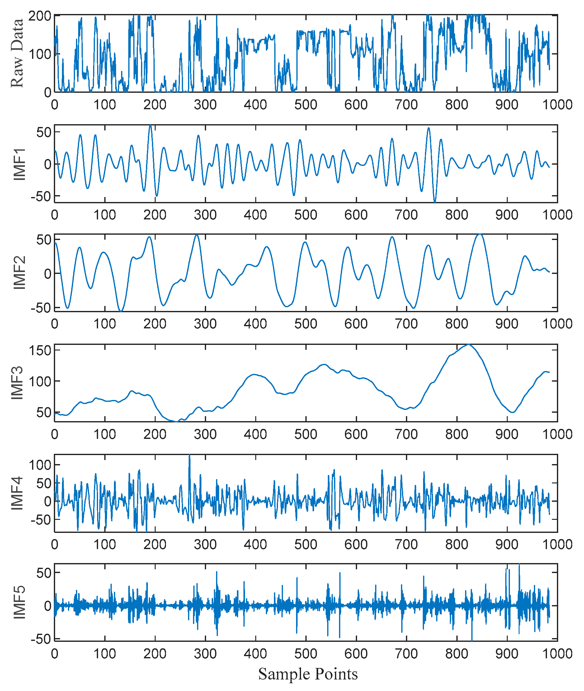
Figure 9.
VMD Secondary Decomposition IMF Spectrum.
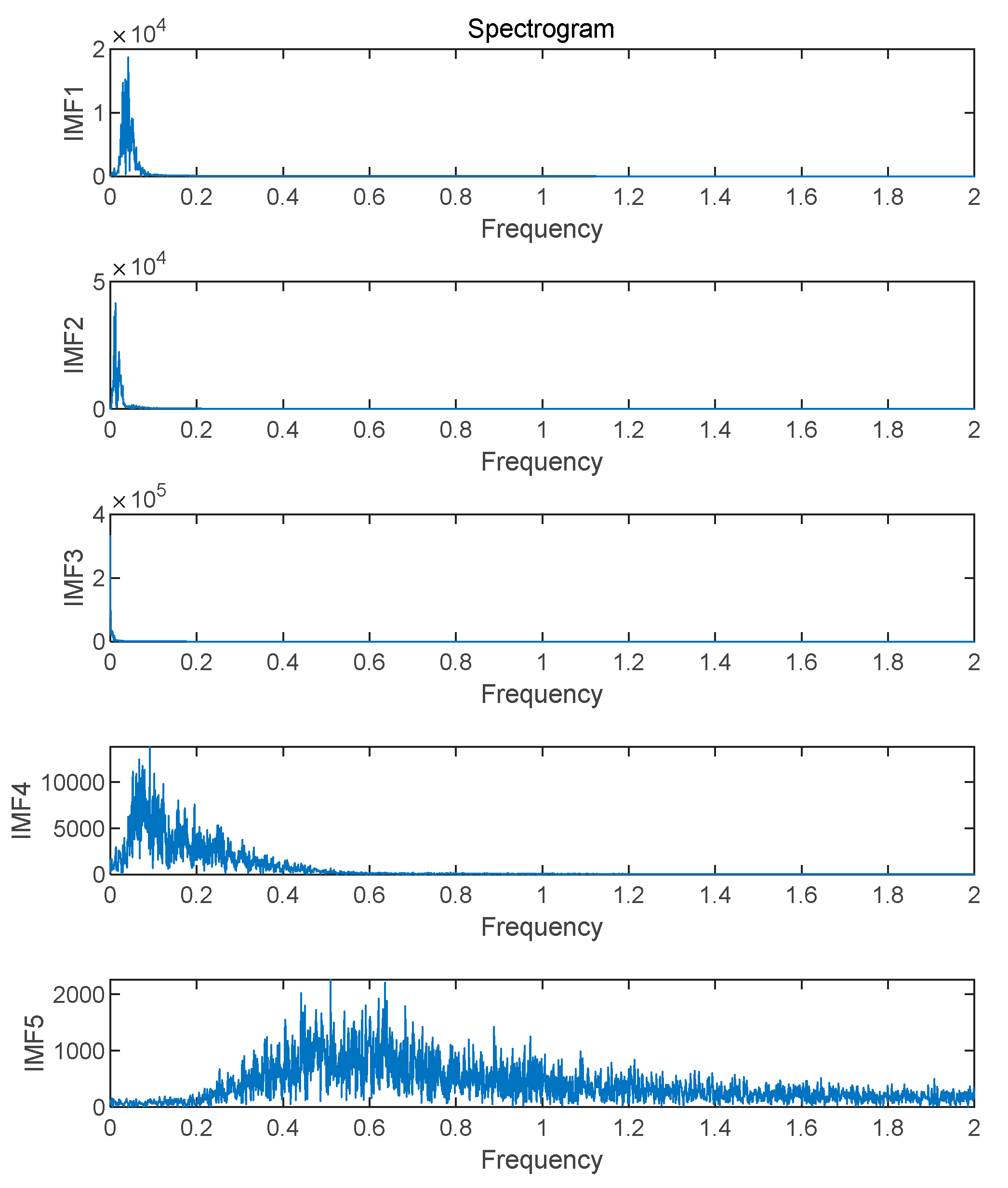
Figure 10.
Forecasting performance of the CEEMDAN-VMD-CNN-BiLSTM model on the training set.
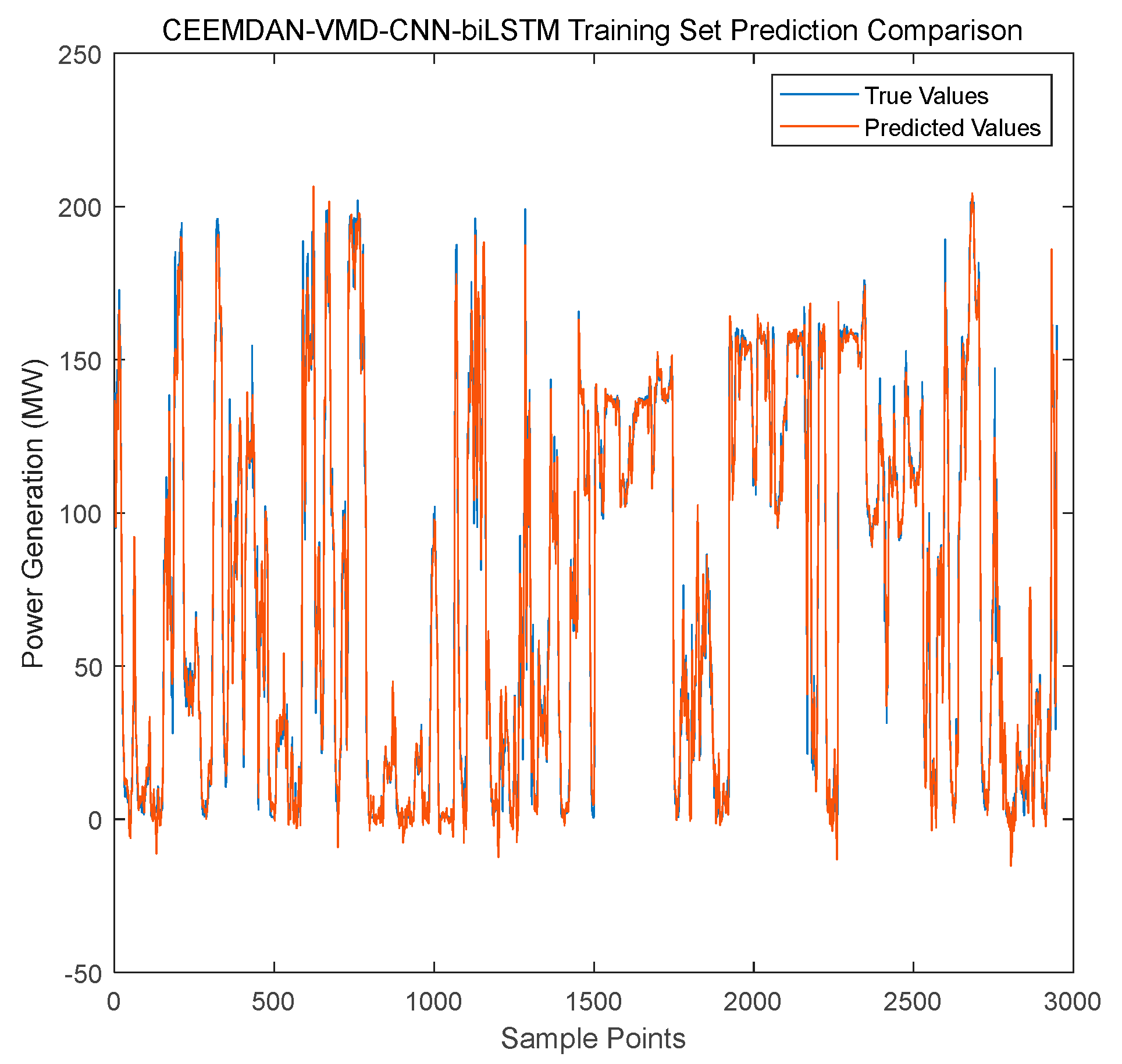
Figure 11.
Forecasting performance of the CEEMDAN-VMD-CNN-BiLSTM model on the test set.
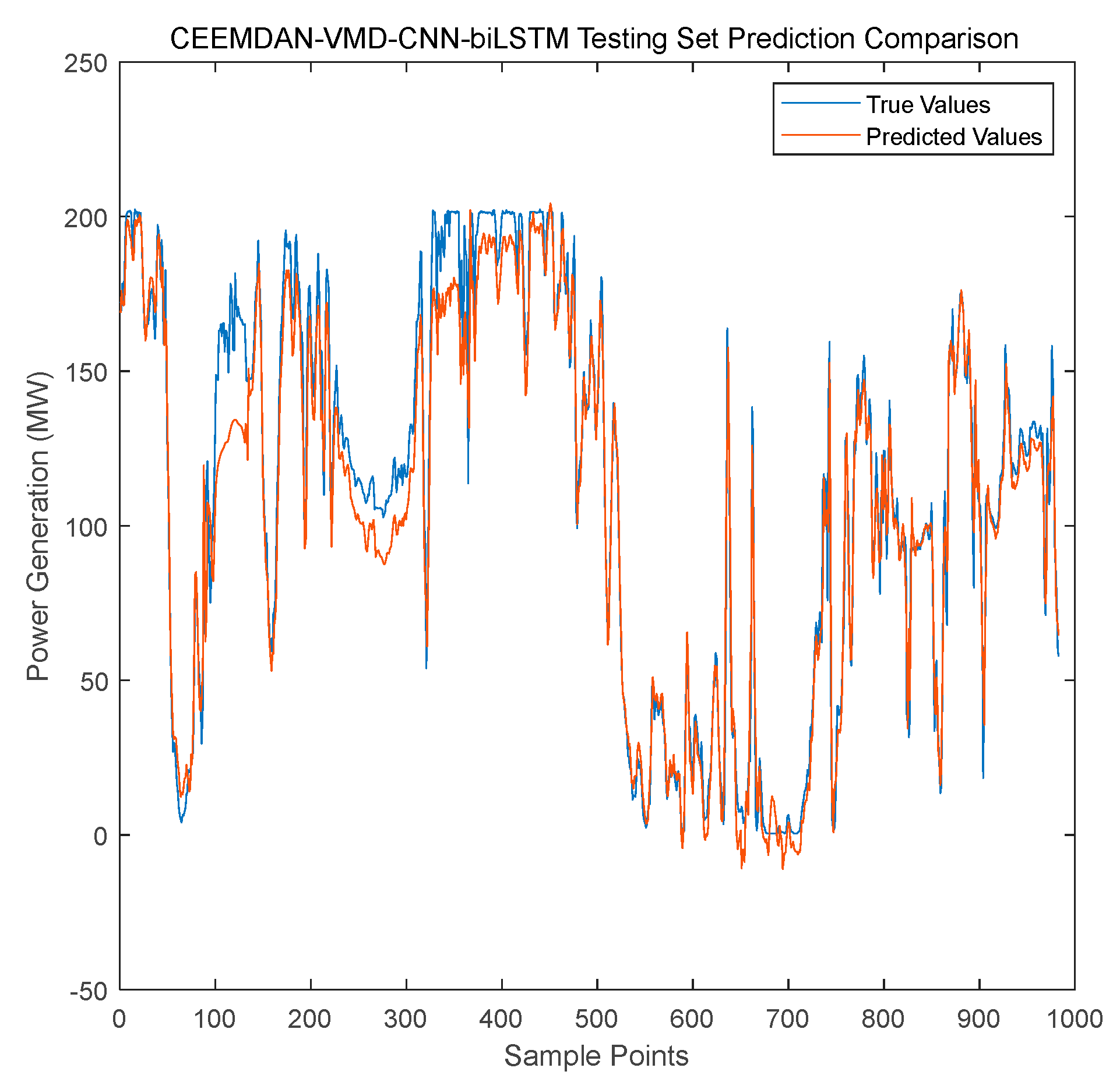
Figure 12.
Forecasting errors of the CEEMDAN-VMD-CNN-BiLSTM model.

Disclaimer/Publisher’s Note: The statements, opinions and data contained in all publications are solely those of the individual author(s) and contributor(s) and not of MDPI and/or the editor(s). MDPI and/or the editor(s) disclaim responsibility for any injury to people or property resulting from any ideas, methods, instructions or products referred to in the content. |
© 2025 by the authors. Licensee MDPI, Basel, Switzerland. This article is an open access article distributed under the terms and conditions of the Creative Commons Attribution (CC BY) license (http://creativecommons.org/licenses/by/4.0/).
Copyright: This open access article is published under a Creative Commons CC BY 4.0 license, which permit the free download, distribution, and reuse, provided that the author and preprint are cited in any reuse.


