
Submitted:
25 April 2025
Posted:
25 April 2025
You are already at the latest version
Abstract
As global energy demand surges, lithium-ion batteries play a pivotal role in enabling renewable energy integration and advancing electrified transportation—both essential for energy independence and environmental sustainability. Their widespread adoption hinges on ensuring long-term reliability, operational resilience, and functional safety. Battery Management Systems (BMS) are central to this mission, requiring accurate internal models for control, monitoring, and diagnostics. Although physics-based models offer interpretability, their computational complexity limits flexibility. Reduced-order models mitigate this, but often lack generalization under dynamic loading. With the growing availability of high-resolution sensor data, data-driven modeling techniques provide a scalable and accurate alternative.
This work investigates learning-based approaches to model battery terminal voltage dynamics using current and historical voltage inputs. We evaluated and compared three architectures: Nonlinear AutoRegressive models with eXogenous inputs (NARX-RNN), Deep Koopman Operator networks that embed nonlinear behavior into latent linear dynamics, and LSTM-based NARX models for temporal pattern learning. The models are trained on experimental datasets and assessed in both steady-state and transient scenarios. Results demonstrate high predictive accuracy and robustness, highlighting their value in BMS development, offline diagnostics, and accelerated testing for safer and more intelligent energy storage systems.
Keywords:
Battery management systems
; Data-driven modeling
; lithium-ion batteries
; NARX-RNN
; LSTM
; machine learning
1. Introduction
Lithium-ion batteries are central to the performance and safety of electric vehicles (EVs) and energy storage systems. Accurate prediction of a battery’s terminal voltage response under dynamic loads is crucial for battery management systems (BMS) to estimate state-of-charge (SOC) and state-of-health (SOH) and to ensure safe operating limits are not exceeded [1]. However, lithium-ion battery dynamics are complex and nonlinear, influenced by electrochemical kinetics, diffusion processes, and aging mechanisms. This has driven the development of a wide spectrum of modeling techniques—each offering trade-offs between physical interpretability, computational complexity, and predictive flexibility.
2. Literature Review
Battery models generally fall into three broad categories: (1) physics-based electrochemical models, (2) reduced-order empirical models like equivalent circuits, and (3) data-driven machine learning models. Each lies at a different point on the spectrum between physical interpretability and ease of deployment. Physics-based models offer insights into internal states and degradation mechanisms but require solving complex PDEs. Empirical models like ECMs offer real-time capability with simplified dynamics. Data-driven models, in contrast, exploit historical cycling data to learn accurate voltage-current mappings without needing explicit physical assumptions.
2.1. Physics-Based Electrochemical Models
Electrochemical models, such as the Doyle-Fuller-Newman (DFN) or pseudo-two-dimensional (P2D) model, provide a physics-grounded framework for simulating lithium-ion battery dynamics [2]. These models capture lithium diffusion in both solid particles and electrolyte phases, enabling accurate predictions of internal states and degradation mechanisms [3]. However, the coupled PDEs make full-order models computationally expensive for real-time use [1].
To reduce complexity, simplified models like the Single Particle Model (SPM) have been proposed, which approximate electrode behavior using a representative spherical particle and uniform electrolyte assumptions [2,3,4]. Advances in solver techniques and computational resources have enabled faster implementations of both full and reduced-order models [3]. These models are widely used in offline parameter identification, virtual dataset generation, and physics-informed benchmarking of data-driven methods [4,5].
2.2. Reduced-Order Models: Equivalent Circuit Models (ECMs)
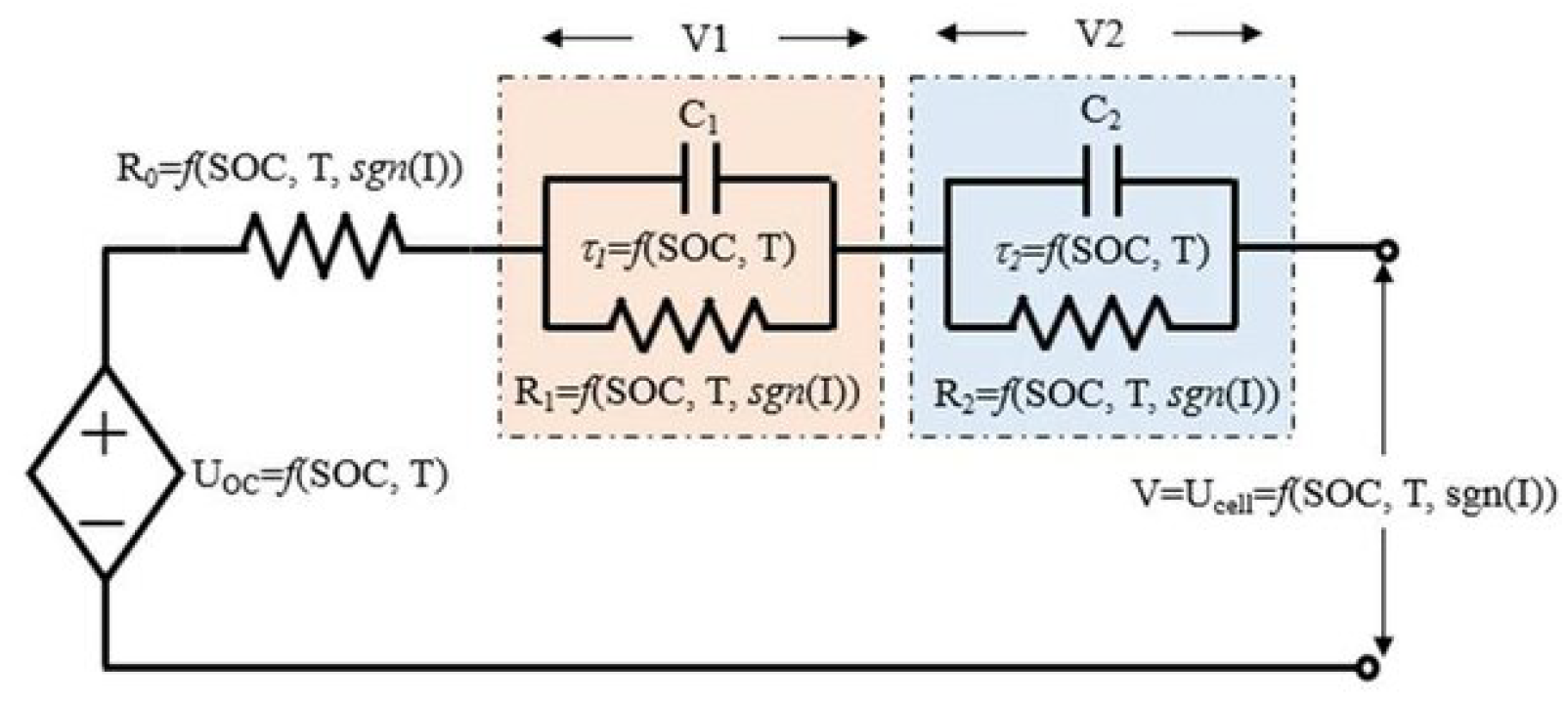
Equivalent Circuit Models (ECMs) replicate terminal voltage response using combinations of resistors, capacitors, and voltage sources, such as in the Thevenin or PNGV configurations [4,7,8]. The ECM model captures open-circuit voltage (OCV) behavior and transient diffusion via RC pairs. While they can achieve low error under well-calibrated conditions, ECMs are empirical by nature and require frequent re-parameterization across aging, temperature, or state-of-health variations [3]. Nonetheless, they remain popular in BMS applications due to their low computational overhead and compatibility with Kalman filtering schemes for SOC estimation [1].
Figure 1.
Schematic of a 2-RC Equivalent Circuit Model (ECM) used to capture lithium-ion battery dynamics [9].
Figure 1.
Schematic of a 2-RC Equivalent Circuit Model (ECM) used to capture lithium-ion battery dynamics [9].
2.3. Data-Driven Modeling Approaches
Data-driven models, in contrast, leverage large volumes of cycling data and neural networks to directly learn voltage-current relationships. These methods prioritize prediction accuracy over interpretability and offer flexibility across operating conditions without needing explicit system identification.
- NARX (Nonlinear Auto-Regressive with eXogenous input) networks use tapped delays of past voltages and currents to regress future voltage [10]. These models can effectively capture dynamics and have been used in voltage prediction and SOC estimation [11,12]. However, they struggle with long-term memory and transients unless hybridized or trained with special loss functions to avoid error accumulation in multi-step predictions.
- Koopman Operator-based methods lift nonlinear dynamics into a latent space with approximately linear evolution. Deep Koopman networks employ autoencoders to discover such coordinates, offering a structured model with interpretable linear dynamics [5,6]. This duality—nonlinear mapping to and from a latent linear system—makes them attractive for both prediction and control [15].
- Hybrid LSTM-NARX approaches combine the autoregressive formulation of NARX type architecture with LSTM’s memory handling [16]. LSTM (Long Short-Term Memory) networks are a class of gated recurrent neural networks capable of learning long-range dependencies [17]. These have shown promise in SOC estimation and direct voltage emulation tasks under dynamic drive cycles [7,8]. LSTMs tend to require large datasets, and their interpretability is limited—making them black-box models from a control perspective. Wei et al. [9,10] showed these hybrids outperform standalone models by shortening gradient propagation paths and better modeling battery behaviors, especially under dynamic conditions.
2.4. Focus of This Work
In this study, we investigate data-driven modeling techniques analyzing three distinct architectures—NARX-RNN, Deep Koopman networks, and LSTM-NARX—using a publicly available dataset based on electric vehicle drive cycle measurements [22]. The objective is to assess their ability to capture terminal voltage dynamics across both steady-state and transient operating regimes while maintaining model simplicity and generalizability.
By “offline” modeling, we refer to training models using complete drive cycle data in a post-processing environment, without constraints on memory or time. These models are designed to be lightweight and interpretable, offering an efficient modeling framework for battery systems without relying on high-fidelity physical models.
The remainder of this paper is organized as follows: Section 3 outlines the underlying battery dynamics motivating data-driven system identification. Section 4, Section 5 and Section 6 describe the architectures of the three modeling approaches. Section 7 details the dataset, implementation, and training setup. Section 8 presents comparative evaluations of model performance across varying operating conditions. Finally, Section 9 summarizes the key findings and outlines potential scope for future research.
3. Battery Dynamical System
The lithium-ion battery can be viewed as a nonlinear dynamical system with the charge/discharge current, temperature as input and terminal voltage as output. The battery’s internal state (related to SoC, electrochemical processes, etc.) governs the relationship between current and voltage, resulting in both instantaneous voltage drops and slower relaxation dynamics [23]. A typical ECM representation is the Thevenin model, consisting of an OCV (open-circuit voltage) source (a static nonlinear function of SoC), an internal resistance causing an immediate voltage jump , and one or more RC pairs to capture transient voltage behavior (diffusion and double-layer effects) [4,11,25]. The continuous-time dynamics for a single RC pair model can be written as:
where is the voltage across the RC network and is the input current (positive for discharge). The terminal voltage then is
neglecting any hysteresis voltage for simplicity. The battery’s state-of-charge evolves with current via (with Q the capacity). Equations (1)–(2) illustrate that battery voltage depends on both the instantaneous input and past inputs (through and q), making it a natural candidate for system identification via autoregressive models.
4. NARX-RNN Model
Nonlinear AutoRegressive models with eXogenous input (NARX) are a class of discrete-time models where the next output is expressed as a nonlinear function of previous outputs and inputs. For battery voltage prediction, a NARX model can be formulated as:
where is a nonlinear mapping and are the chosen output and input memory orders. In a NARX neural network implementation, f is realized by a feedforward neural network (multi-layer perceptron) or an RNN. We use a recurrent neural network architecture for f, effectively creating a NARX-RNN. During training (series mode shown by Figure 2), the actual past voltages are fed as inputs (along with past/current I) to predict , whereas during deployment (parallel mode), the model uses its own previous predictions when true past values are not available [10]. This structure allows the network to learn the battery’s dynamics over a finite memory. One advantage of the NARX-RNN is its simplicity and ability to directly incorporate known exogenous inputs (current) and feedback of past output voltages. It tends to capture static nonlinearities effectively (e.g., the OCV vs SoC relationship) by adjusting the function f accordingly.
5. Deep Koopman Model
The key idea in Deep Koopman Models is to learn an encoder function that maps the observed state (the battery’s measured output ) to a latent state such that the evolution of is linear. Similarly, a decoder maps the latent state back to the output voltage. The dynamical system in the latent space is governed by:
where is the input (battery current at time t), A and B are learned state transition matrices (of dimension and respectively for a d-dimensional latent state), and is the decoder neural network mapping latent state to voltage. In our implementation, h and g are realized as feedforward neural networks (the encoder h takes in the current and voltage at time t and outputs ; the decoder g produces from ). We treat the combination as the overall model mapping from to during training.
Training the Deep Koopman model involves two objectives: (1) reconstruction accuracy - to ensure for all training points and (2) dynamics consistency - to ensure that the latent state evolves approximately according to the linear rule (4). Objective (1) is achieved by using a reconstruction loss for training samples. For objective (2), we include a one-step prediction loss in the latent space: , which penalizes deviations from (4) [5]. The total loss (with a weighting ) is minimized over the training set. The learned matrix A and vector B provide a linear state transition model that approximates the battery’s behavior. This yields interpretability benefits: one can analyze the eigenvalues of A to infer the system’s time constants and stability, or use linear control techniques on the latent state. For example, if A has an eigenvalue close to 1, it suggests a slow-decaying mode (consistent with the slow diffusion voltage recovery in a battery), whereas a small eigenvalue magnitude indicates a fast-decaying transient mode. The decoder g can be understood as capturing the static nonlinear relationship (like the OCV curve) and any measurement mapping.
6. LSTM-NARX Model
Long Short-Term Memory (LSTM) networks are a type of RNN that include gating mechanisms (input, output, and forget gates) to adaptively control the flow of information, which enables learning of both short- and long-term temporal dependencies [12,13]. An LSTM-based model for battery voltage prediction that follows the NARX paradigm of using past values as features is constructed.The LSTM-NARX model leverages the memory capability of recurrent neural networks to predict the terminal voltage of a lithium-ion battery. It follows a nonlinear autoregressive structure, but instead of using fixed tapped delays as in traditional NARX models, it uses an LSTM network to learn temporal dependencies from a sequence of past inputs.
At each time step t, the model receives a window of the past T current inputs:
This sequence is passed through an LSTM network, which processes the data through internal memory and gating mechanisms, capturing both short-term and long-term temporal patterns. The LSTM outputs a voltage increment:
The final predicted terminal voltage is obtained by adding this increment to the previous voltage:
This residual structure improves the network’s ability to learn dynamic trends and prevents bias drift during multi-step predictions. The LSTM gates internally regulate how much of the past is remembered or forgotten at each step, enabling robust prediction even under fast-changing load conditions. Unlike feedforward NARX models, which rely on explicit tapped delays, the LSTM-NARX implicitly learns temporal features without fixed memory windows, making it better suited to capture nonlinear dynamics of the battery across a variety of time scales.
7. Data Generation and Model Architectures
7.1. Data Generation for Training and Testing Datasets
7.2. Training and Testing Datasets
The models were trained using experimental Hybrid Pulse Power Characterization (HPPC) data from a commercial lithium-ion cell [22]. A 2-RC Equivalent Circuit Model (ECM) was also parameterized using the HPPC data and subsequently used to generate synthetic voltage responses by applying persistently exciting input signals, including multi-sine waveforms and sine sweeps at various frequencies. This synthetic dataset complements the experimental HPPC measurements, ensuring that the neural network models are trained on data rich in dynamic behavior and capable of modeling both steady-state and transient battery responses. For testing, we evaluate the model on both steady-state and transient current profiles. The time-series dataset includes input current and terminal voltage sampled at 1 Hz. The cell temperature is within [20-35 degC]. The steady-state region comprises slow charge/discharge cycles with extended constant current periods, allowing the terminal voltage to settle near open-circuit values. The transient region includes dynamic current pulses and step changes from the EPA Urban Dynamometer Driving Schedule (UDDS) profile, exciting the cell’s fast electrochemical dynamics. For neural network training, current and voltage signals were normalized to ensure numerical stability and convergence.
7.3. Model Implementation and Evaluation
All models are implemented using PyTorch and trained via the Adam optimizer. Hyperparameters were tuned by using grid search and validation dataset is used to find the optimal configuration as shown in Table 1.
All models were evaluated using standard metrics:
7.4. Performance Evaluation Metrics
The performance of each model is evaluated using standard error metrics: Root Mean Square Error (RMSE), Mean Absolute Error (MAE), Normalized RMSE (NRMSE), and the coefficient of determination (). These metrics quantify the accuracy of voltage predictions compared to ground-truth measurements:
Here, denotes the ground-truth terminal voltage at time step t, while represents the predicted voltage by the model. is the mean of the actual voltage across the test window, and N is the total number of prediction steps. and are the maximum and minimum values of the actual voltage signal, used for computing the normalized RMSE.
These metrics collectively assess both absolute and relative prediction errors, enabling robust comparison across steady-state and transient regimes.
8. Results and Discussion
Figure 4 shows the measured vs. predicted voltage during the steady-state portion for each model. While all three models manage to track the gradual voltage decline as the battery discharges, the NARX-RNN model’s prediction closely tracks the ground truth in the steady-state region. From the performance metrics, NARX-RNN achieves an RMSE of only 0.0069 V and in the steady-state test (Table 2), outperforming both the Deep Koopman (, ) and LSTM-NARX (, ) models.
Considering the transient regime with rapid current changes as shown in Figure 5, the differences between models become pronounced. The LSTM-NARX model tracks the sharp drop in voltage and the subsequent recovery with remarkable accuracy. The Deep Koopman model captures the general shape but underestimates the voltage dip and recovers more slowly. The NARX-RNN exhibits lag and underpredicts the transient entirely.
The error metrics for the transient case confirm these observations. As shown in Table 3, LSTM-NARX achieves the lowest RMSE of 0.0223 V and . Deep Koopman follows with RMSE 0.0310 V and , while NARX-RNN performs worst with RMSE 0.0490 V and . These results demonstrate the Hybrid LSTM-NARX strength in capturing fast dynamics.
The Koopman model’s intermediate performance in transients suggests that its linear structure captured the dominant time constants but could not fully reproduce nonlinearity.
Regarding stability, NARX-RNN sometimes diverged in long prediction horizons due to error accumulation. Due to their gating and linear state structure, LSTM and Koopman models were more robust in closed loop predictions. Koopman operator’s interpretability, based on its A matrix, also opens doors for control and observer design (e.g., MPC, Kalman filtering), unlike NARX or LSTM which are largely blackbox models.
To summarize the findings:
- Steady-State Accuracy: The NARX-RNN model achieved the highest accuracy in steady-state regions, followed closely by Deep Koopman and LSTM-NARX.
- Transient Accuracy: LSTM-NARX outperformed the others during transient conditions, with Deep Koopman ranking second and NARX-RNN trailing.
- Model Complexity: NARX-RNN had the lowest architectural complexity, followed by Deep Koopman. LSTM-NARX was the most complex due to its recurrent layers and memory mechanisms.
- Interpretability: Deep Koopman provided the most interpretable dynamics through its linear latent space, whereas NARX-RNN and LSTM-NARX behaved as black-box models.
- Prediction Stability: LSTM-NARX and Deep Koopman produced more stable long-horizon predictions, while NARX-RNN exhibited occasional divergence or drift.
These results align with prior findings, such as those by Abbas et al. [30] and Wei et al. [31], where LSTM outperformed simpler architectures in dynamic conditions. Our study extends these insights to include Koopman-based models, highlighting their potential as interpretable yet accurate surrogates of voltage prediction.
9. Conclusions
This work presented a comparative analysis of three machine learning architectures—NARX-RNN, Deep Koopman, and LSTM-NARX—for lithium-ion battery voltage prediction. The models were evaluated under both steady-state and transient conditions using experimentally obtained and synthetically generated datasets enriched with dynamic variations.
- NARX-RNN demonstrated superior accuracy in steady-state conditions, making it well-suited for applications involving slow dynamics and computational constraints.
- LSTM-NARX delivered the best overall performance, particularly excelling in transient regions due to its ability to capture long-term dependencies.
- Deep Koopman offered a favorable balance between accuracy and interpretability by learning latent linear dynamics, making it attractive for control-informed applications.
Each model caters to distinct application needs: NARX-RNN for lightweight deployment, LSTM-NARX for high-fidelity dynamic tracking, and Deep Koopman for interpretable integration with control frameworks.
Future work will explore generalizing these models to incorporate temperature and aging effects for enhanced predictive robustness. Additionally, physics-informed neural networks (PINNs) and hybrid architectures that embed physical constraints will be investigated to reduce model complexity. Such developments are expected to improve both predictive fidelity and the feasibility of deploying data-driven models within embedded BMS.
Abbreviations
| BMS | Battery Management System |
| CNN | Convolutional Neural Network |
| ECM | Equivalent Circuit Model |
| HPPC | Hybrid Pulse Power Characterization |
| LSTM | Long Short-Term Memory |
| Li-ion | Lithium-Ion |
| MAE | Mean Absolute Error |
| ML | Machine Learning |
| MPC | Model Predictive Control |
| NARX | Nonlinear AutoRegressive with eXogenous input |
| NRMSE | Normalized Root Mean Square Error |
| OCV | Open-Circuit Voltage |
| RNN | Recurrent Neural Network |
| RMSE | Root Mean Square Error |
| SOC | State of Charge |
| SOH | State of Health |
| UDDS | Urban Dynamometer Driving Schedule |
References
- Chaturvedi, N.; Yang, R.; Qin, Y.; Krüger, M. Algorithms for advanced battery-management systems. IEEE Control Systems Magazine 2010, 30, 49–68. [Google Scholar] [CrossRef]
- Doyle, M.; Fuller, T.F.; Newman, J. Modeling of Galvanostatic Charge and Discharge of the Lithium/Polymer/Insertion Cell. Journal of The Electrochemical Society 1993, 140, 1526–1533. [Google Scholar] [CrossRef]
- Fotouhi, A.; Auger, D.; Propp, K.; Longo, S.; Foster, M. A Review on Electric Vehicle Battery Modelling: From Lithium-Ion toward Lithium–Sulphur. Renewable and Sustainable Energy Reviews 2016, 56, 1008–1021. [Google Scholar] [CrossRef]
- Chen, M.; Rincón-Mora, G.A. Accurate electrical battery model capable of predicting runtime and I-V performance. IEEE Transactions on Energy Conversion 2006, 21, 504–511. [Google Scholar] [CrossRef]
- Choi, H.; McClintock, R.G.; Subramanian, V.R. Koopman Operator-Based Surrogate Modeling for Lithium-Ion Battery Systems. Journal of The Electrochemical Society 2023, 170, 020541. [Google Scholar] [CrossRef]
- Lusch, B.; Kutz, J.N.; Brunton, S.L. Deep learning for universal linear embeddings of nonlinear dynamics. Nature Communications 2018, 9, 4950. [Google Scholar] [CrossRef]
- Song, Z.; He, H.; Zhang, J.; Ji, C. A hybrid CNN–LSTM model for state of charge estimation of lithium-ion batteries. Journal of Power Sources 2019, 449, 227452. [Google Scholar] [CrossRef]
- Oka, Y.; et al. Battery Emulator Using LSTM for Real-Time Voltage Prediction in EVs. IEEE Transactions on Vehicular Technology 2024, 73, 151–162. [Google Scholar] [CrossRef]
- Wei, Y.; Huang, Y.; Li, J.; Zhang, D. A Hybrid NARX–LSTM Model for Accurate State of Charge Estimation of Lithium-Ion Batteries. Journal of Power Sources 2020, 448, 227400. [Google Scholar] [CrossRef]
- Wei, Y.; Wang, W.; Liu, X. A Hybrid Deep-State Attention Network for Joint SOC and SOH Estimation of Lithium-Ion Batteries. Applied Energy 2023, 345, 120346. [Google Scholar] [CrossRef]
- Plett, G.L. Extended Kalman Filtering for Battery Management Systems of LiPB-Based HEV Battery Packs Part 1. Background. Journal of Power Sources 2004, 134, 252–261. [Google Scholar] [CrossRef]
- Hochreiter, S.; Schmidhuber, J. Long Short-Term Memory. Neural Computation 1997, 9, 1735–1780. [Google Scholar] [CrossRef] [PubMed]
- Greff, K.; Srivastava, R.K.; Koutník, J.; Steunebrink, B.R.; Schmidhuber, J. LSTM: A Search Space Odyssey. IEEE Transactions on Neural Networks and Learning Systems 2017, 28, 2222–2232. [Google Scholar] [CrossRef] [PubMed]
Figure 2.
NARX model during open loop training [26].
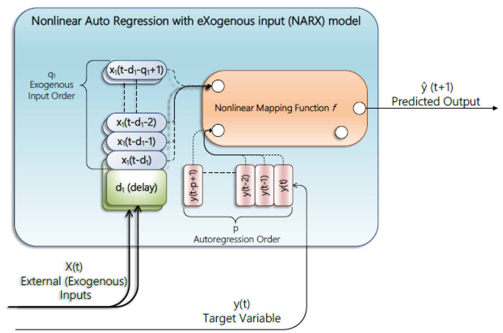
Figure 3.
Deep Koopman operator network architecture[27].
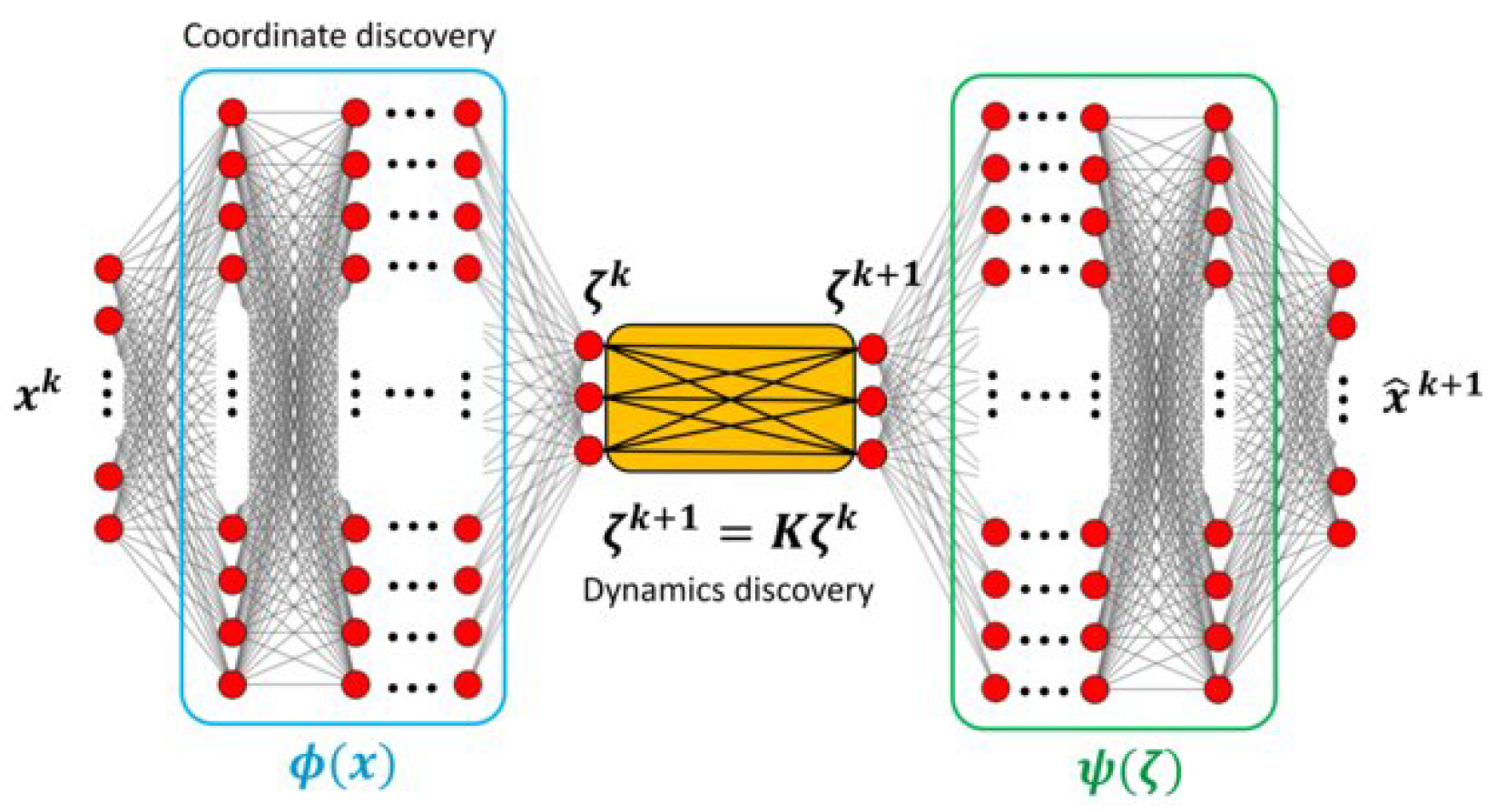
Figure 4.
Steady-state voltage prediction results.
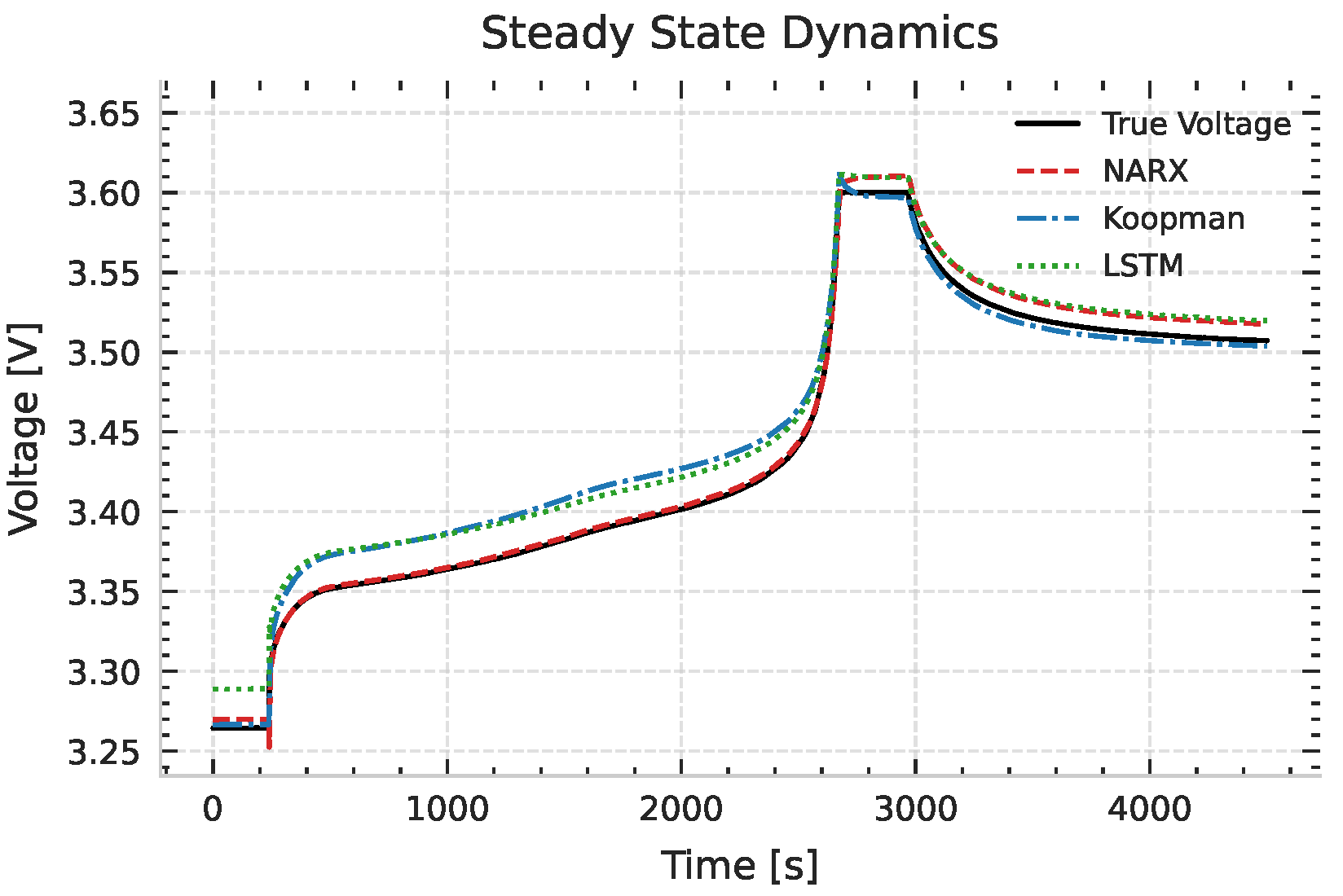
Figure 5.
Transient voltage prediction results.
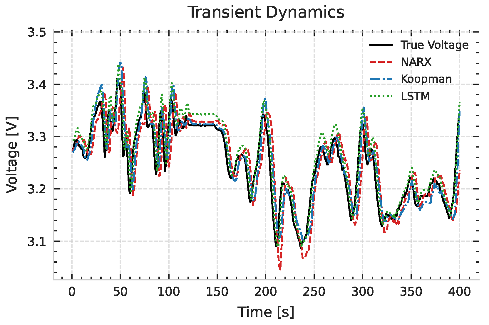

Table 1.
Final Architecture of Implemented Models.
| Model | Architecture Type | Neurons / Layers |
|---|---|---|
| NARX-RNN | RNN + Fully Connected | 32 units, 2 layers |
| Deep Koopman | Encoder–Latent–Decoder (Linear) | 32–4 latent dim–32 |
| LSTM-NARX | LSTM + Residual Skip Connection | 16 units, 1 layer |
Table 2.
Performance Metrics — Steady-State Dynamics.
| Model | RMSE (V) | MAE (V) | NRMSE | |
|---|---|---|---|---|
| NARX-RNN | 0.00690 | 0.00531 | 0.0205 | 0.9941 |
| Deep Koopman | 0.01730 | 0.01423 | 0.0515 | 0.9631 |
| LSTM-NARX | 0.01805 | 0.01734 | 0.0537 | 0.9599 |
Table 3.
Performance Metrics — Transient Dynamics.
| Model | RMSE (V) | MAE (V) | NRMSE | |
|---|---|---|---|---|
| NARX-RNN | 0.04897 | 0.03703 | 0.1515 | 0.5398 |
| Deep Koopman | 0.03101 | 0.02321 | 0.0959 | 0.8155 |
| LSTM-NARX | 0.02225 | 0.01846 | 0.0688 | 0.9050 |
Disclaimer/Publisher’s Note: The statements, opinions and data contained in all publications are solely those of the individual author(s) and contributor(s) and not of MDPI and/or the editor(s). MDPI and/or the editor(s) disclaim responsibility for any injury to people or property resulting from any ideas, methods, instructions or products referred to in the content. |
© 2025 by the authors. Licensee MDPI, Basel, Switzerland. This article is an open access article distributed under the terms and conditions of the Creative Commons Attribution (CC BY) license (http://creativecommons.org/licenses/by/4.0/).
Copyright: This open access article is published under a Creative Commons CC BY 4.0 license, which permit the free download, distribution, and reuse, provided that the author and preprint are cited in any reuse.


