
Submitted:
13 May 2025
Posted:
14 May 2025
You are already at the latest version
Abstract
Accurate modelling of lithium-ion battery degradation is a complex problem, dependent on multiple internal mechanisms that can be affected by a multitude of external conditions. In this study, a transformer-based approach, capable of leveraging historical conditions and known-future inputs is introduced. The model can make predictions from as few as 100 input cycles, and compared to other state-of-the-art techniques our approach shows an increase in accuracy. The model utilises specialised components within its architecture to provide interpretable results, introducing the possibility of understanding path-dependency in Li-Ion battery degradation. The ability to incorporate static metadata opens the door for a foundational deep-learning model for battery degradation forecasting.
Keywords:
lithium-ion batteries
; transformers
; interpretable
; deep learning
1. Introduction
Lithium-ion batteries have emerged as a cornerstone technology across multiple industries worldwide. Notably, they play a crucial role in the rapid advancement of electric vehicles (EV) and large-scale battery energy storage systems (BESS), two sectors that are pivotal to the transition towards sustainable energy solutions. For both of these applications, the associated Battery Management System (BMS) is responsible for optimising battery performance by managing parameters such as voltage, current, and temperature [1]. There is considerable motivation from researchers globally to improve the performance of BMSs [2], as they can extend battery life, reduce failure risks, and mitigate thermal runaway.
EVs rely heavily on efficient battery management to operate safely. The BMS is responsible for several critical functions, including temperature control, cell equalisation, charging and discharging management, and fault analysis. Effective battery state estimation, encompassing the State of Charge (SoC), State of Health (SoH), and Remaining Useful Life (RUL), is vital for ensuring EV safety and performance [3]. Traditional estimation methods, such as the Kalman filter, often lack the adaptability needed to account for battery ageing effects, potentially compromising BMS performance [4].
In addition, BESS are increasingly crucial in efforts to decarbonise the power sector. By facilitating the integration of renewable energy sources into the power grid, BESS also contribute to grid stability and reliability. The BMS is vital to the viability of BESS projects. It is responsible for safety, efficient management of performance, and determining the SoH of batteries. SoH predictions provide crucial information for the maintenance and replacement of batteries. Furthermore, trading strategies for BESS must consider and optimise SoH to balance short-term gains and long-term battery life.
However, the gains generated by BESS through providing flexibility services can be offset by the degradation cost of the lithium-ion batteries. In addition to lifetime and number of cycles, this degradation is sensitive to energy throughput, temperature, SoC, depth of discharge (DoD) and charge/discharge rate (C-rate) [5]. Furthermore, accurate state of health (SoH) estimation is crucial as it dictates the energy throughput, which determines the energy available for trading. This directly impacts the revenue generated from BESS projects and influences key financial metrics such as Levelised Cost of Storage (LCOS) and Internal Rate of Return (IRR), ultimately governing the economic viability of these projects.
A major difficulty for SoH predictions in both EV and BESS applications is the inherent path dependency [6], i.e. the impact of the precise chronological usage of the battery on the SoH. Accounting for path dependency is not inherent to model-based methods – whether they are based on fundamental electrochemical equations [7,8,9] or circuit based equivalent models combined with filtering techniques [10] – because path dependency is still not well understood. Moreover, capturing long-term SoH dependencies on the degradation stress-factors mentioned previously within such frameworks require a large amount of data to be collected over long periods of time, as demonstrated in Ref. [11].
A more efficient approach to SoH prediction is to employ data-driven methods [12] that can store and update key information from degradation data as it becomes available. Traditional data-driven methods for SoH prediction often involve handcrafted feature extraction followed by regression techniques. For instance, Feng et al. [13] used Gaussian process regression (GPR) and polynomial regression to predict SoH and RUL, extracting health indicators from charging current. These methods, while effective, can be time-consuming and labour-intensive, requiring expertise in feature design. Additionally, kernel methods, like support vector machines (SVMs), have been applied for SoH estimation [14]. However, selecting dominant data points can dilute path dependency and reduce prediction accuracy. Neural network (NN) based techniques can be effective because they have an internal state that can represent path information.
The long short-term memory (LSTM) neural network architecture is a popular approach for time-series forecasting due to its ability to capture some long-term dependencies. Zhang et al. [15] studied LSTM based neural networks for SoH predictions. Their results indicated that LSTMs were generally more accurate and precise the SVM based models. More recent studies have focused on end-to-end deep learning approaches using measurement data such as voltage, current, and temperature. Li et al. [16] combined LSTM and CNN networks to separately predict SoH and remaining useful life (RUL) in an end-to-end mode. LSTM models are well-suited for time-series data and can capture some long-term dependencies, which are essential for battery SoH predictions. However, they have limitations such as long training times and a restricted ability to capture very long-term dependencies, which can affect their practical application. This is particularly relevant for SoH prediction as accurate modelling over a large number of cycles is desirable.
Recognising the limitations of LSTM models, researchers have explored more advanced architectures. Cai et al. [17] demonstrated that transformers, when combined with deep neural networks (DNNs), are more effective for battery SoH prediction. The attention mechanism in transformers allows them to assign importance to specific timesteps, thereby capturing long-term dependencies more efficiently than LSTM models. Song et al. [18] further enhanced prediction accuracy by incorporating positional and temporal encoding in transformers to predict battery RUL, addressing the challenge of capturing sequence information.
Zhang et al. [19] integrated an attention layer into a gated residual unit (GRU) architecture, combining it with particle filter information to make accurate RUL predictions. This approach leverages the strengths of both attention mechanisms and traditional filtering techniques, enhancing the robustness of the predictions.
Fan et al. [20] designed a gated recurrent unit-convolutional neural network (GRU-CNN) for direct SoH prediction, which combines the temporal processing capabilities of GRUs with the spatial feature extraction power of CNNs. Gu et al. [21] created a model by combining a CNN and transformer for SoH prediction. The CNN was used to incorporate time-dependent features, whereas the transformer modelled time-independent features. This hybrid approach effectively utilises different neural network architectures to enhance prediction accuracy.
Despite these advancements, previous approaches often struggled with capturing complex dependencies and require extensive computational resources for training. This study presents a novel method for modelling battery degradation and thus sheds light on a critical component of understanding this capability - interpretability of underlying stress factors - using a Temporal Fusion Transformer (TFT) [22]. The TFT model has proven to be more accurate than standard deep-learning approaches for various sequence lengths. It leverages historical conditions and known future inputs to make predictions from as few as 100 input cycles. The model integrates specialised components to provide interpretability, offering insights into path-dependent degradation processes. By incorporating static metadata, our approach provides a robust solution applicable to various battery chemistries and operating conditions. This work aims to enhance the reliability and safety of BMS SoH estimation for EV and BESS applications, providing valuable insights into battery degradation processes and informing optimal management strategies.
In this study, we outline our approach, apply it to a dataset comprising over 100 cells, evaluate its performance relative to other standard neural networks, and demonstrate its potential for interpretability.
2. Framework
2.1. Dataset Description
Severson et al. [23] generated a comprehensive dataset consisting of 124 LFP/graphite cells that were cycled under fast-charging conditions, as shown in Figure 1. The experiments were stopped when the batteries reached end-of-life (EOL) criteria. EOL cycle number ranged from 150 to 2300. This will subsequently be referred to as the “Severson dataset”. The dataset comprises three batches: batch “2017-05-12”, batch “2017-06-30”, and batch “2018-04-12”.
2.2. Evaluation Metrics
For predicting the battery capacity curve, the average mean squared error (MSE) and mean absolute percentage error (MAPE) are calculated across the output sequence. They are defined as:
where and are the true and predicted capacities at the i-th output point, respectively and n is the number of timesteps in the prediction.
2.2.1. Attention
Transformer networks make use of attention, which can be described as mapping vectors consisting of queries (Q) and key-value pairs () to an output. To achieve this, the dot product of query, dimension , is computed with query, dimension . The output of this divided by , before a softmax function is applied to obtain the weights of the values, determining the importance of each value in the input. The matrix of outputs is given by:
To improve the learning capacity of the model, multi-head attention is employed to increase representational power:
where
2.2.2. LSTM Layers
In time-series problems, the location of the data points within the sequence is significant. The TFT leverages local context within sequences through use of an LSTM model, leading to performance improvement in attention-based architectures. This also serves as a replacement for more traditional positional encoding – which makes use of sine and cosine functions which produce a higher dimensional vector that includes information on the location of data within the sequence – by providing an inductive bias for the time ordering of the inputs.
The LSTM encoder is made up of cells that contain the current hidden state. As the information moves through the chain of cells, the hidden state is updated. This is controlled by three internal gates, commonly denoted as input (i), output (o), and forget (f) gates. Each gate multiples the inputs by a weight matrix, adds a bias term, and then applies a sigmoid activation function (). The gates allow the LSTM to effectively either remember or forget different aspects of the input sequence. At time t, the equations describing the LSTM cell and gates are:
where c is the cell state, h is the hidden state, W and U are weight matrices, b is the bias term. The hidden state of the final encoder cell is passed to the next layer in the model.
2.2.3. Variable Selection
The model uses three types of input: past inputs, known future inputs, and static metadata. Each input is initially passed through a variable selection network. This involves transforming the inputs before passing them through a Gated Residual Network (GRN) [22]. Linear transformations are used for continuous variables and entity embeddings [24] are used for the categorical variables. The GRN allows some inputs to skip layers of the network. This enhances the model’s ability to deal with noisy inputs, and prevents the network from becoming too complex. Specifically, the GRN operation is given by:
with the intermediate dense layers and given by:
where is the primary input, is a context vector, is the the Exponential Linear Unit activation function [25].
The variable selection network takes the transformed inputs, represented by , where is the transformed input of the jth variable at time t. is passed into the variable selection network along with an external context vector and the result is multiplied by a softmax function:
is the resulting vector of variable selection weights. This is then used to combine the variables at each time step, by calculating the weighted sum. In this way, the model learns to allocate different importance to each variable. Analysing the learned variable selection weights allows the importance of each variable to be quantified during inference. This is explored further in Section 2.3.
2.3. Interpretability
2.3.1. Temperature Effect
A study of the model’s interpretability is presented in Section 3.4. To do this, test cells which have irregular behaviour in a particular variable are used. Then, the variable importance scores are measured to assess whether the model accounts for that variable’s impact on the degradation. The most obvious choice for this variable is temperature.
The effect of temperature on battery degradation is well studied. The exact implications of operating temperature depend on the dominant ageing mechanism, however, temperatures over generally leads to accelerated ageing, due to increased reaction rates within the cell [26]. The description of temperature dependency of chemical reactions is given by the Arrhenius equation:
where is the activation energy, is the Boltzmann constant, T is the absolute temperature, and A is a pre-exponential factor.
3. Results
To evaluate the model’s performance, a prediction of the cell’s capacity curve was performed. The results are shown in Table 4.
3.1. Variables
The training variables for the model were intentionally selected for ease of calculation, with all continuous variables determined on a per-cycle basis. This approach simplifies the model’s deployment in real-world scenarios. The variables are listed in Table 1.
3.2. Training Procedure
For the experiments, the dataset was partitioned into training, test and validation splits, with five cells reserved for testing, five for validation, and the rest for training. All experiments were run on a single Nvidia V100 GPU. Each epoch took approximately 50 seconds to train and each model was trained for a maximum of 30 epochs. Hyperparameter optimisation was conducted via random search, scanning over a grid of predefined parameters as defined in Table 2:
One test condition is displayed in Section 3.3. Further testing conditions (different permutations of train/test/validation splits) are displayed in Appendix B.
3.3. Model Accuracy Results
The proposed method is compared to a range of conventional data-driven techniques to provide accuracy benchmarks. To do this, the data was split up into the standard train/test/validation groupings. 18 cells were reserved for testing, 18 for validation, and the remainder were used for training. Early stopping was used to avoid overtraining. Three different permutations of train/test/validation were tested in total (results for the last two are presented in Appendix B). To assess the ability of the model to perform over a variety of context windows, three different combinations of varying input/output length were chosen. The details of each experiment are summarised in Table 3.
Interestingly, as the input length increased from 100 cycles to 200 cycles (while keeping the output length fixed at 400), both the MAPE and MSE worsened, indicating a decrease in performance. Several factors may explain this. First, the LSTM input encoder and self-attention layers, which have a complexity of with respect to input length [27], may cause bottlenecks during training. Second, this suggests that the most recent input timesteps are generally more influential. The model may become “distracted” by earlier timesteps, leading to overfitting and decreased accuracy as the input length grows.
However, as shown in Table 5, when the output length was increased to 600 cycles, the model outputs remained accurate compared to the benchmarks.
When evaluated using the Severson dataset, the model demonstrates substantial performance improvements. Unlike purely physics-based methods, the model does not require any prior electrochemical knowledge of the battery cell. Additionally, by incorporating battery type and capacity as static inputs (metadata), the model enables the training of a generalized model on datasets that include degradation data from various cells. This allows the model to leverage shared knowledge from similar degradation patterns across different cells. An example of the model’s capacity prediction for one cell is shown in Figure 2.

Table 4.
Performance comparison of different models using 100 Input Cycles and 400 Output Cycles
| Model | MAPE | MSE |
|---|---|---|
| CNN | 1.12 | 2.82 |
| LSTM | 1.38 | 3.84 |
| Transformer | 1.43 | 3.95 |
| Our model | 0.67 | 1.52 |
Table 5.
Performance comparison of different models using 200 Input Cycles and 400 Output Cycles
| Model | MAPE | MSE |
|---|---|---|
| CNN | 0.87 | 1.73 |
| LSTM | 0.87 | 2.07 |
| Transformer | 1.02 | 2.54 |
| Our model | 0.37 | 0.41 |
Table 6.
Performance comparison of different models using 200 Input Cycles and 600 Output Cycles
| Model | MAPE | MSE |
|---|---|---|
| CNN | 0.89 | 1.86 |
| LSTM | 1.02 | 2.07 |
| Transformer | 1.40 | 3.35 |
| Our model | 0.68 | 1.83 |
Table 7.
Performance comparison of different models
| Model | 100I, 400O | 200I, 400O | 200I, 600O | |||
|---|---|---|---|---|---|---|
| MAPE | MAE | MAPE | MAE | MAPE | MAE | |
| CNN | 1.12 | 2.82 | 0.87 | 1.73 | 0.89 | 1.86 |
| LSTM | 1.38 | 3.84 | 0.87 | 2.07 | 1.02 | 2.07 |
| Transformer | 1.43 | 3.95 | 1.02 | 2.54 | 1.40 | 3.35 |
| Our model | 0.67 | 1.52 | 0.37 | 0.41 | 0.68 | 1.83 |
3.4. Interpretability
Having established the accuracy of the model, we now demonstrate how relationships between the data that lead to predictions can be interpreted. While some conventional data-driven techniques can produce accurate results, the relative contributions of each the potentially many features to the overall degradation remain unknown. Variable selection networks on both static and time-dependent covariates, quantifying the impact of each feature per instance and filtering out unnecessary, noisy inputs.
The Severson dataset can be used to investigate the usefulness of the model’s variable importance scores. To do this, outlier cells in specific variables were used. For example, a cell with a relatively high charging temperature could be used as it is expected that the degradation of this cell would be more strongly affected by the charging temperature compared with an average cell. By calculating the variable importance score for this cell and comparing it with the average scores across the dataset, we can assess the model’s ability to make realistic estimates. If the charging temperature’s importance score for the test cell exceeds the average, it suggests that the model accurately reflects the relative importance of this variable.
Figure 3 shows the variable importance weights for the whole Severson dataset. As expected, the cycle number, i.e. the age of the cell, is the most important factor affecting the degradation. The 2nd and 3rd most important variables are both temperature variables, which is also sensible.
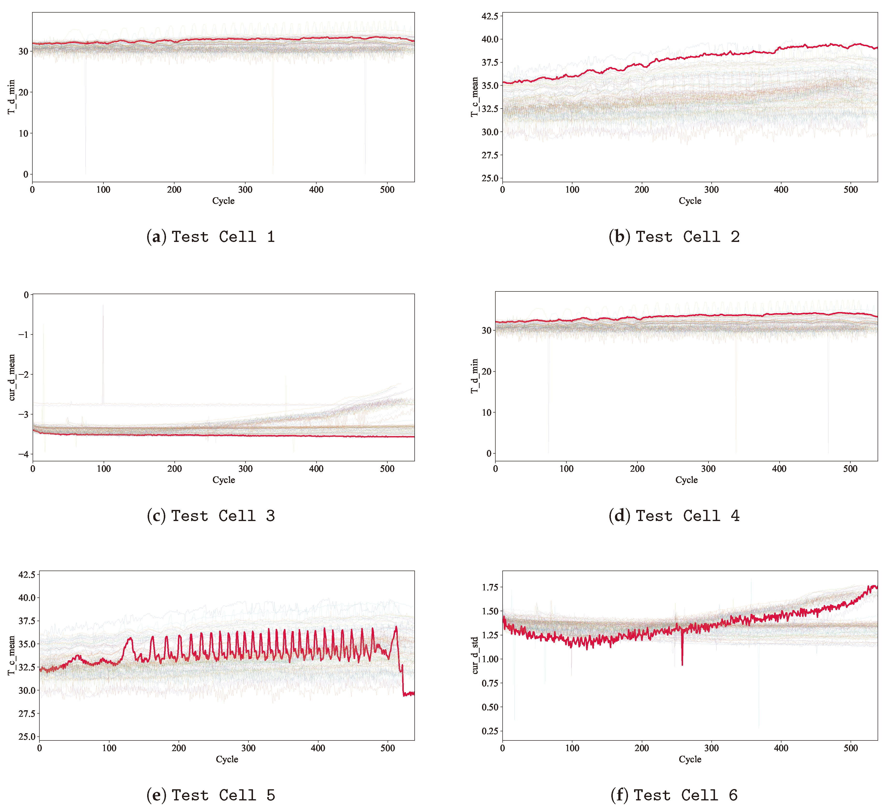
Several test cases have been identified for studying the variable importances. Here we present test cell 1 as an example and others are shown in the Appendix. The charging temperature for this cell is much higher than average, as shown in Figure 4. The corresponding attention scores for this cell are shown in Figure 5. Comparing this with Figure 3 demonstrates that the test cell has a higher attention score for the mean charging temperature (labelled T_c_mean) than the average score for the whole dataset. The cell’s attention score for this variable was 5.48%, making it the 5th most important variable; whereas the average score was 4.79%, which ranks as the 8th most important variable. In this way, the model can correctly assign a higher importance where a particular feature plays a greater role in the cell’s degradation.
4. Conclusions
This study has presented a novel approach for modelling battery degradation using a Temporal Fusion Transformer. The proposed model has demonstrated superior accuracy compared to standard deep-learning methods across various sequence lengths. The mean absolute error for the predicted capacity curve was found to be between 0.67% and 0.85%, compared with 0.87% – 1.40% for the benchmark models.
The model effectively integrates both continuous and categorical inputs, which can be either static or time-varying. In addition, it offers interpretable outputs, yielding valuable insights into specific factors that impact a given battery’s degradation. This could enable a user to extend the life of a battery during operation. Moreover, the model is capable of accurately forecasting degradation curves with as few as 100 input cycles.
The model presented in this study has great potential to enhance the reliability and safety of lithium-ion batteries in electric vehicles or energy storage systems.
Funding
This research received no external funding.
Data Availability Statement
The dataset used in this study are publicly available at https://data.matr.io/1/
Acknowledgments
We express our gratitude to Envision Energy for supplying the R&D resources that made this work possible.
Conflicts of Interest
The authors declare no conflicts of interest
Appendix A. Additional Variable Importance Results
Figure 3 shows the average attention weights over the whole dataset. Section 3.4 showed an example of a cell with a high charging temperature and a correspondingly high attention score for that variable. Other examples are shown below:
Table A1.
Additional test cells for variable importance study. The importance score for the chosen variable is shown along with the average importance score for that variable over the whole dataset.
Table A1.
Additional test cells for variable importance study. The importance score for the chosen variable is shown along with the average importance score for that variable over the whole dataset.
Figure A1.
The six test cells used for the variable importance study are shown. For each cell, the particular variable is plotted with the test cell shown as a red line and the other cells in the sample shown as lighter coloured lines. This demonstrates that each test cell is an outlier in its respective variable.
Appendix B. Additional Accuracy Results
Accuracy results from other permutations of train/test splits.
Appendix B.1. Test Condition 2
Table A2.
Comparison of results of various approaches using 100 Input Cycles and 400 Output Cycles—Test Condition 2
Table A2.
Comparison of results of various approaches using 100 Input Cycles and 400 Output Cycles—Test Condition 2
| Model | MAPE | MSE |
|---|---|---|
| CNN | 1.27 | 4.08 |
| LSTM | 1.81 | 5.94 |
| Transformer | 1.75 | 5.37 |
| Our model | 0.65 | 1.40 |
Table A3.
Comparison of results of various approaches using 200 Input Cycles and 400 Output Cycles—Test Condition 2
Table A3.
Comparison of results of various approaches using 200 Input Cycles and 400 Output Cycles—Test Condition 2
| Model | MAPE | MSE |
|---|---|---|
| CNN | 1.01 | 2.36 |
| LSTM | 1.24 | 3.76 |
| Transformer | 1.22 | 3.74 |
| Our model | 0.75 | 1.49 |
Table A4.
Comparison of results of various approaches using 200 Input Cycles and 600 Output Cycles—Test Condition 2
Table A4.
Comparison of results of various approaches using 200 Input Cycles and 600 Output Cycles—Test Condition 2
| Model | MAPE | MSE |
|---|---|---|
| CNN | 1.10 | 2.99 |
| LSTM | 1.26 | 3.04 |
| Transformer | 1.43 | 3.25 |
| Our model | 0.67 | 0.71 |
Appendix B.2. Test Condition 3
Table A5.
Comparison of results of various approaches using 100 Input Cycles and 400 Output Cycles—Test Condition 3
Table A5.
Comparison of results of various approaches using 100 Input Cycles and 400 Output Cycles—Test Condition 3
| Model | MAPE | MSE |
|---|---|---|
| CNN | 1.29 | 4.21 |
| LSTM | 1.73 | 5.30 |
| Transformer | 1.21 | 3.40 |
| Our model | 0.84 | 1.46 |
Table A6.
Comparison of results of various approaches using 200 Input Cycles and 400 Output Cycles—Test Condition 3
Table A6.
Comparison of results of various approaches using 200 Input Cycles and 400 Output Cycles—Test Condition 3
| Model | MAPE | MSE |
|---|---|---|
| CNN | 1.14 | 3.52 |
| LSTM | 1.22 | 3.57 |
| Transformer | 1.17 | 2.32 |
| Our model | 0.57 | 1.29 |
Table A7.
Comparison of results of various approaches using 200 Input Cycles and 600 Output Cycles—Test Condition 3
Table A7.
Comparison of results of various approaches using 200 Input Cycles and 600 Output Cycles—Test Condition 3
| Model | MAPE | MSE |
|---|---|---|
| CNN | 1.16 | 3.11 |
| LSTM | 1.22 | 3.19 |
| Transformer | 1.13 | 2.90 |
| Our model | 0.71 | 2.62 |
References
- Liu, Q.; Chen, G. Design of Electric Vehicle Battery Management System. J. Phys.: Conf. Ser. 2023, 2614, 012001. [Google Scholar] [CrossRef]
- Habib, A.K.M.A.; Hasan, M.K.; Issa, G.F.; Singh, D.; Islam, S.; Ghazal, T.M. Lithium-Ion Battery Management System for Electric Vehicles: Constraints, Challenges, and Recommendations. Batteries 2023, 9, 152. [Google Scholar] [CrossRef]
- Kassim, M.R.M.; Jamil, W.A.W.; Sabri, R.M. State-of-Charge (SOC) and State-of-Health (SOH) Estimation Methods in Battery Management Systems for Electric Vehicles. In Proceedings of the 2021 IEEE International Conference on Computing (ICOCO); 2021; pp. 91–96. [Google Scholar] [CrossRef]
- Barré, A.; Deguilhem, B.; Grolleau, S.; Gérard, M.; Suard, F.; Riu, D. A Review on Lithium-Ion Battery Ageing Mechanisms and Estimations for Automotive Applications. J. Power Sources 2013, 241, 680–689. [Google Scholar] [CrossRef]
- Uddin, K.; Perera, S.; Widanage, W.D.; Somerville, L.; Marco, J. Characterising Lithium-Ion Battery Degradation through the Identification and Tracking of Electrochemical Battery Model Parameters. Batteries 2016, 2, 13. [Google Scholar] [CrossRef]
- Mowri, S.; Barai, A.; Moharana, S.; Gupta, A.; Marco, J. Assessing the Impact of First-Life Lithium-Ion Battery Degradation on Second-Life Performance. Energies 2024, 17, 501. [Google Scholar] [CrossRef]
- Lin, W.-J.; Chen, K.-C. Evolution of Parameters in the Doyle-Fuller-Newman Model of Cycling Lithium-Ion Batteries by Multi-Objective Optimization. Appl. Energy 2022, 314, 118925. [Google Scholar] [CrossRef]
- Dubarry, M.; Beck, D. Perspective on Mechanistic Modeling of Li-Ion Batteries. Acc. Mater. Res. 2022, 3, 843–853. [Google Scholar] [CrossRef]
- Uddin, K.; Somerville, L.; Barai, A.; Lain, M.; Ashwin, T.; Jennings, P.; Marco, J. The Impact of High-Frequency-High-Current Perturbations on Film Formation at the Negative Electrode-Electrolyte Interface. Electrochim. Acta 2017, 233, 1–12. [Google Scholar] [CrossRef]
- Dong, H.; Jin, X.; Lou, Y.; Wang, C. Lithium-Ion Battery State of Health Monitoring and Remaining Useful Life Prediction Based on Support Vector Regression-Particle Filter. J. Power Sources 2014, 271, 114–123. [Google Scholar] [CrossRef]
- Vetter, J.; Novák, P.; Wagner, M.; Veit, C.; Möller, K.-C.; Besenhard, J.; Winter, M.; Wohlfahrt-Mehrens, M.; Vogler, C.; Hammouche, A. Ageing Mechanisms in Lithium-Ion Batteries. J. Power Sources 2005, 147, 269–281. [Google Scholar] [CrossRef]
- Li, X.; Ju, L.; Geng, G.; Jiang, Q. Data-Driven State-of-Health Estimation for Lithium-Ion Battery Based on Aging Features. Energy 2023, 274, 127378. [Google Scholar] [CrossRef]
- Feng, H.; Shi, G. SOH and RUL Prediction of Li-Ion Batteries Based on Improved Gaussian Process Regression. J. Power Electron. 2021, 21, 1845–1854. [Google Scholar] [CrossRef]
- Feng, R.; Wang, S.; Yu, C.; Hai, N.; Fernandez, C. High Precision State of Health Estimation of Lithium-Ion Batteries Based on Strong Correlation Aging Feature Extraction and Improved Hybrid Kernel Function Least Squares Support Vector Regression Machine Model. J. Energy Storage 2024, 90, 111834. [Google Scholar] [CrossRef]
- Zhang, Y.; Xiong, R.; He, H.; Pecht, M.G. Long Short-Term Memory Recurrent Neural Network for Remaining Useful Life Prediction of Lithium-Ion Batteries. IEEE Trans. Veh. Technol. 2018, 67, 5695–5705. [Google Scholar] [CrossRef]
- Li, P.; Zhang, Z.; Grosu, R.; Deng, Z.; Hou, J.; Rong, Y.; Wu, R. An End-to-End Neural Network Framework for State-of-Health Estimation and Remaining Useful Life Prediction of Electric Vehicle Lithium Batteries. Renew. Sustain. Energy Rev. 2022, 156, 111843. [Google Scholar] [CrossRef]
- Cai, Y.; Li, W.; Zahid, T.; Zheng, C.; Zhang, Q.; Xu, K. Early Prediction of Remaining Useful Life for Lithium-Ion Batteries Based on CEEMDAN-Transformer-DNN Hybrid Model. Heliyon 2023, 9, e17754. [Google Scholar] [CrossRef] [PubMed]
- Song, W.; Wu, D.; Shen, W.; Boulet, B. A Remaining Useful Life Prediction Method for Lithium-Ion Battery Based on Temporal Transformer Network. Procedia Comput. Sci. 2023, 217, 1830–1838. [Google Scholar] [CrossRef]
- Zhang, J.; Huang, C.; Chow, M.-Y.; Li, X.; Tian, J.; Luo, H.; Yin, S. A Data-Model Interactive Remaining Useful Life Prediction Approach of Lithium-Ion Batteries Based on PF-BiGRU-TSAM. IEEE Trans. Ind. Inform. 2024, 20, 1144–1154. [Google Scholar] [CrossRef]
- Fan, Y.; Xiao, F.; Li, C.; Yang, G.; Tang, X. A Novel Deep Learning Framework for State of Health Estimation of Lithium-Ion Battery. J. Energy Storage 2020, 32, 101741. [Google Scholar] [CrossRef]
- Gu, X.; See, K.; Li, P.; Shan, K.; Wang, Y.; Zhao, L.; Lim, K.C.; Zhang, N. A Novel State-of-Health Estimation for the Lithium-Ion Battery Using a Convolutional Neural Network and Transformer Model. Energy 2023, 262, 125501. [Google Scholar] [CrossRef]
- Lim, B.; Arık, S.Ö.; Loeff, N.; Pfister, T. Temporal Fusion Transformers for Interpretable Multi-Horizon Time Series Forecasting. Int. J. Forecast. 2021, 37, 1748–1764. [Google Scholar] [CrossRef]
- Severson, K.A.; Attia, P.M.; Jin, N.; Perkins, N.; Jiang, B.; Yang, Z.; Chen, M.H.; Aykol, M.; Herring, P.K.; Fraggedakis, D.; et al. Data-Driven Prediction of Battery Cycle Life Before Capacity Degradation. Nat. Energy 2019, 4, 383–391. [Google Scholar] [CrossRef]
- Gal, Y.; Ghahramani, Z. A Theoretically Grounded Application of Dropout in Recurrent Neural Networks. In Advances in Neural Information Processing Systems; Lee, D., Sugiyama, M., Luxburg, U., Guyon, I., Garnett, R., Eds.; Curran Associates, Inc.: 2016; Vol. 29. https://proceedings.neurips.cc/paper_files/paper/2016/file/076a0c97d09cf1a0ec3e19c7f2529f2b-Paper.pdf.
- Clevert, D.-A.; Unterthiner, T.; Hochreiter, S. Fast and Accurate Deep Network Learning by Exponential Linear Units (ELUs). arXiv 2015, arXiv:1511.07289. [Google Scholar]
- Kucinskis, G.; Bozorgchenani, M.; Feinauer, M.; Kasper, M.; Wohlfahrt-Mehrens, M.; Waldmann, T. Arrhenius Plots for Li-Ion Battery Ageing as a Function of Temperature, C-Rate, and Ageing State–An Experimental Study. J. Power Sources 2022, 549, 232129. [Google Scholar] [CrossRef]
- Vaswani, A.; Shazeer, N.; Parmar, N.; Uszkoreit, J.; Jones, L.; Gomez, A.N.; Kaiser, Ł.; Polosukhin, I. Attention Is All You Need. Adv. Neural Inf. Process. Syst. 2017, 30. [Google Scholar]
Figure 1.
Capacity curves for the cells in the Severson dataset.
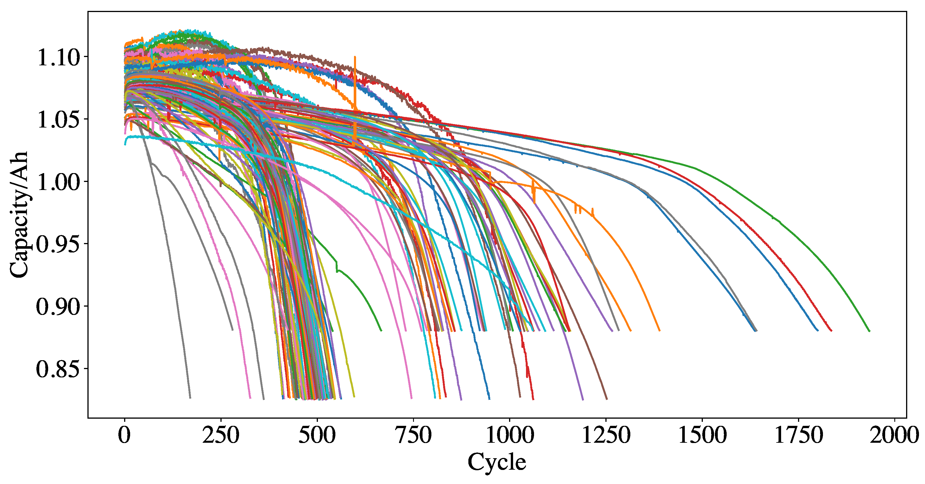
Figure 2.
Predicted capacity from the trained TFT for 400 cycles of one cell, using 100 input cycles. The mean absolute error for the prediction is displayed.
Figure 2.
Predicted capacity from the trained TFT for 400 cycles of one cell, using 100 input cycles. The mean absolute error for the prediction is displayed.
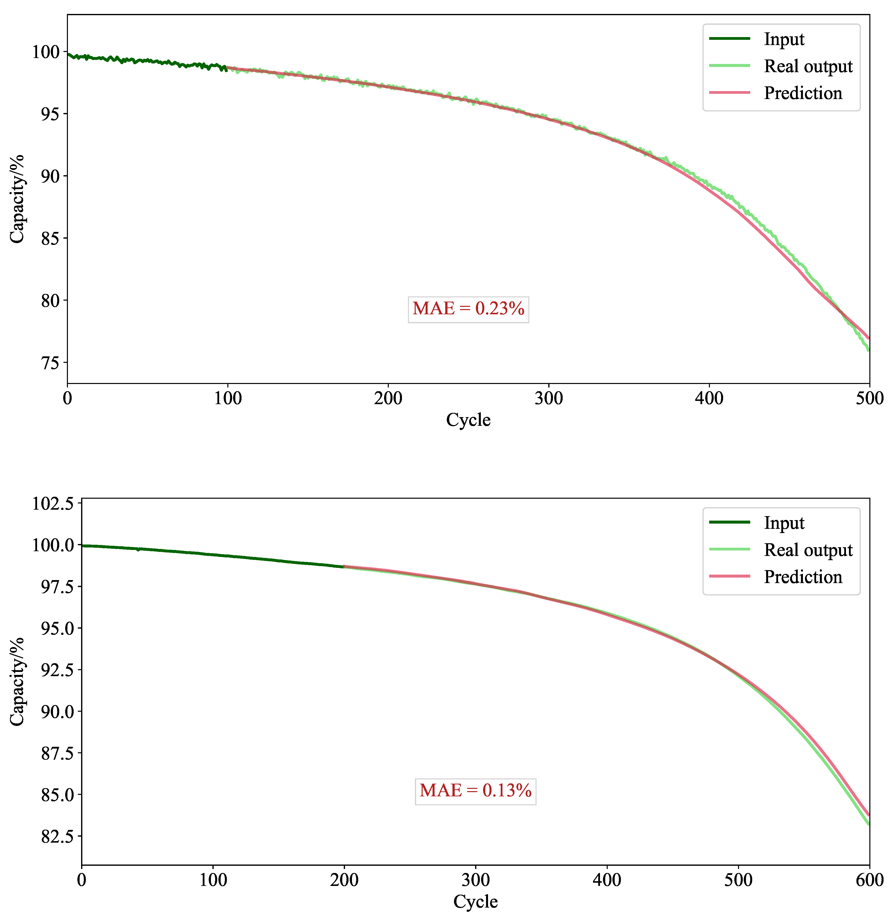
Figure 3.
Average variable importance weights for all cells.
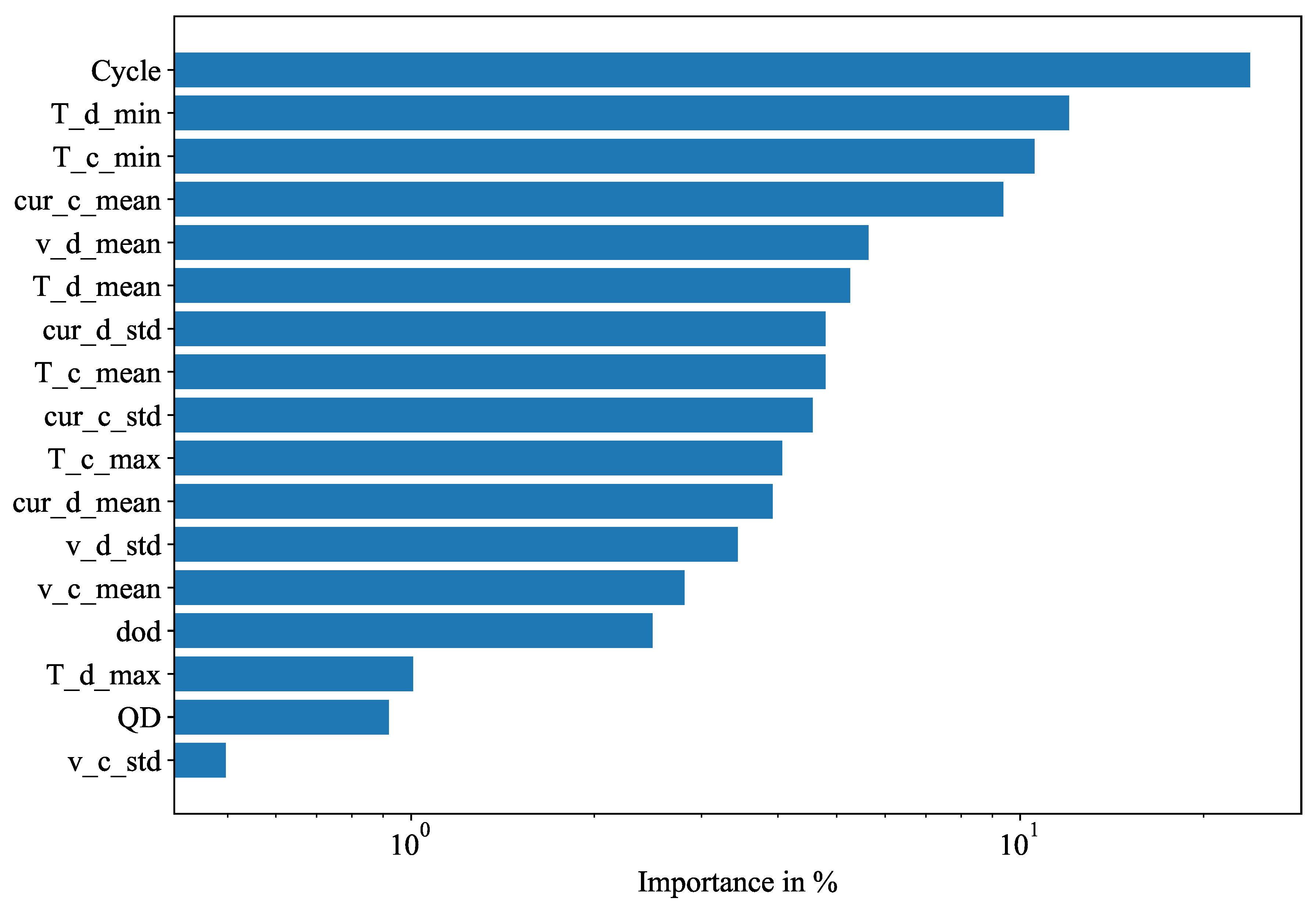
Figure 4.
Minimum charging temperature for cell test cell 2 (red line) compared with all other cells in the dataset, showing that the chosen cell is higher than average in this variable.
Figure 4.
Minimum charging temperature for cell test cell 2 (red line) compared with all other cells in the dataset, showing that the chosen cell is higher than average in this variable.
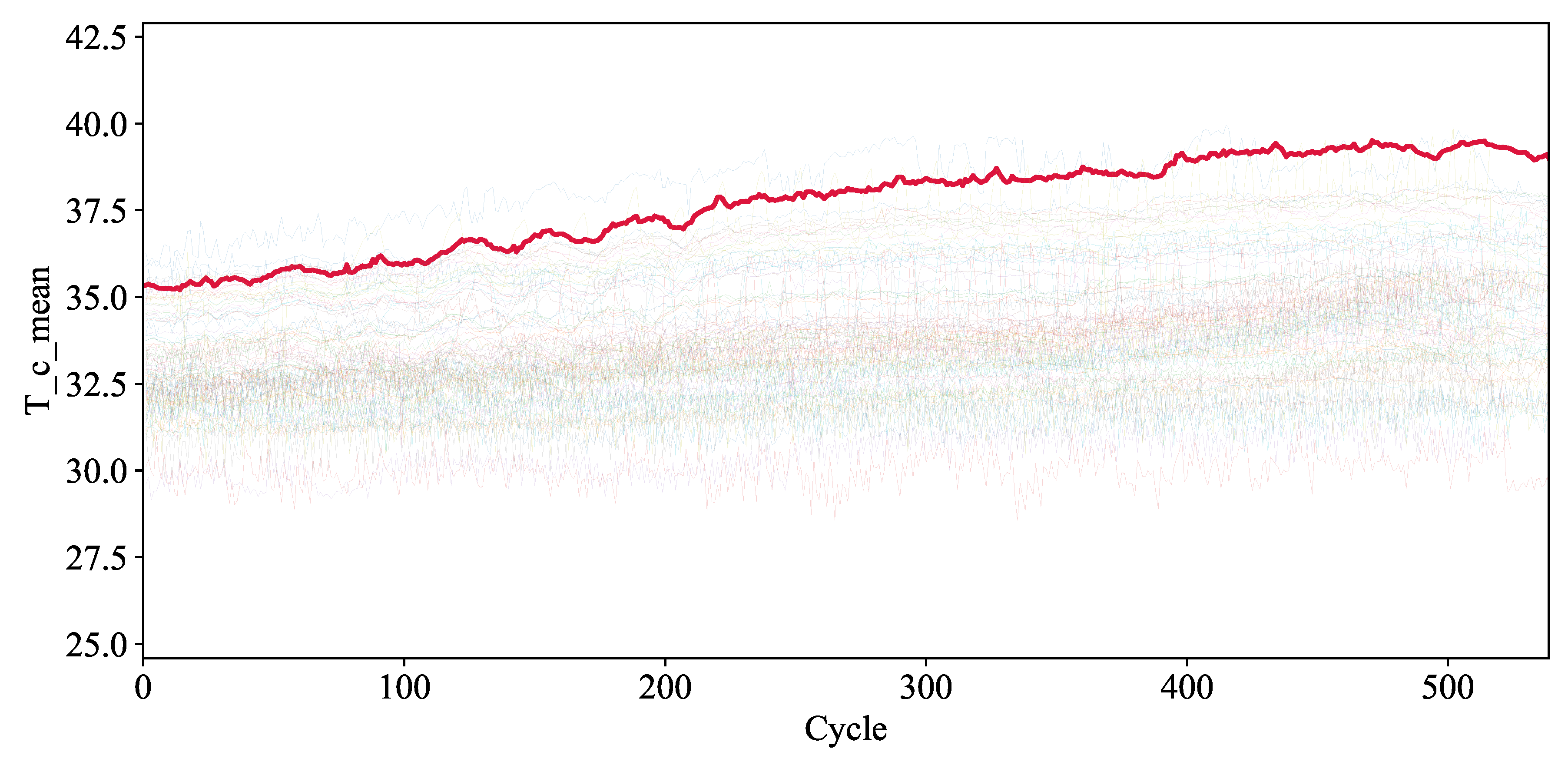
Figure 5.
Variable importance weights for test cell 2
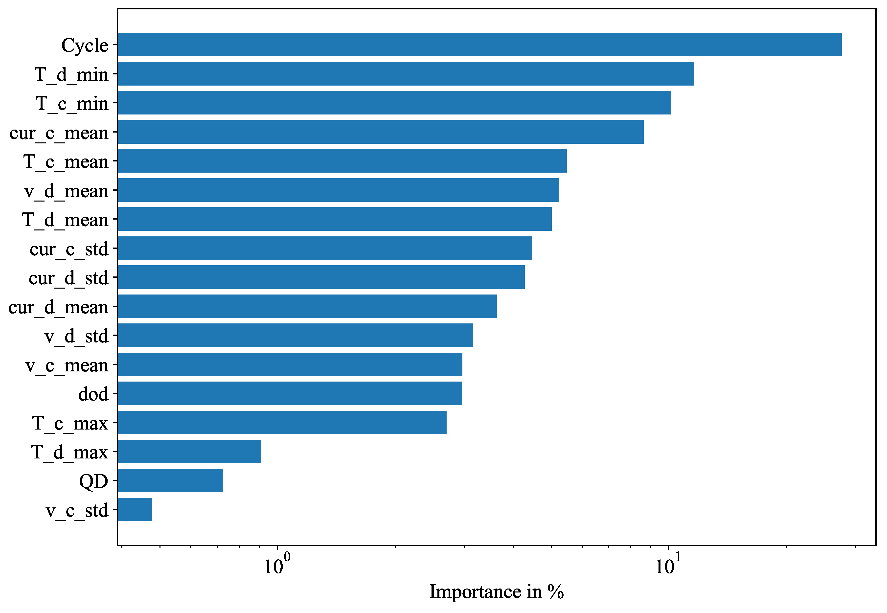
Table 1.
List of variables used in the TFT training.
| Variable Description | Name | Type |
|---|---|---|
| Cycle number | Cycle | Timestep |
| Current capacity | QD | Continuous, input |
| Future capacity | QD_target | Continuous, target |
| Battery | Battery | Categorical, input |
| Average charging voltage | v_c_mean | Continuous, input |
| Average discharging voltage | v_d_mean | Continuous, input |
| Standard deviation of charging voltage | v_c_std | Continuous, input |
| Standard deviation of discharging voltage | v_d_std | Continuous, input |
| Depth of discharge | dod | Continuous, input |
| Average charging current | cur_c_mean | Continuous, input |
| Average discharging current | cur_d_mean | Continuous, input |
| Standard deviation of charging current | cur_c_std | Continuous, input |
| Standard deviation of discharging current | cur_d_std | Continuous, input |
| Average charging temperature | T_c_mean | Continuous, input |
| Average discharging temperature | T_d_mean | Continuous, input |
| Standard deviation of charging temperature | T_c_std | Continuous, input |
| Standard deviation of discharging temperature | T_d_std | Continuous, input |
| Minimum charging temperature | T_c_min | Continuous, input |
| Minimum discharging temperature | T_d_min | Continuous, input |
| Maximum charging temperature | T_c_max | Continuous, input |
| Maximum discharging temperature | T_d_max | Continuous, input |
Table 2.
Search values for each hyperparameter used in the optimisation.
| Hyperparameter | Values |
|---|---|
| Dropout rate | [0.1, 0.2, 0.3, 0.4, 0.5, 0.7, 0.9] |
| Hidden Layer Size | [10, 20, 40, 80] |
| Minibatch size | [64, 128, 256] |
| Learning rate | [0.0001, 0.001, 0.01] |
| Max. gradient norm | [0.01, 1.0, 100.0] |
| Num. heads | [1, 4] |
Table 3.
Input and output sequence length configurations for each permutation setting.
| Permutation | Input Length | Output Length |
|---|---|---|
| 1 | 100 | 400 |
| 2 | 100 | 400 |
| 3 | 100 | 400 |
| 1 | 200 | 400 |
| 2 | 200 | 400 |
| 3 | 200 | 400 |
| 1 | 200 | 600 |
| 2 | 200 | 600 |
| 3 | 200 | 600 |
Disclaimer/Publisher’s Note: The statements, opinions and data contained in all publications are solely those of the individual author(s) and contributor(s) and not of MDPI and/or the editor(s). MDPI and/or the editor(s) disclaim responsibility for any injury to people or property resulting from any ideas, methods, instructions or products referred to in the content. |
© 2025 by the authors. Licensee MDPI, Basel, Switzerland. This article is an open access article distributed under the terms and conditions of the Creative Commons Attribution (CC BY) license (http://creativecommons.org/licenses/by/4.0/).
Copyright: This open access article is published under a Creative Commons CC BY 4.0 license, which permit the free download, distribution, and reuse, provided that the author and preprint are cited in any reuse.


