
Submitted:
26 May 2025
Posted:
27 May 2025
You are already at the latest version
Abstract
High energy prices pose a significant challenge for the food industry due to their energy intensity. One promising method to reduce energy costs is demand response (DR). In this paper, we design a battery energy storage system (BESS) for DR in a food processing plant, which we use to shift the electrical load from high-price periods to low-price periods. A known challenge of load shifting is load forecasting. We compare extended long short-term memory (xLSTM), long short-term memory (LSTM), and Transformer with persistent prediction and historical average load profiles for load forecasting and evaluate the financial impact of forecasting errors in a case study. Despite using a small feature set, machine learning-based (ML) forecasts demonstrate strong performance, with symmetric mean absolute percentage error (sMAPE) values of 11.65% for xLSTM, 11.02% for LSTM, and 11.03% for Transformer, compared to 16.59% for historical average load profiles and 20.08% for persistent prediction. In the case study investigated, savings in electrical costs of 37,270 EUR per year could be achieved. This shows the enormous potential of BESS in combination with ML-based forecasting for industrial DR.
Keywords:
xLSTM
; LSTM
; transformer
; industrial demand response
; optimization
; load forecasting
1. Introduction
The food production industry is energy intensive [1] with energy costs accounting for up to 50% of total production expenses [2]. An effective approach to reduce energy costs, reduce emissions, or improve energy efficiency is DR [3]. DR is a collective term for all load profile adjustments such as peak clipping, valley filling, or load shifting [4]. The enormous DR potential of the industrial sector is shown in Siddiquee et al. [5]. In the food industry, this potential often arises from the significant energy required to heat and cool food products [6]. One promising approach to use this load shifting potential is by using energy storage such as thermal energy storage (TES) [7] or BESS [8]. The main difference between these types of flexibilities is that BESS stores the energy before the refrigeration/heating and TES stores it after. TES in the food industry are investigated in [9,10,11,12,13,14]. Giordano et al. [9] optimized the thermal energy needs of a milk production process, using a hot water and a cold water tank as flexibility. Fixed load profiles of the production process are used and the energy supply system is modeled in Matlab Simulink and optimized rule-based. Cirocco et al. [10] implemented a non-linear optimization-based demand response strategy in a winery. A latent heat TES was used for flexibility, leading to cost savings of 10,435 AUD over ten months. Saffari et al. [11] conducted a case study in a dairy facility that produces yogurt and cheese. Their research explored the integration of TES and a photovoltaic (PV) system, employing a mixed-integer linear programming (MILP) model based on load profiles. Simulation results demonstrated cost reductions between 1.5% and 10%, varying by scenario.
In previous work by the authors, a food processing plant was modeled [12] and the thermal mass of the plant including the food products was used as TES for DR. Optimization via MILP reduced the energy for one month by up to 18% and electricity costs by up to 24%, in two distinct optimization scenarios. The operation of the refrigeration system of the cooling hall of the plant was simulated and optimized in [14], resulting in annual cost savings of 24,911EUR or 17.57%.
Although these papers show the potential of TES for industrial DR in the food industry, they often require detailed system knowledge, and only parts of the complete factory load can be shifted. In contrast, BESS are easier to implement and can be used to shift the complete electrical load of a factory, including power consumption from sources such as machines, offices, and lighting. Chen et al. [15] optimized an energy hub that has a food processing procedure as load. A TES and a BESS were used as flexibility and the costs were reduced using a two-stage robust planning optimization. Paziamo et al. [16] investigated an energy hub for cooling and electricity. The investigated dairy factory was represented by fixed load profiles and mixed-integer non-linear programming was used for optimization.
The literature shows a clear potential for energy storage for DR in the food industry. The shown optimization algorithms are often rule-based [9] or non-linear [10,16] leading to non-optimal solutions. Except for [10,13], the presented literature has largely neglected load forecasts. However, reliable load forecasts are crucial for effective load shifting applications [17]. In [10] the thermal load was forecasted based on a scaled base load, while PV and price forecasts were used from an external source. In [13] historical load profiles were used as forecast. To the best of the authors knowledge, there is no study focusing on DR in the food industry using MILP for optimal solutions in combination with state-of-the-art load forecasting algorithms [18] such as LSTM [19], xLSTM [20] or Transformers [21]. Additionally, the literature lacks an analysis of the ideal BESS size for a food processing plant using DR and lacks consideration of economic key figures such as return of invest (ROI) or payback period. To fill these gaps, we investigated the dimensioning and optimization of a BESS for a food processing plant using state-of-the-art ML algorithms for load forecasting. Our main contributions are:
- We determined the optimal BESS size to optimize the profit via DR based on a MILP problem.
- We used state-of-the-art ML algorithms for short-term electrical load forecasting and compare it with common load forecasting techniques such as persistent prediction and historical load profiles.
- We conducted a simulation study to quantify the financial impact of forecasting errors.
2. Methods
The goal of this study is to minimize the energy costs of a food processing plant located in Austria by shifting the load, using a BESS for flexibility. The load is always shifted within one day, so the optimization as well as the forecasting algorithm have a horizon of 24h. The load shifting algorithm first needs to forecast the electrical load of the plant. As forecasting techniques, classical methods like historical profiles or persistent prediction are compared with ML-based methods, in particular xLSTM, LSTM, and Transformer. These forecasts are then used in a simulation to optimize the BESS control and shift the power to low-price periods in a real-time pricing (RTP) driven scenario. Forecasting and optimizing the BESS is conducted daily. For this simulation study, three years of historical data are available, where the first two are used to train the forecasting models, and last one is used to test the resulting method. In addition, the case study investigates different types and sizes of BESSs and shows the optimal size of BESSs for this scenario. Figure 1 provides a system overview that includes all electrical power flows, where is the electrical load of the plant, is the grid power, and and are the discharging and charging powers, respectively.
2.1. Load Forecasting
For short-term electrical load forecasting of the plant, classical methods and ML-based methods are compared. As ML-based methods, xLSTM, LSTM, and Transformer are used, while a historical load profile, persistent prediction, and perfect prediction are used as a benchmark. The goal is to forecast the electrical power consumption for a day at a one hour resolution. The features used for ML comprise:
- The weekday as one hot encoded.
- Binary variable to indicate whether there is production expected in a day.
- The hour of the day is mapped as and .
- The day of the year is mapped as and .
- The lagged power of 24h, 48h and 72h earlier.
The power values are scaled via z-transform:
These features are then used to forecast the electrical power consumption. Therefore, the ML algorithm receives the sequence of the day to be forecasted. These 24 time periods are used by the ML algorithm to forecast the electrical power consumption for the next 24 hours. TableTable 1 shows the parameters of the xLSTM, LSTM, and Transformer. For comparison, all ML methods have approximately 10,000 parameters.
The models are trained over 100 epochs and the MAE is used as loss function:
For the evaluation of the forecast error, the MAE as well as the sMAPE are used. The sMAPE is defined as follows:
Three reference scenarios are used as benchmark: 1) perfect prediction as forecast, which assumes perfect knowledge of the signal, 2) an average historical week calculated from the training set, and 3) persistent prediction is used. Persistent prediction always uses the last week as the forecast of the next week.
The load forecasting algorithms were implemented in Python.
2.2. Optimization Problem
The optimization problem is formulated as a MILP problem, because the optimality of MILP solutions can be guaranteed for linear problems. For intraday load shifting, every day is simulated separately. The optimization problem for one day is described in this subsection. For optimization, the following decision variables are defined for the model:
- is the charging power during the time period p.
- is the discharging power during the time period p.
- is estimated power consumption of the plant during the time period p.
- is the energy stored in the BESS at time point t.
- is a binary variable to indicate charging during time period p.
- is a binary variable to indicate discharging during time period p.
The following time series are needed as inputs:
- is the price signal during the time period p.
- is the load forecasted for time period p.
The following parameters are needed:
- is the length of a time period.
- is the energy stored in the BESS at time point 0.
- is the energy stored in the BESS at time point 24.
- is the minimum energy level of the BESS.
- is the maximum energy level of the BESS.
- is the maximum electrical power for charging or discharging.
- is the charging efficiency of the BESS.
- is the discharging efficiency of the BESS.
- N is the number of time periods.
The following sets are defined:
- is the set of time period indices.
- is the set of time point indices.
The optimization problem minimizing the total cost can be written as:
Equation 4 defines the objective function minimizing the daily electrical energy costs. The variables are split into state variables (at a certain time point t) and input variables (during a certain time step p). Equation defines a set of indices for every time period and Equation defines a set of indices for every time point. The power balance is defined in Equation and Equation defines that the grid is used to provide 20% of the electrical load. This is used as a buffer to avoid electrical energy feed-in into the power grid due to too high load forecasts. This would occur if the real load is significantly lower than the forecast load resulting in energy being fed-in from the BESS to the power grid, which is not part of standard electricity tariffs, and, therefore, the feed-in is not compensated and should be avoided. Note that Equation is not used in the scenario perfect prediction. The initial condition and the end state of the BESS are described by Equations and . Equation calculates the energy stored in the BESS, where and are the charging and discharging efficiency, respectively. The energy level in the BESS is constrained in Equation, where and set the minimum and maximum, respectively. Equations- ensure that the BESS cannot charge and discharge at the same time. This logic needs binary variables ( and ), leading to a MILP formulation instead of a linear program (LP). Finally, in Equations and the variable types are defined.
Note that the optimization uses the forecasted load without a feedback loop as real-time measurements cannot be considered in practice. Consequently, the grid is used to compensate for forecasting errors. The resulting grid power can be described as such:
where is the real load of the plant. Consumption from the power grid is priced through the RTP, while excess is fed into the grid without payment.
The optimization problem was implemented in Python using Gurobi version 11.0 [22].
2.3. Battery Energy Storage Design
In this part of the case study, different types and sizes of BESSs are evaluated to find the BESS with the highest DR potential for the investigated plant. BESS types, prices and lifetime expectations are according to Cole et al. [23]. The batteries are categorized into 2h, 4h and 6h BESS based on their charge/discharge durations with maximum power. The price projections are in EUR/kWh, the lifetime is assumed to be 15 years and a round-trip efficiency of 85% is stated. Based on the values of this technical report, a sensitivity analysis of the load shifting potential of the investigated plant is conducted. BESS sizes between 100kWh and 20MWh are evaluated. Important results include the total profit as well as the ROI or the payback period of the BESS. Furthermore, 4h BESS price forecasts are used to evaluate the increasing potential of BESS for DR in the upcoming years.
3. Results
Historical data of the electrical load is available for three years (May 2020 till April 2023). The mean power of the investigated food processing plant is approximately 800 kW and peaks are up to 1.5 MW. This data is split into two years for training and one year for testing, where the last year is chosen as the test set. The EXAA spot market price [24] is used as RTP. BESS data are taken from Cole et al. [23], assuming a currency exchange rate of 1EUR=1.08$ [25].
3.1. Load Forecasting
An example day of the load forecasting can be seen in Figure 2 and Tab.Table 2 shows evaluations of all load forecasting methods. All three ML methods perform similarly and are significantly better than the benchmarks, which are the average historical week calculated from the training set and persistent prediction. Although the feature set is limited, xLSTM, LSTM, and Transformer perform well evaluated over the complete test data with an sMAPE of 11.65%, 11.02%, and 11.03%, respectively. The historical average load profile is 5%pts worse and the persistent prediction is 9%pts worse. Figure 3 shows the distribution of the hourly forecasting errors. The ML methods show a lower average error and lower fluctuations, and, thereby, prove to be superior than the other tested algorithms. Between the ML methods, no significant differences are observed.
3.2. Optimization
Figure 4 shows the complete results of the case study and TableTable 3 shows the highest achievable profit of 2h, 4h and 6h BESS using the BESS prices for 2022. ML-based forecasts are significantly better than historical average load profiles or persistent prediction with annual profits of up to 37,270EUR. TableTable 3 also shows, that the highest profits can be achieved using 4h BESS. As can be seen in Figure 4, the highest profit (besides perfect prediction) is achieved by LSTM as the forecasting method and a 4h BESS with a capacity of 3.92MWh. This is shown in the dotted line in column 3 of the plot. This results in an annual DR revenue of 105,034EUR, BESS costs of around 1 million EUR, an annual profit of 37,270EUR, a payback period of 9.7 years and an ROI of 10.34%. xLSTM and Transformer lead to similar results. Smaller BESS sizes are limited by the charging rate, whereas for higher sizes the investment costs are too high. 2h batteries would have a higher DR potential, but the higher costs of the BESS are higher than the improved DR potential. Furthermore, it can be seen that lower BESS sizes have a higher ROI and a shorter payback period. The highest ROI is 12.60% with a payback period of 7.94 years, achieved through the smallest evaluated BESS size (100kWh) and a 2h BESS.
These results are based on the BESS prices for 2022. In Cole et al. [23], BESS price forecasts are available until 2050, consisting of a minimum price, an average price, and a maximum price forecast. Figure 5 shows the expected price development of a 4h BESS in EUR/kWh, the DR potential of the BESS for the predicted BESS costs, and the optimal BESS size. As expected, lower BESS prices increase the DR potential and increase the optimal BESS size. This shows the increasing DR potential of BESS, as BESS prices are expected to decrease significantly until 2050. In the best case, annual savings would be six times higher in 2050 than in 2020, assuming similar energy prices. Higher and more fluctuating energy prices would additionally increase this potential, but are not part of this research, as no RTP forecasts until 2050 are available.
3.3. Limitations and Future Research Directions
One limitation of this study is that future RTP are unknown. Therefore, for economic analyses such as return on investment ROI or payback period, the test set (May 2022 to April 2023) is used in combination with an expected battery energy storage system (BESS) lifetime of 15 years. Future changes in RTP are expected to influence the results significantly.
The presented results, such as an annual profit of up to 48,340EUR, are promising. This study investigates the same food processing plant as [14], which reports an annual profit of 26,411EUR when using the warehouse as a TES system. In [14], perfect prediction is assumed, and the investigated time period is similar to this study. The benefit of the BESS is its expected higher profit over its lifetime, whereas utilizing the thermal mass of the plant is also profitable, with 26,411EUR per year, having significantly lower investment costs. This is because the energy storage (i.e., the thermal mass of the building and food products) is already available and does not require additional investment. As a result, passive DR strategies, such as those in [14], yield immediate profits, whereas implementing a BESS requires high initial investment, but leads to significantly higher profits after a payback period of multiple years. A key drawback of TES, as presented in [14], is that food products are used as thermal storage. Additional research is necessary to ensure that DR strategies do not negatively impact food quality or the production process. Furthermore, detailed plant models are required for TES applications. In contrast, BESS can be operated based on load profiles without affecting production processes or food quality.
Potential future research directions include the application of more advanced optimization algorithms, such as stochastic programming or reinforcement learning, to better handle forecast uncertainties. Another valuable research direction is investigating whether high charging and discharging power levels affect the expected battery lifetime. Additionally, it would be important to analyze whether battery heating occurs under these conditions and how it affects efficiency, performance, and overall system operation.
4. Conclusions
We forecasted the load of a food processing plant and used a BESS for DR to decrease the energy costs. For load forecasting, we propose ML-based methods such as xLSTM, LSTM and Transformer. Our study shows that these provided methods to forecast the electrical load of the food processing plant are well-suited. Even with a very limited feature set, the forecasting errors are low with an sMAPE of 11.65%, 11.02%, and 11.03% for xLSTM, LSTM, and Transformer, respectively. Based on the load forecast, a BESS is operated via MILP for DR on a daily basis. In the simulation study, 2h, 4h and 6h batteries with capacities up to 20MWh are compared. The results show that a 4h battery achieves the highest electricity costs savings under consideration of investment cost. The optimal size of a 4h BESS to reduce the energy cost is 3.92MWh, which leads to cost savings of 37,270EUR using LSTM for load forecasting with a ROI of 10.34% and a payback period of 9.67 years. The highest possible ROI is 12.60% and the shortest payback period is 7.94 years achieved by a capacity of 100kWh and a 2h BESS using LSTM. The other ML methods perform similarly well and significantly better than commonly used methods such as historical average profiles or persistent prediction. Additionally, an analysis using price forecasts for BESS until 2050 shows the growing potential of BESS for DR with decreasing investment costs. The medium price forecast results in annual savings of 60,000EUR, while the most optimistic forecast leads to yearly savings of 120,000EUR. This shows the enormous potential of BESS for industrial DR using ML-based forecasts.
Acknowledgments
This research was funded by the Austrian Federal Ministry for Digital and Economic Affairs, the National Foundation for Research, Technology, and Development, the Christian Doppler Research Association (JRC for Intelligent Thermal Energy Systems) as well as the Austrian Research Promotion Agency (Hub4FlECs, FFG 898053).
Conflicts of Interest
The authors declare no conflict of interest.
References
- Gerres, T.; Chaves Ávila, J.P.; Llamas, P.L.; San Román, T.G. A review of cross-sector decarbonisation potentials in the European energy intensive industry. Journal of Cleaner Production 2019, 210, 585–601. [Google Scholar] [CrossRef]
- Clairand, J.M.; Briceno-Leon, M.; Escriva-Escriva, G.; Pantaleo, A.M. Review of Energy Efficiency Technologies in the Food Industry: Trends, Barriers, and Opportunities. IEEE Access 2020, 8, 48015–48029. [Google Scholar] [CrossRef]
- Palensky, P.; Dietrich, D. Demand Side Management: Demand Response, Intelligent Energy Systems, and Smart Loads. IEEE Transactions on Industrial Informatics 2011, 7, 381–388. [Google Scholar] [CrossRef]
- Gelazanskas, L.; Gamage, K.A.A. Demand side management in smart grid: A review and proposals for future direction. Sustainable Cities and Society 2014, 11, 22–30. [Google Scholar] [CrossRef]
- Siddiquee, S.M.S.; Howard, B.; Bruton, K.; Brem, A.; O’Sullivan, D.T.J. Progress in Demand Response and It’s Industrial Applications. Frontiers in Energy Research 2021, 9. [Google Scholar] [CrossRef]
- Morais, D.; Gaspar, P.D.; Silva, P.D.; Andrade, L.P.; Nunes, J. Energy consumption and efficiency measures in the Portuguese food processing industry. Journal of Food Processing and Preservation 2022, 46, e14862. [Google Scholar] [CrossRef]
- Arteconi, A.; Hewitt, N.; Polonara, F. State of the art of thermal storage for demand-side management. Applied Energy 2012, 93, 371–389. [Google Scholar] [CrossRef]
- Chen, S.; Liu, C.C. From demand response to transactive energy: state of the art. Journal of Modern Power Systems and Clean Energy 2017, 5, 10–19. [Google Scholar] [CrossRef]
- Giordano, L.; Furlan, G.; Puglisi, G.; Cancellara, F.A. Optimal design of a renewable energy-driven polygeneration system: An application in the dairy industry. Journal of Cleaner Production 2023, 405, 136933. [Google Scholar] [CrossRef]
- Cirocco, L.; Pudney, P.; Riahi, S.; Liddle, R.; Semsarilar, H.; Hudson, J.; Bruno, F. Thermal energy storage for industrial thermal loads and electricity demand side management. Energy Conversion and Management 2022, 270, 116190. [Google Scholar] [CrossRef]
- Saffari, M.; de Gracia, A.; Fernández, C.; Belusko, M.; Boer, D.; Cabeza, L.F. Optimized demand side management (DSM) of peak electricity demand by coupling low temperature thermal energy storage (TES) and solar PV. Applied Energy 2018, 211, 604–616. [Google Scholar] [CrossRef]
- Wohlgenannt, P.; Huber, G.; Rheinberger, K.; Preißinger, M.; Kepplinger, P. Modelling of a food processing plant for industrial demand side management. In Proceedings of the 9th Heat Powered Cycles Conference Proceedings. 10-13 April 2022. University of the Basque Country, Bilbao, Spain. Heat Powered Cycles; 2022; pp. 638–649. [Google Scholar] [CrossRef]
- Wohlgenannt, P.; Huber, G.; Rheinberger, K.; Kolhe, M.; Kepplinger, P. Comparison of demand response strategies using active and passive thermal energy storage in a food processing plant. Energy Reports 2024, 12, 226–236. [Google Scholar] [CrossRef]
- Wohlgenannt, P.; Hegenbart, S.; Eder, E.; Kolhe, M.; Kepplinger, P. Energy Demand Response in a Food-Processing Plant: A Deep Reinforcement Learning Approach. Energies 2024, 17, 6430. [Google Scholar] [CrossRef]
- Chen, C.; Sun, H.; Shen, X.; Guo, Y.; Guo, Q.; Xia, T. Two-stage robust planning-operation co-optimization of energy hub considering precise energy storage economic model. Applied Energy 2019, 252, 113372. [Google Scholar] [CrossRef]
- Pazmiño-Arias, A.; Briceño-León, M.; Clairand, J.M.; Serrano-Guerrero, X.; Escrivá-Escrivá, G. Optimal scheduling of a dairy industry based on energy hub considering renewable energy and ice storage. Journal of Cleaner Production 2023, 429, 139580. [Google Scholar] [CrossRef]
- Seiler, V.; Moosbrugger, L.; Huber, G.; Kepplinger, P. Assessing model predictive control for energy communities’ flexibilities. In Proceedings of the e-nova 2024 Intelligente Energie- und Klimastrategien : Energie - Gebäude - Umwelt BAND 27. Holzhausen; 2024. [Google Scholar] [CrossRef]
- Moosbrugger, L.; Seiler, V.; Wohlgenannt, P.; Hegenbart, S.; Ristov, S.; Kepplinger, P. Load Forecasting for Households and Energy Communities: Are Deep Learning Models Worth the Effort?, 2025. [CrossRef]
- Hochreiter, S.; Schmidhuber, J. Long Short-Term Memory. Neural Comput. 1997, 9, 1735–1780. [Google Scholar] [CrossRef] [PubMed]
- Beck, M.; Pöppel, K.; Spanring, M.; Auer, A.; Prudnikova, O.; Kopp, M.; Klambauer, G.; Brandstetter, J.; Hochreiter, S. xLSTM: Extended Long Short-Term Memory, 2024. [CrossRef]
- Vaswani, A.; Shazeer, N.; Parmar, N.; Uszkoreit, J.; Jones, L.; Gomez, A.N.; Kaiser, L.; Polosukhin, I. Attention Is All You Need, 2023. arXiv:1706.03762 [cs]. [CrossRef]
- Gurobi Optimization, LLC: Gurobi 11.0.1 released, 2024.
- Cole, W.; Frazier, A.W.; Augustine, C. Cost Projections for Utility-Scale Battery Storage: 2021 Update. Technical Report NREL/TP-6A20-79236, National Renewable Energy Lab. (NREL), Golden, CO (United States), 2021. [CrossRef]
- APG Markttransparenz.
- Yahoo Finance EUR/USD (EURUSD=X) Stock Price, News, Quote & History.
Figure 1.
System overview showing the BESS, the food processing plant and relevant power flows.
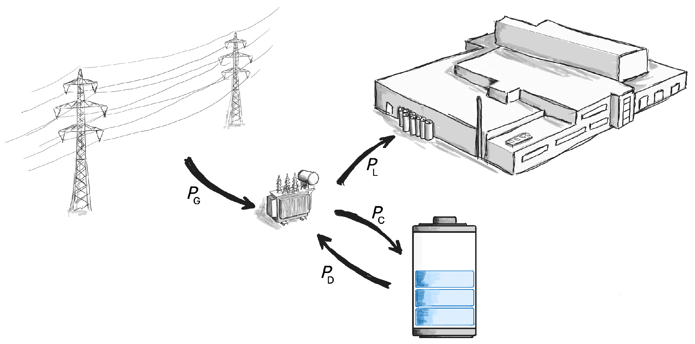
Figure 2.
Comparison of the real and the forecasted loads for one example day.
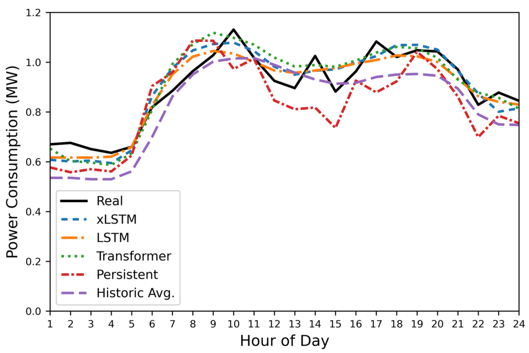
Figure 3.
Distribution of the daily forecasting errors in the test set of the different algorithms.
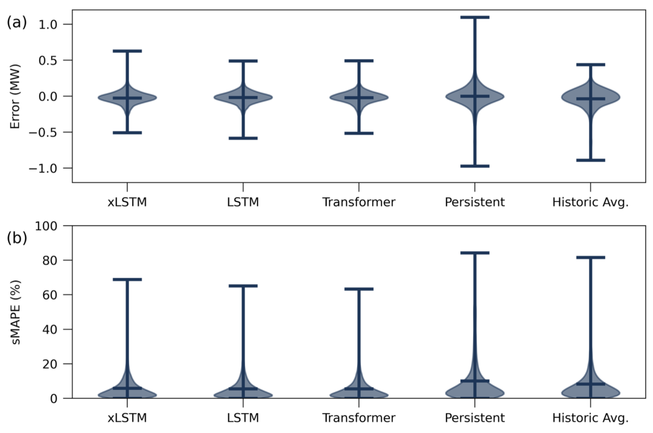
Figure 4.
Results of the simulation study comparing 2h, 4h and 6h BESS and different load forecasting algorithms. The algorithms are the columns in following order: perfect, xLSTM, LSTM, Transformer, persistent prediction and historical average load profile. The first row shows the revenue generated via load shifting. This does not include the investment and operation costs of the BESS, which are shown in the second row. The resulting yearly profit, assuming a lifetime of 15 years, is shown in row 3. Finally, the payback period and the ROI are shown, where the area without profit is shaded grey. The dotted vertical lines in column 3 are an example how to read the plot. The capacity leading to the highest profit for 4 h BESS is chosen. The other rows then show the DR revenue, BESS costs, payback period and ROI of this chosen BESS size.
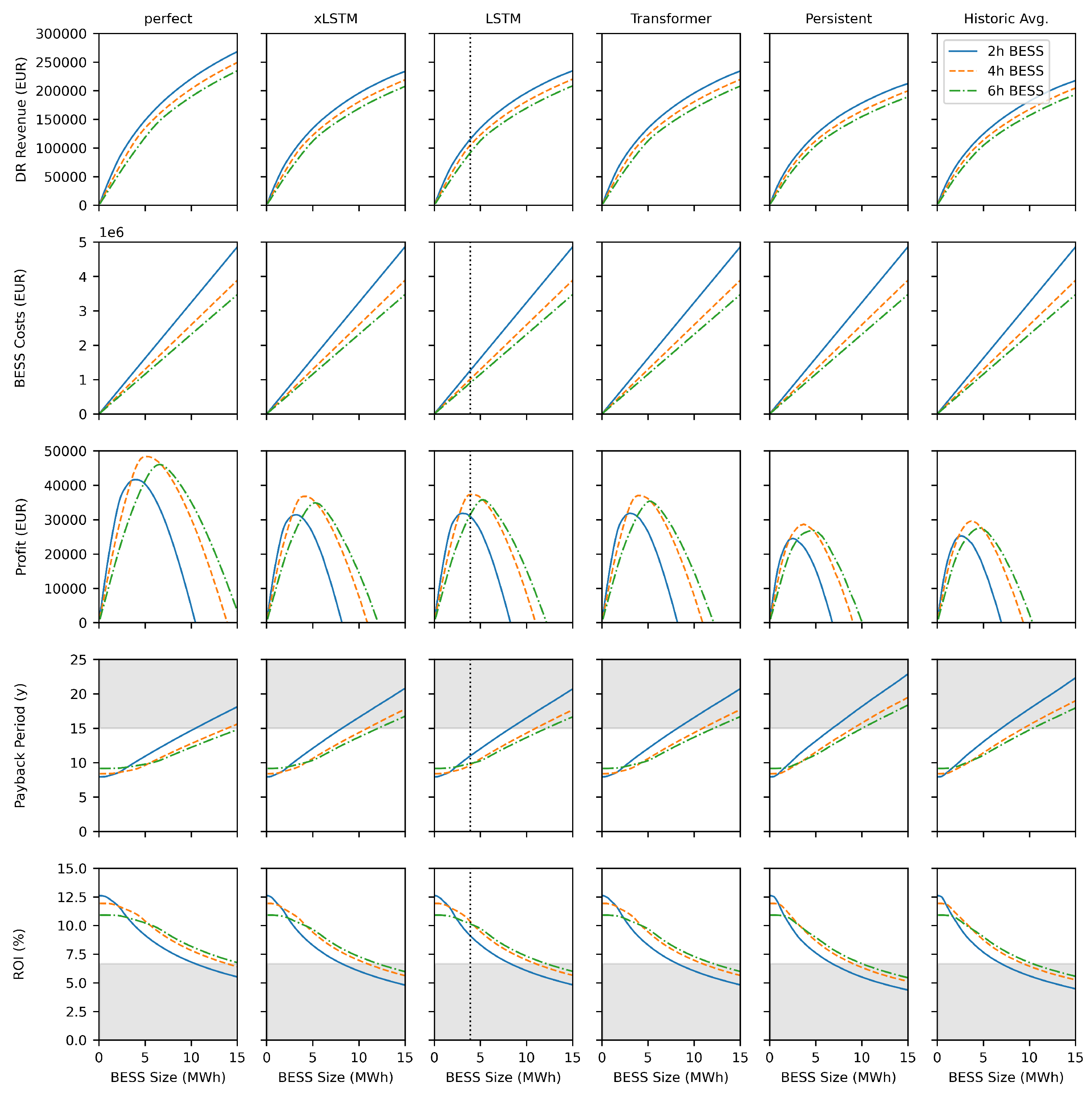
Figure 5.
Impact of different BESS price forecasts on the DR potential. The minimum, the average and the maximum price forecast of a 4h BESS are evaluated. a) shows the expected price development of a 4h BESS, b) shows the DR potential of the BESS for the predicted BESS costs, and c) shows the optimal BESS size.
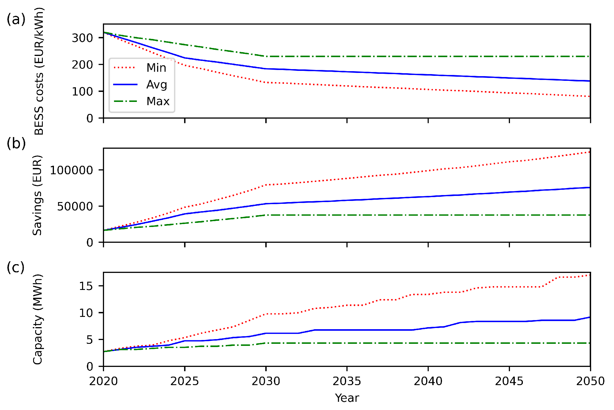

Table 1.
Configuration of the xLSTM, LSTM, and Transformer with approx. 10000 parameters.
| xLSTM | LSTM | Transformer | |
|---|---|---|---|
| Input | shape = (24 hours, 15 features) | ||
| Input Projection | yes | no | yes |
| Sequence Model | blocks = 2 heads = 4 features = 16 sLSTM at 1 |
layer 1 = 10 Bi-LSTM layer 2 = 18 Bi-LSTM |
layers = 1 heads = 4 feedforward dim = 10 features = 200 |
| Dense Layer 1 | 30 neurons, ReLU activation | ||
| Dense Layer 2 | 20 neurons, ReLU activation | ||
| Linear Layer | 1 neuron, no activation | ||
| Output | shape = (24 hours, 1 power value) | ||
Table 2.
Evaluation of the forecasting algorithms over the complete year.
| MAE (W) | sMAPE (%) | |
|---|---|---|
| Historical Avg. | 103944 | 16.59 |
| Persistent | 123978 | 20.08 |
| xLSTM | 69315 | 11.65 |
| LSTM | 65468 | 11.02 |
| Transformer | 65856 | 11.03 |
Table 3.
Case study results showing the profit for different BESS types and forecasting algorithms
| BESS type: | 2 h (EUR) | 4 h (EUR) | 6 h (EUR) |
|---|---|---|---|
| Perfect | 41,617 | 48,340 | 46,028 |
| Historical Avg. | 25,253 | 29,536 | 27,517 |
| Persistent | 24,465 | 28,585 | 26,800 |
| xLSTM | 31,380 | 36,738 | 34,836 |
| LSTM | 31,757 | 37,270 | 35,755 |
| Transformer | 31,762 | 36,981 | 35,370 |
Disclaimer/Publisher’s Note: The statements, opinions and data contained in all publications are solely those of the individual author(s) and contributor(s) and not of MDPI and/or the editor(s). MDPI and/or the editor(s) disclaim responsibility for any injury to people or property resulting from any ideas, methods, instructions or products referred to in the content. |
© 2025 by the authors. Licensee MDPI, Basel, Switzerland. This article is an open access article distributed under the terms and conditions of the Creative Commons Attribution (CC BY) license (http://creativecommons.org/licenses/by/4.0/).
Copyright: This open access article is published under a Creative Commons CC BY 4.0 license, which permit the free download, distribution, and reuse, provided that the author and preprint are cited in any reuse.


