A Mathematically Derived Unified Theoretical Framework Covering Special Relativity as a Special Case - “Asymmetry Theory"

Qian Chen

doi:10.20944/preprints202410.1330.v1

Submitted:

16 October 2024

Posted:

17 October 2024

You are already at the latest version

Abstract

We mathematically derived a comprehensive theoretic framework “Asymmetry Theory”, based solely on the well-established principle of “the constancy of the velocity of light” without any other assumptions, like the ether. This paper proves that Asymmetry Theory encompasses all results of Special Relativity (STR) as a special case when the observer moves perpendicularly to the “source-observer” line. It explains everything STR does but extends beyond it, offering novel and groundbreaking insights. The longstanding controversies surrounding STR arise from its application outside its intended special case, hence, they are all resolved in Asymmetry Theory. Asymmetry Theory is supported by all experiments supporting STR, like Kaufmann, Ives-Stilwell, muon lifetime, nuclear reaction…., and those contradicting STR, like the Lunar range and GPS tests of light speed and the lack of transverse Doppler shift. Despite its mathematical rigorousness and all experimental evidence, we propose two new experiments to decisively test predictions from both theories.The mathematically derived Asymmetry Theory is a more comprehensive theoretical framework covering STR as a special case. It is self-consistent and theoretically proved by Maxwell’s equations. It does not contradict any established physical observations but instead resolves century-old controversies by providing a unified, mathematical and paradox-free explanation of key phenomena. Furthermore, its groundbreaking results offer a unified perspective across various distinct laws of physics, including: A formula for light velocity mathematically explains the Sagnac effect, one-way light speed, stellar aberration, Michelson-Morley, Hafele-Keating and Optic clocks. Electrodynamics formulas encompass particle acceleration, Mass-Energy and matter wave. A unified formula for all cases of classical and transverse Doppler effects covers time-varying Doppler effect, cosmological redshift, and Cherenkov radiation. A generalized form of Maxwell's equations for moving observers directly derives the formulas for light speed, Doppler effect and Sagnac effect.

Keywords:

light speed

;

special relativity

;

Sagnac effect

;

Doppler effect

;

Maxwell’s Equations

;

time dilation

;

cosmological redshift

;

Cherenkov radiation

;

mass-energy

;

matter wave

;

particle acceleration

;

one-way light speed

;

abhorrence of starlight

;

Michelson-Morley

;

twin paradox

;

Lorentz transformation

;

asymmetry theory

;

Barnett experiment

;

Hafele-Keating

;

Ives-Stilwell

;

optical clocks

;

muon lifetime

;

Kaufmann-Bucherer-Neumann

;

nuclear reaction

;

lunar range test

Subject:

Physical Sciences - Theoretical Physics

I. Introduction

STR was mathematically derived based on two postulates (Einstein 1905 [1–3]). The second postulate stated: “in empty space, light is always propagated with a definite velocity V which is independent of the state of motion of the emitting body”. This principle of the constancy of the velocity of light, has been extensively validated by various experiments, including the uniformity of the timing signature of the binary x-ray pulsar system Her X1 [8], the speed of gamma rays emitted by fast pion [11], and the experiments with moving optical elements [12]. However, the further implicit assumption of STR that the light velocity is also independent of the motion of the observer has never been conclusively proven for 100 years. For example, Michelson-Morley-experiment [7] only proved that any variance in light speed was much smaller than Earth's orbital speed. Moreover, the Sagnac effect [15], observed in rotating frames, suggests an anomaly in the observer's perceived speed of light. Other experiments involving light speed measurements [26,27,39] also cast doubt on this assumption. Although many experiments appeared to support STR, those experiments contradicting it, like [14,27,39], were simply brushed away. There are also well-known paradoxes in STR, for example, the acceleration explanation of twin paradox conflicts with Hafele-Keating [29]. STR also claimed the one-way light speed as “un-measurable”. Other important theories of light velocity include the ether theory (Lorentz 1904 [6]) which relies on the existence of ether, and the emission theory (Ritz 1908 [9]) which contradicted the principle of constant light speed [10]. In summary, current theories have clear gaps in explaining key phenomena related to light.

The principle of the constancy of the velocity of light can be represented as

O (t_{o}) - S (t_{s}) = c (t_{o} - t_{s})

. Based solely on this equation without any other assumption, we mathematically derived a set of groundbreaking results, named “Asymmetry Theory” [23–25,35,40]. Not surprisingly, all STR results are shown mathematically as a special case of Asymmetry Theory (see Table 1).

In Section II, we mathematically derived a formula of light velocity, showing that while the light always propagates at constant speed c independent of the emitter’s motion, its velocity as detected by an observer is

c - v_{o} (t)

, where

v_{o} (t)

is the observer’s velocity relative to the light origin (Note: not the emitter). This asymmetry between the light “as propagated” vs. “as observed” should not be surprising. For example, the Doppler Effect [37] shows that different observers detect the same light at different frequencies depending on their motion. The Sagnac effect [15,16] is clear proof of this formula, which is simply due to the velocity difference of two light beams. This formula also mathematically explains one-way light velocity, Abhorrence of starlight, Michelson-Morley [7], Optical clocks [28], Hafele-Keating [29] and muon lifetime [31].

Section III discusses the “time scaling factor” to explain the phenomenon: when an observer moving away from a clock, the clock appears ticking slower and when the velocity approaches c, he will see the clock coming to a stall. If he compares the observed clock time with his clock time, he will see a “time scaling factor”, which is due to the asymmetry between the light emission time

t_{s}

at the light source and his observed time

t_{o}

, and mathematically represented as

d t_{o} / d t_{s}

. A formula of

d t_{o} / d t_{s}

is mathematically derived which resolves the “twin paradox”.

Section IV discusses the nature of Doppler effect [37], Cosmological redshift [21], and Cherenkov radiation [34], which is simply the “time-scaling factor”. A clock ticking slower/faster is equivalent to an “observed” lower/higher frequency. A unified formula is mathematically derived, which covers all traditional Doppler effect, Cosmological redshift, and Cherenkov radiation. Unlike current formulas, it also applies to time-varying velocities. This formula predicts no frequency shift for circular motion, supported by experiments [13,14]. By combining the effect of moving atomic clocks, a unified formula for all relativistic Doppler effects is mathematically derived, which mathematically explains the Ives-Stilwell experiments [30,36]. One unified formula covering so many traditionally different phenomena is self-telling.

Section V demonstrates the theoretical basis of Asymmetry Theory with Maxwell's equations. A generalized form of Maxwell’s equations for moving observer is mathematically transformed from the original equations [40]. From its solution, we mathematically derived the same results as Asymmetry Theory, including the formulas for light speed, Doppler effect and Sagnac effect. Again, no research ever achieved the results before. By revisiting Barnett’s experiment [18], we showed the Lorentz force is invariant under Galilean transformation. Correspondingly, the generalized Maxwell’s equations are shown to be covariant for different observer reference frames. Hence, the Lorentz transformation is not required in Asymmetry Theory.

Electrodynamics is discussed in Section VI. We mathematically derived a set of formulas, covering particle acceleration, mass-energy and matter wave, which explains why a particle is difficult to accelerate at high speed [32] and why the mass of a body emitting photons changes [33]. Our formula for particle acceleration also made a surprising prediction different from traditional belief like STR.

Section VII shows that all results of STR, including light speed equation, stellar aberration, time dilation, Doppler effect, particle acceleration and Mass-Energy can be mathematically represented as the special case of Asymmetry Theory when the observer is moving perpendicularly to the “source-observer” line. The difference is in the explanation of the same results. The longstanding controversies surrounding STR arise from its application outside this special case. Overcoming the limitations of STR, Asymmetry Theory provides mathematical and paradox-free explanations for key phenomena, even in rotating frame and with acceleration.

Any experiment supporting STR also supports Asymmetry Theory, for example, Optical clocks [28], Hafele-Keating [29], Ives-Stilwell [30,36], muon lifetime [31], Kaufmann [32] and nuclear reaction [33]. In addition, Asymmetry Theory is supported by those experiments contradicting STR, like the Lunar and GPS range test of light speed [27,39] and the lack of relativistic transverse Doppler shift [14].

While Asymmetry Theory is mathematically rigorous and supported by all existing experiments, we designed two experiments in Section VIII for further tests. One aims to measure Sagnac effect in inertia system and the second measures the momentum-to-acceleration ratios for high-speed particles with varying directions of applied momentum. By comparing the results with the predictions of both theories, a confirmative conclusion can be drawn.

II. The Velocity of Light

A. Notations

As in Figure 1, define

t_{s}

as the time when a light was emitted;

S (t_{s})

as the origin of the light emitted at

t_{s}

;

t_{o}

as the time an observer

O

observed the light from

S (t_{s})

;

O (t_{o})

as the position of

O

at

t_{o}

. Define

v_{o} (t_{o})

as the velocity of

O

relative to

S (t_{s})

at

t_{o}

and

v_{s} (t_{s})

denotes the velocity of the light source relative to

S (t_{s})

at

t_{s}

.

Note: The origin of the light

S (t_{s})

is different from the position of the emitter. They coincide at the emission

t_{s}

but are independent after

t_{s}

. Imagine an emitter sends a photon at

t_{s}

and immediately turns off. At

t_{s}

, the origin of light

S (t_{s})

is at the emitter’s position. After

t_{s},

the emitter’s motion won’t impact the previously emitted light i.e.

S (t_{s})

. An unrelated but helpful comparison is the position of a supersonic airplane vs. the origin of its sound wave.

B. Principle of Constant Light Velocity

Principle 1:

In empty space, the light always propagates with a velocity

c

. independent of the state of motion of the emitting body [1], which is mathematically represented with the general equation governing the velocity of light:

O (t_{o}) - S (t_{s}) = c (t_{o} - t_{s})

(1)

This paper is solely based on the mathematical derivation from equation (1) without any other assumption.

C. The Light Velocity/Speed Formula

First, let’s consider in the reference frame

F

in which

S (t_{s})

is static, where (1) becomes:

O (t_{o}) - S (t_{s}) = c (t_{o} - t_{s})

O (t_{s}) - S (t_{s}) + O (t_{o}) - O (t_{s}) = c (t_{o} - t_{s})

⟹ O (t_{s}) - S (t_{s}) + \int_{t_{s}}^{t_{o}} v_{o} (t) d t = c (t_{o} - t_{s})

⟹ O (t_{s}) - S (t_{s}) = \int_{t_{s}}^{t_{o}} (c - v_{o} (t)) d t

(2)

Then, for the same light origin

S (t_{s})

and observer

O

, (2) is proved covariant under the Galilean transformations from

F

to other reference frames (see App. A in [25]). Hence, (2) holds for any reference frame.

By definition, average speed = distance / travel time. We have:

Theorem 1

: The average speed for a light emitted from

S (t_{s})

to an observer

O

detecting it at

t_{o}

, is:

c_{s o} = |\int_{t_{s}}^{t_{o}} (c - v_{o} (t)) d t| / (t_{o} - t_{s})

(3)

Proof:

It is obvious from (2) and the definition.

∎

By definition, displacement = integral of velocity. Hence:

Lemma 1:

If a light is emitted from

S (t_{s})

to an observer

O

detecting it at

t_{o}

, the velocity of this light,

c_{so} (t)

, must satisfy, for any

t_{s}

and

t_{o}

,

O (t_{s}) - S (t_{s}) = \int_{t_{s}}^{t_{o}} c_{so} (t) d t

(4)

Theorem 2

: The velocity of a light emitted from

S (t_{s})

as to an observer

O

with velocity

v_{o} (t)

, is

c_{so} (t) = c - v_{o} (t)

(5)

Proof:

From (2) and (4) we have:

\int_{t_{s}}^{t_{o}} c_{so} (t) d t = \int_{t_{s}}^{t_{o}} (c - v_{o} (t)) d t

For this equation to hold for any

t_{s}

and

t_{o}

, we have:

c_{so} (t) = c - v_{o} (t) ∎

In summary,

Light velocity is independent of the emitter’s motion, i.e. $v_{s} (t)$ .
When $v_{o} (t) = 0$ , light velocity is constant $c$ .
The light velocity as to an observer depends on its velocity, specifically, $c - v_{o} (t)$ .

D. The One-Way Light Speed Measurement

The light velocity formula (5) is in harmony with the observation that one-way light speed can’t be measured at c. STR claimed it is impossible to measure one-way light speed due to clock synchronization error, which is not convincing since we should be able to control the error to a measurable range. (5) instead provides a straightforward explanation: one-way light velocity is not c, but

c - v_{o} (t)

.

E. Optical/Atomic Clock

Corollary 1:

The speed of light from

S (t_{s})

to

O (t_{o})

when

v_{o}

is perpendicular to

\vec{S (t_{s}) O (t_{s})}

is:

c_{s o} = c * \sqrt{1 - \frac{v_{o}^{2}}{c^{2}}}

(6)

This is a direct derivation from (5). It is important to note that the Lorentz factor is mathematically derived in (6).

An optical clock operates by measuring the frequency of photon vibrations. Since frequency is the inverse of cycle time, it is then proportional to the light speed. Let

f

be the frequency of a moving clock and

f = f_{0}

when

v_{o} = 0

, from (6) we have:

\frac{f}{f_{0}} = \frac{c_{s o}}{c} = \sqrt{1 - \frac{v_{o}^{2}}{c^{2}}}

(7)

In summary, the frequency of photon vibration decreases when an optical clock is moving, i.e. the clock slows down. It mathematically explains the Optical clocks [28], muon lifetime [31] and Hafele-Keating [29].

F. Round-Trip Light Speed & M-M Experiment

The formula (5) explains why the round-trip light speed is

c

and the null result for M-M experiment [7].

Corollary 2:

The round-trip speed of light from

S (t_{s})

to

O

with velocity

v_{o}

along the light path is:

c_{s o} = c * (1 - \frac{v_{o}^{2}}{c^{2}})

(8)

Proof

: From (5), we have

c_{s o} = \frac{2}{\frac{1}{c - v_{o}} + \frac{1}{c + v_{o}}} = c * (1 - \frac{v_{o}^{2}}{c^{2}}) ∎

In summary, the round-trip light speed

c_{s o} \approx c

if

v_{o} ≪ c

. If

v_{o} = 460 m / s

, the Earth orbital speed, the difference is only

0.7 mm / s

. Put it in the interferometer in Michelson-Morley [7], the difference is an undetectable 0.00005 fringe, which explains the null result.

G. Round-Trip Light Speed with Moving Reflector

The formula (5) explains the Lunar laser ranging test result of round-trip light speed (Gezari, 2009 [27]). In this test, the observatory moves along the line-of-sight of the reflector in moon at 200m/s due to the earth rotation, and the round-trip light speed is measured at

c

+200m/s.

Let the observatory velocities to the light origin and the reflector be

v_{o}

and

v_{r}

. So, the reflector velocity to the light origin is

v_{o} - v_{r} .

From (5), the round-trip speed

c_{s o}

is:

c_{s o} = \frac{2}{\frac{1}{c - {(v}_{o} - v_{r})} + \frac{1}{c + {(v}_{o} - v_{r})}} \approx c + v_{r}

In summary, while the Lunar laser ranging test of round-trip light speed appears to violate the invariance of

c

, it is a direct inference of the light velocity formula (5).

H. The Composition of Velocity

Assuming a light origin

S (t_{s})

, and two observers

O

and

O^{'}

with a relative velocity of

v

. The velocities of

O

and

O^{'}

relative to

S (t_{s})

,

v_{o^{'}} (t)

and

v_{o} (t)

follow:

v_{o^{'}} (t) - v_{o} (t) = v

Let

c_{so} (t)

and

c_{s o^{'}} (t)

be the velocity of the light from

S (t_{s})

to

O

and

O^{'}

. From (5), we have:

c_{s o^{'}} (t) = c - v_{o^{'}} (t) = c_{so} (t) - v

Hence, light velocity follows the addition of velocity.

I. The Sagnac Effect

The Sagnac effect [15] shows that two light beams, sent clockwise and counterclockwise around a closed path on a rotating disk, take different time intervals to travel the path, which contradicted the assumption that the light velocity is independent of the motion of the observer. STR attributed this contradiction to the rotating/accelerating frame [4,17]. The Sagnac effect can be extended to a FOG [16] with

Δ t = 2 v L / c^{2}

, where

v

is the speed of the detector,

L

is the length of the path.

Let

v_{o}^{+}

,

v_{o}^{-}

be the velocities of the detector to the origins of two light beams, then

v_{o}^{+} - v_{o}^{-} = 2 v

. According to (5), the light velocities as measured by the detector are

c - v_{o}^{+}

and

c - v_{o}^{-},

respectively. Therefore,

Δ t = \frac{L}{c - v_{o}^{+}} - \frac{L}{c - v_{o}^{-}} = \frac{2 v L}{(c - v_{o}^{-}) (c - v_{o}^{+})} \approx \frac{2 v L}{c^{2}}

In summary, the Sagnac effect is a direct inference of the light velocity formula (5) in Asymmetry Theory.

J. Key Angles and Stellar Aberration

Aberration of starlight is a phenomenon of difference in the observed angle of starlight due to the velocity of the observer. FIGURE 1 shows key angles for the velocity of light,

θ_{s}, θ_{o}, ϕ

. The stellar aberration is

θ_{o} - ϕ

. Assuming

v_{o} (t)

is constant

v_{o}

, the relationship is determined from Figure 1:

\sin (θ_{o} - ϕ) = \frac{v_{o}}{c} \sin (ϕ)

(9)

When

ϕ = 9 0^{°}

, from (9) we have

\cos (θ_{o}) = - v_{o} / c

. Hence,

θ_{o}

is the same as

ψ^{'}

in STR’s stellar aberration [1], and not a coincidence considering (6).

III. Time Scaling Factor

A. Time Scaling Factor

The time scaling factor is defined as

d t_{o} / d t_{s}

. From (1),

O (t_{o}) - S (t_{s}) = c (t_{o} - t_{s})

Perform an inner product of both sides, we have:

(O (t_{o}) - S (t_{s})) • (O (t_{o}) - S (t_{s})) = c^{2} {(t_{o} - t_{s})}^{2}

Differentiate both sides as to

t_{s}

and reorganize:

\frac{(O (t_{o}) - S (t_{s}))}{c (t_{o} - t_{s})} • (v_{o} (t_{o}) \frac{d t_{o}}{d t_{s}} - v_{s} (t_{s})) = c (\frac{d t_{o}}{d t_{s}} - 1)

Let

i_{o s}

denote the unit vector in

\vec{S (t_{s}) O (t_{s})}

, we have:

i_{o s} • v_{o} (t_{o}) \frac{d t_{o}}{d t_{s}} - i_{o s} • v_{s} (t_{s}) = c (\frac{d t_{o}}{d t_{s}} - 1)

Finally, the formula for time scaling factor is:

\frac{d t_{o}}{d t_{s}} = \frac{c - v_{s} (t_{s}) \cos (θ_{s})}{c + v_{o} (t_{o}) \cos (θ_{o})}

(10)

When

v_{o} (t), v_{s} (t)

are constant

v_{o}, v_{s}

and

θ_{s} = 0, θ_{o} = π

, (10) reduces to:

\frac{d t_{o}}{d t_{s}} = \frac{c - v_{s}}{c - v_{o}}

(11)

This formula (11) clearly explains the phenomenon of observed “time dilation” of a moving clock. When

v_{o}

increases, the observed elapsed time

d t_{o}

increases, i.e. the clock appears to tick slower. When

v_{o}

approaches

c

,

d t_{o}

approaches infinity, i.e. the clock appears to stall. Similarly, when

v_{o}

is negative,

d t_{o}

decreases, the clock appears to tick faster.

B. The “Twin Paradox”

Now consider the scenario of “twin paradox”. Assume a light source is at rest and an observer moves away from the same position and returns. Each records its time as

t_{s}

and

t_{o}

, with the start times synchronized as

t_{s} = t_{o} = 0

, and the return times as

t_{s} = t_{1}

and

t_{o} = t_{1} ’

, respectively.

The elapsed times recorded by each can be represented as

\int_{0}^{t_{1}} d t_{s}

and

\int_{0}^{t_{1}^{'}} d t_{o}

, respectively. Substituting

d t_{s}

with

d t_{o}

using (10), we have

\int_{0}^{t_{1}} d t_{s} = \int_{0}^{t_{1}^{'}} \frac{c + v_{o} (t_{o}) \cos (θ_{o})}{c} d t_{o}

= \int_{0}^{t_{1}^{'}} d t_{o} + \frac{1}{c} \int_{0}^{t_{1}^{'}} v_{o} (t_{o}) \cos (θ_{o}) d t_{o}

= \int_{0}^{t_{1}^{'}} d t_{o} + \frac{1}{c} \oint_{L} \cos (θ_{o}) d s

Where

d s

is the incremental distance over the path

L

. Since L is a closed contour,

\oint_{L} \cos (θ_{o}) d s = 0

. We have:

\int_{0}^{t_{1}} d t_{s} = \int_{0}^{t_{1}^{'}} d t_{o} o r t_{1} = t_{1}^{'}

which means the elapsed times measured by

t_{s}

and

t_{o}

are always the same independent of the movement. There is no “twin paradox” for the observed “time dilation” by time-scaling factor regardless of acceleration. Note: The impact of the optical/atomic clock is not considered in this case.

IV. The Doppler Effect

A. The General Formula for the Doppler Effect

The Doppler effect [37] is the change in frequency of a light to an observer who is moving relative to the light source. It is a straightforward mathematical derivation from the time scaling factor (10). Because the total wavenumber emitted during the period

d t_{s}

should be equal to that received during the period

d t_{o}

, we have:

f_{o} (t_{o}) * d t_{o} = f_{s} (t_{s}) * d t_{s}

Hence,

\frac{f_{s} (t_{s})}{f_{o} (t_{o})} = \frac{d t_{o}}{d t_{s}}

Applying (10), the general formula of Doppler effect is:

\frac{f_{s} (t_{s})}{f_{o} (t_{o})} = \frac{c - v_{s} (t_{s}) \cos (θ_{s})}{c + v_{o} (t_{o}) \cos (θ_{o})}

(12)

Assuming constant velocities

v_{o}, v_{s}

and

θ_{s} = 0, θ_{o} = π

, (12) reduce to the classical Doppler Effect formula [20]:

\frac{f_{s}}{f_{o}} = \frac{c - v_{s}}{c - v_{o}}

(13)

In summary, we mathematically derived the ground-breaking general formula (12) for classical Doppler effects with enhancement applicable to time-varying velocities.

B. The Doppler Effect of Atomic Clocks

The classical Doppler effect discussed in (12) does not consider the case when the emitter or observer is an atomic clock, which is demonstrated in the Ives–Stilwell experiments [30,36]. In this case, the frequency changes of atomic clocks themselves need to be included in the Doppler effect formula. Combine (7) and (12), we have:

\frac{f_{s} (t_{s}) \sqrt{1 - v_{s}^{2} (t_{s}) / c^{2}}}{f_{o} (t_{o}) \sqrt{1 - v_{o}^{2} (t_{o}) / c^{2}}} = \frac{c - v_{s} (t_{s}) c o s θ_{s}}{c + v_{o} (t_{o}) c o s θ_{o}}

The Doppler effect formula for atomic clocks is:

\frac{f_{s} (t_{s})}{f_{o} (t_{o})} = \frac{c - v_{s} (t_{s}) c o s θ_{s}}{c + v_{o} (t_{o}) c o s θ_{o}} * \frac{\sqrt{1 - v_{o}^{2} (t_{o}) / c^{2}}}{\sqrt{1 - v_{s}^{2} (t_{s}) / c^{2}}}

(14)

When

v_{o} (t_{o}) = 0 o r v_{s} (t_{s}) = 0

, (14) reduces to the well-known transverse Doppler effect formula supported by the Ives-Stilwell experiments [30,36]. In Sect. VII, we show that all current formulas of relativistic Doppler effect are just special cases of this general formula (14).

C. Experimental Support

Formula (12) explains the nature of Doppler effect as simply a phenomenon of time scaling factor. Since time scaling factor is a direct result of the varying propagation delay of light, Asymmetry theory predicts no frequency shift when the distance between the observer and the light source is constant. While STR [19] predicts a frequency shift for circular movement, experiment [14] agreed with Asymmetry Theory that there is no frequency shift.

In the case when the emitter or observer is an atomic clock, (14) in Asymmetry Theory is applied. When

v_{o} = 0, θ_{s} = 0,

(14) becomes:

\frac{f_{s}}{f_{o}} = \frac{\sqrt{1 - v_{s} / c}}{\sqrt{1 + v_{s} / c}}

which mathematically explains the results in the Ives-Stilwell type of experiments [30,36].

D. The Cosmological Red-Shift

Cosmological red-shift [21] is traditionally believed to be the effect of the inflating Universe and different from the Doppler Effect. Assume

a (t)

is the cosmic scale factor, the cosmological red-shift formula is:

\frac{f_{s} (t_{s})}{f_{o} (t_{o})} = \frac{a (t_{o})}{a (t_{s})}

(15)

In [24], we showed cosmological red-shift is a special case of the Doppler effect. Under the assumption of inflating Universe, equation (2) becomes:

O (t_{o}) - S (t_{s}) = \int_{t_{s}}^{t_{o}} c / a (t) d t

Following the similar mathematical derivation in III. A, we derived the corresponding formula:

\frac{f_{s} (t_{s})}{f_{o} (t_{o})} = \frac{c / a (t_{s}) - v_{s} (t_{s}) \cos (θ_{s})}{c / a (t_{o}) + v_{o} (t_{o}) \cos (θ_{o})}

(16)

When

v_{s} (t_{s}), v_{o} (t_{o}) ≪ c

\frac{f_{s} (t_{s})}{f_{o} (t_{o})} \approx \frac{a (t_{o})}{a (t_{s})}

which is the same as (15). Hence, the cosmological red-shift is a phenomenon of the time scaling factor

d t_{o} / d t_{s}

.

E. The Cherenkov Radiation

Cherenkov radiation [34] is electromagnetic radiation emitted when a charged particle passes through a dielectric medium at a speed greater than the light speed in that medium. It has conical wavefronts with a key emission angle

θ_{e}

determined by:

\cos (θ_{e}) = \frac{c}{n} / v_{p}

(17)

where

v_{p}

is the particle speed and

n

is the refractive index of the medium.

Let’s start derivation from (10). In this case, we have:

\frac{d t_{o}}{d t_{s}} = (\frac{c}{n} - v_{p} \cos (θ_{e})) / \frac{c}{n}

(18)

Now according to Fermat's principle, the light path should take the minimum time to the observer. We have:

\frac{d t_{o}}{d t_{s}} = 0

(19)

Substitute (19) to (18), we get the same formula as (17):

\cos (θ_{e}) = \frac{c}{n} / v_{p}

Hence, the Cherenkov radiation emission angle is mathematically derived from time scaling factor

d t_{o} / d t_{s}

.

V. Maxwell’s Equations

A. Maxwell Wave Equations to Observers

Maxwell’s standard wave equations [5] in a vacuum and charge-free space are:

\nabla^{2} E (r, t) - \frac{1}{c^{2}} \frac{\partial^{2}}{\partial t^{2}} E (r, t) = 0

(20)

\nabla^{2} B (r, t) - \frac{1}{c^{2}} \frac{\partial^{2}}{\partial t^{2}} B (r, t) = 0

(21)

Here,

t

is the time at light origin. In a reference frame that the emitter is static to the light origin,

t

is on the same scale as the time of the emitter, i.e.,

t_{s}

. (20) can be written as:

\nabla^{2} E (r, t_{s}) - \frac{1}{c^{2}} \frac{\partial^{2}}{\partial {t_{s}}^{2}} E (r, t_{s}) = 0

(22)

By solving (22), the light propagation velocity is constant

c

, consistent with Principle 1.

From the perspective of an observer, only the time it detects the light, i.e.

t_{o}

in Asymmetry Theory, can be used to measure the light propagation. Assume

v_{s} = 0

, and the observer has a velocity

v_{o}

along the direction of the light propagation. From (11), we have

\frac{d t_{o}}{d t_{s}} = \frac{c}{c - v_{o}}

(23)

Substitute

t_{s}

with

t_{o}

in (22), we have:

\nabla^{2} E (r, t_{o}) - \frac{1}{{(c - v_{o})}^{2}} \frac{\partial^{2}}{\partial {t_{o}}^{2}} E (r, t_{o}) = 0

(24)

Similarly,

\nabla^{2} B (r, t_{o}) - \frac{1}{{(c - v_{o})}^{2}} \frac{\partial^{2}}{\partial {t_{o}}^{2}} B (r, t_{o}) = 0

(25)

(24), (25) are the generalized Maxwell wave equations as to an observer. They are equivalent to the original Maxwell equations (20), (21), simply in another form using the time

t_{o}

from the perspectives of observer. When

v_{o} = 0

, they reduce to the original Maxwell equations.

B. Derivation of Light speed and Doppler Effect

The general solution to (24) is a linear superposition of waves of the form:

E (r, t_{o}) = g (2 π f_{o} t_{o} - k • r)

where

f_{o}

is the frequency observed by the observer,

k

is the wave vector and

k = |k|

is the wave number. From (24),

f_{o}, k

shall satisfy:

k^{2} - \frac{1}{{(c - v_{o})}^{2}} {(2 π f_{o})}^{2} = 0

Hence, the propagation speed

c_{s o}

is:

c_{s o} = \frac{2 π f_{o}}{k} = c - v_{o}

(26)

which is the same formula of light velocity derived in (5).

The observed frequency

f_{o}

is:

f_{o} = (c - v_{o}) * k / 2 π

Since the emission frequency is

f_{s} = c * k / 2 π

, we have:

\frac{f_{o}}{f_{s}} = \frac{c - v_{o}}{c}

which is the same formula as the Doppler effect in (13).

In summary, the formulas of light speed and Doppler effect in Asymmetry Theory can be mathematically derived from the solution of Maxwell equations, which provides the theoretical base and proof of the theory.

C. Generalized Maxwell Wave Equations

In [40], we further extend Maxwell’s equations to consider the general case when both the emitter and observer are moving. A general Maxwell’s equations for observers (27) were mathematically derived, which describes how the motions of emitter and observer impact the measurement.

({c^{2} \nabla}^{2} - (v_{s} ∙ \nabla) (v_{s} ∙ \nabla)) E (r, t_{o}) + 2 \frac{c - v_{s} \cos θ_{s}}{c + v_{o} \cos θ_{o}} (v_{s} ∙ \nabla) \frac{\partial}{\partial t_{o}} E (r, t_{o}) - \frac{{(c - v_{s} \cos θ_{s})}^{2}}{{(c + v_{o} \cos θ_{o})}^{2}} \frac{\partial^{2}}{\partial {t_{o}}^{2}} E (r, t_{o}) = 0

(27)

(27) reduces to the original Maxwell’s equations when

v_{s}

=

v_{o}

=0. In [40], we further show this general Maxwell’s equations (27) provide a unified solution consistent with experimental results in all scenarios of

v_{s},

v_{o}

. The formulas for light speed (5), Doppler effect (13) and Sagnac effect are all mathematically derived from solving (27), which again theoretically proves Asymmetry Theory.

D. Galilean Invariance of Lorentz Force

An electrical particle

P

with charge

q

in an electrical and magnetic field will experience the Lorentz force [22] of

f = q * (E + v \times B)

(28)

Traditionally,

v

is defined as the velocity of

P

in any chosen reference frame. In Barnett’s experiment [18], a cylindrical capacitor with a fine wire shorting its inner and outer conductors is coaxial with a solenoid magnet. In case 1, the capacitor rotates with angular velocity

ω

, while the solenoid is at rest. Lorentz force is detected. In case 2, the capacitor is at rest, but the solenoid rotates with

ω

. No Lorentz force is detected. This result clearly showed that only the motion relative to the magnetic field generates Lorentz force and invalidated the traditional belief.

Like the light origin, let

S

be the center of the magnetic field

B

. Define

v

as the velocity of

P

relative to

S

:

v = \frac{d (P - S)}{d t}

Since the center

S

is in the axis, in case 1,

v = ω * r

, while in case 2,

v = 0 .

Barnett’s experiment is explained.

If we perform the Galilean transformation,

P, S, E, B

become

P^{'}, S^{'}, E^{'}, B^{'}

after transformation. We should have the same Lorentz force after transformation. Hence,

q * (E^{'} + v^{'} \times B^{'}) = q * (E + v \times B)

(29)

Since

v^{'} = \frac{d (P^{'} - S^{'})}{d t^{'}} = \frac{d (P - S)}{d t} = v

for (29) to hold for any

v

, we have:

E^{'} = E and B^{'} = B

(30)

In summary, The Lorentz force law is invariant under Galilean transformation and the fields don’t change simply due to transformation of coordinates.

E. The Covariance of Maxwell’s Equations

For simplicity, assume the light is polarized moving in the x-direction. The Maxwell equations (24) for an observer

O

in frame

F

becomes:

\frac{\partial^{2}}{\partial x^{2}} E - \frac{1}{{(c - v_{o})}^{2}} \frac{\partial^{2}}{\partial {t_{o}}^{2}} E = 0

(31)

Perform the Galilean transformation from

F

to a new observer frame

F^{'}

. Let

v_{o}, t_{o}, t, E

become

v_{o}^{'}, t_{o}^{'}, t^{'}, E^{'}

after transformation. From (23) we have

\frac{d t_{o} ’}{d t^{'}} = \frac{c}{c - v_{o} ’} a n d \frac{d t_{o}}{d t} = \frac{c}{c - v_{o}}

Since

t^{'} = t

, we have

\frac{d t_{o}}{c - v_{o}} = \frac{d t_{o}'}{c - v_{o}'}

Since

E^{'} = E

from (30), substituting

t_{o}, v_{o}

with

t_{o}^{'}, v_{o} ’

in (31), we have:

\frac{\partial^{2}}{\partial x'^{2}} E^{'} - \frac{1}{{(c - v_{o}')}^{2}} \frac{\partial^{2}}{\partial t_{o}'^{2}} E^{'} = 0

In summary, the generalized form of Maxwell equations is covariant for different reference frames and Lorentz transformation is not required in Asymmetry Theory.

VI. Electrodynamics

Like STR [1,2], a set of electrodynamics formulas is mathematically derived from the light velocity formula (5).

A. Momentum to Acceleration Ratio

It is well known that a particle becomes difficult to accelerate when its speed approaches

c

[32], which can be simply explained as the electromagnetic wave’s speed relative to the particle according to (5).

Assuming a particle has a mass

m

and a velocity

v_{o}

, and it gained an incremental velocity

Δ v_{o}

with the applied momentum

Δ P

from the photons. According to (5), the velocity of the photons relative to the particle is

c - v_{o}

. The equation of momentum conservation for the case of perfectly inelastic collision is:

\frac{Δ P}{c} |c - v_{o}| = m * Δ v_{o}

(32)

When

c

and

v_{o}

are in the same direction, (32) becomes:

\frac{Δ P}{Δ v_{o}} = m / (1 - \frac{v_{o}}{c})

(33)

When

v_{o}

increases, the momentum to acceleration ratio increases. When

v_{o}

approaches

c

, the ratio approaches infinity, i.e. the particle can no longer be accelerated.

The key prediction from (32) is that the momentum to acceleration ratio depends on both the velocity and the direction of momentum. Assume

v_{o} = c / 2

and then the direction is reversed, i.e.

v_{o} = - c / 2

, a 3x ratio change is predicted. This surprising prediction, different from STR [1], is utilized to validate Asymmetry Theory in VIII.

B. The Mass-Energy Relationship

If photons are absorbed by a particle and let

Δ m

denotes the incremental mass after the absorption, we have the following equation for momentum conservation:

Δ P + m v_{o} = (m + Δ m) * (v_{o} + Δ v_{o})

\Rightarrow Δ P + m v_{o} = m v_{o} + Δ m v_{o} + m Δ v_{o} + Δ m Δ v_{o}

Omit the second order

Δ m Δ v_{o}

and substitute

m Δ v_{o}

with (33), we have:

Δ P = Δ m v_{o} + Δ P / c * (c - v_{o})

(34)

\Rightarrow Δ P * c = Δ m * c^{2}

Hence, we derived the Mass-Energy relationship:

Δ E = Δ m * c^{2}

(35)

This Mass-Energy relationship (35) is in harmony with STR [2] and explains the relationship between mass change and released energy [33].

C. Mass Change and Matter Wave

Substitute

Δ P

in (34) with (32), we have:

m * Δ v_{o} * \frac{v_{o}}{c - v_{o}} = Δ m * v_{o}

\Rightarrow \frac{d m}{m} = d (\frac{v_{o}}{c}) / (1 - \frac{v_{o}}{c})

Integrate from

v_{o} = 0 t o v

, the mass change formula is:

m (v) = m (0) / (1 - \frac{v}{c})

(36)

Applying De Broglie matter wave formula [41],

m (v) * v = h / λ

where

λ

is the wavelength, (36) becomes:

(m (v) - m (0)) * c = h / λ

Applying (35), the energy and matter wave relationship is:

Δ E = h * c / λ

(37)

VII. STR as a Special Case

All results of STR can be mathematically represented as a special case of Asymmetry Theory when the observer is moving perpendicularly to the “source-observer” line, i.e.

ϕ = 9 0^{°}

in Figure 1.

A. Distance and Light Speed

When

ϕ = 9 0^{°}

, Asymmetry Theory (6) and STR [1] provides the same equation governing distance d and c:

d = c * \sqrt{1 - \frac{v_{o}^{2}}{c^{2}}} * t

(38)

The only difference is how to explain (38). STR is forced to assume a varying time

t

to make (38) hold. Asymmetry Theory derives the light speed from (38) as:

c_{s o} = c * \sqrt{1 - \frac{v_{o}^{2}}{c^{2}}}

Hence, (38) always holds in Asymmetry Theory and there is no need to change time

t

.

B. Stellar Aberration

When

ϕ = 9 0^{°}

, the formula (9) of stellar aberration in Asymmetry Theory becomes:

\cos (θ_{o}) = - v_{o} / c

(39)

which is the same as in STR [1], noting

ψ^{'} = θ_{o}

.

C. Time Dilation/Optical Clock

When

ϕ = 9 0^{°}

, let

f

be the optical clock frequency and let it be

f_{0}

when

v_{o} = 0

, from (6) we have:

\frac{f}{f_{0}} = \frac{c_{s o}}{c} = \sqrt{1 - \frac{v_{o}^{2}}{c^{2}}}

(40)

This is the same as the time dilation formula in STR [1]. Again, the only difference is STR explains the variation of clock frequency

f

in (40) as the variation of time

t

.

(40) is in harmony with the optical clocks [27], Hafele-Keating [28] and muon lifetime [31]. The Hafele-Keating results prove that each clock depends on its own specific velocity, i.e.

v_{o}

in (40), and the twin with the lowest

v_{o}

has the slowest clock. It supports Asymmetry Theory but contradicts STR’s explanation that the twin with no acceleration experiences the minimum time.

D. Relativistic Doppler Effect

Currently, different formulas are required for STR’s relativistic Doppler effect in different scenarios [19]. All these formulas are just special cases of our Doppler effect formula for atomic clocks (14). Assuming constant velocity, (14) reduces to:

\frac{f_{s}}{f_{o}} = \frac{c - v_{s} c o s θ_{s}}{c + v_{o} c o s θ_{o}} * \frac{\sqrt{1 - v_{o}^{2} / c^{2}}}{\sqrt{1 - v_{s}^{2} / c^{2}}}

(41)

The following table shows how (41) reduces to the relativistic Doppler effect in different scenarios. The fact that one unified formula covers all scenarios is self-telling.

Scenario	Case	$f_{s} / f_{o}$
Relativistic longitudinal	$v_{s} = 0,$ $θ_{o} = π$	$\sqrt{1 + v_{o} / c} / \sqrt{1 - v_{o} / c}$
Transverse visual closest	$v_{s} = 0,$ $θ_{o} = π / 2$	$\sqrt{1 - {v_{o}}^{2} / c^{2}}$
Transverse geometric closest	$v_{o} = 0,$ $θ_{s} = π / 2$	1/ $\sqrt{1 - {v_{s}}^{2} / c^{2}}$
Receiver circular motion	$v_{s} = 0,$ $θ_{o} = π / 2$	$\sqrt{1 - {v_{o}}^{2} / c^{2}}$
Source circular motion	$v_{o} = 0,$ $θ_{s} = π / 2$	1/ $\sqrt{1 - {v_{s}}^{2} / c^{2}}$
Source & receiver circular motion	$θ_{o} = π / 2$ $θ_{s} = π / 2$	$\sqrt{(c^{2} {- v}_{o}^{2}) / (c^{2} {- v}_{s}^{2})}$
Receiver motion arbitrary direction	$v_{s} = 0$	$\sqrt{1 - {v_{o}}^{2} / c^{2}} / (1 + v_{o} / c * \cos θ_{o})$
Source motion arbitrary direction	$v_{o} = 0$	$(1 - v_{s} / c * \cos θ_{s})$ $/ \sqrt{1 - {v_{s}}^{2} / c^{2}}$

E. Particle Acceleration

When

ϕ = 9 0^{°}

, the momentum formula (32)

\frac{Δ P}{c} |c - v_{o}| = m * Δ v_{o}

becomes:

\frac{Δ P}{Δ v_{o}} = m / \sqrt{(1 - \frac{{v_{o}}^{2}}{c^{2}})}

(42)

This is the same formula in STR [1] and is supported by Kaufmann experiment [32].

The longstanding controversies around STR arose when people tried to apply it outside the special case. For example, (42) is valid only when

ϕ = 9 0^{°}

. But when STR tries to apply (42) to all cases, it implies the momentum formula is directionless. The broader formula (32) of Asymmetry Theory predicts the momentum ratio depends on the direction of momentum, i.e. it is harder to accelerate a particle at high speed, but easier to decelerate it. An experiment is designed in VIII. to test which theory is right.

F. Mass Energy Relationship

The formula of mass energy relations (35) is mathematically derived in Asymmetry Theory as

Δ E = Δ m * c^{2}

The well-known formula (43) in STR [1] is just a special case of (35). In fact, if (43) is true, (35) must be true.

E = m * c^{2}

(43)

The experiment of nuclear reaction [33] is aligned more directly with formula (35) than (43), i.e. released energy is related to the mass change, i.e.

Δ m

in (35).

G. Experimental Support

Any experiment that supports STR also supports Asymmetry Theory. In addition, Asymmetry Theory is in harmony with experiments [14,27,39] contradicting STR:

1. Doppler effect in circular motion. STR predicts transverse Doppler effect for any circular motion. In Asymmetry Theory, transverse Doppler effect (14) only applies to atomic clocks. In other cases, since

θ_{o} = 90^{o}

for circular motion, formula (12) becomes:

f_{s} (t_{s}) / f_{o} (t_{o}) = 1

which means no Doppler effect. The experiment [14] confirms the lack of relativistic transverse Doppler shift for microwave device in circular motion.

2. One-way light speed. Since one-way light speed was never measured to be

c

, STR claimed that it can’t be measured at all. Asymmetry Theory provides a straightforward formula (5) for one-way light velocity

c - v_{o} (t)

, which is supported by the GPS test of light speed [39]. In this test, the light speed measured by GPS is

c \pm v

depending on the direction to satellite, where

v

is the rotation velocity of the Earth.

3. Round trip light speed with moving reflector. When there is a relative speed

v_{r}

between the observer and the reflector, STR predicts the round-trip light speed to be invariant

c

. Asymmetry Theory calculates the light speed to be

c + v_{r}

, which is in harmony with the lunar laser ranging test of round-trip light speed [27]. In this test, the observatory moves along the line-of-sight of the reflector in moon at 200m/s due to the earth rotation, and the light speed is measured at

c + 200 m / s

.

VIII. Experiments Design

Two experiments are designed in [23] to test different predictions of Asymmetry Theory and STR.

A. Light Velocity to Moving Observers

First experiment [23] originated from the Sagnac effect. STR tried to brush away the anomaly of Sagnac effect with the rotating frame. Hence, we try to test it in an inertial system. A transient light source and two moving light sensors are in the same initial position and connected to the same precise digital scope, see Figure 2. This setup is to avoid the synchronization argument by STR. A high-speed camera is an optional enhancement to capture the exact moments when the photon hits the sensors. Both sensors are moving at a constant speed

v

but in opposite directions. Light is emitted when both sensors are in the same position. The detection times of reflected light are measured.

If the light velocity is independent of the motion of observers, both sensors shall detect the light at the same moment. Instead, Asymmetry Theory predicts a difference

Δ t = 2 v L / (c^{2} - v^{2})

, same as the Sagnac effect. As long as there is a measurable time difference or a sequence of detections captured by the camera, it will invalidate the assumption of light-speed invariance to moving observers.

B. Asymmetry of Momentum to Acceleration

The second experiment [23] is based on the prediction of asymmetry of acceleration/deceleration of particles (32) in Asymmetry Theory, see Figure 3. Let a particle run at a constant high speed, say

0.5 c

. Then apply a momentum and measure the ratio of the applied momentum to the speed change. Finally, repeat the same experiment with same momentum, but change the direction of applied momentum every time.

According to the relativistic mass/energy (42) in STR, the momentum to speed change ratio is directionless, i.e. the ratio should remain constant despite the change of direction. However, according to the formula (32) of Asymmetry theory, the momentum to speed change ratios will be dramatically different between the directions of acceleration and deceleration, say 3X. The result should confirm which prediction is correct.

IX. Conclusions

In summary, Asymmetry Theory is mathematically derived based solely on the well-established principle of constant light velocity without any other assumption, like the existence of ether.

STR is mathematically represented as a special case of Asymmetry Theory. Any e xperiment supporting STR also supports Asymmetry Theory. Asymmetry Theory is also in harmony with the experiments contradicting STR and provides unified and mathematical explanations of key phenomena without any paradox. A summary of comparison with STR and the supporting experiments is presented in Table 1.

Asymmetry Theory is comprehensive, self-consistent, and in harmony with all existing experiments. Maxell’s equations provide further theoretical proof. Its groundbreaking results unified key physical theories in different domains, including a unified formula of Doppler effect and the generalized Maxwell’s equations. Two experiments are designed to test different predictions of both theories, which should confirm which is correct.

Data Statements

The data that supports the findings of this study are available within the article.

Acknowledgements

This research is sponsored by The International Education Foundation.

References

Einstein, On the Electrodynamics of Moving Bodies, Annalen der Physik, 17, 891-921 (1905).
Einstein, Does the Inertia of a Body Depend Upon its Energy-Content?, Annalen der Physik, 323 (13): 639–641 (1905).
Einstein, On the Possibility of a New Test of the Relativity Principle, Annalen der Physik, 328 (6): 197–198 (1907).
Einstein, Generalized theory of relativity, the anthology ‘The Principle of Relativity’, 94, University of Calcutta (1920).
J. Maxwell, A Dynamical Theory of the Electromagnetic Field, Philos. Trans. R. Soc. Lond. 155, 459-512 (1865).
H. Lorentz, Electromagnetic phenomena in a system moving with any velocity smaller than that of light, Proc. R. Neth. Acad. Arts Sci. 6: 809–831 (1904).
Michelson and, E. Morley, On the Relative Motion of the Earth and the Luminiferous Ether, Am. J. Sci. 34 (203): 333–345 (1887).
K. Brecher, Phys. Rev. Lett., 39, 1051 (1977).
W. Ritz, Recherches Critiques sur les Theories Electrodynamiques de Cl. Maxwell et de H.-A. Lorentz, Archives des Sciences physiques et naturelles 36: 209 (1908).
J. G. Fox, Evidence Against Emission Theories, Am. J. Phys. 33, 1–17 (1965).
F. Alvaeger et al., Phys. Lett. 12, 260 (1964).
G. C. Babcock et al., J. O. S. A. 54, 147 (1964).
D.C. Champeney et al., Absence of Doppler shift for gamma ray source and detector on same circular orbit., Proc. Phys. Soc. 77, 350 (1961).
H. W. THIM, Absence of the relativistic transverse Doppler shift at microwave frequencies, IEEE Trans. Instr. Measur. 52, 1660-1664 (2003).
G. Sagnac, C. R. Acad. Sci. Paris 157, 708 (1913).
R. Wang et al., Physics Letters A. 312 (1–2): 7–10 (2006).
Langevin, Paul, Sur la théorie de la relativité et l'expérience de M. Sagnac, Comptes Rendus. 173: 831–834 (1921).
S.J. Barnett, On Electromagnetic Induction and Relative Motion, Phys. Rev. 35, 323 (1912).
D. Sher, The Relativistic Doppler Effect, J. R. Astron. Soc. Can. 62: 105–111 (1968).
N. Giordano, College Physics: Reasoning and Relationships, Cengage Learning, 421–424 (2009).
T. Koupelis et al., In Quest of the Universe, Jones & Bartlett Publishers, 557 (2007).
H. Lorentz, Versuch einer Theorie der electrischen und optischen Erscheinungen in bewegten Körpern, Leiden: E.J. Brill (1895).
Q. Chen, Design of Experiments for Light Speed Invariance to Moving Observers, submitted to Int. J. Theor. Phys. [CrossRef]
Q. Chen, Time-varying Doppler Effect formula and its application in Cosmology. [CrossRef]
Q. Chen, Asymmetry Theory mathematically derived from the principle of constant light speed. [CrossRef]
Nelson, R.A. et al., Experimental Comparison of Time Synchronization Techniques by Means of Light Signals and Clock Transport on the Rotating Earth, Proc. 24th Annual PTTI Systems and Applications Meeting: 87-104, (1993).
Gezari, D.Y., Lunar laser ranging test of the invariance of c, arXiv 0912.3934 (2009).
Chou, C. et al., Optical clocks and Relativity, Science. 329, 1630-1633 (2010).
Hafele, J. C.; et al. Around-the-World Atomic Clocks: Observed Relativistic Time Gains, Science. 177, 168-170 (1972).
Ives, H. E.; et al. An experimental study of the rate of a moving atomic clock, J. O. S. A. 28, 215 (1938).
Rossi, B.; et al. Variation of the Rate of Decay of Mesotrons with Momentum, Physical Review. 59, 223–228 (1941).
Kaufmann, W. Die magnetische und elektrische Ablenkbarkeit der Bequerelstrahlen und die scheinbare Masse der Elektronen, Göttinger Nachrichten (2): 143–168 (1901).
Oliphant, M. L. E.; et al. "The Transformation of Lithium by Protons and by Ions of the Heavy Isotope of Hydrogen". Proc. R. Soc. 141, 722–733 (1933).
Cherenkov, P. A. Visible emission of clean liquids by action of γ radiation, Doklady Akademii Nauk SSSR. 2: 451 (1934).
Q. Chen, A mathematically-derived unified formula for Time-Varying Doppler effect, Cosmological red-shift and Cherenkov radiation, Optica Open doi.org/10.1364/opticaopen.25612566.v1 (2024).
S. Reinhardt et al., Test of relativistic time dilation with fast optical atomic clocks at different velocities, Nature Physics. 3, 861–864 (2007).
Doppler, Beiträge zur fixsternenkunde, Prague: G. Haase Söhne, 69 (1846).
Bélopolsky, On an Apparatus for the Laboratory Demonstration of the Doppler-Fizeau Principle, ApJ. 13, 15 (1901).
P. Marmet, The GPS and the Constant Velocity of Light, Acta Scientiarum, 22, 1269 (2000).
Q. Chen, Revisiting Maxwell's Equations for Observers, Preprints. doi.org/10.20944/preprints202408.0897.v1 (2024).
L. de Broglie, “Recherches sur la théorie des quanta”, Thèse de doctorat soutenue à Paris (1924).

Figure 1. Timing, Velocities and Key angles.

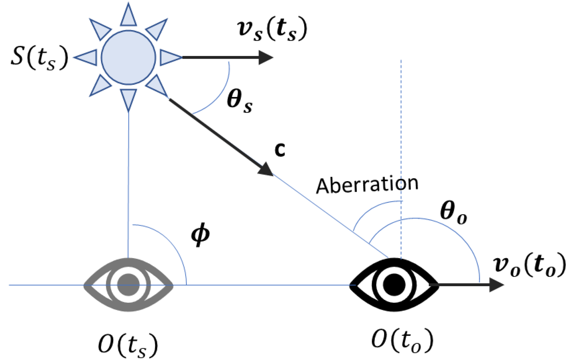
Figure 2. Setup for light speed to moving observers [2][].

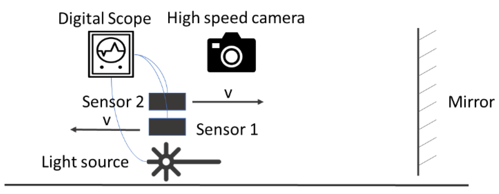
Figure 3. Ratios of momentum to speed change [23].

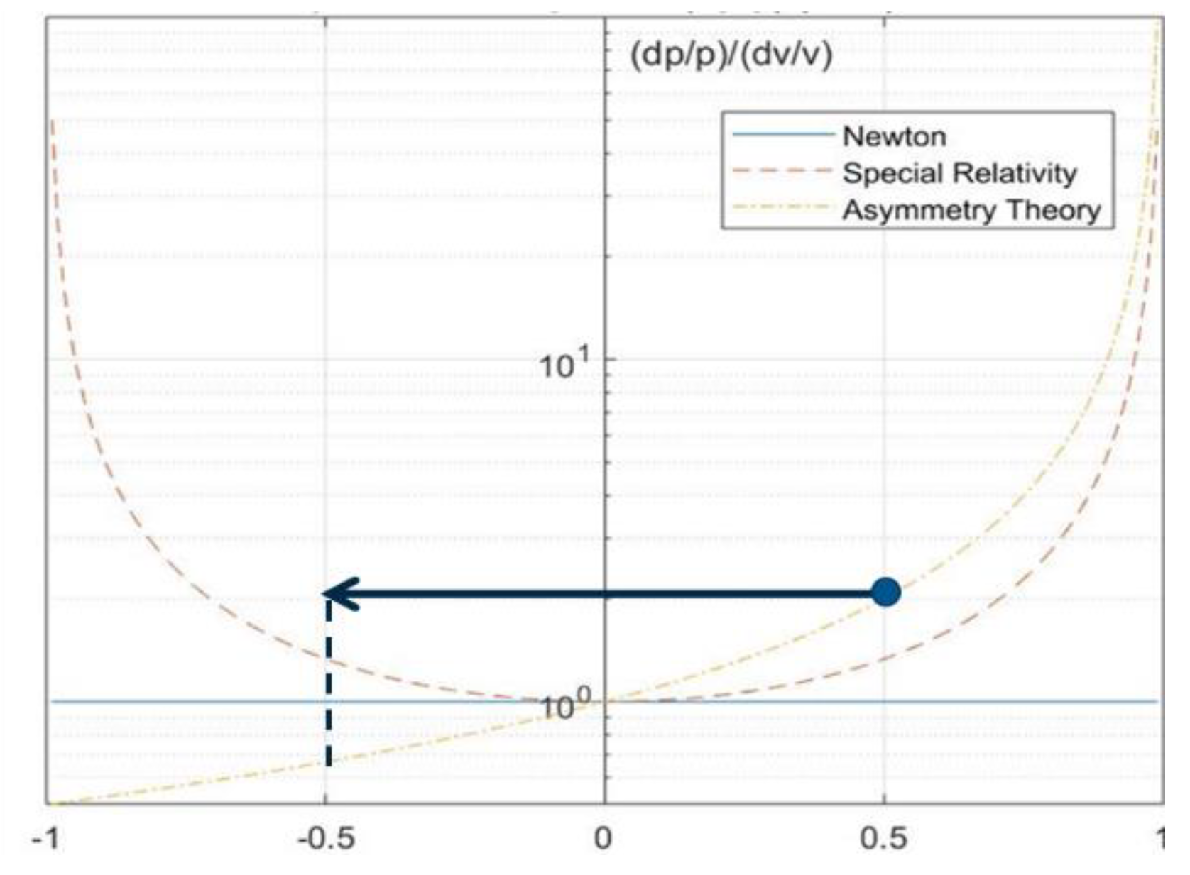
Table 1. Comparison of Asymmetry Theory and Special relativity including experiments.

	Asymmetry Theory	Special Relativity	Supporting Experiments*^#
Distance and light speed equation	$d = c * \sqrt{1 - v_{o}^{2} / c^{2}} * t$	$d = c * \sqrt{1 - v^{2} / c^{2}} * t$
Optical clock	$\frac{f}{f_{0}} = \frac{c_{s o}}{c} = \sqrt{1 - v_{o}^{2} / c^{2}}$	$\frac{t}{t_{0}} = \sqrt{1 - v^{2} / c^{2}}$	muon life [31]; Optical clock [28]; Hafele-Keating [29]
One-way light speed	$c_{s o} = \|c - v_{o}\|$	Not measurable	GPS test of light speed* [39]
Two-way light speed	$c_{s o} = c * (1 - v_{o}^{2} / c^{2}) \approx c$	$c$	Michelson-Morley [7]
Two-way light speed with motion	$c_{s o} \approx c + v_{r}$	$c$	Lunar range test of light speed* [27]
Stellar Aberration	$\cos (θ_{o}) = - v_{o} / c$	$\cos (ψ^{'}) = - v / c$	Stellar aberration
Sagnac effect	$Δ t = \frac{2 v L}{(c - v_{o}^{-}) (c - v_{o}^{+})}$	Not applicable	Sagnac effect^# [15,16]
Doppler effect	$\frac{f_{s} (t_{s})}{f_{o} (t_{o})} = \frac{c - v_{s} (t_{s}) c o s θ_{s}}{c + v_{o} (t_{o}) c o s θ_{o}}$	$\frac{f_{s}}{f_{o}} = \frac{\sqrt{1 + v / c}}{\sqrt{1 - v / c}}$	Lack of relativistic Doppler effect* [14]; Cosmological redshift^# [21]
Doppler effect for Atomic clock	$\frac{f_{s}}{f_{o}} = \frac{c - v_{s} c o s θ_{s}}{c + v_{o} c o s θ_{o}} * \frac{\sqrt{1 - v_{o}^{2} / c^{2}}}{\sqrt{1 - v_{s}^{2} / c^{2}}}$	$\frac{f_{s}}{f_{o}} = \frac{\sqrt{1 + v / c}}{\sqrt{1 - v / c}}$	Ives-Stilwell [30,36]
Particle Momentum	$\frac{Δ P}{Δ v_{o}} = m * c / \|c - v_{o}\|$	$\frac{Δ P}{Δ v} = m / \sqrt{1 - v^{2} / c^{2}}$	Kaufmann [32]
Mass-energy relationship	$Δ E = Δ m * c^{2}$	$E = m * c^{2}$	Nuclear reaction [33]

Note: * Support Asymmetry Theory but contradict Special Relativity; ^# Not applicable to Special Relativity.

Disclaimer/Publisher’s Note: The statements, opinions and data contained in all publications are solely those of the individual author(s) and contributor(s) and not of MDPI and/or the editor(s). MDPI and/or the editor(s) disclaim responsibility for any injury to people or property resulting from any ideas, methods, instructions or products referred to in the content.

© 2024 by the authors. Licensee MDPI, Basel, Switzerland. This article is an open access article distributed under the terms and conditions of the Creative Commons Attribution (CC BY) license (http://creativecommons.org/licenses/by/4.0/).

Copyright: This open access article is published under a Creative Commons CC BY 4.0 license, which permit the free download, distribution, and reuse, provided that the author and preprint are cited in any reuse.

A Mathematically Derived Unified Theoretical Framework Covering Special Relativity as a Special Case - “Asymmetry Theory"

Abstract

Keywords:

Subject:

I. Introduction

II. The Velocity of Light

A. Notations

B. Principle of Constant Light Velocity

C. The Light Velocity/Speed Formula

D. The One-Way Light Speed Measurement

E. Optical/Atomic Clock

F. Round-Trip Light Speed & M-M Experiment

G. Round-Trip Light Speed with Moving Reflector

H. The Composition of Velocity

I. The Sagnac Effect

J. Key Angles and Stellar Aberration

III. Time Scaling Factor

A. Time Scaling Factor

B. The “Twin Paradox”

IV. The Doppler Effect

A. The General Formula for the Doppler Effect

B. The Doppler Effect of Atomic Clocks

C. Experimental Support

D. The Cosmological Red-Shift

E. The Cherenkov Radiation

V. Maxwell’s Equations

A. Maxwell Wave Equations to Observers

B. Derivation of Light speed and Doppler Effect

C. Generalized Maxwell Wave Equations

D. Galilean Invariance of Lorentz Force

E. The Covariance of Maxwell’s Equations

VI. Electrodynamics

A. Momentum to Acceleration Ratio

B. The Mass-Energy Relationship

C. Mass Change and Matter Wave

VII. STR as a Special Case

A. Distance and Light Speed

B. Stellar Aberration

C. Time Dilation/Optical Clock

D. Relativistic Doppler Effect

E. Particle Acceleration

F. Mass Energy Relationship

G. Experimental Support

VIII. Experiments Design

A. Light Velocity to Moving Observers

B. Asymmetry of Momentum to Acceleration

IX. Conclusions

Data Statements

Acknowledgements

References

MDPI Initiatives

Important Links

Subscribe