Submitted:
12 October 2024
Posted:
14 October 2024
You are already at the latest version
Abstract
Seafloor geodetic station positioning generally uses internal precision to judge the quality of the positioning result, which has many limitations. This paper proposes to use a seafloor geodetic station structure, which can obtain the external coincident accuracy of the acoustic beacon positioning, to evaluate the quality of the observation configuration. The results of the sea trial show that a circular line with a radius of 2 times the depth of the water has an internal precision and an external coincident accuracy of approximately 0.02m; this circular line path also happens to be the best trajectory.
Keywords:
Seafloor Geodetic
; Acoustic Positioning
; external coincident accuracy
1. Introduction
A seafloor geodetic network is the basic framework for the topography surrounding a marine environmental information observation. The positioning accuracy of its reference station is required for all data measurement. Beginning in the 1980s, [1] used a combination of GPS satellites and underwater acoustics to establish a geodetic reference point at 2.6 kilometers within the Juan de Fuca plate. [2] and others also conducted GPS/acoustic experiments to accurately locate the seabed in the Japanese Trench and were able to calculate the plate motions of various Japanese Trenches. Later scholars proposed many high-precision underwater positioning methods (to assist with the deployment of acoustic beacons) such as underwater differential positioning ([3,4]) considering vertical coordinates and depth constraints ([5]), nonlinear equation based positioning ([6]), trajectory analysis based positioning, and sound ray tracking ([7]).
[8] considered symmetrical tracking with differential positioning to eliminate errors. A single-difference method can eliminate long-term system errors, while he double-difference method can eliminate most depth-related and space-related system errors. A computationally efficient method to determine absolute coordinates of traditional submarine control network points and low vertical solution precision was proposed by [9]; underwater control network points were to find the influence of waves and depth constraints on the network. [10] studied the solution of nonlinear equations that modeled intersection points between trajectories. [11] analyzed a ship’s motion track and found that symmetrical circle tracks are more suitable tracks for seabed reference point measurements.
Additionally, because errors in sound velocity profiles can affect distance observation errors and can reduce hydroacoustic positioning accuracies, various sound velocity correction methods were used to reduce hydroacoustic positioning errors, including the weighted average sound velocity method [13], the equivalent sound velocity profile method, and the acoustic ray tracing method [12]. [14,15,16,17,18] etc. are some application examples of ocean geodetic control stations.
However, Most methods use internal precision to assess the quality of positioning results for the seafloor geodetic beacon or compare the navigation results of the reference network after positioning with GPS navigation results to indirectly evaluate the positioning accuracy[19,20]. The former makes sense when using the same equipment or the same test. However, because systematic error cannot be eliminated, it cannot be used as a unified evaluation standard for different tests. Therefore, the method used to evaluate the quality of observed configurations is biased. The latter is an indirect evaluation method. The positioning precision is not only related to the coordinate position accuracy but also to the time delay estimation accuracy during navigation, and GPS itself has positioning errors. Therefore, the quality of the observation configuration can only be roughly determined, and the accuracy of the positioning results of the submarine geodetic beacon cannot be accurately or intuitively obtained.
This paper proposes a seafloor geodetic station structure, which can extend the external coincident accuracy of the acoustic beacon positioning. This paper is organized as follows. In Section 2, the basic principle of the method is presented, including the estimation of the equivalent sound velocity, the geometric premise of the seafloor geodetic station structure and the calculation of the positioning error. In Section 3, the positioning results of a sea trial, under different water surface tracking line measurement configurations, analyzed and the best seafloor geodetic observation strategy is found.
2. Method
2.1. Equivalent Sound Velocity Calculation
When calibrating a sound measurement instrument, the original measurement data is the time delay value; therefore, it is necessary to calculate an equivalent sound velocity via the sound velocity profile to calculate the distance measurement value . In this paper, a real-time sound ray tracking algorithm is used, and each measurement point has an independent sound ray tracking process; this approach improves the range accuracy as much as possible to eliminate any positioning interference outside the observation configuration. The calculation process is as follows ([15]).
First
Calculate the glancing angle of the launch point. The position of the launch point and the position of the underwater transponder are known. The launch point, the depth of the transponder, and the horizontal distance between the two can also be obtained by measuring techniques. Combined with the sound velocity profile , the dichotomy method is used to find the initial glancing angle of the intrinsic sound ray. Eq.(1) expresses the relationship between the horizontal distance (between the depth of the transponder and the position of the launch point) and the initial glancing angle.
where represents the horizontal distance, represents the depth of the sound source, represents the depth of the receiver, represents the sound velocity distribution, represents the initial glancing angle, and . To find the needed to minimize via the dichotomy method we use
Second
The initial glancing angle and the sound velocity distribution are used to find the estimated propagation delay from the launch point to the transponder via
Third
The glancing angle from the receiving point to the transponder and the estimated propagation delay can be obtained in a similar way.
Fourth
The equivalent sound velocity c of the whole process from transmission to reception of the signal is obtained through Eq.(4), where is the target position to be measured, and are the signal transmitting and receiving points, respectively.
2.2. Acoustic Beacon Positioning Accuracy Evaluation Method
The seafloor geodetic station structure designed in this paper is shown in Figure 1. The acoustic beacons are rigidly connected, the beacons are on the same plane, and the distance between them is R. Take beacon 1 as an example, let the geographic coordinates of the shipborne transceiver be , The initial value of the coordinate of the submarine beacon array element to be determined is . The true value of the slope distance between the two is L. The measurement , where is the measured delay and c is the equivalent speed of sound from Equation (4). The measurement error is and is a function of the distance between the shipborne transceiver and the array element. L is expressed as
Then the error equation is
The matrix I consists of N error equations
Then,
where,
Therefore, the coordinates of beacon 1 are found via
The positioning results of beacons 2 and 3 can be obtained as and in a similar way. To obtain an estimate of the baseline length ,,and , the baseline length R (for the beacocn) must be determined via
where is the difference between the estimated value of the corresponding baseline and the true value, which is used as the external coordinate accuracy of the beacon i to evaluate the quality of the beacon positioning result.
3. Experimental Analysis
3.1. Experiment Overview
From 28 May to 10 June 2021, a sea surface tracking line measurement test was carried out in 300 meter waters of the South China Sea to verify the positioning accuracy of the seafloor geodetic station. The actual station design is shown in Figure 2a. A total of three reference beacons were deployed at the reference station. The acoustic transducers of the 3 beacons were designed at the top of the fixed station, and the arrangement is shown in Figure 2b. This is an equilateral triangle with a side length of 800 mm.
To verify the influence of the observation trajectory on the beacon positioning, the fixed station acoustic beacons (No. 1, No. 2, and No. 3) were positioned in a circle line with a radius of 4.3 km, a cross trajectory with a radius of 4 km, a diamond trajectory with 3 km, a square trajectory with 3 km, and a diamond trajectory with 1.5 km. The observation trajectories are shown in Figure 3, and the positioning results are shown in Table 1, expressed in local coordinates.
3.2. Positioning Accuracy Analysis
Subtracting the result of the calculation of the basic element of the reference station on each trajectory with the standard baseline length of 0.8 m is considered the external coincident accuracy, and the error of the positioning point of each elementary element is used as the internal precision, as shown in Figure 4.
Figure 4 shows that, in terms of shape, the circle line is better than the other line in terms of the internal precision and the external coincident accuracy. When measuring the baseline length, the accuracy is better than 3 cm. The square-line and large diamond-line trajectories do not demonstrate obvious advantages when calculating the external coincident accuracy. The advantage is mainly reflected in the higher internal precision, which is also the recognized advantage of the circle line. The small diamond and the large diamond trajectories have an internal precision difference of less than 1 cm, whereas the maximum external coincident accuracy difference can reach 8 cm. The latter is more than ten times the former. The reason for this difference is that the radius of the small rhombus is half the depth of the water, while the radius of the large rhombus is equal to the depth of the water.
So, we can assume that for an observation trajectory used for positioning, when the radius is equal to times the depth of the water or one-time the depth of the water, it is much better than the depth of the water. Thus, the circle line is superior to other shapes due to its rotational symmetry.
4. Discussion
The deployment of a marine geodetic control network is an important foundation and guarantee for the development of the current ocean industry. Scholars have always proposed many high-accuracy positioning methods. However, most methods are limited by the underwater environment. The quality of the benchmark positioning result is also to judge. Most of the time, it can only be judged via indirect methods, such as internal precision or a comparison of navigation and positioning results.
This paper proposes a multi-element fiducial station structure, which can obtain the external coincident accuracy of acoustic beacon positioning. The pros and cons of various observation trajectories are compared through sea trials and the feasibility of the method proposed in this paper is verified. The testing used for validation was a sea test with a water depth of about 3000 m, the base element spacing of the geodetic station was 0.8 m, the internal precision of the circle in the positioning result was about 0.02 m, and the accuracy of the remaining configuration was about 0.05 m. Thus, when comparing the external coincident accuracy, the accuracy of the trajectory with a trajectory radius of 1500 m is about 0.06 m. The trajectory with a trajectory radius of 3000 m has an accuracy of about 0.02 m except for the meter type. The trajectory with a trajectory radius of 4300 m has an accuracy of about 0.018 m. Therefore, whether determining the best internal precision or the best external coincident accuracy, a circular observation trajectory with a radius equal to times the depth of water has the best positioning results.
Author Contributions
Conceptualization, Y.O. and Y.H. (Yunfeng Han); methodology, Y.O.; software, Y.O.; validation, Y.O., Z.W. and Y.H. (Yifei He); formal analysis, Y.O.; investigation, Y.O.; resources, Y.H. (Yunfeng Han); data curation, Y.O.; writing—original draft preparation, Y.O.; writing—review and editing, Y.O., Z.W. and Y.H. (Yifei He); visualization, Y.O.; supervision, Y.H. (Yunfeng Han); project administration, Y.H. (Yunfeng Han); funding acquisition, Y.H. (Yunfeng Han). All authors have read and agreed to the published version of the manuscript.
Funding
This research was funded by the marine elastic PNT test system (national key research and development plan). Project No.: 2020YFB0505805.
Institutional Review Board Statement
Not applicable.
Informed Consent Statement
Written informed consent has been obtained from the patient(s) to publish this paper.
Data Availability Statement
Data cannot be made publicly available due to privacy restrictions. Data are available from [Harbin Engineering University] for researchers who meet the criteria for access to confidential data.
Acknowledgments
This paper is the result of the construction and application demonstration of the marine elastic PNT test system (national key research and development plan). Project No.: 2020YFB0505805.
Conflicts of Interest
The authors declare no conflicts of interest.
Abbreviations
The following abbreviations are used in this manuscript:
| GPS | Global Positioning System |
References
- Spiess, F. N.; Chadwell, C. D.; Hildebrand, J. A.; Young, L. E.; Purcell, G. H.; Dragert, H. Precise GPS/Acoustic positioning of seafloor reference points for tectonic studies. Physics of the Earth & Planetary Interiors 1998, 108, 101–112. [Google Scholar]
- Kanazawa, T.; Osada, Y.; Shiobara, H.; Fujimoto, H.; Chadwell, D. GPS/acoustic experiment for precise seafloor positioning across the Japan Trench. In Proceedings of the OCEANS, San Diego, CA, USA, 22–26 September 2003; IEEE: New York, NY, USA, 2003. [Google Scholar]
- Xu, P.; Ando, M.; Tadokoro, K. Precise hree-dimensional seafloor geodetic deformation measurements using difference techniques. Physics of the Earth & Planetary Interiors 2005, 57, 795–808. [Google Scholar]
- Xue, S. Q.; Dang, Y. M.; Zhang, C. Y. Research on setting 3D network of underwater DGPS. Science of Surveying and Mapping 2006, 31, 23–24. [Google Scholar]
- Zhao, J.; Chen, X.; Wu, Y. et al. Accurate determination of absolute coordinates of underwater control network points considering wave influence and depth constraints. Journal of Surveying and Mapping 2018, 47, 9–15. [Google Scholar]
- Qi, K.; Qu, G.; Xue, S. et al. The multi-solution of the ranging positioning equation and its nonlinear least squares iterative algorithm. Bulletin of Surveying and Mapping 2018, 8, 5–12. [Google Scholar]
- Wu, Y. LBL precision positioning theory method research and software system development. Doctoral Thesis, Wuhan University, Wuhan, China, 2013. [Google Scholar]
- Zhao, J.; Zou, Y.; Zhang, H. A new method for absolute datum transfer in seafloor control network measurement. Journal of Marine Science & Technology 2016, 21, 216–226. [Google Scholar]
- Geng, X.; Zielinski, A. Precise Multibeam Acoustic Bathymetry. Journal of Marine Science & Technology 1999, 22, 157–167. [Google Scholar]
- Zhang, B.; Xu, T.; Gao, R. Research on Acoustic Velocity Correction Algorithm in Underwater Acoustic Positioning. In Proceedings of the China Satellite Navigation Conference (CSNC) 2018, Harbin, China, 23-25 May 2018; pp. 859–873. [Google Scholar]
- Wang, J.; Xu, T.; Zhang, B.; Nie, W. Underwater acoustic positioning based on the robust zero-difference Kalman filter. Journal of Marine Science and Technology 2020, 1–16. [Google Scholar] [CrossRef]
- Zielinski, A.; Geng, X. A New Method for Acoustic Ray Tracing. In Proceedings of OCEANS 1994, 94, 189–194. [Google Scholar]
- Yang, Y.; Qin, X. Resilient observation models for seafloor geodetic positioning. Journal of Geodesy 2021, 95, 1–13. [Google Scholar] [CrossRef]
- Sakic, P. et al. No significant steady-state surface creep along the north anatolian fault offshore istanbul: results of 6 months of seafloor acoustic ranging: Acoustic range in the Marmara Sea. Geophysical Research Letters 2016, 43, 6817–6825. [Google Scholar] [CrossRef]
- Mcguire, J. J. et al. Millimeter-level precision in a seafloor geodesy experiment at the Discovery transform fault, East Pacific Rise. Geochemistry Geophysics Geosystems 2013, 14, 4392–4402. [Google Scholar] [CrossRef]
- Ikuta, R. et al. A new GPS-acoustic method for measuring ocean floor crustal deformation: Application to the Nankai Trough. Journal of Geophysical Research 2008, 113, 1–18. [Google Scholar] [CrossRef]
- Prevedel, B. et al. Downhole geophysical observatories: best installation practices and a case history from Turkey. International Journal of Earth Sciences 2015, 104, 1537–1547. [Google Scholar] [CrossRef]
- Chadwell, C. Plate motion at the ridge-transform boundary of the south Cleft segment of the Juan de Fuca Ridge from GPS-Acoustic data. Journal of Geophysical Research 2008, 113, 1–18. [Google Scholar] [CrossRef]
- Liu, J. N.; Zhao, J. H.; Ma, J. Y. Concept of integrated navigation, positioning, and timing (PNT) benchmark and service network in the far sea. Geomatics and Information Science of Wuhan University 2022, 47, 1523–1534. [Google Scholar]
- Yang, Y. X.; Liu, Y. X.; Sun, D. J.; et al. Construction of the seafloor geodetic datum network and its key technologies. Science China Earth Sciences 2020, 50, 936–945. [Google Scholar]
Figure 1.
seafloor geodetic station structure.
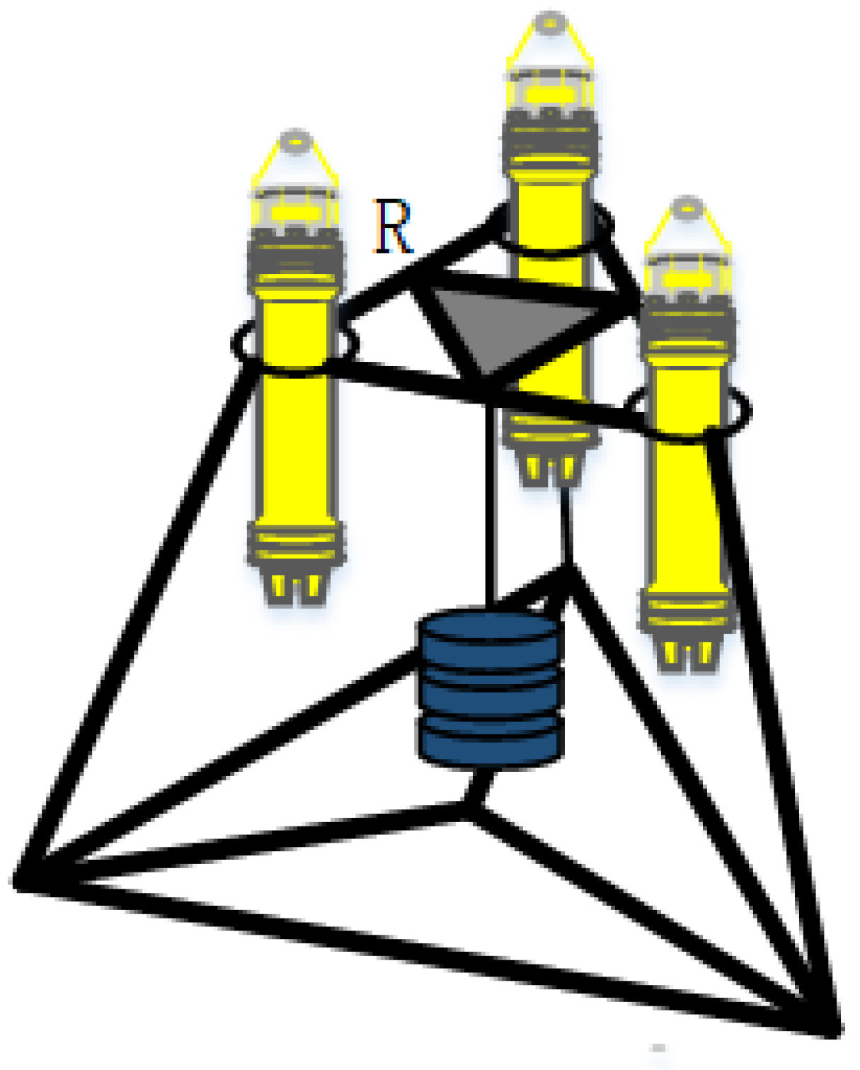
Figure 2.
seafloor geodetic station physical map and structure description.
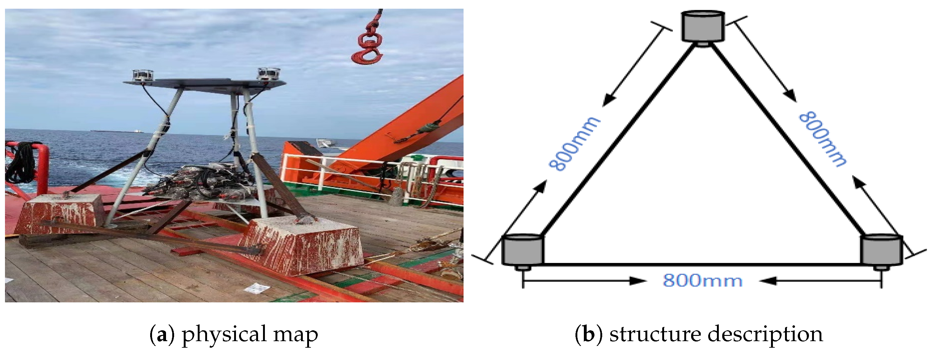
Figure 3.
Observation trajectory when the test ship locates the acoustic beacon.
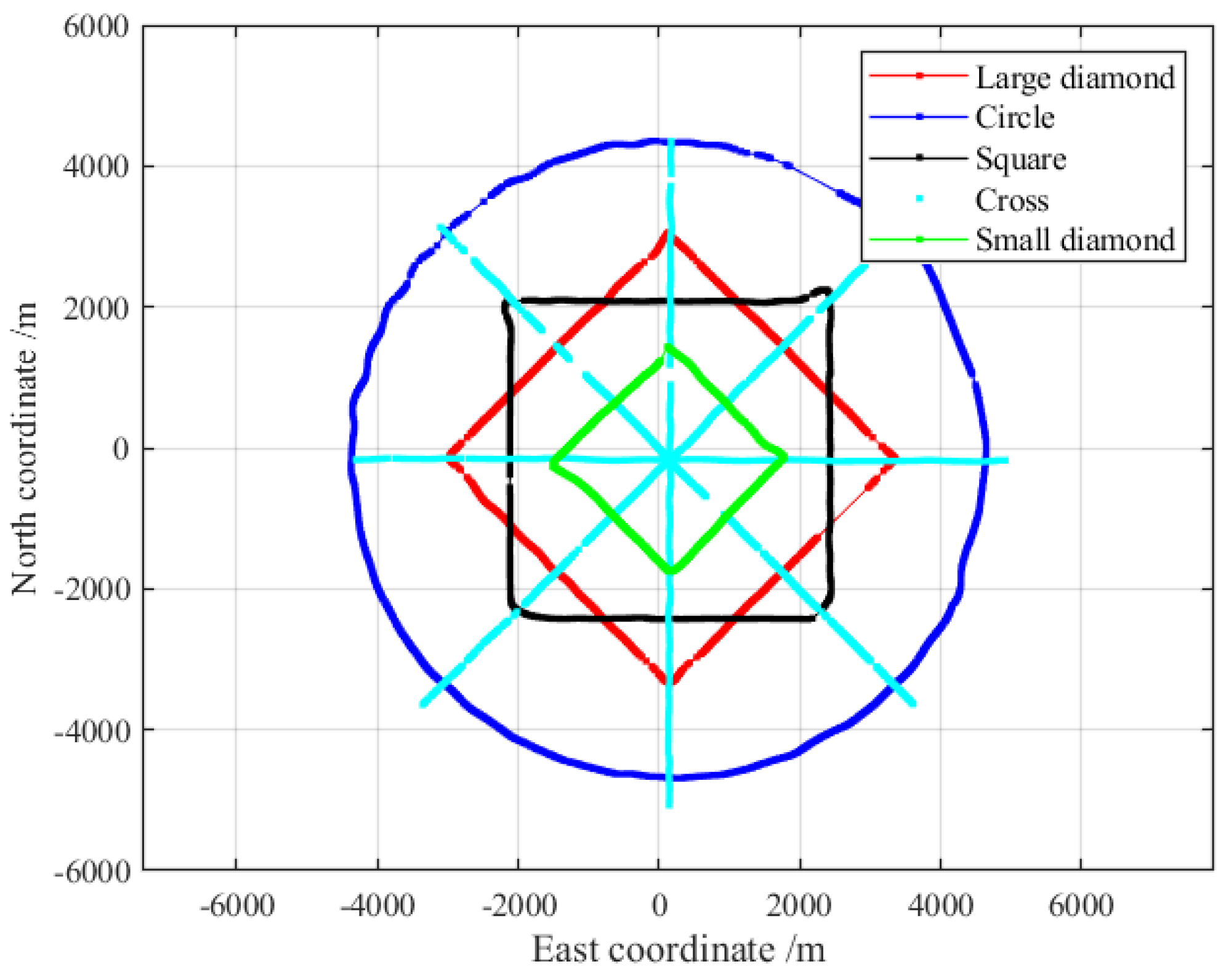
Figure 4.
Acoustic beacon positioning accuracy analysis.
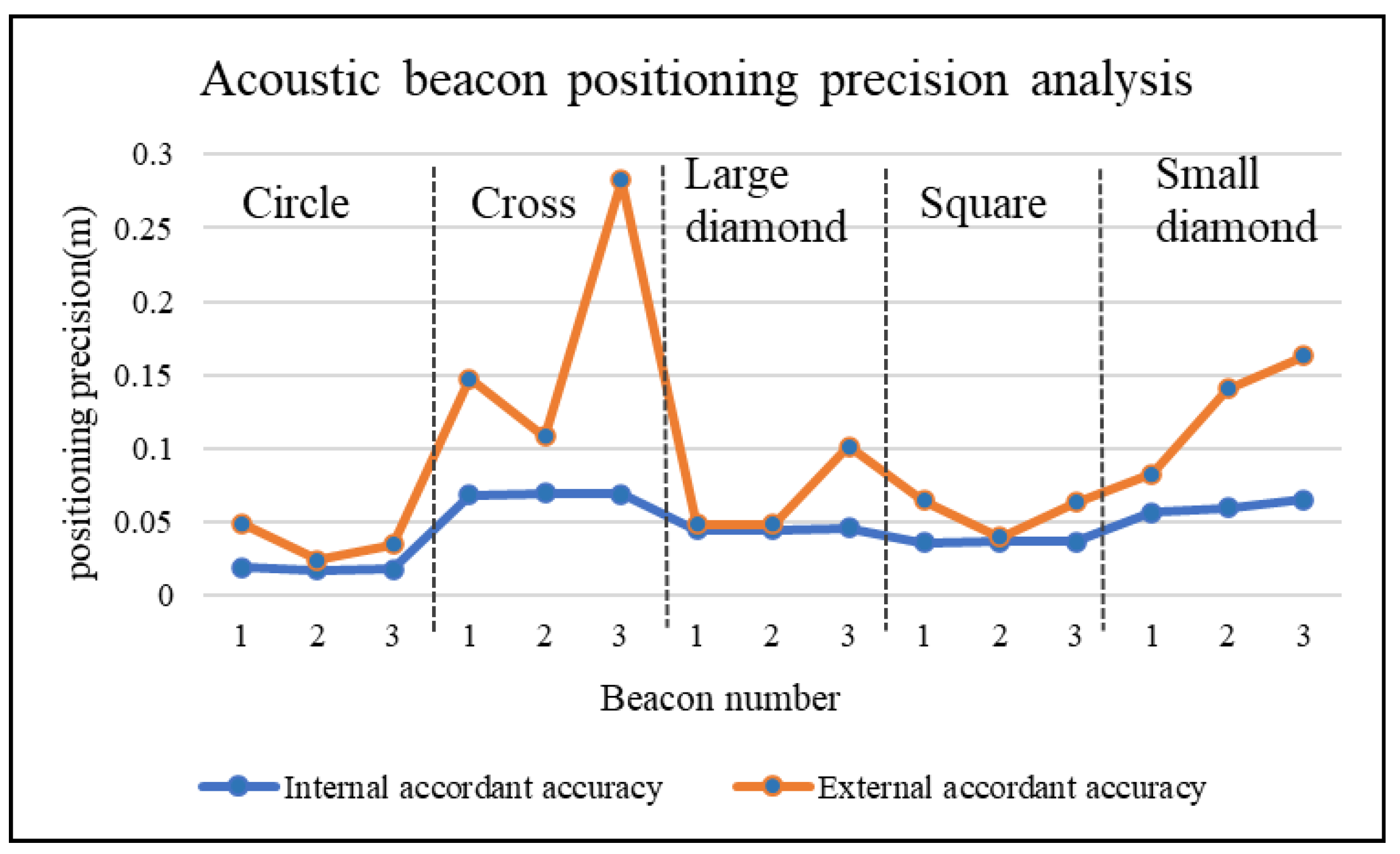

Table 1.
Comparison of positioning results of different observation strategies.
| Observation Trajectory | Beacon Number | North Coordinate (m) | East Coordinate (m) | Elevation (m) |
|---|---|---|---|---|
| Circle | 1 | 0.5195 | −0.4822 | −0.200 |
| 2 | 1.2382 | −0.2153 | −0.129 | |
| 3 | 1.0951 | −1.0095 | −0.137 | |
| Cross | 1 | 1.2671 | −0.1215 | 2.862 |
| 2 | 1.8375 | 1.6804 | 2.870 | |
| 3 | 1.7036 | −0.5058 | 2.937 | |
| Large diamond | 1 | 1.2609 | −0.0200 | 3.499 |
| 2 | 2.0535 | 1.7783 | 3.421 | |
| 3 | 1.9166 | −0.5626 | 3.416 | |
| Square | 1 | 1.1502 | −1.1955 | 1.001 |
| 2 | 1.8704 | −0.9398 | 2.897 | |
| 3 | 1.7664 | −1.7356 | 2.891 | |
| Small diamond | 1 | 1.0900 | 1.5812 | 2.333 |
| 2 | 1.8114 | 1.3134 | 2.254 | |
| 3 | 1.6363 | −0.0102 | 2.233 |
Disclaimer/Publisher’s Note: The statements, opinions and data contained in all publications are solely those of the individual author(s) and contributor(s) and not of MDPI and/or the editor(s). MDPI and/or the editor(s) disclaim responsibility for any injury to people or property resulting from any ideas, methods, instructions or products referred to in the content. |
© 2024 by the authors. Licensee MDPI, Basel, Switzerland. This article is an open access article distributed under the terms and conditions of the Creative Commons Attribution (CC BY) license (http://creativecommons.org/licenses/by/4.0/).
Copyright: This open access article is published under a Creative Commons CC BY 4.0 license, which permit the free download, distribution, and reuse, provided that the author and preprint are cited in any reuse.


