Submitted:
01 October 2024
Posted:
01 October 2024
You are already at the latest version
Abstract
In the study of mountainous areas, mountain peaks play a vital role as geomorphic features that have significant influence on hydrological processes, vegetation distribution, and other important topographic characteristics. From the perspectives of geomorphology and hydrology, the river network water system is an interconnected entity that serves as a crucial component in describing regional topography, geomorphology, and hydrological features. The primary objective of this article is to extract water system information and mountain peak data in Chongli District, Hebei Province. To extract mountain peaks, coarse-resolution Digital Elevation Model (DEM) data is utilized to estimate their positions and initiate data sampling based on DEM elevations. Deep learning models are employed to avoid explicit feature extraction and instead implicitly learn from training data. By using weight sharing techniques, the training parameters of the network are reduced, achieving more accurate extraction and recognition of mountain peaks in Chongli District, along with their classification. For the extraction of the water system, the fast regional convolutional neural network algorithm from target detection is introduced to enhance the efficiency and accuracy of extracting water system information through image processing. This algorithm rapidly identifies the type, location, and width of the water systems. Additionally, the AlexNet transfer learning method is applied to locate the river skeleton within the extracted water system area. Morphological methods are then used to extract river morphology and calculate its length and width. Finally, a developed algorithm for water system information extraction detects the presence of water system coverage areas in Chongli District. Through experiments, a total of 2792 mountain peak data points were successfully extracted. In terms of water system information extraction, the Faster R-CNN and CNN-based methods demonstrate high efficiency and low detection rates. This study provides information services and data support for the operation and maintenance of the Chongli Winter Olympics. Furthermore, it serves as a reference for future research conducted by scholars in the Chongli area, offering insights into various fields such as environmental changes, vegetation classification, and geomorphic features.
Keywords:
peak point
; Water System
; DEM
; Spatial Analysis
; GIS
; terrain characteristics
; Landform
; Error Analysis
; Deep Learning
1. Introduction
Forests are integral to the Earth's ecosystems, playing a pivotal role in climate regulation, biodiversity conservation, and water cycle maintenance [1]. The intricate relationship between forest ecosystems and geomorphological features necessitates a comprehensive understanding to inform effective forest management and conservation strategies. This study aims to bridge the gap between forestry knowledge and the recognition of mountain topography and water systems, leveraging the power of deep learning to enhance our ability to analyze and interpret complex terrain data.
In the contemporary era, the integration of modern informatization tools has revolutionized the field of forestry and geospatial analysis. Advanced technologies such as remote sensing, geographic information systems (GIS), and artificial intelligence (AI) have become indispensable for collecting, processing, and interpreting vast amounts of spatial data. These tools not only facilitate the precise mapping of forest canopies and the monitoring of forest health but also enable the detailed analysis of terrain features, leading to more informed decision-making in forest management and conservation efforts. The advent of high-resolution digital elevation models (DEMs) has marked a significant advancement in terrain representation, providing a detailed account of the Earth's topography and enabling the calculation of various morphological attributes foundational for environmental and topographical studies. Furthermore, the application of deep learning algorithms has introduced a new paradigm in the automated extraction of features from DEMs, offering unprecedented accuracy and efficiency in the recognition of complex terrain patterns.
Historically, the portrayal of the Earth's surface has evolved from rudimentary sketches to sophisticated digital representations, with digital elevation models (DEMs) marking a significant advancement in terrain representation [2]. DEMs provide a de-tailed account of the Earth's topography, enabling the calculation of various morpho-logical attributes that are foundational for environmental and topographical studies [3]. However, the full potential of DEMs is realized when complemented with forestry knowledge, which offers insights into the spatial distribution of vegetation and its im-pact on hydrological processes.
DEM has been widely applied in various fields, mainly because DEM has constant accuracy and multiple expression methods. For instance, DEM (Digital Elevation Model) is an important factor in classifying forest vegetation distributed by elevation. Combining spectral information with elevation data is very useful for object recognition and classification [4]. This method can enhance the accuracy of forest type identification, especially in areas with complex and variable terrain such as mountainous regions. By analyzing spectral characteristics at different elevations, it is possible to more accurately distinguish between different types of forest vegetation, as they may exhibit varying growth patterns and spectral reflectance characteristics at different heights [5]. DEM is an important component of spatial data infrastructure, with the rapid development of science and aerospace technology and the popularization of geographic information systems, DEM data contains a wealth of earth science information related to terrain and landforms.
The texture of digital elevation model (DEM) images, which vividly captures variations in texture, serves as a crucial dataset for reflecting surface characteristics and classifying landforms [6]. As a new type of digital map, DEM has unparalleled advantages. For example, DEM is used in forest planning, traffic route planning, surface statistics and analysis, and terrain analysis [7]. DEM contains a large amount of geological information and serves as fundamental data for quantitatively describing spatial changes such as landform structures, hydrological processes, and spatial distributions. Key points on the terrain surface can be extracted from the DEM, assessed not only by their local relief but also by their significance in identifying the inherent geomorphological and topographic features within the DEM [8]. However, DEM is essentially discrete elevation data, and each data point alone cannot truly reflect the complex and ever-changing surface morphology. Therefore, terrain analysis of DEM requires a technology that can extract terrain attributes and features based on the Digital Elevation Model, namely Digital Terrain Analysis (DTA). In the book "Digital Terrain Analysis"[9], Zhou Qiming and Liu Xuejun summarize the applications of digital terrain analysis into several aspects: hydrology, geomorphology and soil science, ecology, geographical information systems.
In terms of hydrology [10], DEM can be used to simulate water flow paths and accumulation, thereby evaluating flood risks and river hydraulic conditions. DEM provides an efficient method for representing the ground surface and enables the automated direct extraction of hydrological features [11], By analyzing watershed characteristics and slopes in DEM [12], the spatial distribution of hydrological units and elements can be determined, providing a basis for water resource management and flood control engineering. Automated extraction of hydrological parameters from DEMs offers quicker processing times, reduced subjectivity, and enhanced reproducibility compared to manual methods (Tribe 1992; Garbrecht and Martz 2000; Starks et al. 2003) [13,14,15,16]. DEMs are extensively employed in the simulation of surface hydrological processes. Their applications encompass the automated identification of watershed boundaries, the characterization of topographical features for hydrological and soil moisture estimation, and the mapping of drainage systems [17].
In the fields of geomorphology, soil science, and ecology [18], DEM can be used to extract terrain features such as mountains, rivers, and valleys, and analyze their spatial patterns and terrain parameters. Recent studies indicate that DEMs are utilized for change detection, aiming to map or monitor erosion, deposition, volumetric changes, and to establish sediment budgets [19]. These terrain parameters can be used to study ecological processes such as soil erosion, vegetation distribution, and species diversity, providing scientific basis for ecological environment protection and restoration. In the study, a top-down hierarchical approach combined with coarse DEM information can be employed for forest mapping in large, steep mountainous areas to understand the local ecological conditions [20]. Carrying out this approach is essential for ecological modeling of processes influenced by landscapes, including the sequestration of atmospheric carbon, soil erosion, and denitrification. It also aids in the strategic planning and implementation of soil management practices that are both environmentally beneficial and economically viable [21].
In the application of Geographic Information Systems (GIS), DEM [22], as fundamental data, can be integrated and analyzed with other spatial data, such as map overlay, visualization analysis, and route planning. Using Geographic Information Systems (GIS) to conduct quantitative analyses of Digital Elevation Models (DEM) across various models enables users to extract a wide array of landscape information, focusing on critical hydrological and topographic data [23]. By combining DEM with other geographic data, spatial analysis and decision support can be conducted, providing spatial information solutions for various industries. For instance, the integration of GIS and DEM enables the identification of hierarchical vegetation cover units, classes of vegetation cover, and predominant woody species within satellite imagery. The characteristics depicted in the DEM serve as indirect indicators of the conditions at vegetation sites. Parameters of morphometric relief and complex ecological features derived from DEM are utilized for the automated classification of DEM data [24].
The integration of modern informatization tools has revolutionized the fields of forestry and geospatial analysis. For instance, PointDMIG offers a robust spatial clustering framework, which is designed to detect enduring spatial relationships among point cloud sequences, all the while maintaining the integrity of spatial data [25]. It can be adapted to identify patterns in forest coverage and topographic features. VDTN, by leveraging its capability to enhance vector data, integrates an innovative multi-copy routing algorithm, ensuring the highest likelihood of successful message delivery across all movement models and being applicable to various message generation intervals [26]. This can be utilized for the acquisition of DEM data to maintain its high fidelity and optimize the computational process. Furthermore, the KNN-based model has achieved higher predictive accuracy in short-term traffic forecasting than other models [27], and it can be used to infer the short-term dynamics of forests and fluctuations in water systems.
As we venture into the era of smart forestry, the challenge lies in harnessing these technologies to strike a balance between commercial exploitation and ecological preservation. The potential of machine learning and artificial intelligence (AI) in predicting forest growth patterns, optimizing timber yields, and preserving biodiversity is immense. These tools can analyze vast datasets to identify trends and anomalies, providing actionable insights that were previously unattainable. For example, in terms of offering adaptable and extensive connectivity, Unmanned Aerial Vehicles (UAVs) have been widely deployed as effective aerial base stations (BS) to complement cellular networks. In some studies, Mobile Vehicles (MVs) and UAVs are jointly utilized for energy replenishment and data collection, capitalizing on the UAV's flexibility and high efficiency, as well as the MV's stability and low cost [28,29]. The deployment of unmanned aerial vehicles (UAVs) for precision forestry will lead to more accurate inventory assessments and habitat monitoring, minimizing human interference and ecological disruption. The CTC algorithm is rapidly developing, enabling coexistence of various technologies within the same frequency band, allowing direct communication between different wireless technologies, promoting the efficient use of spectrum resources, thereby preventing interference and enhancing the overall utilization rate of the spectrum. Moreover, CTC can predict potential failures and carry out repairs and management in advance. [30,31,32,33]. Leveraging these capabilities, CTC can become an invaluable tool for processing time-series data from forestry sensors and remote sensing data, thereby simplifying the process of identifying forest growth patterns and ecological changes over time. Besides, 2D LiDAR SLAM technology is a method capable of providing high-precision, real-time environmental data. When integrated with IoT devices, it can capture point clouds of the canopy, offering a comprehensive understanding of the physical structure of the forest and its changes over time [34,35]. The development of decision support systems powered by AI will be crucial in optimizing resource allocation, guiding reforestation efforts, and ensuring the long-term viability of forest ecosystems.
In recent years, deep learning has shown significant promise and efficacy in assessing forest resources, playing a crucial role in understanding and managing these resources and their ecosystems [36]. Notably, deep learning models have made breakthroughs in blind image deblurring, which can be instrumental in enhancing the analysis of forest canopy and terrain features from remotely sensed images [37]. Using digital maps to represent spatial information about the terrain replaces the traditional labor-intensive manual mapping, not only making geographic information clear briefly but also making the application of topographic maps more flexible [38]. By integrating these advanced informatization technologies with traditional forestry knowledge, we can achieve a more nuanced understanding of forest ecosystems and their interactions with the terrain. This integration not only enhances the accuracy of mountain peak and water system recognition but also lays the foundation for developing predictive models that support proactive forest management and conservation efforts.
This paper presents a novel approach to extract water system information and mountain peak data in Chongli District, Hebei Province, by utilizing coarse-resolution DEM data and deep learning models. We employ weight sharing techniques to reduce training parameters, achieving more precise extraction and recognition of mountain peaks. Furthermore, we introduce a fast regional convolutional neural network algorithm to enhance the efficiency and accuracy of water system information extraction through image processing. Our approach involves an innovative application of Convolutional Neural Networks (CNNs) for the identification of mountain peaks and water systems, utilizing high-resolution data provided by Digital Elevation Models (DEMs). CNNs, a class of deep learning algorithms, are particularly adept at image recognition tasks and were selected for their exceptional performance in processing complex spatial data. CNNs are widely applied, and in the future, we can also leverage the conversion of Wi-Fi Channel State Information (CSI) into CSI-Gramian Angular Field (CSI-GAF) images, combined with the powerful feature extraction capabilities of 2D-CNNs to gain actionable insights. This conversion not only enriches the data representation for 2D-CNN analysis but also enhances the network's ability to discern subtleties in the spatial distribution of forest canopies, the delineation of water networks, and the recognition of topographic features [39]. The integration of forestry knowledge with deep learning models provides insights into environmental changes, vegetation classification, and geomorphological features, contributing to a broader understanding of the interactions between forest ecosystems and topographical characteristics.
2. Materials and Methods
2.1. Overview of the Study Area
Considering the richness of landform types and the availability of experimental data, the research area is mainly selected in Chongli District, Hebei Province. Chongli District, the administrative district belongs to Zhangjiakou City, Hebei Province. Its geographical location (see Figure 1, collected on August 25, 2020) is 40°47′-41°17′N, 114°17′-115°34′E. The area is 2334 square kilometers, the altitude is 813-2174m, and the maximum height difference is 1361m. On-site observation data show that the average daily maximum temperature in this area is 12°, and the average daily minimum temperature is -2°. The total volume is 100.69 million cubic meters.
From the perspective of topography, 80% of the territory is mountainous, and the forest coverage rate reaches 52.38% [40]. There are mainly Paleozoic and Proterozoic strata in the territory, and Mesozoic and Cenozoic strata are sporadically exposed in some areas and intermountain valleys. The territory is the mountainous area in the northwest of Hebei Province, which belongs to the intersection zone of the eastern section of the Yinshan Mountains to the branch of the Damasan Mountains and the remaining veins of the Yanshan Mountains, mostly in the direction of northeast-southwest and east-west. The landform is a transitional mountainous area above the dam and below the dam. The mountains are steep, and the peaks are mostly between 1500 meters and 2000 meters above sea level, which belongs to the middle and low mountainous areas. The altitude of Chongli District is 813-2174 meters above sea level, and the maximum height difference is 1361 meters.
From the perspective of climate characteristics, the climate in Chongli District belongs to the temperate sub-arid zone of East Asia continental monsoon climate. Due to the influence of geographical location and terrain, the air activity is frequent in winter, and the temperature rises quickly in spring, but the temperature fluctuates greatly, the frosting period is late, the rainfall is relatively small, and the number of windy days is more. The summer is cool and short, the temperature is relatively stable, the temperature difference between day and night is large, and the rainfall is concentrated. Due to the terrain of the mountainous area, there are occasional hail and rainstorm disasters; the temperature drops rapidly in autumn, and the first frost appears earlier. The distribution of average temperature in Chongli District is greatly affected by topography and topography. The isotherm is basically northeast-southwest, and the northern part of Shancha, Dashuiquan, Shiyaozi, Shizigou, Qingsanying and Sitaizui Township near Batou has an annual average temperature of 0-20°C, which is consistent with the contour The lines match. The average summer temperature in Chongli District is 19°C, and the concentration of negative oxygen ions in the air reaches 10,000 per cubic meter, which is more than 10 times higher than that in urban residential areas. The average value of PM2.5 is better than the national first-level standard. The average temperature in winter is -12°C, the average wind speed is only grade 2, the snow falls early, the snow is thick, and the snow storage period is long. The annual snow accumulation is about 1.5 meters, and the snow storage period is more than 150 days. The average precipitation over the years is 483.3 mm, and the average temperature over the years is 3.7°C.
From the perspective of water system hydrology, the surface in Chongli District is mainly precipitation, with an annual average water volume of 488 mm and a total precipitation of 1.13 billion cubic meters; the average annual runoff of the surface water in the whole region is 42.9 mm, and the total annual runoff is 100.69 million cubic meters rice.
2.2. Overview of the Study Area
2.2.1. Selection of Data Source
Digital Elevation Model (DEM) is a discrete digital representation of ground elevation. Through elevation data, researchers can easily obtain information such as elevation, slope, and aspect of the research area. The DEM used in this study comes from the Advanced Land Observing Satellite (ALOS) of the Japan Aerospace Exploration Agency (JAXA), which is equipped with a Panchromatic Remote-sensing Instrument for Stereo Mapping, PRISM), Advanced Visible and Near Infrared Radiometer type 2 (AVNIR-2) and Phased Array L-band Synthetic Aperture Radar (Phased Array L-band Synthetic Aperture Radar, PALSAR) has a total of three sensors. The satellite was launched on January 24, 2006, and ceased to be used on April 22, 2011, but as of the time of this study, the necessary data are still available through the official website of the Alaska Satellite Facility (ASF) . The DEM data used this time is generated by the all-weather observation data of the PALSAR sensor of ALOS. The terrain resolution obtained by the PALSAR sensor is divided into two types. The actual resolution of the directly downloaded DEM data is . Compared with other mainstream DEM products, ALOS has the advantages of higher resolution and finer texture features, which provides more opportunities for the construction of biomass inversion models.
Due to the influence of spatial resolution and system error, some erroneous "depressions" will be generated during the generation of DEM data, which will cause incorrect flow direction of depressions in DEM when river flow direction is extracted, which will affect the river network Extraction accuracy. Therefore, the original DEM needs to be "filled" to remove the influence of the depression. But not all depressions are caused by data errors. Some depressions are the response of real terrain. Based on this theory, when the original DEM is "filled", a reasonable filling threshold should be set to obtain the final initial data. .
2.2.2. Sample Area DEM Data Acquisition
In the field of geographic information, contour topographic maps mainly reflect the geomorphology of mountain elements, and it is difficult to accurately describe the spatial elevation changes of topographic elements in the form of images. The digital image reflects the elevation change of the mountain with multi-level grayscale differences through grayscale rendering of DEM data. Therefore, in order to effectively use the deep network for terrain feature extraction in DEM data, the contour image is used to reflect the topography of the mountain data, and the grayscale rendering image is used to represent the elevation change trend in the mountain data. The generation and gray-scale rendering processing, as shown in Figure 3, combines the features of the mountaintops in the two modes in the form of image synthesis, and then forms the learning sample data that the deep network can receive.
For the extraction of mountain tops, this paper uses the DEM data provided by ASTER GDEM (Advanced Spaceborne Thermal Emission and Reflection Radiometer Global Digital Elevation Mode) as the basic data. First, select the mountain part according to the elevation distribution, and cut out 1000 pieces with a size of 320* 320 mountain data blocks, ensure that there are at least one or more mountain tops in each data block, and preprocess the DEM data according to the method in Figure 3. At the same time, the minimum circumscribed rectangle method is used to mark the mountaintop area in the superimposed image to ensure that there is only one mountaintop in each marked rectangle, and contain as little background information as possible, forming the mountaintop sample data as shown in Figure 4. Among them, Figure 4 is the superimposed mountain contour rendering; Table 1 is the label information of the sample, which are the coordinates of the lower left corner (x1, y1) and the coordinates of the upper right corner (x2 ,y2) and lable label. Finally, the learnable sample set PEAK-100 containing the mountain top target area was established, including 3500 mountain top samples, and the mountain top sample set was divided into training set, verification set and test set according to the ratio of 6:3:1.
For the extraction of the water system, this paper uses the elevation data provided by ASTER GDEM in this paper, and preprocesses the downloaded data such as data mosaic, coordinate conversion, and data clipping to obtain the original DEM image of the same size as the research area. ASTER GDEM is the most commonly used One of the surface digital elevations, it is widely used in the research of water system information extraction.
Due to the influence of spatial resolution and system error, some erroneous "depressions" will be generated during the generation of DEM data, which will cause incorrect flow direction of depressions in DEM when river flow direction is extracted, which will affect the river network Extraction accuracy. Therefore, the original DEM needs to be "filled" to remove the influence of the depression. But not all depressions are caused by data errors. Some depressions are the response of real terrain. Based on this theory, when the original DEM is "filled", a reasonable filling threshold should be set to obtain the final initial data.
2.3. Extraction of Mountain top Points Based on DEM and Deep Learning
2.3.1. Definition of Mountain Top Point
2.3.1.1. The definition of Mountain Vertex in Geomorphology
Geographically, a mountain refers to a highland with a steep slope, generally with an altitude greater than 500m and a relative relief of more than 200m. The mountain top generally refers to the highest point of the mountain, and also refers to the maximum point of the elevation value in the local area, that is, the local jump point [0 of the ridge line, which is one of the important topographic feature points.
From the point of view of landform, the top of the mountain must be the highest point in the local area, but the point with the highest value in the local area is not necessarily the top of the mountain. Geographically, the vertices are generally distributed in a point group mode, and the points are both independent and related to each other and have a hierarchical structure.
2.3.1.2. Definition of Mathematical Model of Mountain Top Point
In 2002, based on the contour model and the analytical expression of the terrain, Zhong Yexun made a mathematical definition of the topological shape of the mountain top based on topological rules. The main idea of its definition is: Let the terrain surface be T, a and b be any two points on T, and their elevations are Ha and Hb respectively. For any point i on T, if the following conditions are met:
In the formula, Bi is the plane passing through point i, CMi is the contour line passing through i, and T is the hillside surface with b as the top. CMa=Ma T is the contour line at the foot of the mountain, and the points satisfying the point set TM= {CMi, i<[a,b]} constitute the hillside TM.
If CMi=Mb T, T is the sharp point.
If Ma T <CMi<Mb T, T is the dome.
When b∈S∈T and for any b∈S, there exists=c (c is a constant), then T is a mesa with S as the top of the mountain. Among them, ES, CVS and CNS represent equal slope, concave slope and convex slope, respectively.
If the terrain surface T is expressed as:
If the terrain surface T is expressed by a polynomial in the form of Equation 2, when any point p (x, y) satisfies the following conditions, then it is judged that P is the top of the mountain:
If β=0; maximum curvature C_max>0; and minimum curvature
C_min>0
The coefficients in the polynomial shown in Equation 2 satisfy:
2.3.1.3. Definition of mountain vertex in grid DEM
The grid DEM uses a discretized regular grid to describe the surface relief state, and each grid records the elevation attribute of the ground surface. Therefore, for the grid DEM, due to the regularity of the square grid, the plane position of the grid point (x, y) is implicitly not recorded in the row and column numbers i and j of the grid, and the DEM is equivalent to an elevation matrix with m rows and n columns, which can be expressed as,
The summit is geometrically the highest point of the mountain. Therefore, in the DEM, the mountain point can be considered as the highest point in a certain area S according to its geometry, that is:
In the DEM, the peak of the mountain can be ideally represented as shown in Figure 5.
2.3.2. Extraction of Mountain Top Point
Based on the low accuracy of the traditional mountain top extraction method, this paper proposes a geomorphological classification method to obtain the minimum elevation threshold of the mountain top in Chongli District through the factors of altitude and fluctuation and uses ResNet-101 as the feature extraction of the mountain top recognition model. Network, obtain the anchor frame setting suitable for the identification of the mountain top area, automatically generate a high-quality mountain top target area, and finally combine the elevation calculation to realize the mountain top extraction and recognition technology for accurate extraction of the mountain top.
2.3.2.1. landform Classification
Table 2 is the principle for the classification of landform types in China and its adjacent areas jointly produced by the Nanjing Institute of Geography and Limnology of Chinese Science of Science, and nine units including the State Oceanic Administration and the Chinese Academy of Sciences.
Undulation refers to the relative change in elevation of the area, which is the standard deviation defined mathematically. Therefore, for the raster data with a size of m×n, the calculation method of the undulation of this area is Eq.7, which represents the elevation value of the grid point. Represents the average elevation value of the area. Based on the above theoretical support, the basic geomorphology of Chongli District is divided step by step through the two indicators of surface relief and altitude. The altitude distribution map of Chongli District is shown in Figure 6, and the topographical relief map is shown in Figure 7. The terrain division of Chongli District is shown in Figure 8 by combining Table 2 and Eq.7. We will obtain the division results and Chongli Comparing the results of the second actual survey of the Li District, the division results are in line with the actual situation of the Chongli District.
Combined with previous analysis of China's actual landforms (Li Bingyuan et al., 2008), the Qinghai-Tibet Plateau and the Yunnan-Guizhou Plateau belong to extremely high mountainous areas; the Loess Plateau belongs to hills and mountains; the Sichuan Basin belongs to hills; other plain areas have fewer and Relatively independent, combined with Figure 6 and Eq.8 to summarize the criteria for the division of geomorphic types and the setting principles for the minimum elevation of the mountain top (Table 3).
Determined minimum elevation thresholds for mountain apexes in Chongli District
2.3.2.2. Peak point Extraction Algorithm
In order to obtain more mountain top features in mountain samples and extract the coordinate position of the mountain top more accurately, this paper designs a mountain top recognition framework implemented by ResNet-101 residual network under Keras. First, use the feature extraction module to deeply mine the morphological features of the mountain top area in the mountain sample, and then combine the core RPN network module of Faster R-CNN to automatically generate a high-quality mountain top target area, and finally map the mountain top target area in the sample image back to the original In the DEM data, the position of the maximum elevation value in the target area is calculated as the final coordinates of the mountain top.
The extraction of mountain top features plays an important role in identifying mountain tops. To improve the recognition effect of mountain top areas, according to our inertial thinking, the deeper the network layer is, the better the learning ability of the network should be. As the number of network layers increases, the effect of the network first becomes better to saturation, and then immediately declines. In order to solve the problem of gradient degradation and extract the deep-level morphological features of the mountaintop area, build a ResNet-101 network under Keras and construct a residual block (Residual block) to complete, and the unknown function H(x) that needs to be learned to approximate Identity mapping becomes a function that approximates F(x)=H(x)-x, and the residual module has two convolution layers represent two in the second convolution operation, x is the input value of the residual block, F(x) is the input value of the convolution block, and F(x)+x is the output of the residual block. Considering the limited sample data of mountain tops in the self-built Chongli District, and the performance of the convolutional neural network is affected by the number of samples that can be learned, by referring to the ideas of literature [41], firstly, through the ImageNet dataset. The ResNet-101 network model performs pre-training, freezes the extracted bottom-level convolutional blocks about the general features of the thousand layers, and then fine-tunes the internal parameters of the top-level convolutional blocks by using the self-built mountain peak samples, and performs current training through transfer learning. Feature extraction for mountain vertices.
Use the RPN module to search for possible target mountaintop areas in mountain samples. RPN performs spatial convolution on the feature map in the form of sliders, selects deeper features in the mountaintop area, and maps each pixel on the obtained spatial convolution map. Return to the position of the original mountain sample and generate anchor boxes with different sizes and ratios. The original method uses the default anchor frame parameters to achieve accurate identification and positioning of the mountaintop area. However, in order to improve the recognition accuracy of the mountaintop pixels, the mean shift clustering algorithm is firstly used to set the anchor frame parameters suitable for the mountaintop target area according to the mountaintop labeling samples. , where the main idea of the mean shift clustering algorithm is based on the sliding window algorithm to find the dense area of data points, and then based on the centroid, update the candidate point of the center point to the mean value of the points in the sliding window to complete the positioning of each group /class center point, and then remove the similar windows of these candidate windows, and finally form the center point set and the corresponding grouping. Here, the size of the label box in the self-built hilltop training set is used as the input of the clustering algorithm, and the sample set is collected. Cluster analysis is performed on the labeled boxes to determine the anchor boxes that are finally used for mountain apex recognition.
In order to filter the generated anchor boxes, the intersection ratio between the anchor box and the marked box in the hilltop area can be calculated, set >0.6 as foreground threshold, set <0.4 as background threshold,In this way, the acquired anchor frames can be divided into foreground thresholds that contain mountain vertices and background thresholds that do not contain mountain vertices, discard anchor frames that are in the middle threshold, and use the non-maximum suppression method NMS (Non-Maximum suppression, The NMS) method screens the candidate frames, sorts the remaining anchor frames according to their reliability, and retains the candidate frames with a higher probability of containing mountain vertices, so as to achieve a rough estimation and positioning of the mountain vertices in Chongli District. The method to calculate is shown as Eq.9,and Indicates the anchor box,is the marker box for the hilltop;Eq.10 indicates the center coordinates and length and width of the anchor box, also indicates the center coordinates and length and width of the anchor box.
Finally, after obtaining the candidate area of the mountain top through the RPN network module, it is necessary to identify and correct the candidate area with the help of a classification regression network. Due to the different sizes of the anchor boxes in the candidate area, to further screen and identify the mountain tops, it is necessary to input the final classification layer and regression layer calculation after the maximum pooling and output the probability value of each candidate box conforming to the mountain top characteristics. Finally, in order to accurately mark the mountain top area in the obtained mountain top area, map the mountain top target area identified in the mountain image to the original DEM data, obtain the elevation value of each coordinate in the mountain top area through the Arcgis10.8 platform, and calculate the elevation in the area The exact coordinates of the peak of the mountain can be marked at the maximum value point, and the calculation method is shown in Eq.11, is the position of hilltops,is the elevation of the position of(i,j).
2.3.2.3. Recognition Algorithm of Mountain Top Point
After obtaining the information on the top of the mountain in Chongli District, it is necessary to further identify the type of the top of the mountain. According to the analysis of the top of the mountain, the top of the mountain can be divided into three types: (1) The top of the mountain is sharp and point-like, and the area of the top of the mountain is small. (2) Round mountain top: The top of the mountain has a large area, and the overall shape is relatively smooth. (3) Flat mountain top: the surface of the top is flat, and it is difficult to determine the position of the top of the mountain. First, determine the highest connected domain where the mountain top is located and calculate its area S, and judge whether S is smaller than a given minimum threshold. If so, it means that the shape of the mountain top is sharp and point-like, and the area of the mountain top is small, which is a sharp mountain top. Otherwise, it is necessary to further judge whether it is a round mountain top or a flat mountain top. Then, by calculating the undulation of the peak that does not meet the requirements of the sharp peak, it is judged whether it is less than a given minimum threshold. If yes, it is judged to be a flat-topped mountain, otherwise it is a round-topped mountain.
2.4. Water system Information Extraction in Chongli District Based on Faster R-CNN
The water system identification process is shown in Figure 10. At present, there are various methods for collecting apparent images of water systems, such as unmanned aerial vehicles, professionally equipped cameras, and remote sensing image data, all of which can achieve fast, non-contact, high-quality data collection. Preprocess the collected data, including cropping and segmentation of water system pictures, unify the size and enhance picture data; then classify according to the type of water system, use special software to mark the images, and establish a corresponding sample database; after that, the sample data used for training Input it into the constructed Faster R-CNN network, and perform deep learning on the entire network by adjusting the parameters; finally, test the trained network. For the identified water system, after the algorithm determines its bounding box, it further refers to the AlexNet transfer learning in CNN and combines the morphological algorithm to perform subsequent processing on the water system, extract the shape of the water system, and obtain the length and width of the water system in the image of the water system, so that Water system information is more accurate and abundant.
2.4.1. System Architecture
2.4.1.1. Faster R-CNN
The Faster R-CNN algorithm is derived from CNN and is an advanced version of the target detection algorithm R-CNN and Fast R-CNN, which has a significant improvement in speed and demonstrates superior ability in locally discriminating features. [42,43]. When modeling global spatiotemporal information from video data, CNN models often rely on local spatiotemporal convolutions between frames, with an emphasis on capturing local spatial features [44]. The architecture is shown in Figure 11. First, the image is input, and the image features are extracted through VGG16/ResNet. The advantage of ResNet is that the use of residual network can improve the recognition accuracy by increasing the depth, and the more layers of the network, the more abundant the features extracted at different levels. Then, on the generated convolutional feature map (Feature Map), the candidate window is generated through the region proposal network RPN and judged whether it is a foreground (target/water system). If the relevant area is classified as foreground, the water system will be classified through the fully connected layer, and the window coordinates will be fine-tuned through border regression. Finally, a rectangular frame will be used to mark the specific water system category on the output image, and its classification confidence will be given.
RPN belongs to the category of FCN (Fully Convolutional Networks). Its purpose is to obtain high-quality water system candidate area frames on the image, and replace the previous selective search method, so that the entire network can be trained end-to-end.
As shown in Figure 12, first, continue to apply 3×3 convolution on the feature map (generally 60×40 pixels in size and 256 dimensions in depth) output by the feature extraction network (ResNet, VGG, etc.), with the same size and depth, which is used to combine surrounding information to obtain a convolutional feature map. Then map each pixel on the feature map to the original image to generate 9 types of anchor boxes (Anchor).
At the same time, two convolution operations are performed simultaneously on the convolution feature map (the convolution kernel is 1×1), one of which is classified (divided into positive samples: target; negative samples: background), and each pixel outputs an 18-dimensional vector (9 anchor boxes × 2 classification scores); the other is regression, and the output is a 36-dimensional vector (9 anchor boxes × 4 coordinate values), so the final number of anchor boxes is: 60×40×9≈ 21600. Afterwards, suitable positive and negative samples are screened out through the following steps:
The(Intersection over Union) calculation (the ratio of the intersection and union of the area between the predicted anchor box A and the corresponding actual anchor box B) is shown in Equation 12, where the anchor box> 0.6 is regarded as a positive sample, and the< 0.4 is regarded as a negative sample, and the rest are discarded.
Non-Maximum Suppression NMS (Non-Maximum Suppression) is used to find the best detection target position by removing the anchor box with the highest coincidence rate with the true value, leaving only the candidate box with the highest predicted probability value as the final prediction result.
Rank sorting: sort the remaining anchor boxes from high to low in confidence, take at most the first 128 anchor boxes as the final positive samples for training, and provide 128 negative samples. Finally, the screened candidate boxes are substituted into the training network for training.
2.4.1.2. CNN-based water system identification
This section may be divided by subheadings. It should provide a concise and precise description of the experimental results, their interpretation, as well as the experimental conclusions that can be drawn.
The expansion area of the water system can be extracted through Faster R-CNN, which greatly reduces the detection range, and then CNN and sliding windows are used to identify the water system, and the specific location of the water system can be further determined.
The AlexNet neural network model is shown in Figure 14. The network consists of 5 convolutional layers and 3 fully connected layers, with a total depth of 8 layers. The output of the last fully connected layer is sent to the Softmax layer, as shown in Equation 14. Softmax It is possible to constrain the output to be in the range (0,1), thereby ensuring that the neuron is activated, resulting in a distribution covering multi-class labels. Compared with traditional neural networks, the Alex Net model has the following advantages:
1. Using ReLU activation function (Eq.13), if the input is not less than 0, the gradient of ReLU is always 1;
2. Enhance the dataset to suppress the fit;
3. Use the Drop Out method to suppress overfitting;
4. Use local response normalization layer to enhance generalization;
The input of the Alex Net model is 32*32*3. The pathological image used in this paper is a three-channel RGB image, and the dimensions meet the requirements of the model. After adjusting the size of the pathological image, it is sent to the network. First, it reaches the convolutional layer. After the first layer of convolution operation, the result is pooled, and finally it is normalized and then input to the second layer. Subsequent operations from the second layer to the fifth layer are similar to those of the first layer and will not be repeated here. The output of the fifth layer of the network will be sent to the subsequent fully connected layer. The outputs of the sixth and seventh layers are both vectors of length 1000. Finally, the network uses the Softmax classifier to obtain the final classification result.
AlexNet showed a good classification ability. At that time, because the training was very time-consuming, and secondly, the water system image dataset in this paper contains few samples, which is not suitable for deep network training of this scale. Therefore, AlexNet's migration learning (as shown in Figure 15) can be used to solve these problems.
This paper replaces the last three layers of AlexNet with a fully connected layer, a Softmax layer, and a classification output layer with the same number of nodes as the number of fault categories. Then, the entire structure will be divided into two parts: the retention layer and the replacement layer.
The parameters in the pre-trained network have been trained on ImageNet using millions of images, and the extracted features have been proven effective for classification. Only marginal adjustments to these parameters are required to adapt to new images.
Therefore, the parameters in the reserved layer will be retained and used as initialization, which can help the training to converge. The parameters in the replacement layer only account for a small portion of the entire network, allowing training with small datasets.
In this paper, Faster R-CNN has been used to identify the area where the water system expands in the form of an anchor frame. CNN has processed the basic skeleton of the water system. The boundary line of the background pixel gray scale is not obvious enough, so this paper introduces a morphological algorithm to perform subsequent processing on the coarse skeleton of the water system after CNN processing and restore the water system shape according to the minimum gray value in the bounding box area. The main steps are as follows:
1. Extract the minimum gray value pixel points of each column of the water system skeleton (CNN processing) in the bounding box area (Faster R-CNN processing) to form the initial basic skeleton of the water system.
2. Due to the influence of the surrounding geographical environment, the extraction results in the first step are prone to salt and pepper noise. In this paper, a 3*3 sliding window is used to traverse the image. If there is only one pixel inside the sliding window, the pixel in this area is filtered out.
3. Connected regions with smaller areas are filtered out by an area filter, and the adjacent connected regions are connected in the remaining connected regions.
4. Skeletonized water system form is convenient for extracting the width of the water system later. The skeleton obtained here is a complete continuous skeleton, which is different from the discontinuous skeleton obtained in the previous steps.
5. Combine steps 3 and 4 to extract the length and width of the water system. The width extraction method uses the traversal of the water system skeleton, and uses the normal length of the tangent line of each point on the skeleton as the water system width of the point, as shown in Figure 16, selects 30 points along the water system direction as the test points of the water system practice width, and the results show that the calculated The difference between the width and the actual width is 1-2m, and the average value of the width is used as the average value of the water system, and the error is within 5%.
3. Results
3.1. experiment preparation
Before the water system extraction experiment, the sample needs to be preprocessed. Because the original picture has problems such as insufficient light and low gray scale, the brightness and contrast of the picture can be adjusted to make the water system and the background more clearly distinguishable. This paper adopts the method of automatic color balance to adjust the contrast of the picture. This method mainly calculates the light and dark relationship between the target point and the surrounding pixels through difference and performs automatic pixel correction.
Due to the problems involved in sample labeling in supervised learning, the pictures in this paper are labeled with LabelImg. The labeling effect is shown in Figure 17. According to the degree of the water system, we can divide them into curved rivers and straight rivers, and according to the width of the river. For wide channels, the number of marked samples is 1320 for curved rivers (CC), 1520 for straight channels (SC), 645 for narrow channels (FC), and 525 for wide channels (WC).
3.2. experiment result
This study was carried out in the Keras deep learning development environment, and the self-built peak sample data set PEAK-100 was used for network training. The initial learning rate of the model was 0.002, the momentum was 0.8, and the number of iterations was 10,000. The initial size parameters of the anchor frame are set using the K-means clustering algorithm to set the marked frame in the training sample on the top of the mountain, and the width and height are calculated by the coordinates of the upper left corner and the lower right corner of the marked frame in the mountain top area, respectively, as the clustering algorithm. Data sample, let the criterion function of K-means clustering algorithm be:
In this formula: is a commonly used clustering criterion function, is the total number of samples of class j, is the sample mean of ,set=0.02 and =4 to carry on cluster analysis on training samples. According to the results of cluster analysis, the coordinate parameters corresponding to the cluster centers are used as the initial size of the anchor frame of the Faster R-CNN network, that is, (42.85, 70.65), (65.45, 83.67), (92.54, 123.52), The four aspect ratios of (132.45, 194.85) replace the original anchor box parameters as the initial anchor box setting values for each hilltop area target.
According to the experiment, we obtained 2792 mountain tops, as shown in Figure 18(a). According to the partial enlarged pictures of Figure 18(b) and Figure 18(c), we can see that the obtained mountain tops fit the terrain of Chongli District High, which has a high reference value for further research on the geomorphology of Chongli District. Compared with the 1680 peaks obtained through the traditional manual identification method, the extraction rate of peaks in this experiment has increased by 66%, and the peaks in Chongli District are classified and counted according to the geomorphic types and peak types in Chongli District, as shown in Figure 19. Figure 20.
The training time is 12 hours, and the number of iterations is 20,000 times. The recognition sample results are shown in Figure 21, in which narrow rivers, wide rivers, curved rivers, and straight rivers can be accurately located and identified. For the case where multiple factors overlap, there is overlap between adjacent regression boxes.
4. Discussion
4.1. Water System Extraction and Recognition Accuracy
Authors should discuss the results and how they can be interpreted from the perspective of previous studies and of the working hypotheses. The findings and their implications should be discussed in the broadest context possible. Future research directions may also be highlighted.
After the training, 2000 pictures were used to test the Faster R-CNN model. In order to facilitate statistical results, 500 pictures containing water systems were input to detect the missed detection rate of the pictures, and 1500 pictures were artificially inspected without water systems to detect other the false detection rate of the picture, and the introduction of precision rate P (Precession) and recall rate R (Recall) for algorithm evaluation. The definitions of each index are as follows:
In the formula: TP: True Positive, FP: False Positive, FN: False Negative, according to the above formula, the missed detection rate R-1 and the false detection rate P-1 can be obtained.
Table 4 shows the confusion matrix of true and false positive pictures of water systems in Chongli District. It can be seen from Table 4 that in the detection of 500 pictures containing water systems, the detection rate is 100%, that is, there is no picture missed detection (FN). In the detection of pictures containing real water systems, it can be found that the number of false detections is less than that of pictures without water systems. The reason for this phenomenon is that in the ranking mechanism of Faster R-CNN, in pictures containing water systems, the confidence of water systems is always considered. Before, the sorting boxes of the noise regression frame were sorted so that they were eliminated. At the same time, in the pictures without water systems, the false detection rate lacked the suppression of real water systems, so the false detection rate in the pictures without water systems was relatively high. Detection, the false detection output picture reached 44%, so this algorithm is more sensitive to the water system, and the misrecognition is mainly reflected in the misjudgment of some small areas of road garbage and small buildings suspected of being a water system.
It can be noticed that each picture may have multiple types of water systems. Figure 22 shows the confusion matrix of all types of water systems in all test pictures. It can be seen that the values of off-diagonal data are all 0, indicating that wide rivers, thin rivers, curved rivers, straight rivers The correlation between rivers is low, and there is no possibility of misclassification of different river types. The last column identifies the number of water systems identified as background noise. It can be seen that when the false detection rate of water systems is low, the false detection rates are wide 0% for rivers, 7.9% for small rivers, 19.2% for curved rivers, and 25% for straight rivers. Therefore, the detection of water systems can be regarded as a binary classification problem between water systems and backgrounds. It can be seen that Faster R-CNN can realize the definition of typical rivers Type identification, although the missed detection rate is very low, but the false detection rate is high, so further research is needed on how to maintain a low missed detection rate while taking relevant measures to reduce the false detection rate of the algorithm to further improve the recognition accuracy of the algorithm. We propose an idea of introducing the F1 score index as shown in Equation 17 and determining the corresponding water system pixel area and confidence threshold according to the maximum value of F1 score to reduce the false detection rate, so as to adapt to the diverse application scenarios of water systems.
The harmonic mean combine precision and recall into one score value. It is generally believed that precision and recall are equally important. The range of is [0, 1], and the larger the value, the higher the recognition accuracy.
4.2. Mountain Top point Extraction Recognition Accuracy
From the experimental results obtained in this study, it can be found that the pre-classification of the landforms of Chongli District plays a very important role in obtaining the minimum elevation value of the mountain top and has a great influence on the experimental results. Figure 23 is a distribution map of peaks in a local area of Chongli District where the peaks were directly extracted without geomorphological classification. Figure 24 is the result of the same area after geomorphological classification. It can be seen that there are more peaks in Figure 23, which caused this reason for the phenomenon is that the minimum elevation of the top of the mountain in the local area is not accurately determined through the classification of landforms.
To further evaluate the results of mountain top extraction, the mispromotion rate and omission rate of mountain top recognition are used as model evaluation indicators.
Among them, the false mention rate represents the ratio of falsely mentioned numbers in the identified mountain tops; the missed mention rate represents the ratio of missed mentions in the identified mountain tops. The calculation formula is
In the formula: CP is the number of correct mountain vertices in the recognition result; IP is the number of falsely mentioned mountain vertices in the recognition result; OP is the number of missing mountain vertices in the recognition result.
In the preliminary data processing stage, the DEM mountain top data used is obtained by fusing the contour line of Chongli District with the grayscale image. To verify the rationality and effectiveness of this method, the recognition results of mountain tops in different situations were compared. The experimental results are shown in Figure 25. Figure (a) is the mountain top recognition results in the contour map, Figure (b) is the mountain peak recognition result in the gray map, and picture (c) is the mountain peak recognition result after the contour map and the gray map are superimposed, in which the black box and the red box represent the leakage Mention and Misrepresentation. The test experiment is carried out through the self-built mountain peak sample set, and the statistical results are shown in Table 5. Figure (a) There is a phenomenon of omission between the peak information obtained from the contour map and the peak result obtained after superpositiond cc processing. Figure (b) The peak information obtained from the grayscale map and the peak information obtained after superposition processing Compared with the point results, there is a phenomenon of misrepresentation. The contour topographic map mainly reflects the topographic shape of the mountain data, while the grayscale map represents the elevation change trend in the mountain data. Combining the experimental results in Table 5, unilaterally considering the grayscale map and the contour map is not easy to extract the shape of the top of the mountain, which will make it difficult for the candidate frame to accurately mark the target area of the top of the mountain, and there will be missing and over-picking phenomena. By combining the grayscale map of Chongli District and the contour Line graph fusion can achieve the purpose of improving the efficiency of mountain peak extraction.
In contemplating the future trajectory of forestry, the advent of advanced informatization tools is poised to revolutionize the sector in unprecedented ways. The confluence of big data analytics, cloud computing, and the Internet of Things (IoT) is set to enhance forest management practices, leading to more sustainable and efficient utilization of forest resources [45]. For instance, cross-Technology Communication (CTC) has shown potential in improving time synchronization among different devices on the Internet of Things (IoT) networks. The advancement of this technology could have a positive impact on forest management [46]. Meanwhile, With the development of 5G networks and Internet of Things (IoT) technology, the application of deterministic network communication (such as ZT-DI-M2M communication) optimizes the use of network resources through stochastic game theory, ensuring low latency and high reliability of industrial machine-to-machine (M2M) communication. This will bring innovation to early warning systems for forest fires, wildlife monitoring, and precise management of forest resources [47].Additionally, strategies that employ the Vision Transformer method, integrating MobileViT with CNNs specifically designed for forest fire image segmentation, can achieve fine-grained fire segmentation [48].The integration of these technologies will facilitate real-time monitoring of forest ecosystems, enabling early detection of diseases, pests, and the impacts of climate change, thus allowing for proactive conservation strategies.
5. Conclusions
For the extraction of mountain tops, this paper aims at the difficulties in manual selection and the limitations of processing software in the traditional methods of mountain top extraction and recognition. Taking the mountain top elements in DEM as the research object, combined with deep learning technology, a method based on volume is designed. A method for hilltop identification with a product neural network. By transforming the DEM data into a superimposed form of contour map and grayscale image, ResNet-101 is selected to automatically extract the depth features of the mountain top, to realize the automatic identification of the noisy area on the top of the mountain in Chongli District. The experimental results show that this method effectively avoids the influence of manual selection and processing software on the peak element extraction area, improves the recognition accuracy of the peak, and provides a new technical approach for the extraction of the peak. Due to the limited amount of data in the sample set at the top of the mountain, there will still be errors and omissions in the extraction results. In order to improve the data support of the deep learning model, the DEM terrain sample size can be expanded by increasing data amplification and other methods.
For the extraction of water systems, the integrated method based on Faster R-CNN, CNN and morphology proposed in this paper can effectively search and locate water systems for data collected through digital elevation and can accurately determine the type of rivers based on their shape and calculate its width. The test results show that the work efficiency of this method is much higher than that of the traditional morphological method. Although the missed detection rate of this method is relatively low, the false detection rate is high. To solve this problem, this paper introduces a method through The F1 score index is introduced, and the corresponding water system pixel area and confidence threshold are determined according to the maximum value of the F1 score to reduce the false detection rate, to adapt to the diverse application scenarios of the water system. Target monitoring methods emerge in endlessly. Due to the diversity of water system identification requirements, it is difficult to use a single algorithm to solve the problem. Some advanced algorithms of Faster R-CNN, such as Mask R-CNN, have remarkable effects in accurate identification of water systems and display effects.In the future, they can be combined with algorithms such as CNN to improve the effect of water system identification.
Based on water system identification, this paper discusses the relationship between river network water system and population spatial distribution in Chongli District and establishes a fitting equation. The results show that the average population in a certain area has an exponential relationship with the number of river branches. The influence of distribution is very significant, and the population is concentrated in areas with many river branches, which provides new ideas for subsequent scholars' research on Chongli District.
References
- Shi, X.; Mao, D.; Song, K.; Xiang, H.; Li, S.; Wang, Z. Effects of landscape changes on water quality: A global meta-analysis. Water Res. 2024, 260, 121946. [Google Scholar] [CrossRef]
- Sofia, G. Combining geomorphometry, feature extraction techniques and Earth-surface processes research: The way forward. Geomorphology 2020, 355, 107055. [Google Scholar] [CrossRef]
- Li, J.; Wong, D.W. Effects of DEM sources on hydrologic applications. Comput. Environ. Urban Syst. 2010, 34, 251–261. [Google Scholar] [CrossRef]
- Zhou, R. (2020). Research on the impact of landform on land use in Yuzhong County, Gansu Province [Doctoral dissertation, Lanzhou Jiaotong University].
- Lee, J. , Shuai, Y., & Zhu, Q. (2004, September). Using images combined with DEM in classifying forest vegetations. In IGARSS 2004. 2004 IEEE International Geoscience and Remote Sensing Symposium (Vol. 4, pp. 2362-2364). IEEE.
- Xu, Y.; Zhu, H.; Hu, C.; Liu, H.; Cheng, Y. Deep learning of DEM image texture for landform classification in the Shandong area, China. Front. Earth Sci. 2021, 16, 352–367. [Google Scholar] [CrossRef]
- Wang, Y. (2020). Research on observation point setting and its parallelization method based on terrain visibility [Doctoral dissertation, Nanjing Normal University].
- Zhou, Q.; Chen, Y. Generalization of DEM for terrain analysis using a compound method. ISPRS J. Photogramm. Remote. Sens. 2011, 66, 38–45. [Google Scholar] [CrossRef]
- Hu, J.; Luo, M.; Bai, L.; Duan, J.; Yu, B. An Integrated Algorithm for Extracting Terrain Feature-Point Clusters Based on DEM Data. Remote. Sens. 2022, 14, 2776. [Google Scholar] [CrossRef]
- Li, M.; Wu, T.; Li, W.; Wang, C.; Dai, W.; Su, X.; Zhao, Y. Terrain Skeleton Construction and Analysis in Loess Plateau of Northern Shaanxi. ISPRS Int. J. Geo-Information 2022, 11, 136. [Google Scholar] [CrossRef]
- Vaze, J.; Teng, J.; Spencer, G. Impact of DEM accuracy and resolution on topographic indices. Environ. Model. Softw. 2010, 25, 1086–1098. [Google Scholar] [CrossRef]
- Sakellariou, S.; Sfougaris, A.; Christopoulou, O. Review of Geoinformatics-Based Forest Fire Management Tools for Integrated Fire Analysis. Pol. J. Environ. Stud. 2021, 30, 5423–5434. [Google Scholar] [CrossRef]
- Zhao, Z.; Benoy, G.; Chow, T.L.; Rees, H.W.; Daigle, J.-L.; Meng, F.-R. Impacts of Accuracy and Resolution of Conventional and LiDAR Based DEMs on Parameters Used in Hydrologic Modeling. Water Resour. Manag. 2009, 24, 1363–1380. [Google Scholar] [CrossRef]
- Tribe A (1992) Automated recognition of valley heads from digital elevation models. 3: Earth Surf Process Landf 16.
- Garbrecht J, Martz LW (2000) Digital elevation model issues in water resources modeling. In: Maidment D, Djokic D (eds) Hydrologic and hydraulic modeling support with geographic information systems.
- Starks PJ, Garbreach JD, Schiebe FR, Salisbury JM, Waits DA (2003) Selection, development, and use of GIS coverages for the Little Washita River research watershed. In: Lyon JG (ed) GIS for water resources and watershed management.
- Callow, J. N. , Van Niel, K. P., & Boggs, G. S. (2007). How does modifying a DEM to reflect known hydrology affect subsequent terrain analysis? Journal of hydrology, 332(1-2), 30-39.
- Yang, Z. , & Wang, H. (2021). Design and implementation of an interactive terrain editing system based on multi-feature sketches. Electronic Technology and Software Engineering, (17), 47-48.
- James, A.; Hodgson, M.E.; Ghoshal, S.; Latiolais, M.M. Geomorphic change detection using historic maps and DEM differencing: The temporal dimension of geospatial analysis. Geomorphology 2012, 137, 181–198. [Google Scholar] [CrossRef]
- Ren, G.; Zhu, A.-X.; Wang, W.; Xiao, W.; Huang, Y.; Li, G.; Li, D.; Zhu, J. A hierarchical approach coupled with coarse DEM information for improving the efficiency and accuracy of forest mapping over very rugged terrains. For. Ecol. Manag. 2009, 258, 26–34. [Google Scholar] [CrossRef]
- Murphy, P.N.C.; Ogilvie, J.; Meng, F.-R.; White, B.; Bhatti, J.S.; Arp, P.A. Modelling and mapping topographic variations in forest soils at high resolution: A case study. Ecol. Model. 2011, 222, 2314–2332. [Google Scholar] [CrossRef]
- Luo, W. , Gan, S. ( 2021). Extraction and analysis of microgeomorphic features in the southern margin of Dinosaur Valley. Surveying and Mapping Bulletin, 48–54.
- Chowdhury, M. S. (2023). Modelling hydrological factors from DEM using GIS. MethodsX, 10, 102062.
- Ryzhkova, V.; Danilova, I.; Korets, M. A Gis-Based Mapping and Estimation the Current Forest Landscape State and Dynamics. J. Landsc. Ecol. 2011, 4, 42–54. [Google Scholar] [CrossRef]
- Du, Y.; Hou, Z.; Li, X.; Liang, J.; You, K.; Zhou, X. PointDMIG: a dynamic motion-informed graph neural network for 3D action recognition. Multimedia Syst. 2024, 30, 1–13. [Google Scholar] [CrossRef]
- Zhang, F.; Thiyagalingam, J.; Kirubarajan, T.; Xu, S. Speed-adaptive multi-copy routing for vehicular delay tolerant networks. Futur. Gener. Comput. Syst. 2018, 94, 392–407. [Google Scholar] [CrossRef]
- Jiao, W.; Tang, R.; Zhou, W. Delay-sensitive energy-efficient routing scheme for the Wireless Sensor Network with path-constrained mobile sink. Ad Hoc Networks 2024, 158. [Google Scholar] [CrossRef]
- Xu, Y.-H.; Li, J.-H.; Zhou, W.; Chen, C. Learning-Empowered Resource Allocation for Air Slicing in UAV-Assisted Cellular V2X Communications. IEEE Syst. J. 2022, 17, 1008–1011. [Google Scholar] [CrossRef]
- Chen, Y.; Jiao, W.; Yu, W. The Combined Strategy of Energy Replenishment and Data Collection in Heterogenous Wireless Rechargeable Sensor Networks. IEEE Syst. J. 2022, PP, 1–12. [Google Scholar] [CrossRef]
- Gao, D.; Ou, L.; Chen, Y.; Guo, X.; Liu, R.; Liu, Y.; He, T. Physical-layer CTC from BLE to Wi-Fi with IEEE 802.11ax. IEEE Trans. Mob. Comput. 2024, PP, 1–14. [Google Scholar] [CrossRef]
- Gao, D.; Ou, L.; Liu, Y.; Yang, Q.; Wang, H. DeepSpoof: Deep Reinforcement Learning-Based Spoofing Attack in Cross-Technology Multimedia Communication. IEEE Trans. Multimedia 2024, PP, 1–13. [Google Scholar] [CrossRef]
- Gao, D.; Wang, L.; Hu, B. Spectrum Efficient Communication for Heterogeneous IoT Networks. IEEE Trans. Netw. Sci. Eng. 2022, 9, 3945–3955. [Google Scholar] [CrossRef]
- Gao, D.; Wang, H.; Wang, S.; Wang, W.; Yin, Z.; Mumtaz, S.; Li, X.; Frascolla, V.; Nallanathan, A. WiLo: Long-Range Cross-Technology Communication from Wi-Fi to LoRa. IEEE Trans. Commun. 2024, PP, 1–1. [Google Scholar] [CrossRef]
- Li, Q.; Xue, Y. Total leaf area estimation based on the total grid area measured using mobile laser scanning. Comput. Electron. Agric. 2022, 204. [Google Scholar] [CrossRef]
- Li, Q.; Zhu, H. Performance evaluation of 2D LiDAR SLAM algorithms in simulated orchard environments. Comput. Electron. Agric. 2024, 221. [Google Scholar] [CrossRef]
- Yun, T.; Li, J.; Ma, L.; Zhou, J.; Wang, R.; Eichhorn, M.P.; Zhang, H. Status, advancements and prospects of deep learning methods applied in forest studies. Int. J. Appl. Earth Obs. Geoinformation 2024, 131. [Google Scholar] [CrossRef]
- Wang, H.; Hu, C.; Qian, W.; Wang, Q. RT-Deblur: real-time image deblurring for object detection. Vis. Comput. 2023, 40, 2873–2887. [Google Scholar] [CrossRef]
- Chen, P. , Lu, P., Liu, W., & Song, L. (2020). Automatic extraction of mountaintop points based on independent self-enclosed contour surfaces. Geospatial Information, 18(12), 48-50+6.
- Jiao, W.; Zhang, C. An Efficient Human Activity Recognition System Using WiFi Channel State Information. IEEE Syst. J. 2023, 17, 6687–6690. [Google Scholar] [CrossRef]
- Dong, T. (2021). Research on automatic recognition method of geographical scenes based on ARG and spatial pattern matching [Doctoral dissertation, Nanjing Normal University].
- Sun, X. , Li, J., Zhang, R., Wang, S., Ji, X., & Li, G. (2023). Research on the relationship between reconstruction of ancient water system network and urban planning in Xiong'an based on remote sensing. Remote Sensing of Natural Resources, 35(1), 132-139.
- Qian, W.; Hu, C.; Wang, H.; Lu, L.; Shi, Z. A novel target detection and localization method in indoor environment for mobile robot based on improved YOLOv5. Multimedia Tools Appl. 2023, 82, 28643–28668. [Google Scholar] [CrossRef]
- Yang, T.; Hu, H.; Li, X.; Meng, Q.; Lu, H.; Huang, Q. An efficient Fusion-Purification Network for Cervical pap-smear image classification. Comput. Methods Programs Biomed. 2024, 251, 108199. [Google Scholar] [CrossRef] [PubMed]
- Geng, H.; Hou, Z.; Liang, J.; Li, X.; Zhou, X.; Xu, A. Motion focus global–local network: Combining attention mechanism with micro action features for cow behavior recognition. Comput. Electron. Agric. 2024, 226. [Google Scholar] [CrossRef]
- Lin, H.; Xue, Q.; Feng, J.; Bai, D. Internet of things intrusion detection model and algorithm based on cloud computing and multi-feature extraction extreme learning machine. Digit. Commun. Networks 2022, 9, 111–124. [Google Scholar] [CrossRef]
- Gao, D.; Liu, Y.; Hu, B.; Wang, L.; Chen, W.; Chen, Y.; He, T. Time Synchronization Based on Cross-Technology Communication for IoT Networks. IEEE Internet Things J. 2023, 10, 19753–19764. [Google Scholar] [CrossRef]
- Xu, Y.-H.; Zhou, W.; Zhang, Y.-G.; Yu, G. Stochastic Game for Resource Management in Cellular Zero-Touch Deterministic Industrial M2M Networks. IEEE Wirel. Commun. Lett. 2022, 11, 2635–2639. [Google Scholar] [CrossRef]
- Wang, G.; Bai, D.; Lin, H.; Zhou, H.; Qian, J. FireViTNet: A hybrid model integrating ViT and CNNs for forest fire segmentation. Comput. Electron. Agric. 2024, 218. [Google Scholar] [CrossRef]
Figure 1.
Boundary of study area.
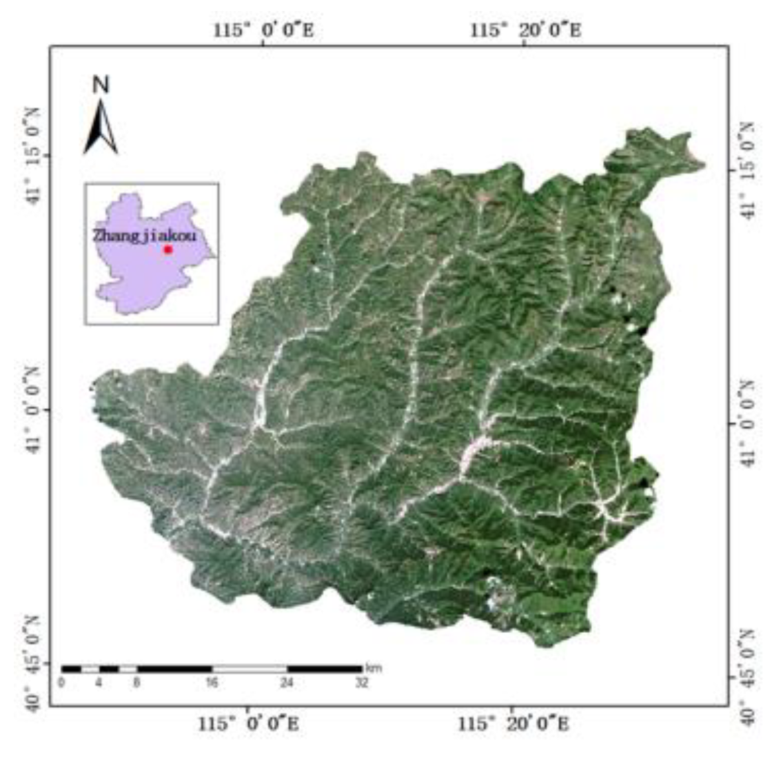
Figure 2.
DEM distribution of Chongli District.
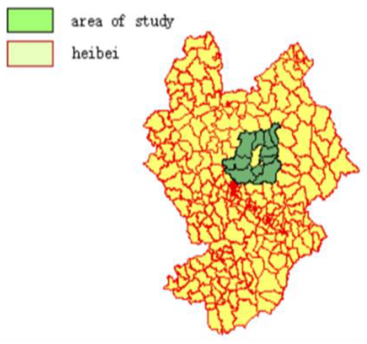
Figure 3.
DEM data processing (Grayscale images have been color processed).
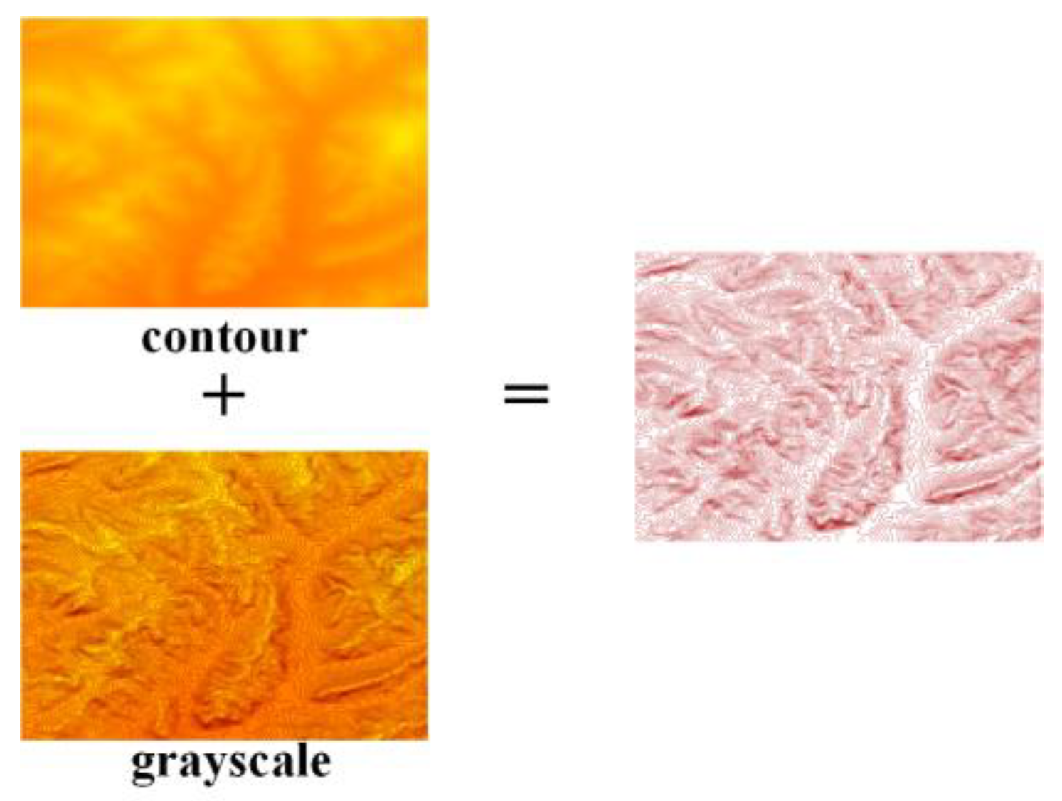
Figure 4.
Mountain sample.
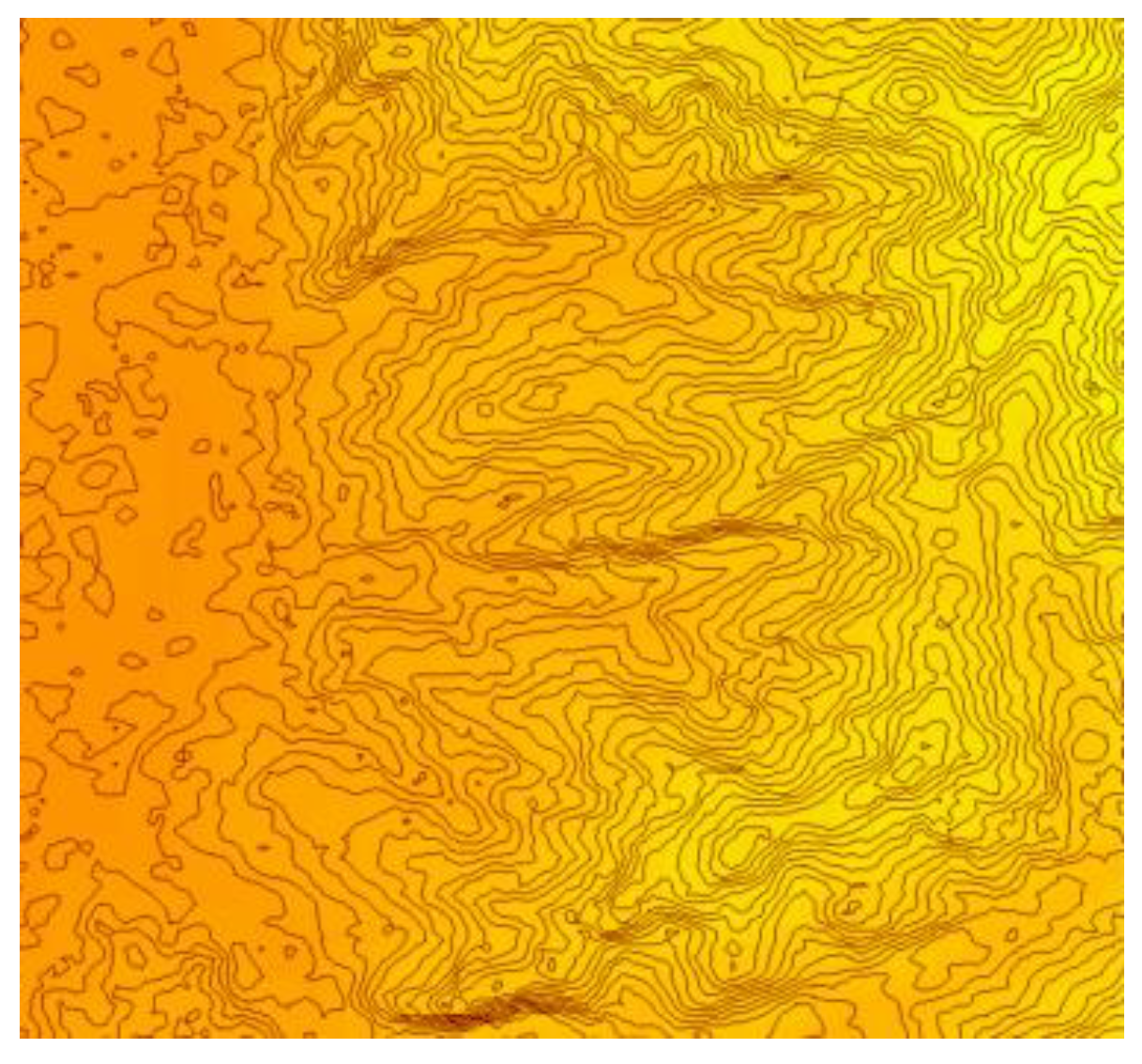
Figure 5.
DEM Zhongshan vertex diagram.
Figure 6.
Altitude distribution map of Chongli
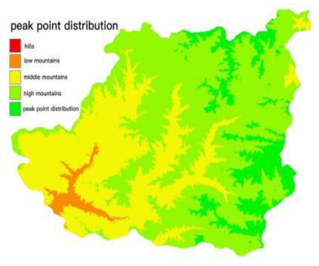
Figure 7.
Topographic relief diagram of Chongli.
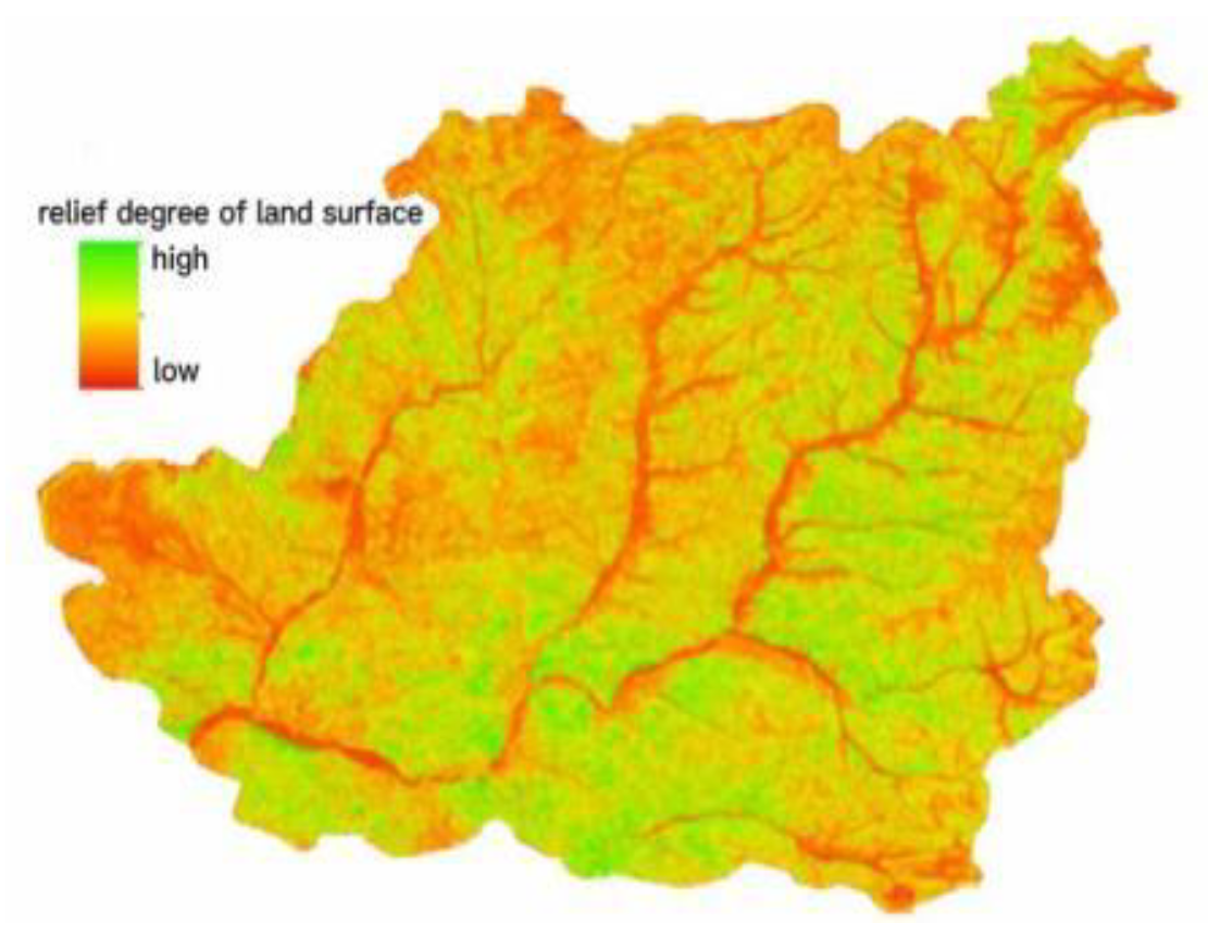
Figure 8.
Topographic map of Chongli District.
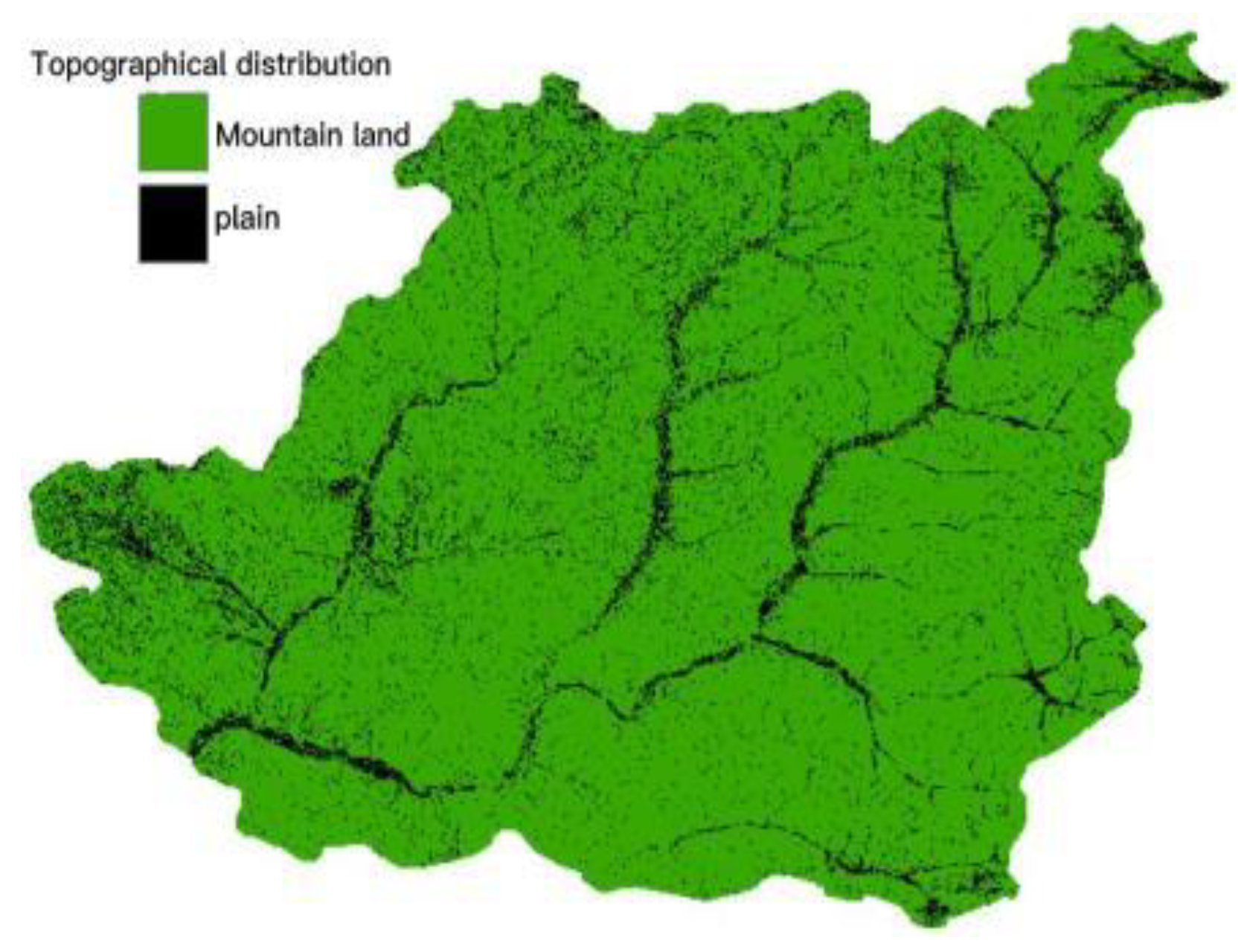
Figure 10.
Flow chart of water system identification in Chongli District.
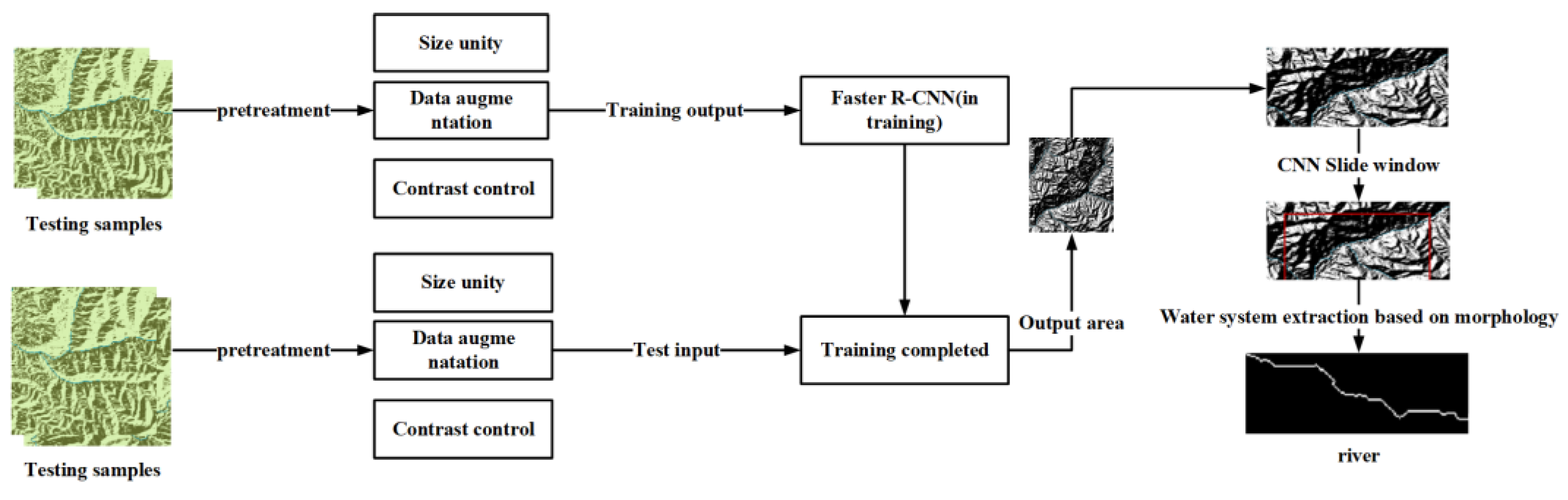
Figure 11.
Faster R-CNN algorithm flow chart.
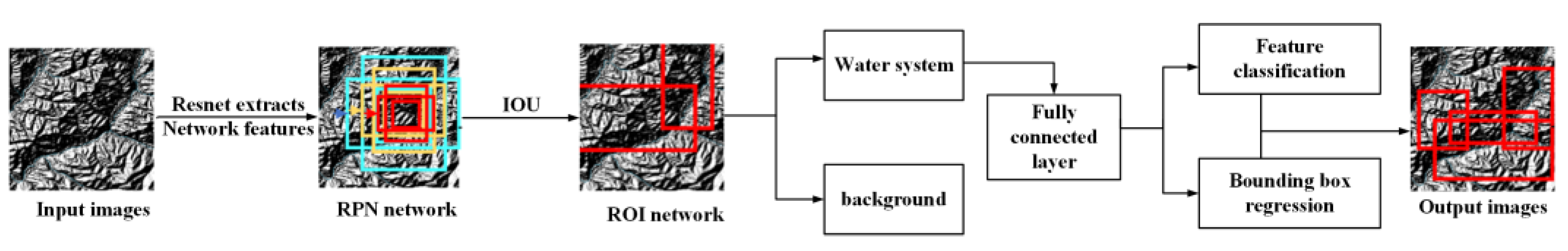
Figure 12.
RPN network.
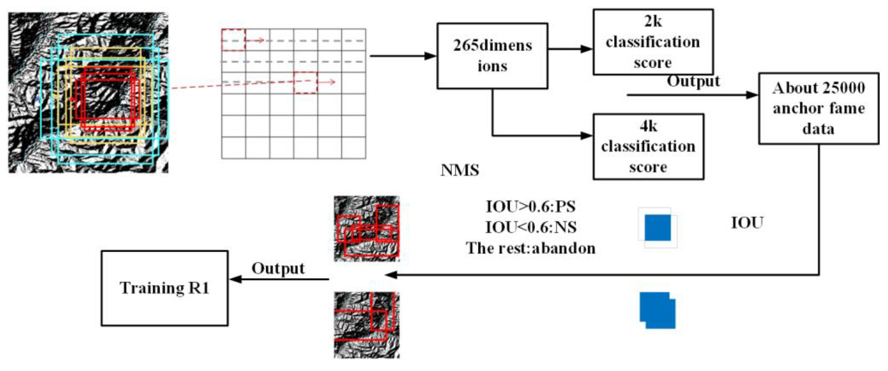
Figure 13.
CNN training steps.
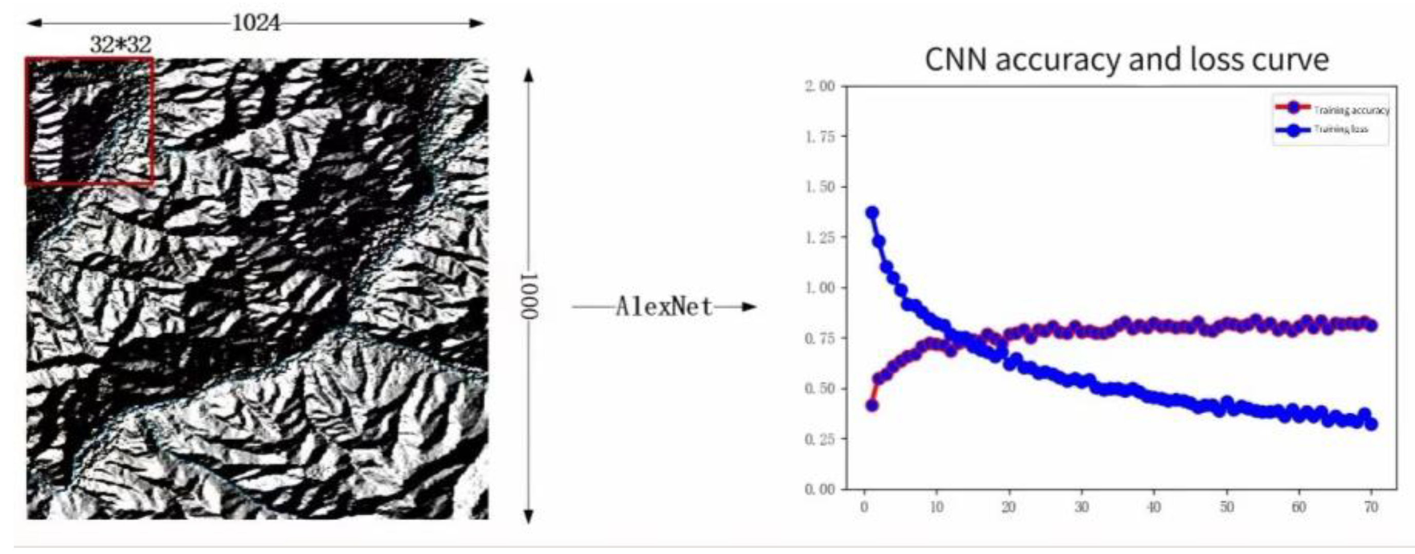
Figure 14.
AlexNet neural network model diagram.
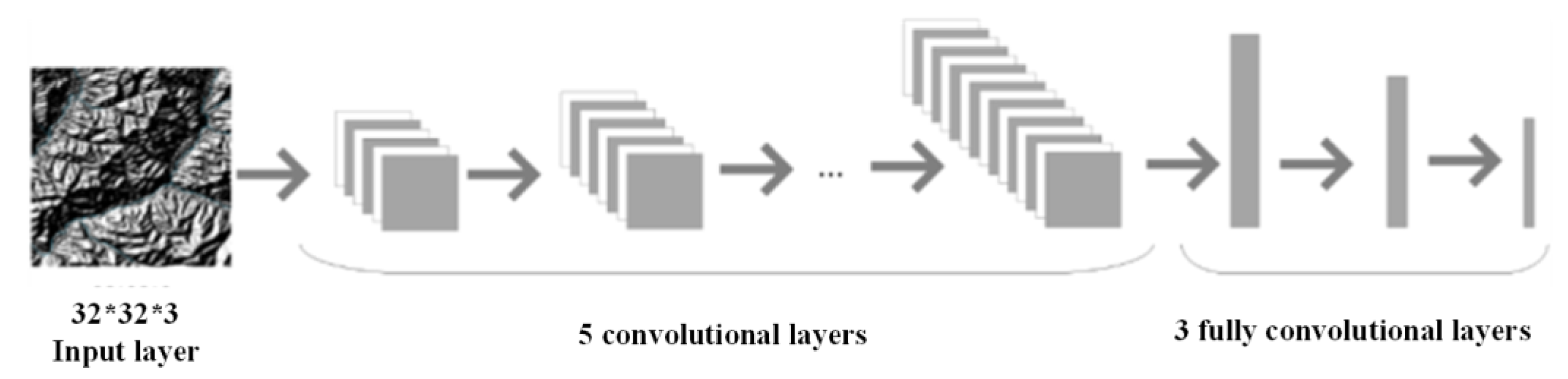
Figure 15.
AlexNet transfer learning.
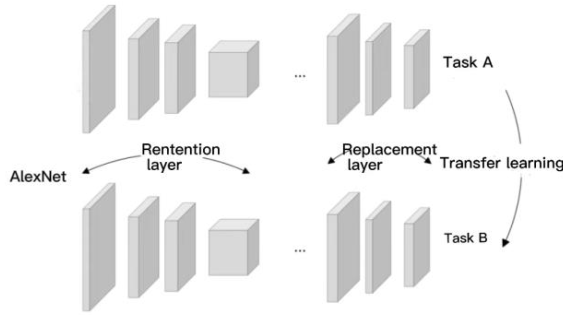
Figure 16.
Water system width comparison.
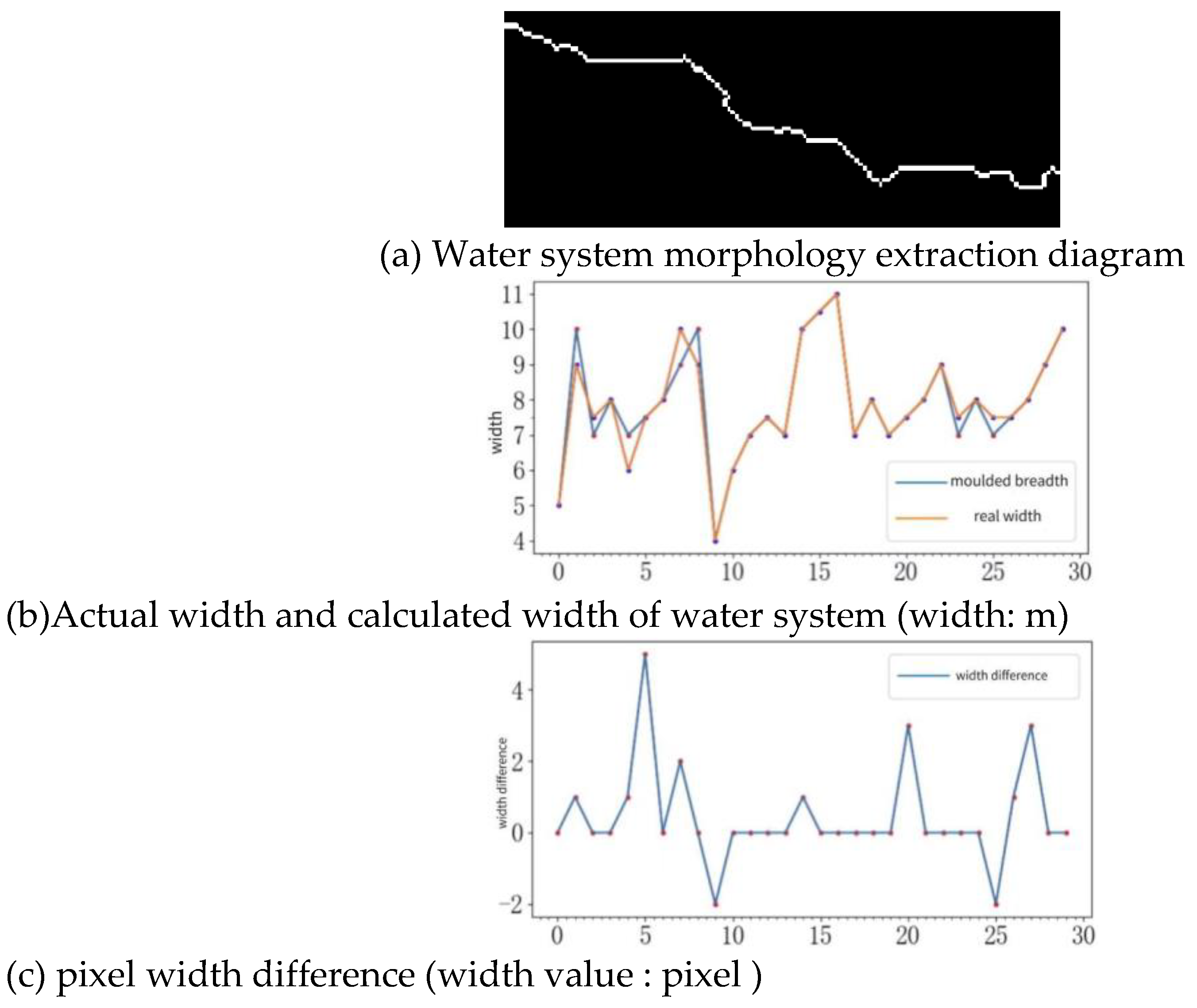
Figure 17.
Image annotation.
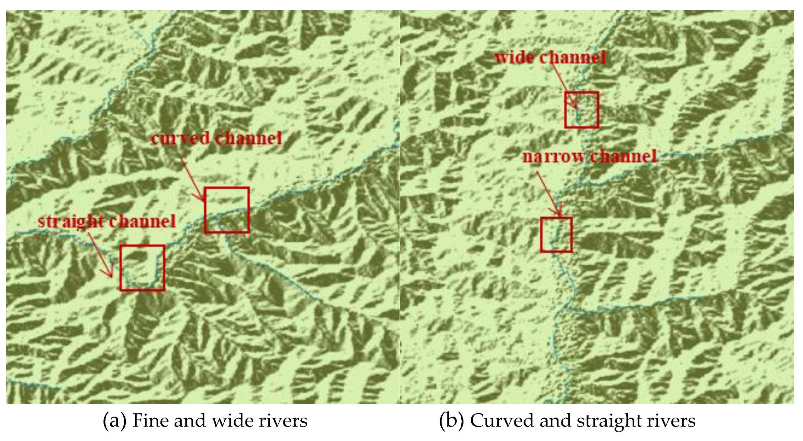
Figure 18.
Distribution map of peak points in Chongli District.
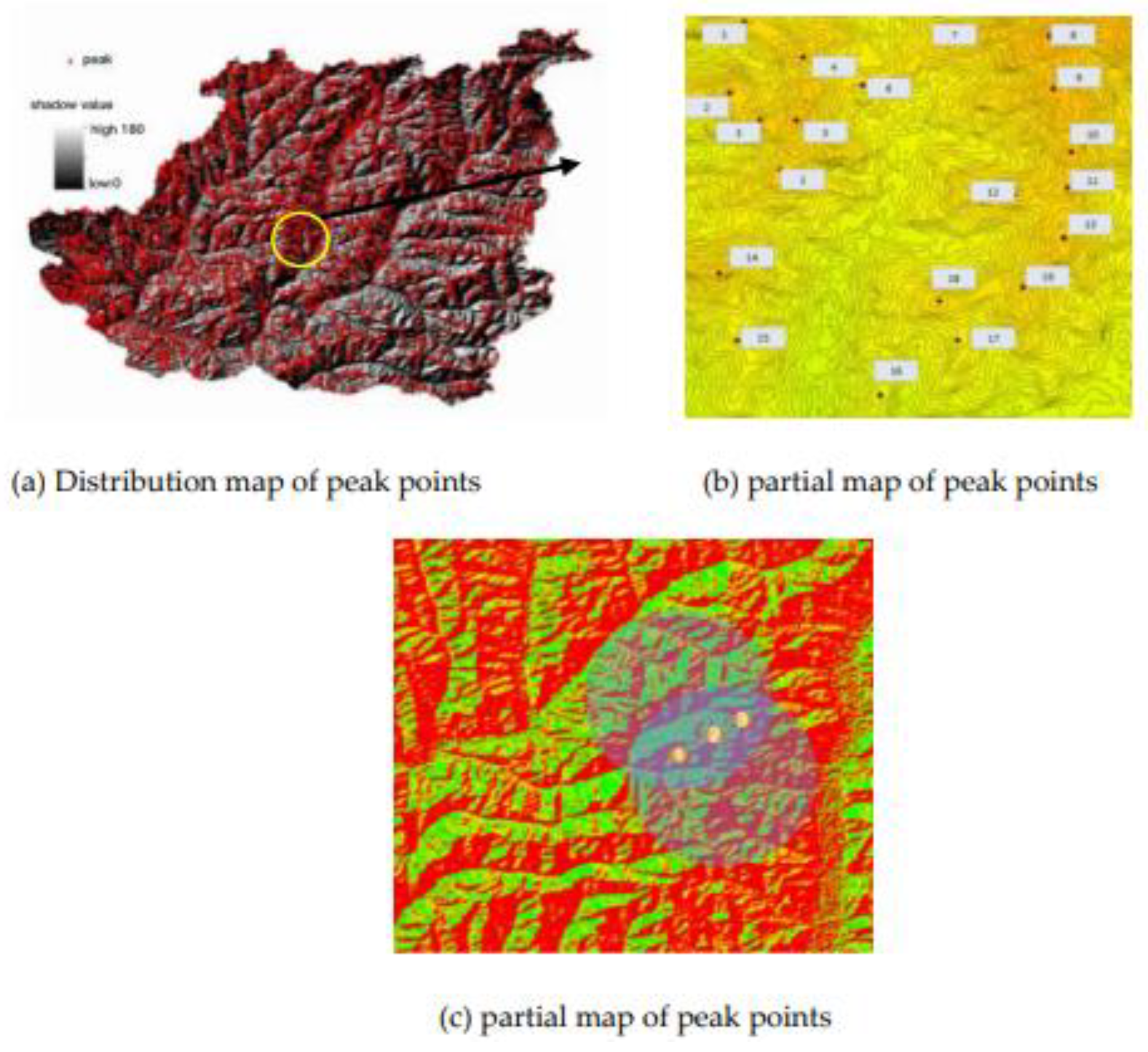
Figure 19.
K-Means preliminary classification results.
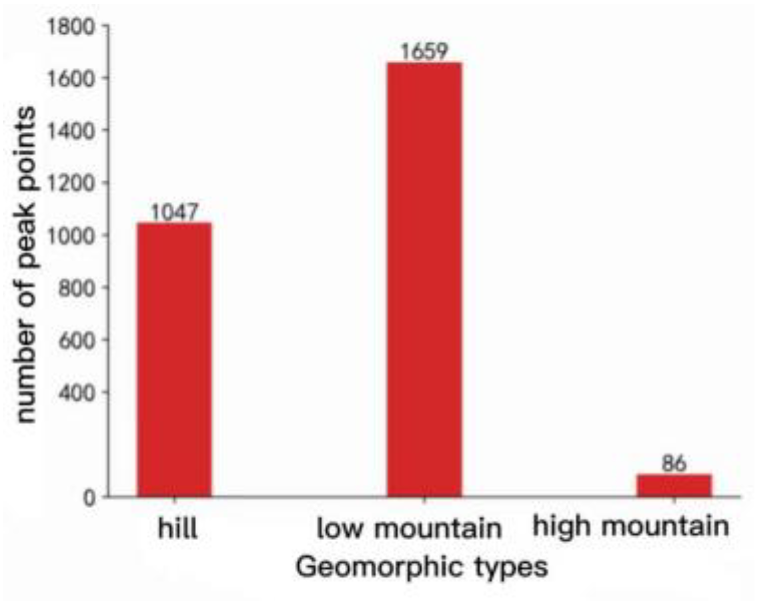
Figure 20.
K-Means preliminary classification results.
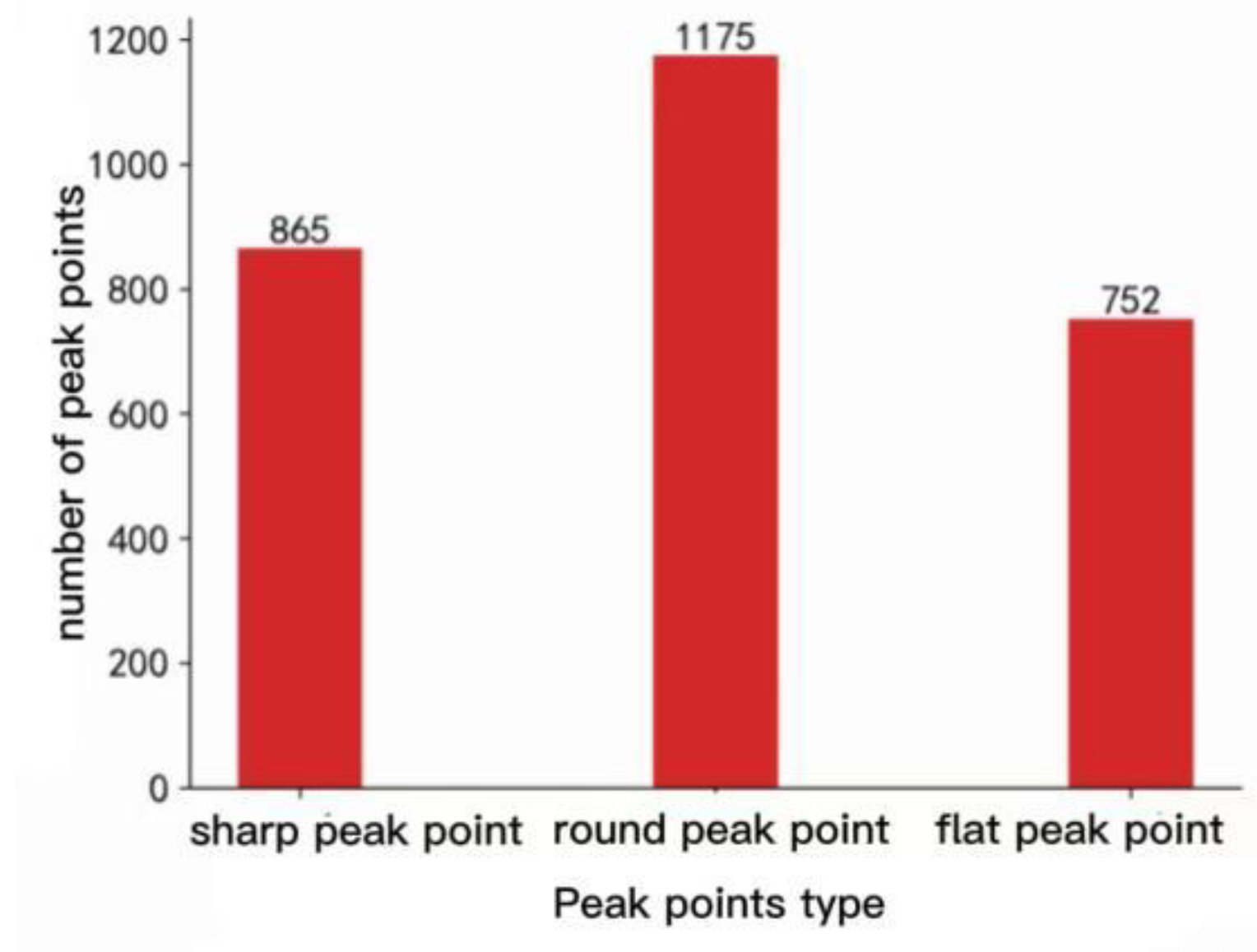
Figure 21.
Test results.
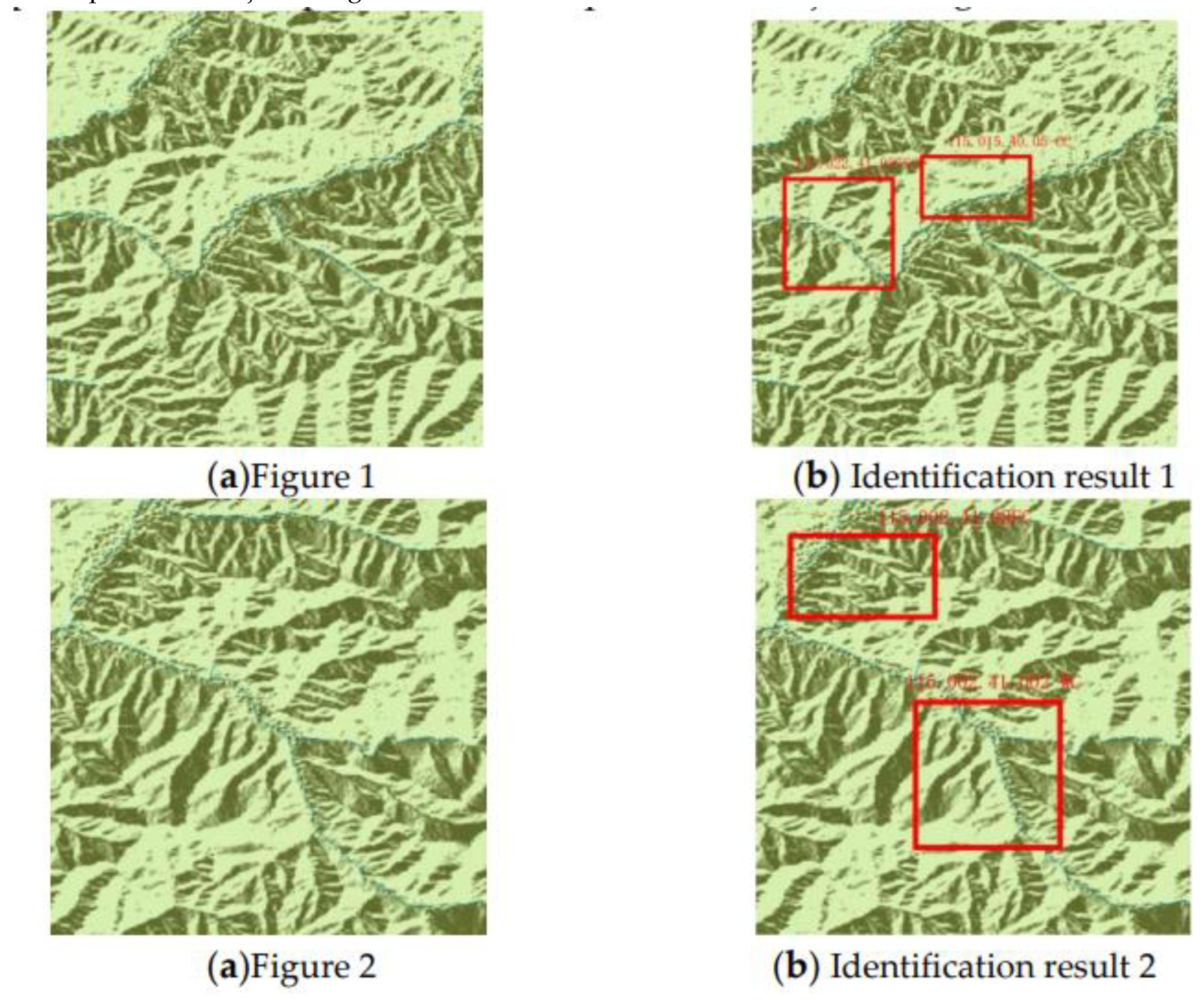
Figure 23.
Distribution map of peak points without geomorphic classification.
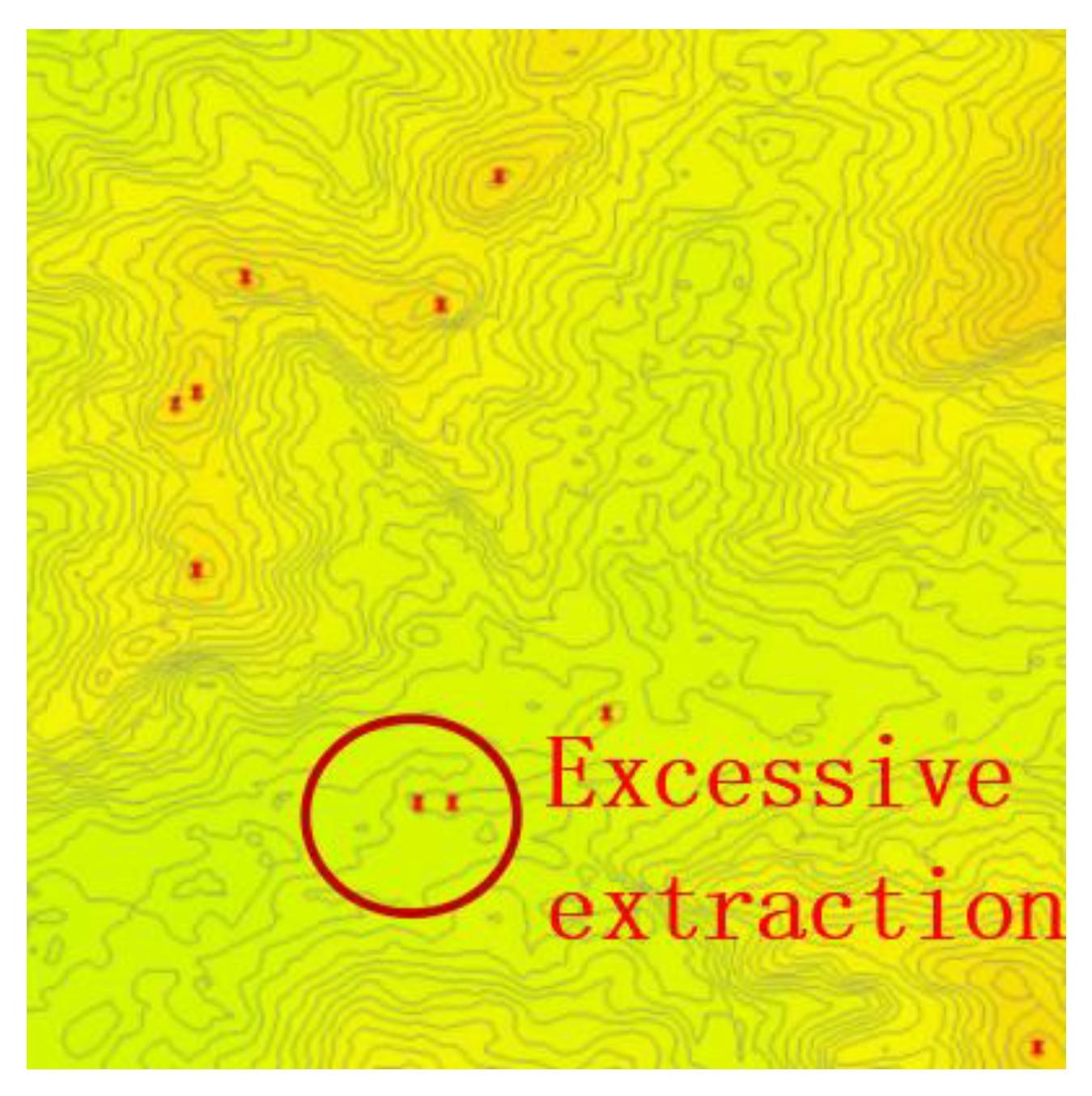
Figure 24.
Distribution map of peak points.
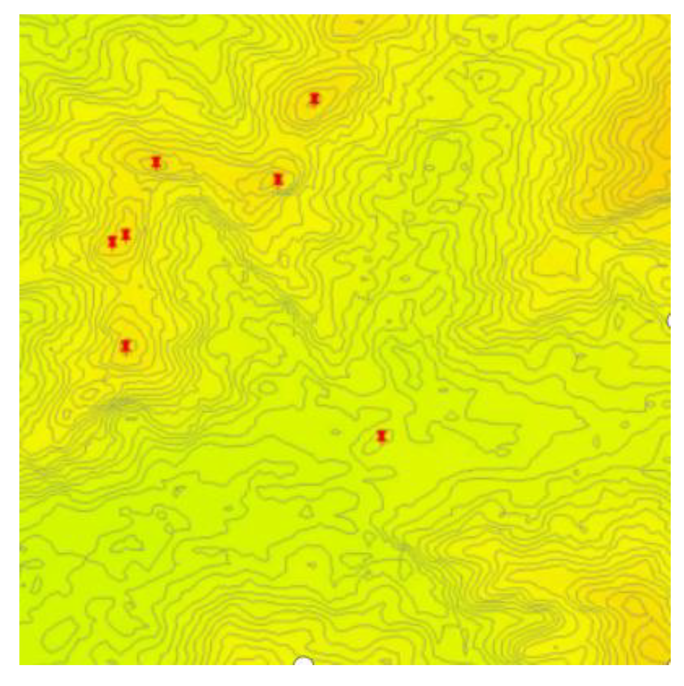
Figure 25.
Recognition results of mountain vertices under different conditions.
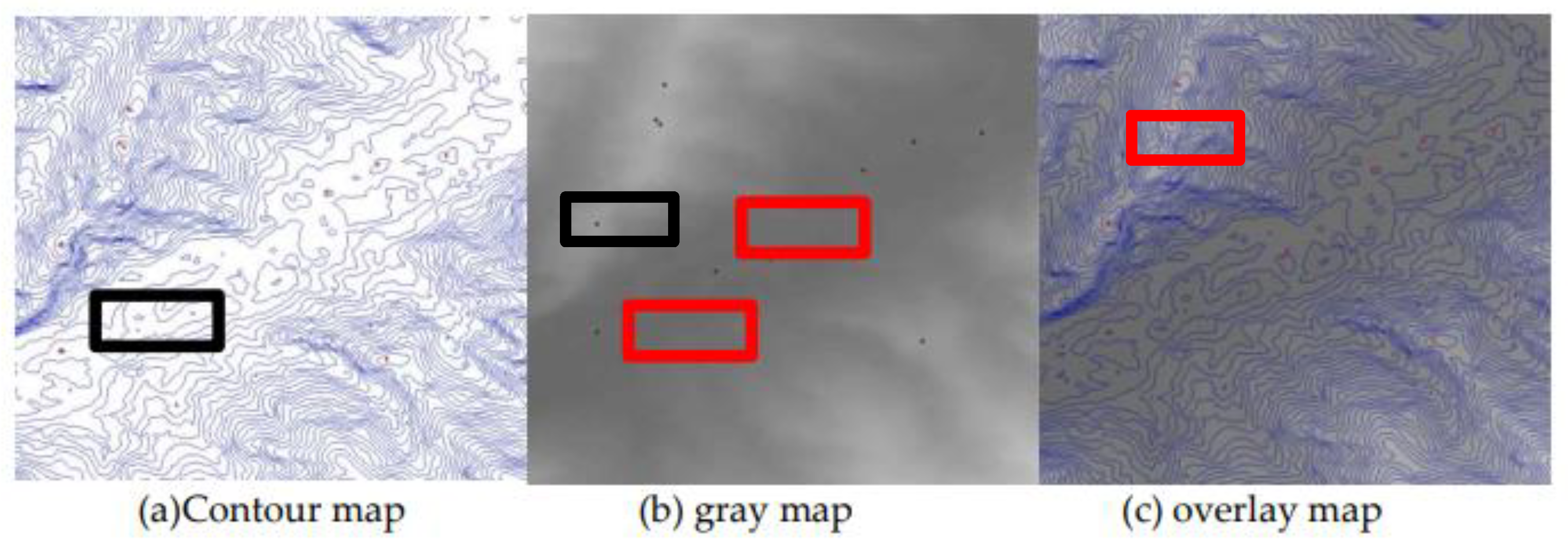

Table 1.
Peak sample data.
| label | ||||
|---|---|---|---|---|
| 370 | 120 | 430 | 200 | 1 |
| 325 | 240 | 370 | 370 | 1 |
| 300 | 425 | 250 | 440 | 1 |
Table 2.
Classification standard of basic geomorphic forms.
| Geomorphic type | hill | Low mountain | high mountain | Extreme mountain |
|---|---|---|---|---|
| Undulation(m) | 20-150 | >150 | 260-600 | >2000 |
| Altitude(m) | <500 | 500-800 | 2000-3000 | >5500 |
Table 3.
Geomorphic type and minimum reference elevation of mountain top.
| Geomorphic type | hill | Low mountain | middle mountain | high mountain | |||
|---|---|---|---|---|---|---|---|
| Average altitude(m) | <500 | 500-800 | 800-3000 | >3000 | |||
| Undulation(m) | 20-150 | <150 | ≥150 | <200 | ≥200 | <500 | ≥500 |
| Minimum elevation of peak(m) | +30 | +30 | +200 | +200 | +500 | +500 | +1000 |
Table 4.
True false positive mixed matrix.
| Predictive value | Authenticity | |
|---|---|---|
| positive | Negative | |
| Positive | 500 | 900 |
| TP | FP | |
| Negative | 0 | 700 |
| FN | TN | |
Table 5.
Identification results under different conditions.
| Result | Contour map | Contour map | overlay map |
|---|---|---|---|
| Ri (%) | 15.41 | 7.52 | 4.25 |
| Ro (%) | 12.05 | 9.23 | 4.15 |
Disclaimer/Publisher’s Note: The statements, opinions and data contained in all publications are solely those of the individual author(s) and contributor(s) and not of MDPI and/or the editor(s). MDPI and/or the editor(s) disclaim responsibility for any injury to people or property resulting from any ideas, methods, instructions or products referred to in the content. |
© 2024 by the authors. Licensee MDPI, Basel, Switzerland. This article is an open access article distributed under the terms and conditions of the Creative Commons Attribution (CC BY) license (http://creativecommons.org/licenses/by/4.0/).
Copyright: This open access article is published under a Creative Commons CC BY 4.0 license, which permit the free download, distribution, and reuse, provided that the author and preprint are cited in any reuse.


