
Submitted:
25 April 2025
Posted:
25 April 2025
You are already at the latest version
Abstract
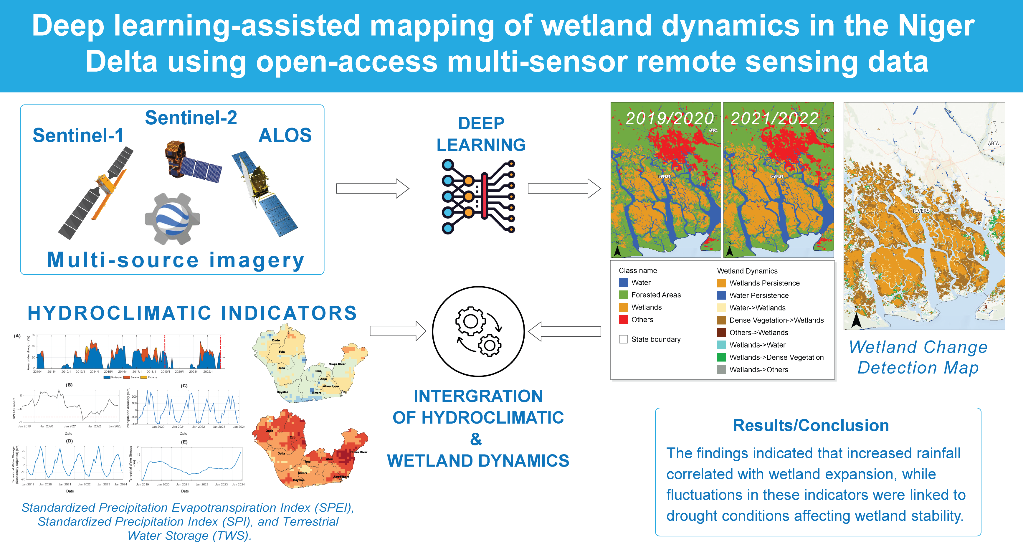
Wetlands play a crucial role in the global hydrological cycle and act as natural buffers that enhance resilience to extreme climatic events. However, they are increasingly being threatened due to human pressures. In this study, we assembled a deep learning (DL) framework to document recent changes in wetland dynamics in the Niger Delta using multi-temporal, multi-sensor satellite data. To achieve this, specific objectives were: (i) identifying optimal sensor combinations for wetland classification, (ii) evaluating DL model performance, (iii) performing land use/land cover (LULC) classification across two timeframes (2019/2020 and 2021/2022), and (iv) analyzing hydrological variability through satellite indicators and comparing with wetland changes. Several tests were undertaken to determine the best model for wetland mapping using the optimal multi-sensor image dataset as input in the DL models (Res-UNet and DeepLabV3). The results showed that the Res-UNet model, combined with the ResNet 152 backbone, outperformed the DeepLabV3 model (with identical backbones) in segmenting wetlands, achieving high F1 scores and overall accuracy (the F1 scores ranged from 0.83 to 0.91). Estimates of wetland transition across the landscape were obtained using the optimal DL model outputs as inputs for change detection analysis. The change detection analysis revealed that converting dense vegetation to wetlands was the main driver of wetland gain, while wetland loss primarily emanated from transitions to dense vegetation. The spatial extent of wetland loss was estimated to be 27,346 hectares, whereas gains totalled 98,453 hectares. Furthermore, the study established links between hydroclimatic indicators and changes in wetland, emphasizing the influence of climatic conditions and human activities on wetland expansion. Ultimately, our findings illustrate the potential of advanced remote sensing and deep learning for wetland monitoring and highlight the necessity of informed conservation strategies for fragile ecosystems.
Keywords:
wetlands
; deep learning
; Res-UNet
; DeepLabV3
; drought
; terrestrial water storage
; sentinel-1 &2
; change detection
1. Introduction
Wetlands play an irreplaceable role in maintaining the global hydrological cycle, making the protection of their ecosystem diversity a matter of great significance [1,2]. These globally threatened habitats are vital to climate change mitigation, biodiversity, and human health [3], contributing directly and indirectly to the total economic value of the planet [4]. From a biodiversity perspective, only one percent of the Earth’s surface is covered by freshwater wetlands, yet over 40 percent of the world’s species reside within them [5]. The Niger Delta region is part of this fragile wetland and terrestrial ecosystem, facing a diverse range of environmental challenges caused by anthropogenic factors such as agricultural degradation, oil and gas-related pollution, seismic activities, overexploitation of forest resources, rapid urbanization, and the illegal harvesting of trees for construction [6,7,8]. Therefore, policymakers, the government, and key stakeholders need access to information regarding the spatial and temporal dynamics associated with these endangered wetland habitats.
Landsat satellite data has been extensively used for wetland and general land use and landcover (LULC) inventories for change detection analysis, benefiting from its long-term records and broad coverage [9,10,11,12,13]. However, Landsat’s 30-meter spatial resolution limits its ability to capture smaller wetland areas, and frequent cloud cover in tropical regions like the Niger Delta hinders the acquisition of cloud-free imagery [14,15]. Issues such as inundation fluctuations, spectral similarity, and cloud pollution present unique challenges in wetland and LULC mapping in these areas [16]. Additionally, the 8–16-day temporal resolution of Landsat images restricts observation opportunities. Recent studies highlight the integration of finer spatial resolution 10-meter multi-sensor fusion, such as Sentinel-1 and Sentinel-2 satellite images, which offer more frequent revisit times (3-5 days) and increase the chances of acquiring cloud-free imagery [16,17,18,19]. Combining multi-temporal spaceborne multi-sensor data (including radar, optical, and elevation data) for large-scale land cover and biomass mapping emphasizes the effectiveness of this approach for habitat mapping. This integration of S1 and S2 imagery enhances wetland and LULC mapping by addressing limitations associated with single-use optical imagery and improving the overall quality and frequency of data collection [18,19]. The combination of Sentinel-1/2 time-series imagery and DEM data provides comprehensive datasets that improve the classification accuracy of different wetland types [20,21].
Several studies have explored the combined use of optical, radar, and topographic information to map wetlands and other LULC [22,23,24,25,26,27]. The RF-supervised machine-learning classifier has been employed in wetland and LULC mapping on national and regional scales [28,29,30]. Past studies have utilized RF feature importance selection to enhance LULC classification accuracy by combining S1 SAR, S2 optical, and DEM elevation data [20,31,32]. Considering the heterogeneous nature of wetlands in the Niger Delta [33] and the difficulties associated with spectral similarities, the role of feature selection is crucial in improving the performance of machine-learning approaches [34]. Hence, effective feature selection is essential for image classification. It optimizes the model’s computational efficiency by removing redundant variables from the modelling process while ensuring classification accuracy. Using cloud computing platforms such as GEE, DL models (such as DeepLabV3 and Res-UNet) can process large amounts of multi-source data, making this combination a scalable and efficient approach [20].
Deep learning models, such as convolutional neural networks (CNNs), have been effectively utilized to create accurate wetland and land use and land cover (LULC) map products [35,36,37,38,39,40,41,42,43,44,45,46]. CNNs can learn complex image patterns and often outperform shallow learning algorithms like random forests in remote sensing applications [21,39,47]. Studies have shown that integrating multi-temporal radar and optical data significantly enhances model performance [22,23,24,25,26,27]. For instance, modified U-Net models have outperformed other models in land cover classification tasks. Exploiting deep learning techniques like Res-UNet [21,40,41,44,46,47,48,49], CNN [35,37], and DeepLabV3 segmentation model [45,50] for LULC mapping has shown great promise. Although limited studies are focusing on deep learning techniques for wetland and LULC mapping in the Niger Delta due to limited ground training data and cloud-free imagery, the potential for managing these fragile ecosystems globally through multi-source satellite data analysis is immense.
Both surface and sub-surface water dynamics, including factors such as rainfall, river inflows, and groundwater, typically influence wetland hydrology [51,52]. In humid coastal regions, high rainfall and variations in drought intensity and frequency can significantly impact wetland water levels, leading to seasonal changes in inundation and spatial distribution. Dyring, et al. [53] explored the ecohydrological process in coastal groundwater-dependent ecosystems, such as wetlands, and how these are affected by climate change. Similarly, Tiner [54] evaluated the hydrology of wetlands with emphasis on the influence of tide, local weather conditions, and river discharge on wetland water levels. More concerns include rising temperatures and shifting precipitation patterns, further disturbing wetland hydrological balance. In the Niger Delta region, which is characterised by large lowland forest and highly productive freshwater swamps, the cumulative effects of human interference have heavily impacted wetland hydrology and distribution [55,56]. With advancements in hydrological monitoring, such as remote sensing and ground-based measurements, access to essential data for understanding these water cycles and assessing the effects of natural and anthropogenic changes on wetland ecosystems is now possible. By exploring the use of satellite-based water budget indicators (such as evapotranspiration, precipitation, drought conditions and terrestrial water storage), it’s possible to evaluate the relationship between wetland dynamics and hydrology. There are limited studies that have investigated this component of the study for the Niger Delta region.
The overall aim of the study is to enhance the mapping of wetland changes in the Niger Delta using multi-temporal and multi-senor data as inputs in shallow and deep learning models developed for the region. Additionally, a critical connection between hydrological variability and the productivity of wetlands (in terms of their distribution in time and space) was established using satellite-based climatic indicators. The following are the four main objectives:
- evaluate the optimal combination of Sentinel 1 radar, Sentinel 2 optical, and topographic variables most suitable for wetland classification in the study area.
- develop a workflow that utilizes the optimal multi-sensor combination as input to evaluate the performance of two deep learning models (Res-UNet and DeepLabV3) and a random forest classifier.
- use the optimal model identified in objective (ii) to perform a LULC classification of two time periods (2019/2020 and 2021/2022) and a change detection analysis to understand the wetland dynamics across the study area.
- perform an integrated analysis using satellite-based water budget indicators (such as evapotranspiration, precipitation, drought conditions, and water storage) to understand better the region’s hydroclimatic variability and its relationship with wetland change in the Niger Delta region.
2. Materials and Methods
2.1. Study Site
The Niger Delta is situated in the southwestern part of Nigeria. It comprises nine states: Ondo, Edo, Delta, Bayelsa, Rivers, Imo, Abia, Akwa Ibom, and Cross River (Figure 1). Geographically, the region is bounded between longitudes 7° 45′ 0.9” and 9° 28′ 2.79” and latitudes 4° 16′ 23” and 4° 22′ 34”. The Niger Delta, like the rest of the country, has two alternating dry (January to March) and wet (April to September) seasons. The region’s average annual rainfall is between 2000 and 4021 millimetres [57], with the peak of the wet season occurring between June and September and dryer months starting in August every year. The main dry season begins in December and lasts until March. The temperature in the region remains relatively constant throughout the year, with an average temperature of approximately 27°C and minimal seasonal variation. Due to the proximity to the Atlantic Ocean, the Niger Delta region is characterized by high surface humidity (estimated to fall below 75%) and increases further inland [28,58].
The region is dominated by lowland rainforest, freshwater swamps, mangrove forest, salt marsh, and tidal mudflats along the shorelines [7,28] and is known to have a diverse range of flora and fauna, including rare species in critical habitats [7,55]. However, high levels of environmental pollution resulting from oil and gas-related activities, high pressures from urbanization and industrialization, uncontrolled farming practices, and industrial activities (such as mining) have resulted in devastating environmental problems such as wetland degradation and deforestation [9,55,59,60].
2.2. Inventory of Satellite Data Explored for Wetland Mapping
Due to the challenges associated with acquiring cloud-free optical imagery over the Niger Delta region, a multi-temporal and multi-sensor approach was adopted in this study. For the optical satellite images, only image scenes captured during the dry season (January to March) over multiple years were used in the analysis to avoid issues with cloud coverage. To ensure consistency was maintained for the radar datasets sourced from the S1 SAR sensors, a similar time frame was adopted for both the dry season and the radar data acquired in the wet season (i.e., the primary wet months and the late wet months).
In addition to the Sentinel satellite SAR and optical imagery, the Advanced Land Observing Satellite (ALOS) Digital Elevation (DEM) model covering the Niger Delta region was sourced from the GEE cloud computing platform. This section of the paper provides details of the satellite images used in the study. Appendix S.1 in the Supplementary Information presents the GEE codes for the Sentinel-1 and -2 image collection and global precipitation data used in the study.
2.2.1. Sentinel-2 Multispectral Imagery
All the S2 imagery used for this study was sourced from the GEE cloud-computing platform and within the same time frame as the S1 imagery. The time intervals adopted for the study captured the dry season months (January to March), the start of the wet season months (April to July), and the end of the wet season months (September to November). However, due to dense cloud cover during the wet months due to heavy rains, the S2 images used for the study were those captured during the dry months for 2019–2020 (later referred to as 2019/20) and 2020–2021 (later referred to as 2020/21). The S2 image collection was filtered using cloud scenes with a “cloudy pixel percentage” threshold of 40%. Furthermore, the GEE platform incorporated a function for cloud masking and indices calculation into the code. All the S2 bands needed to generate the optical indices were reduced using the median reducer function available on the GEE platform. As part of the GEE code, a function to calculate all the S2 optical indices evaluated in this study was included (see Table 1).
The NDVI [61] is a widely used vegetation health indicator and has been used in numerous wetland mapping studies. The combination of optical indices (such as NDVI and NDWI), the NIR, and SWIR bands are some standard input variables that have been shown to be valuable in land cover and wetland classification studies [62]. The SAVI, developed by Huete [63], accounts for the differential between red and NIR extinction through the vegetation canopy. It’s known to minimize the effects of soil brightness, making it a valuable input variable for wetland mapping. The CMRI utilizes information in the red, green, and NIR bands of the Sentinel-2 optical datasets. This optical index incorporates outputs from NDVI and NDWI indices to discriminate mangrove vegetation from non-mangrove by utilizing information related to greenness and water content (succulence) [64,65].
2.2.2. Sentinel-1 SAR Imagery
The S1 satellite SAR data used for the study were ground-range detected imagery captured in the vertical-horizontal (VH) and vertical-vertical (VV) dual-polarimetric Wide Swath mode. The study explored all available VV and VH dual-polarization channels acquired in the ascending and descending modes that overlapped the study area. These S1 images were sourced from the GEE cloud repository. The SAR images available on GEE were pre-processed using the Sentinel-1 Toolbox, which included steps such as thermal noise removal, radiometric calibration, and terrain correction. For this study, the S1 data were captured during the dry season months (January to March), the start of the wet season months (April to July), and the end of the wet season months (September to November) in 2019/20 and 2021/22. This was necessary to generate false-colour composites that would be used for visual interpretation and as inputs for the modelling component.
This study explored several S1 SAR-derived indices, including the seasonal normalized difference, ratio indices, and seasonal differences of selected SAR variables. Table 1 describes the S1 channels explored and the calculated indices.
2.2.3. ALOS DSM Elevation Data
For this study, the ALOS World 3D–30 m (AW3D30) asset available on the GEE cloud-computing platform was used as the source of topographic elevation data. The elevation dataset has a horizontal resolution of 30 metres and is based on the DSM dataset (5-meter mesh version) of the World 3D Topographic Data [66,67,68,69,70].
To ensure the ALOS DEM was usable, the 30-meter dataset was resampled to 10 metres using a bicubic interpolation technique to ensure proper grid overlap with the S1 and S2 imagery. Subsequently, the resampled grid was used to calculate the topographic wetness index (TWI). The TWI is a reliable proxy for relative soil moisture and shows levels of water accumulation in the earth’s topography [71]. Table 1 shows the equation for calculating the TWI.
2.2.4. Standardized Precipitation Evapotranspiration Index
The areas under drought were identified based on the 12-month cumulated time series of standardized precipitation evapotranspiration index (SPEI) data [72], which is publicly available (https://spei.csic.es/database.html). The SPEI is a multi-scalar biophysical indicator incorporating land surface conditions (e.g., evapotranspiration), providing a framework for understanding drought impacts and their cascading effects on hydrological systems [73]. The 12-month accumulation period was chosen for this study because it allows for capturing the impacts of drought on hydrological stores (e.g., soil moisture) and wetlands. Given that the Niger Delta region is typically wet, we define drought conditions as occurring when the drought index is consistently negative and reaches a value of -0.8. This threshold supports the characterization of hydrological drought, where decreased precipitation affects wetland productivity and was similar to the approach used in Cumbie-Ward and Boyles [74]. For this study, the different drought categories used for the SPEI and the Standardized Precipitation Index (SPI), later discussed in this section, were based on a modified version of the U.S. Drought Monitor (USDM) [75], which was more representative of local drought conditions in the Niger Delta. Table 2 presents the drought classification categories used in the study.
2.2.5. Terrestrial Water Storage
The change in terrestrial water storage (TWS) is the sum of soil moisture, surface water, groundwater, and canopy or wetland storage, based on gridded mascon monthly global water storage/height anomalies relative to a time-mean (RL06.1Mv03), derived from GRACE/GRACE-FO. These data are provided in a single netCDF file, with water storage/height anomalies expressed in equivalent water thickness units (cm). RL06.1Mv03 is an updated version of the previous Tellus JPL Mascon RL06Mv02. Further processing details can be found in Watkins, et al. [76] and Wiese, et al. [77].
2.2.6. Precipitation Data
The precipitation data is based on the Climate Hazards Center InfraRed Precipitation with Station data (CHIRPS) [78]. This dataset provides over 30 years of quasi-global rainfall data, combining 0.05° spatial resolution satellite imagery with in-situ station data to create gridded rainfall time series for trend analysis and seasonal drought monitoring. West Africa is one of the regions in the world where in-situ monitoring of rainfall and fluxes is limited. The CHIRPS data is a suitable and readily available rainfall product that enables the assessment of hydrological conditions in this region.
2.2.7. Standardized Precipitation Index
In addition to the SPEI drought a finer resolution product to visually understand the trends of drought severity was explored using the 12-month Standardized Precipitation Index (SPI-12), drought indicator. The SPI drought index developed by McKee, et al. [79] is widely used to assess metrological drought conditions. This drought index is versatile and capable of assessing precipitation-based measures for different timescale (short and long term) and has demonstrated to be an effective measure of metrological drought [80,81,82]. Short-term SPI is closely related to soil moisture, while the long-term SPI can be related to groundwater and reservoir storage.
Obtaining fine spatiotemporal and reliable precipitation data required to accurately detect extreme precipitation and drought conditions is necessary in studies like this Niger Delta based study. Based on similar techniques as adopted by Yu, et al. [83], we employed the use of the Global Precipitation Measurements (GPM) mission joint operated by the National Aeronautics Space Administration (NASA) and the Japan Aerospace Exploration Agency (JAXA) global precipitation dataset at high spatiotemporal resolution [84].
For this study, the GEE cloud-computing platform was used to source the GPM precipitation data. The GEE image collection (ee.ImageCollection(“NASA/GPM_L3/IMERG_V07”) with a date range of January 2001 to December 2022 was downloaded for the ND. Considering the ND is predominant covered by wetlands and tropical forest, all of which are heavily dependent on water no precipitation mask was employed in this study. The long-term time series GPM precipitation data was downloaded and subsequently used to generate the SPI-12 measure for the study area. In this study, the SPI-12 was calculated using the SPI library in R. The “spi” library in R was designed for calculating the SPI, which is a key tool for analyzing and assessing drought conditions over several time scales (e.g., 1–3 months and 12 months). The raw precipitation data was fitted to a gamma distribution and then transformed to a normal distribution. The SPI was obtained by converting the frequencies of precipitation records into quantiles that correspond to the standard normal distribution as demonstrated by Yu, Leng and Python [83]. In this study, a 12-month timescale was adopted and used to generate yearly mean and quarterly plots for the study area from 2019 to 2022. The quarterly maps (January to March, April to June, July to September, and October to December) were used to visualize the spatial patterns of average annual total precipitation. The Supplementary Information contains the link to the GEE for the GPM precipitation data used to calculate the SPI-12 measure.
2.3. Description of Classification Scheme
For this study, the land cover classification scheme used was in a similar format to the Food and Agriculture Organization’s (FAO’s) hierarchical Land Cover Classification System (LCCS) scheme [85] and similar studies [86,87]. The classification scheme employed in this study comprises the following classes: water, dense vegetation, wetlands, croplands, bare ground, and rangeland. Table 3 describes the land-use/land-cover (LULC) labels used in this study.
2.4. Remote Sensing Ancillary Datasets
A significant limitation of working in the Niger Delta region is the lack of access to reliable ground validation and training data. To address this challenge, open-access thematic layers, results from already published works focused on the region, existing global wetland products such as the global wetlands map product produced by the Sustainable Wetlands Adaptation and Mitigation Program [64], visual interpretation of available medium to high-resolution satellite imagery made available through platforms like Google Earth Pro, ESRI ArcPro basemaps, and false colour composites of the S1 and S2 images were explored. In addition to these open-access data sources, the ESRI-developed S2 10m Land Use/ Land Cover time series product was explored while developing a database of reference class labels used in building the shallow and deep learning models evaluated in this study (Karra et al., 2021; ESRI, 2022). This product was built using deep learning AI models and trained using billions of human-labelled image pixels [86,87,88]. Benhammou, Alcaraz-Segura, Guirado, Khaldi, Achchab, Herrera and Tabik [86] describe the data source explored for training the model and the methodology employed in generating the 10-meter S2 global land use/land cover product.
2.5. Methods
Figure 2 presents this study’s workflow for wetland mapping and change detection analysis. This workflow is outlined in five main steps, beginning with acquiring and preprocessing multi-source satellite data in Google Earth Engine (GEE). This cloud-based computing platform served as the source for already preprocessed and ready-to-use image collection for the S1 SAR, S2 optical, and DEM elevation data.
2.5.1. Extraction and Selection of Features for Modelling
The input features explored for the shallow and deep learning experiments were sourced from the multi-sensor information sources outlined in Figure 2 and Section 2.2 of this paper. These SAR, optical, and topographic features were inputs in a variable importance test using the RF classification algorithm. The RF model variable importance assigns scores for a feature’s contribution to the model’s performance. It entails calculating the mean decrease in impurity (MDI) and assigning higher scores to the most critical variables for making predictions and lower scores to the least important variables [89].
2.5.2. Building Class Labels for Eetland and LULC Modelling
The building of class labels used as input data for training, testing, and validating the developed shallow and deep learning models was based on the variability of land cover classes and the distribution of soil types across the study area. For this step, the harmonized world soil database version 2.0 (HWSD v2.0) [90] was employed for this study. The HWSD v2 dataset provides a global soil inventory that provides insights into soil properties such as their chemistry, morphology, and physical characteristics [91]. Figure 3 shows the HWSD layer used to determine the spatial distribution of the training and testing areas of interest used in developing the shallow and deep learning models for the Niger Delta region.
Based on these two criteria, sample areas of interest that met the required conditions were digitized as polygon extents and used to clip the ESRI-developed S2 10m LULC time series product. The clipped areas were used as input data for training, testing and validating the shallow and deep learning models evaluated in the study.
Using the defined sample outlines, based on the soil type and land-use criteria, stratified random sampling [92] was adopted to generate ground validation data for training the RF and DL models. Considering the challenges of getting accurate ground truth and validation data in the study area, selected areas (Figure 3) within the identified polygon extents defined using the soil properties served as a practical solution to selecting and generating the required ground validation points. Fig. S1 in the Supplementary Information presents the spatial distribution of training and validation data points used for the RF experiments performed in this study. Table 4 provides an inventory of the training labels for the RF models.
2.5.3. Hyperparameter Optimization for Developed Models
2.5.3.1. Random Forest Hyperparameter Optimization
This study used the cloud-based RF algorithm available on GEE to classify the multi-sensor image composite. The “Classifier” package on GEE handles supervised image classifications, including “RandomForest.” The hyperparameter optimization significantly improves the model’s performance. For this task, a subset of the optimal multi-sensor imagery, comprising 10 image layers (as described in Section 3.1, results of the variable importance test) for the 2019/20 time interval, was used as input for the hyperparameter optimization test of the RF model. The results of this test were applied to the 2021/22 multi-sensor image composite. The RF hyperparameters employed in this study are as follows:
- numberOfTrees: This parameter refers to the number of trees used in the RF model. Increasing the number of trees can significantly improve the classification accuracy of the RF model as it captures more patterns in the input data. However, this is computationally demanding, resulting in greater processing time. After performing the hyperparameter optimization tests, the number of trees for used for classifying the 2019/20 and 2021/22 optimal multi-source collection was 100. The evaluated number of trees used for the hyperparameter evaluation was 50, 100, and 200.
- variablesPerSplit: The variables per split parameter specifies the number of variables (or features) to consider at each split of the RF tree. By limiting the number of variables considered at each split, this parameter introduces some degree of randomness to the model. It increases the diversity among the trees, improving the RF model’s robustness and performance. The evaluated variables per split were 2, 5, and 10. Following the GridSearchCV scikit-learn hyperparameter test, the results indicated that 2 was the best variable per split for an optimal RF model performance.
- bagFraction: This parameter specifies the fraction of the input data to employ for each tree when sampling with replacements (i.e., bootstrapping). Employing a fraction of the data for each tree introduces a degree of randomness, which improves the RF model’s generalization level. It also reduces overfitting by ensuring each tree has access to different subsets of the data, resulting in a more robust model. For both RF classifications (2019/20 and 2021/22), the GEE bag fraction default value of 0.5 was used.
- minLeafPopulation: The “minLeafPopulation” parameter is used in decision tree-based classifiers like RF in the GEE cloud-computing platform. It specifies the minimum number of samples required at a leaf node and controls the smallest size of the terminal node in the tree. After several tests of the hyperparameters, the minimum leaf population variable was set to 1 to classify the 2019/20 and 2021/22 multi-sensor image composites. The multi-sensor image composite was based on input variables that were determined to be the most important in implementing the RF model, as identified through the variable importance test.
2.5.3.2. Res-UNet and DeepLabV3 models hyperparameter optimization
Hyperparameter optimization is crucial in training DL models for wetland and LULC segmentation. Yu and Zhu [93] provides a comprehensive review of hyperparameter optimization algorithms and applications to DL models such as DeepLabV3 and Res-UNet.
For this study, we explored using the same hyperparameters to allow for accurate comparison during the accuracy assessment of generated models. The hyperparameter optimization was based on the training data specific to each year considered in the study. The key hyperparameters considered for optimization are as follows:
Learning rates: The learning rate determines the step size at each iteration as the model moves towards a minimum of the loss function. It dictates the speed at which a deep learning (DL) model learns and is crucial for obtaining the best results. Table 5 outlines the minimum and maximum learning rates explored for the DL models implemented in this study.
- Batch sizes: The batch size refers to the number of training samples used in one iteration of the DL model. For this study, the number of image tiles processed in each model interface step can be described. The batch size adopted for all the DL models generated in this study was 8.
- Number of epochs: A value of 20 was selected and applied to all the generated models for this study. Considering the complexity and size of the multi-source data, a larger number of epochs would be recommended for future applications. This conservative value was selected to manage the computational power available during the study’s implementation. The model’s performance was evaluated on a validation dataset comprising approximately 10% of the input chips and labels used for training the DL model.
- Data augmentation parameters: These parameters refer to techniques for enhancing the input data required to train the DL model. Techniques such as rotation, scaling, overlapping, and flipping are used to artificially expand the volume of training data artificially, thereby improving model generalization. The training data are generated using the input multi-sensor image dataset and class labels representing the target landcover classes to be predicted. The tile sizes are the dimensions of the image chips generated during the extraction of training data for prediction. The tile sizes adopted in this study were 256 x 256 pixels (i.e., 2560m x 2560m). The padding, which represents the number of pixels at the image’s border from which predictions are blended for adjacent tiles, was set to 64. This approach reduces artifacts at the edges and smoothens the generated output. For all the DL models evaluated, the “predict background” and “test time augmentation” parameters were specified as false. The “predict background” parameter was set to false. It specifies whether the background class was classified during prediction. The final criterion, test time augmentation, was set to false for all the DL experiments conducted in this study. When test time augmentation is set to true, it merges the predictions of rotated or flipped variants of the input images into the final output.
- Backbone selection: The selection and fine-tuning of backbone architecture are crucial in DL modelling as they impact the model’s overall performance. The selection of a suitable backbone depends on the complexity of the input data, computational needs, and required performance. For this study, the ResNet backbone was selected. The Res-UNet and DeepLabV3 models combined with ResNet-34, -50, and -152 architectures were evaluated. The validation loss monitor metric was set to validation loss for all the DL experiments. When the validation loss does not change significantly, the model stops. Figs. S4 and S5 show the training and validation loss graphs for the DL models evaluated in the study (see Supplementary Information).
2.5.4. Wetland and LULC Classification and Segmentation
For this study, we evaluated the RF SL model and two deep learning (DL) segmentation models, the Res-UNet and DeepLabV3 models, which share a similar ResNet backbone. This section describes the SL and DL models evaluated in the study. This section of the manuscript focuses on the steps for building the RF classification model and developing the deep learning segmentation models, specifically the Res-UNet and DeepLabV3, which share similar backbone architectures (ResNet34, 50, and 152, respectively). This section of the paper outlines the modelling steps and parameters used, while Section 2.6.5 presents the accuracy metrics employed in the study.
2.5.4.1. Random Forest Machine Learning Model
The RF classifier model, a non-parametric “ensemble” model, was explored in this study to ascertain the best input variables to explore for landcover classification in the Niger Delta. It utilizes multiple decision trees (DT) in its classification process and is an effective tool for land cover classification studies. The RF algorithm classifies target features by constructing multiple bootstrapped and uncorrelated DTs. These DTs are singular bootstraps that split each node into the Gini criterion. In the context of remote sensing applications, the DTs with the majority vote are assigned a label [29,94]. The GEE RF classifier (‘ee.Classifier.smileRandomForest’) was used in this study to identify the input variables that perform best in the LULC classification and subsequent classification of the optimal multi-sensor variables. The RF-based variable importance was used to identify the multi-sensor variables that show potential or value in accurately classifying LULC. After several trials, the following parameters were selected for the RF classifier: 100 decision trees were used, and five variables were selected per split. A total of 3932 samples, with classes consistent for both years analyzed in the study, were employed for the RF classification, with 80% assigned to training and 20% to validation (Table 3, Fig. S1 in the Supplementary Information).
2.5.4.2. Res-UNet Deep Learning Model
The Res-UNet deep learning model is a 34-layer CNN pre-trained on the ImageNet dataset, which contains over 100,000 images across various classes designed for semantic segmentation of remotely sensed data. It merges the UNet architecture with residual connections, effectively capturing local and global features. The backbone of the Res-UNet comprises 33 convolutional layers, a 3 x 3 maximum pooling layer, an average pooling layer, and a fully connected layer [95]. The Res-UNet utilizes the UNet architecture as its backbone, featuring an encoder and decoder structure [96]. The residual connections mitigate the effects of vanishing gradient problems, allowing the model to learn more complex features, such as those found in multi-source image datasets. The Pyramid Scene Parsing Pooling technique captures contextual information at various scales, thereby enhancing the model’s ability to segment objects of different sizes.
2.5.4.3. DeepLabV3 Deep Learning Model
The DeepLabV3 DL is a fully conventional neural network (FCN) model for semantic segmentation. When used for semantic segmentation, a significant challenge of the FCN model is that the input features to the model become smaller as they pass through the network’s convolutional and pooling layers. This results in the loss of information on the input images and outputs, leading to low-resolution predictions and fuzzy object boundaries. To address this limitation, the DeepLab model utilizes the Atrous convolutions and Atrous Spatial Pyramid Pooling (ASPP) modules [97,98]. The architecture of the DeepLab model has since evolved, and the version used for this study was the DeepLabV3.
The architecture of the DeepLabV3 model comprises the following: feature extraction utilizing backbone networks such as ResNet, VGG, or DenseNet. For this study, the ResNet backbone was used. It employs the use of atrous convolution in a few blocks of the backbone to control the size of the feature map, an ASPP network to classify each pixel to their respective classes, and the passing of generated output of the ASPP network through a 1 x 1 convolution to obtain the size of the final segmented mask for the image. Several studies have explored the use of the DeepLabV3 DL model for classifying medium and high spatial resolution satellite imagery [45,46,50,99,100].
2.5.4.4. Deep Learning—Data Preparation and Segmentation Parameters
Preparing input data to develop and fine-tune the model is a crucial component of the deep learning (DL) workflow. Based on the RF variable importance test results, the optimal multi-sensor image dataset and training data were utilized to generate multiple image and label chips necessary for developing the ResU-Net and DeepLabV3 DL models. The training data used for both DL segmentation models were generated using the ArcGIS Pro geoprocessing tool named “Export Training data tool.” It’s well-known that deep learning (DL) models require large volumes of training data for predictions to accurately represent the mapped land use/land cover (LULC) classes. Hence, a more extensive spatial representation of the target landcover classes was generated for the DL modelling component (Fig. S2 and Fig. S3 in the Supplementary Information). Table S1 in the Supplementary Information presents a summary statistic of the exported training data analyzed in this study for DL models based on the two time periods examined (2019/20 and 2021/22, respectively).
This study employed the “Classify Pixels Using Deep Learning” geoprocessing tool in ArcGIS Pro to classify images. The classification parameters used for the DL models developed in this study included the batch size, padding, predicted background test time augmentation, and tile size. For this study, all the DL models evaluated had a batch size of 4 and tile sizes of 256 pixels. The batch size refers to the number of image tiles processed in each model interface step. The tile sizes are the dimensions of the image chips generated during the extraction of training data for prediction. Additional details of the DL parameters are provided in Section 2.6.4.2, which focuses on the hyperparameter optimization of the Res-UNet and DeepLabV3 DL models.
2.5.5. Accuracy Assessment of Wetland and LULC Predictions
The statistical measures used to evaluate the LULC products are a combination of the F1 score, overall accuracy (OA), producer’s accuracy (PA), and user’s accuracy (UA). The F1 score ranges from 0 to 1, with 0 representing the worst score and 1 representing the best. The F1-score is calculated using this formula: F1 = 2 * (precision * recall) / (precision + recall).
The OA, PA, and UA were calculated from the error matrices generated for each classified output (see equations 1 to 3 below).
For the DL semantic segmentation product accuracy assessment, the mean intersection over union (IoU) was used to calculate the accuracies of the study’s outputs. The mean IoU was based on the average of the individual class IoUs. The mean IoU gives users a better understanding of the segmentation performance and indicates overall accuracy (see equation 4).
where Xij = row in i column and j observations, Xi = marginal total of row I, Sd = total correctly classified pixels, n = a total number of validation pixels, TP = true positives, FP = false positives, and FN = false negatives.
In addition to evaluating the accuracy of the DL model outputs, the time taken to train and develop these models was critical. To test for differences in accuracy levels of generated products, the McNermar’s non-parametric test (z statistic) was applied to confusion matrices [101,102]. Equation 5 below shows how the z statistic is calculated:
where f12 and f21 represent the off-diagonal entries in the matrix. The difference in accuracy between a pair of classifications is considered significant at a 95% confidence level if the calculated z-score is more significant than 1.96 (positive or negative). Additionally, if the z-score is more significant than 2.58, it has a 99% confidence level.
2.5.6. Optimal Deep Learning Segmentation Versus Random Forest Prediction
To compare the performance of the optimal DL segmentation prediction and the RF prediction, an independent set of validation points was generated using an equal stratified random sampling approach [92,103,104]. Using the defined sample outlines, based on soil type and land-use criteria, an equal number of sample points were generated to represent distinct land cover classes across the study area. Considering the study’s focus is on wetlands, the seven-class generalized LULC products were reclassified into four classes: water, dense vegetation, wetland, and others (comprising the following grouped classes: croplands, developed area, bare ground, and rangeland). The validation points were ground locations with similar LULC over the two periods considered in this study. The information was sourced from the S2 false-colour composites for both periods (2019/2020 and 2021/2022), Google Earth, and high-resolution optical imagery obtained from ArcGIS Pro. For this study, 800 random sample points (200 per class) were generated each year and used for accuracy assessment. This approach ensures that a balanced representation of the seven classes was considered in the study. Fig. S7 in Supplementary Information illustrates the spatial distribution of sample points used to evaluate the accuracy of the RF and optimal DL segmentation products generated in this study.
2.5.7. Change Detection Analysis
To understand the recent changes in the spatial distribution of wetlands in the Niger Delta region, the four class wetland maps for each year were used as inputs for the change detection analysis with the “change detection wizard” tool in ESRI ArcGIS Pro software [105]. The geoprocessing tool enables the comparison of multiple raster layers captured at the exact location and at various times to identify the magnitude and type of change. This study employed categorical change to identify changes between the thematic grids (i.e., the optimal LULC prediction maps for 2019/20 and 2021/22).
2.5.8. Hydrological Indicator Trend Analysis
Hydrological conditions, including precipitation, water storage, and evapotranspiration, have been shown to play a critical role in shaping wetland habitats [106]. This study component aimed to gain a deeper understanding of the region’s recent climatic variability using satellite-based water budget indicators, including evapotranspiration, precipitation, and water storage. This study aims to gain a deeper understanding of the region’s recent climatic variability and investigate its relationship with wetland dynamics in the study area using spaceborne sensors. The existence of wetlands is typically linked to precipitation; therefore, utilizing the CHIRPS spaceborne sensor provides an indication of rainfall effects in the region. By combining the precipitation data with the SPEI drought index and TWS, complementary information on drought patterns can better inform the relationship between hydrology and spatial trends in wetlands across the study area. The timeframe of this investigation corresponded with the wetland change detection analysis (i.e., 2019 to 2022). Synthesis of wetland dynamics and hydrological conditions would provide a better understanding of wetlands’ spatial and hydrological dynamics in recent times. Monitoring wetland changes and hydrology significantly impacts management practices, as it enables better-informed decision-making through using hydrological indicator data (such as precipitation, evapotranspiration, and water budget) that inform managers’ decisions.
3. Results
3.1. Optimal Combination of Multi-Sensor Input Variables for LULC Classification
The optimal input variables for the LULC classification were selected based on the RF variable importance test results discussed in Section 2.6.1. The RF variable importance test evaluated the S1, S2, and ALOS DEM-derived variables described in Table 1. This test was performed using the 2019/20 multi-date and multi-source imagery.
The study explored a total of 28 multi-date and multi-sensor variables. Figure 4 shows the chart of the multi-sensor variables evaluated in this study (Table 1) for the data acquired in 2019/20. The multi-sensor variables classed as important by the variable importance test were: S2 SWIR bands (B11 and B12), ALOS DEM, SWI (S2 optical index), VVdry (S1 SAR channel), CMRI (S2 optical index), NDVI (S2 optical index), VVwet (S1 SAR channel), VHdry (S1 SAR channel), VHwet (S1 SAR channel), NDWI (S2 optical index), S2 red band (B4), SAVI (S2 optical index), GDVI (S2 optical index), S2 blue band (B2), and SAR indices (NIdry, NIwet, RIdry, and RIwet) (Figure 4). The least important multi-sensor variables for the RF model were excluded from subsequent analysis.
From the 22 outstanding multi-sensor input variables classed as necessary for the modelling process, those that provided duplicate or similar information to the model were excluded. For example, only one optical band in the SWIR region was selected for this study, specifically B11. NDVI and NDWI were dropped and replaced with CMRI because these input variables were used to generate the index. The visible and NIR bands (i.e., B3, B4, and B8) were excluded, as these served as inputs in some of the optical indices classed as significantly necessary in the RF model. The optical index excluded from further analysis was GDVI. Based on this criterion, a 10-band multi-sensor image composite consisting of the following input variables: CMRI, SAVI, SWI, EVI, B11, VVdry, VVwet, VHdry, VHwet, and ALOS DEM was identified as the optimal multi-sensor dataset for wetland and LULC mapping across the study area. This 10-band, multi-date, and multi-sensor dataset was used for RF classification, Res-UNet, and DeepLabV3 DL segmentations.
3.2. Comparison of Deep Learning Segmentation
The performance of the Res-UNet and DeepLabV3 DL segmentation predictions was based on the best combination of F-1 scores for all the classes, the mean F1 score, and IoU accuracy metrics. Figure 5 presents the per-class metrics results of the deep learning model simulations performed in the study. The Supplementary Information document presents additional information related to the F1 scores (see Table S3). The results show that the best-performing deep learning (DL) model for both years was the Res-UNet model, utilizing ResNet-152 and ResNet-50 backbones (later known as ResUNet152 and ResUNet50). The inter-class F-1 scores for all classes in the Res-UNet152 and Res-UNet50 models for both years (2019/20 and 2021/22) ranged from 0.4 to 0.95. For the 2019/2020 year, the ResUNet152 model F1-scores were as follows: wetland F1 score = 0.865, mean F1 = 0.831, and IoU = 0.908. The wetland F1 score, mean F1 and IoU measures for the 2021/2022 ResUNet152 model were 0.87, 0.764, and 0.886, respectively.
Figures S8 and S9 in the Supplementary Information present the Res-UNet and DeepLabV3 segmentation maps generated for both years in this study. The segmentation map products generated using the DeepLabV3 model exhibit high degrees of overgeneralization, particularly in classes such as croplands and water. In this study, the Res-UNet model has been demonstrated to outperform the DeepLabV3 model in handling complex multi-sensor datasets for wetland and general land-use/land-cover (LULC) prediction. Hence, for subsequent analysis, the optimal ResUNet152 model was selected as the optimal DL model for both years and a suitable candidate for change detection analysis.
3.3. Res-UNet Deep Learning Segmentation Versus Random Forest Prediction
The next component of the study was comparing the performance of the ResUNet152 models for both years with the RF predictions generated as part of this study. To accomplish this task, an independent set of validation sample points not utilized in developing the deep or shallow learning algorithms was used to assess the overall performance of the deep and shallow learning models (see Fig. S7 in the Supplementary Information). To evaluate overall performance, the overall accuracy, F-1 score for the wetland class, and McNemar’s test for significant differences were generated using the error matrix of the Res-UNet and RF models. The overall accuracy of the ResUNet152 models for both years outperformed the random forest predictions. For the 2019/2020 predictions, the ResUNet152 prediction was 96.8% compared to the RF 92.8%. Similarly, the ResUNet152 (97%) prediction outperformed the RF (88%) model for the 2021/2022 prediction. The results of McNemar’s test showed that the ResUNet152 models for both years were significantly higher than the RF predictions (p < 0.01, see Table 6). The error matrix used to calculate the accuracy measures is presented in Table S4 in the Supplementary Information. Figure 6 shows the optimal ResUNet152 DL segmentation maps used for the change detection analysis. Compared to the ResUNet152 segmentation maps, the shallow learning RF predictions (Fig. S10 in the Supplementary Information) had prominent salt-and-pepper noise effects and mixed pixels. Overall, the ResUNet model was better suited for wetland and general LULC mapping and mitigating salt-and-pepper noise effects.
3.4. Wetland Change Detection Analysis
Using the Res-UNet152 wetland maps for both years, a change detection analysis was conducted to understand the variations in wetland and surrounding non-wetland classes. Since this study focused on wetlands, a binary approach involving wetland and non-wetland classes was adopted to present and discuss the change detection analysis results in this section of the paper. In 2019/20 the spatial extent of wetlands in the ND was 277,445.72 hectares, while in 2021/22 it was recorded as 348,552.67 hectares (Figure 7). The change detection results showed that the spatial extent of unchanged wetland class from 2019/20 to 2021/22 was approximately 250,100 hectares (2.3% of the entire study area), while wetland loss and gain were 27,346.2 hectares (0.2% of the ND) and 98,453.1 hectares (0.9% of the ND), respectively (see Table 7). Table 7 illustrates the spatial changes of wetlands and non-wetland classes.
Figure 8 shows the proportion of wetland loss and gain from 2019/2020 to 2021/2022 in the Niger Delta. The dominant contributor of wetland loss in the ND over the time-interval analyzed was its conversion to dense vegetation totalling 22,965 hectares, 84% of the affected wetland (See Figure 8a). This was followed by wetlands transitioning to open water having an area of 3,854 hectares (14% of total wetland loss), and the least contributor being wetlands transitioning to other land uses (predominantly, croplands, developed areas, and fallow land) with an area of 527 hectares (2% of total wetland loss). For wetland gains, the results showed that the greatest contributor to wetland gain was attributed to dense vegetation being converted to wetland habitats (a total of 94,007 hectares, representing 95.5% of total wetland gain over the time analyzed (Figure 8b). The next significant contributor to wetland gains in the ND was water classes converted to wetlands with a spatial extent of 4,175 hectares totaling 4.2% of wetland gain between 2019/20 and 2021/22. Figure 9 and Figure 10 show the change detection map of the ND between 2019/2020 and 2021/2022 based on the optimal Res-UNet model predictions.
A mixture of natural and human-induced factors causes these transformations in the landscape across the ND. The impact of changes in hydrology, such as shifts in rainfall patterns, river overflows, or alterations in groundwater levels, can lead to saturated forested soils, which, over time, make these conditions suitable for wetland habitats. Other major human-induced drivers of forested area conversion to wetlands in the study area are deforestation, intensified felling of trees for agricultural purposes, over-exploitation of forest resources to logging activities, oil and gas exploration activities, and urban expansion [9,107,108]. In a study focused on community participation in forest management in the ND, Onojeghuo, Fonweban, Godstime and Onojeghuo [108] identified the several key drivers of deforestation in the region. These included subsistence agriculture, fuel wood harvesting, logging/timber extraction and intense commercial agricultural activities, overexploitation of forest resources, pressure from the high human population, and intensified levels of industrialization. Another significant contributor to the ND wetland transition is climate change’s impact. In the discussion section, the authors explore the connection between wetland dynamics and hydrological indicators, such as changes in precipitation, evapotranspiration, and water budget.
3.5. Hydroclimatic Indicator Trend Analysis
As indicated in Section 2.3, four hydrological indicators, namely the SPEI, TWS, SPI, and precipitation data, were employed to better understand the hydroclimatic conditions in the region and relate these proxies to changes in wetland over the period analyzed in this study. Typically, changes in hydroclimatic conditions are a consequence of climatic variability and human activities, which in turn can result in wetland degradation, loss of biodiversity and ecosystem services [109,110,111].
The TWS plays a significant role in better understanding changes in wetlands. Considering the dynamic nature of wetlands and reliance on water balance availability, the insights provided by TWS data show how these ecosystems are affected by natural and anthropogenic factors. The GRACE-derived TWS trend components result indicates a sharp rise in TWS between January 2019 and January 2020, with a peak that stabilized all through 2020 (Figure 11e). After this period, however, there was a gradual decline in TWS trend (January 2020-2021) and maintained a relatively steady low trend until mid-2023 (Figure 11e). In coastal West Africa, rainfall is the dominant driver of TWS [112], and any decline in TWS here reflects limited precipitation and below-average changes in surface and sub-surface water storage within the coastal wetlands. The slightly declining trend in TWS between 2019 and 2021 (Figure 11d and 11e) coincides with a pattern observed in the temporal variations for SPEI during the same period, with falling SPEI values starting in late 2019 and culminating in a dry or moderate drought event (Figure 11b). The amplitude of TWS in 2021 (Figure 11d) is one of the lowest and coincides with that of SPEI (Figure 11b). However, the lowest amplitude in rainfall anomalies observed in 2022 (Figure 11b) align with areas under drought in the same period (Figure 11a), but the annual amplitude of change in TWS was markedly higher in the same year. This disparity re-emphasizes the impact of hydrological memory and the region’s lag between rainfall and TWS, especially after a drought event as seen here.
The SPI drought index was used to illustrate the spatial patterns of drought events and wet extremes across the ND from 2019 to 2022. This was averaged over a quarter basis and the results are shown in Figure 12. Between 2019 and 2020, the mean SPI-12 values ranged from near normal to extremely wet conditions (Figure 12). This trend corresponded with the rise in TWS over the same period (Figure 11e) and positive trend in the SPEI-12, which showed mildly or moderately wet conditions (Figure 11b) across the ND. The SPEI area under drought chart (Figure 11a) shows that the study area experienced moderately wet conditions. However, between 2021 and 2022, the SPI-12 results indicate a general trend of mild to extreme drought conditions over the four quarters for the ND. This corresponds with the steady decline in TWS for the same period as shown in Figure 11e, negative trend in SPEI-12 values (Figure 11 b), and severe extreme conditions of areas under drought as indicated in Figure 11a.
Overall, the combination of all four hydroclimatic variables (namely, SPEI, SPI, TWS, and precipitation) explored in this study indicates a rise in wet conditions between 2019 and 2020 and a subsequent decline to moderate and extreme drought conditions between 2021 and 2022.
4. Discussion
4.1. Optimal Multi-Date and Multi-Sensor Image Data Used in the Study
Based on the results of the variable importance test implemented in the study, an optimal multi-date and multi-source imagery comprised of derivatives from the Sentinel-1/2 and ALOS DEM imagery was utilized for the SL and DL model implementation. The S1-SAR derivatives that proved the most important were the multi-date VV and VH dual polarization channels captured during the dry (January to March) and wet seasons (September to November) for both years (2019/20 and 2021/22) investigated. Sentinel-1 SAR backscatter signals provide critical information, such as surface roughness, vegetation structure and soil moisture, that can complement general LULC and wetland mapping [113,114]. The inclusion of multidate SAR imagery has been shown to improve classification accuracy within mixed-vegetation zones significantly [115]Leveraging the massive cloud-based computational power and rich repository of ready-to-use satellite image collections, such as the Sentinel satellite SAR and optical data, this study generated cloud-free S2 optical imagery over the dry seasons for the entire study area, combined with S1 SAR dual polarization channels captured over the dry and wet seasons. The use of optical-derived vegetation (such as CMRI, SAVI, SWI, and EVI) and the SWIR channel (B11) is a valuable proxies that improve classification accuracy within mixed landscapes comprised of wetlands. Tran, et al. [116] explored DL models incorporating multispectral indices for mangrove mapping from satellite data. The study investigated the use of 17 multispectral indices, including the CMRI, SAVI, SWI and EVI, combined with time-series VV and VH dual polarization channels, and 13 spectral bands as inputs in a U-Net model for mangrove mapping. In comparison to this study, we have explored the combined use of multi-date dual polarization VV and VH channels, S2 optical indices calculated for the dry months (considering challenges associated with cloud-affected imagery during the wet seasons in the ND), the S2 SWIR (B11) spectral band, and topographic information contained in the ALOS DEM imagery. These input datasets were selected based on the variable importance test performed as part of this study’s workflow to ascertain the optimal multi-date and multi-sensor dataset for subsequent use in the Res-UNet and DeepLabV3 DL and RF SL model development for wetland mapping performed in the study. Previous studies aimed at exploring the importance of specific spectral indices and spectral bands for wetland mapping concluded that the red edge, NIR, and SWIR bands exhibited high importance for mapping [117,118,119]. Hence, spectral indices generated using these spectral bands would, in turn, encapsulate the spectral attributes of the observed reflectance. Examples include the CMRI, SAVI, SWI, and EVI (see Table 1), which rely on several combinations of the green, red, NIR, red edge, and SWIR bands. The inclusion of optical spectral indices, SAR time series, and topographic elevation, as adopted in this study, has been demonstrated to significantly improve wetland and general LULC mapping when employed as inputs in DL models as compared to SL techniques (such as RF).
4.2. Relationship Between Wetland Change and Hydroclimatic Indicators
The change detection analysis showed that for wetlands, 2.3% (250,099.5 hectares) of the entire landscape had unchanged wetlands between 2019/2020 and 2021/2022. For wetland gain and loss, 0.9% (98,453.1 hectares) and 0.2% (27,346.2 hectares) of the entire landscape were disturbed simultaneously. The trend of wetland gains over the four years could be attributed to natural and human-driven factors. As demonstrated in this study, the changes in hydroclimatic conditions reveal a change in the precipitation levels, fluctuations in TWS and drought conditions over the four-year period. This change in climatic conditions can alter sea level rise and groundwater storage in the coastal wetland regions of the Niger Delta, resulting in the inundation of previously dense vegetation cover. In addition to climate change, the devastating effects of human-induced factors like deforestation, intensified agricultural practices, oil and gas-related activities, and mining activities have devastating effects on the dense vegetation classes (which comprises dense or tall swamps and mangroves with temporary water or a canopy that is too thick to detect water underneath, as well as wooded vegetation and plantations—see Table 2). The disturbance of forests and dense vegetation can disrupt the ecosystem and result in waterlogging or soil erosion, promoting wetland formation. Wetland habitats play a crucial role in the environment, serving as natural sponges to mitigate flooding, as a natural filter, and providing habitats for a vast range of plants and animals [120,121].
The impact of climate change is a prominent contributor to both wetland gain and loss [122,123]. For example, changes in precipitation and temperature can, in turn, lead to the rise or decline of water levels in wetlands, allowing vegetation to grow and transition into forested areas or reducing spatial coverage depending on the conditions. Other causes of wetland loss in the study area are anthropogenic factors resulting in land use changes such as reduced grazing or water management practices that, in turn, alter the dynamics of this fragile ecosystem, which in turn promotes forest growth. The fragile ecosystem of the ND makes it a unique and ecologically significant setting for investigating hydroclimatic indicators and wetland changes. Although this study has focused on recent wetland change over a 2-year epoch, we examined longer time-series hydroclimatic data (where available) and relevant results overlapping the timeframe of this study were assessed. The ND region faces significant environmental challenges that arise due to several factors, including climate variability, land use change, and anthropogenic factors such as intense urbanization, deforestation, and oil and gas exploration. These changes in LULC have resulted in high rates of forest loss, which are vital in supporting biodiversity and maintaining ecosystem balance [124]. This combined use of wetland dynamics information obtained from the change detection analysis results and interpretation of the hydroclimatic indicators evaluated in this study (namely, SPEI, SPI, TWS, and precipitation measurements) are an effective means of better understanding the transitional effects associated with wetland habitats in the ecologically fragile ND region. This approach provides better context as to the state of wetlands in the region and better informs decision-makers and policymakers on the next and best steps to conserving wetlands and other important ecosystems in the region.
4.3. Utilizing Long-Term Hydro-Climatic Conditions to Understand Wetland Trends
Our results also emphasize the composite role of changes in climatic conditions (e.g., rainfall) and human actions in driving significant land cover changes in a humid coastal region. The significantly more substantial rainfall and TWS amplitudes during the 2019/2020 period likely led to waterlogging of forested areas, creating favourable conditions for wetland expansion. In coastal regions, increased precipitation can saturate soil, reduce forest stability, and convert areas into wetlands. This is particularly pronounced in regions with poor drainage or already hydrologically connected to wetland systems. Subsequent moderate drought in 2022 highlights the vulnerability of wetlands to climatic variability and underscores the delicate balance between hydrology and human influence in shaping coastal ecosystems. The transition between dense vegetated areas and wetlands suggests that forests in this region are particularly vulnerable to hydrological and anthropogenic pressures. Wetland expansion at the expense of forests can indicate deforestation (natural or human-induced), where forest clearing accelerates soil saturation and enhances wetland formation during wet years. Deforestation and logging reduce evapotranspiration and increase surface runoff, promoting wetland conditions and can artificially increase water flow into low-lying areas. As demonstrated here, the combined use of water budget indicators like rainfall and GRACE-derived TWS supported by climate data (SPI and SPEI) provides a robust approach to enhancing understanding of water availability as an important driver of wetland dynamics, and human activities such as deforestation may have exacerbated changes in wetland during this period.
The combination of these water budget indicators, including GRACE, rainfall and evapotranspiration, provides an opportunity to understand climate change’s impact on the water balance and changes in the wetlands of humid regions like the Niger Delta. For instance, Penatti, et al. [125] demonstrated this using satellite data, including GRACE, to quantify Brazil’s hydrological dynamics of continuous wetland habitats. They evaluated a combination of several sources of water storage changes (sourced from GRACE), precipitation data (from the Tropical Rainfall Measuring Mission sensor), and evapotranspiration from the MODIS 16 sensor over 10 years. Results from their study demonstrated the value of estimating the hydrological regime and the entire basin’s internal variability based on the GRACE data. The change in TWS correlated well with precipitation, evapotranspiration and greenness over two to three-month intervals. Furthermore, the hydrological controls on surface vegetation changes across West Africa, analyzed using NDVI and supported by GRACE data, revealed distinct drivers in the region: while GRACE-derived TWS is a key driver in typically arid regions, rainfall predominantly influences vegetation dynamics in wetland areas, including the Niger Delta region [126]. Integrating advanced satellite geodetic methods, such as GRACE, with optical remote sensing approaches offers valuable insights into wetland hydrology and eco-hydrological processes [73]. This combination enhances our understanding of the connections between land cover transitions and climate change and how this translates to ecological impacts.
5. Conclusions
This study investigates the recent dynamics of wetlands in the Niger Delta using deep learning techniques and multi-temporal and multi-sensor satellite data. Wetlands are crucial for maintaining biodiversity and mitigating climate change. Yet, these invaluable habitats face significant threats from a mixture of changes in climate and anthropogenic activities such as pollution and urbanization. The focus of this study was to map the spatial distribution and dynamics of wetlands in the Niger Delta using multi-temporal and multi-senor data as inputs in shallow and deep learning models in the Niger Delta. The study outlines four key objectives: evaluating optimal sensor combinations for wetland classification, developing workflows for deep learning model performance assessment, conducting LULC classification for two time periods, and analyzing hydrological variability using satellite-based indicators.
The study identified a set of optimal input variables for LULC classification through the random forest variable importance tests. The results indicate that specific SAR (VVdry, VVwet, VHdry, and VHwet), optical bands and indices (CMRI, SAVI, SWI, EVI, and B11), and ALOS DEM significantly contribute to classification accuracy. The Res-UNet model, combined with the ResNet backbone, outperformed the DeepLabV3 model (with the same backbone) in segmenting wetlands, achieving high F1 scores and overall accuracy (wetland F1 score = 0.865, mean F1 = 0.831, and IoU = 0.908).
The change detection analysis results established that the spatial extent of mapped wetlands increased from 277,446 hectares in 2019/2020 to 348,553 hectares in 2021/2022. The spatial extent of wetland loss was estimated to be 27,346 hectares, while gains totalled 98,453 hectares. The change detection analysis revealed that dense vegetation conversion to wetlands was the primary driver of wetland gain, while wetland loss predominantly resulted from transitions to dense vegetation. Additionally, the study investigated the relationship between hydroclimatic indicators, such as SPEI, SPI, precipitation and terrestrial water storage (TWS), and wetland dynamics. The findings indicated a direct correlation between increased rainfall and wetland expansion, while fluctuations in SPEI, SPI, and TWS were linked to drought conditions affecting wetland stability.
Overall, this research underscores the importance of utilizing advanced remote sensing techniques, such as deep learning models, for effective wetland monitoring in the Niger Delta. These findings contribute to a better understanding of wetland dynamics and highlight the need for ongoing research to inform conservation strategies in fragile ecosystems. Policymakers and stakeholders must access accurate information about these ecosystems to inform conservation efforts.
Supplementary Materials
The following supporting information can be downloaded at the website of this paper posted on Preprints.org.
Author Contributions
Conceptualization, A.O.O.; methodology, A.O.O.; software, A.O.O., C.E.N, and A.R.O.; validation, A.O.O.; formal analysis, A.O.O., C.E.N, and A.R.O.; investigation, A.O.O.; resources, A.O.O.; data curation, A.O.O.; writing—original draft preparation, A.O.O.; writing—review and editing, A.O.O., C.E.N, and A.R.O.; visualization, A.O.O., C.E.N, and A.R.O.; supervision, A.O.O.; project administration, A.O.O.; funding acquisition, C.E.N. All authors have read and agreed to the published version of the manuscript.
Funding
This research received no external funding. Christopher Ndehedehe is supported by the Australian Research Council Discovery Early Career Researcher Award (DE230101327) for the project, Assessing the impacts of drought and water extraction on groundwater resources in Australia.
Data Availability Statement
Data will be made available on request. To visualize the change detection results and codes for the Google Earth Engine, an interactive mapping application was built using the Esri ArcGIS Experience Builder application. This can be accessed using this link: https://arcg.is/0mKLnv (accessed on April 20, 2025).
Acknowledgments
The authors would like to thank the anonymous reviewers and editors for their invaluable comments and input, which improved the quality of this manuscript. Also, thanks to Google Earth Engine and Copernicus for making free Sentinel and ALOS imagery available in the study. During the preparation of this work, the authors used Microsoft Copilot to improve grammar and sentence structure. After using this tool/service, the authors reviewed and edited the content as needed and take full responsibility for the content of the publication.
Conflicts of Interest
The authors declare no conflicts of interest.
References
- Hu, S.; Niu, Z.; Chen, Y.; Li, L.; Zhang, H. Global wetlands: Potential distribution, wetland loss, and status. Science of The Total Environment 2017, 586, 319–327. [CrossRef]
- Xu, T.; Weng, B.; Yan, D.; Wang, K.; Li, X.; Bi, W.; Li, M.; Cheng, X.; Liu, Y. Wetlands of International Importance: Status, Threats, and Future Protection. International Journal of Environmental Research and Public Health 2019, 16, 1818.
- Ramsar Convention Bureau. Wetlands values and functions. In Proceedings of the Ramsar Convention Bureau: Gland, Switzerland, 2001.
- Costanza, R.; d’Arge, R.; de Groot, R.; Farber, S.; Grasso, M.; Hannon, B.; Limburg, K.; Naeem, S.; O’Neill, R.V.; Paruelo, J.; et al. The value of the world’s ecosystem services and natural capital. Nature 1997, 387, 253–260. [CrossRef]
- Mitra, S.; Wassmann, R.; Vlek, P.L. Global inventory of wetlands and their role in the carbon cycle. 2003.
- Moffat, D., Linden, O.,. Perception and reality: assessing priorities for sustainable development in the Niger River Delta. .Ambio Stockholm 1995, 24, 527–538.
- NDES. Niger Delta Environmental Survey: Final Report Phase. 1. Environmental and Socio-Economic Characteristics; 1997.
- Wang, C.; Qi, J.; Cochrane, M. Assessment of tropical forest degradation with canopy fractional cover from Landsat ETM+ and IKONOS imagery. Earth Interactions 2005, 9, 1–18.
- Onojeghuo, A.O.; Blackburn, G.A. Forest transition in an ecologically important region: patterns and causes for landscape dynamics in the Niger Delta. Ecological Indicators 2011, 11, 1437–1446.
- Vivekananda, G.; Swathi, R.; Sujith, A. Retracted article: multi-temporal image analysis for LULC classification and change detection. European journal of remote sensing 2021, 54, 189–199.
- Singh, K.T.; Singh, N.M.; Devi, T.T. A remote sensing, GIS based study on LULC change detection by different methods of classifiers on Landsat data. In Innovative trends in hydrological and environmental systems: select proceedings of ITHES 2021; Springer: 2022; pp. 107–117.
- Amini, S.; Saber, M.; Rabiei-Dastjerdi, H.; Homayouni, S. Urban land use and land cover change analysis using random forest classification of landsat time series. Remote Sensing 2022, 14, 2654.
- Hemati, M.; Hasanlou, M.; Mahdianpari, M.; Mohammadimanesh, F. A systematic review of landsat data for change detection applications: 50 years of monitoring the earth. Remote sensing 2021, 13, 2869.
- Kuenzer, C.; van Beijma, S.; Gessner, U.; Dech, S. Land surface dynamics and environmental challenges of the Niger Delta, Africa: Remote sensing-based analyses spanning three decades (1986–2013). Applied Geography 2014, 53, 354–368.
- Anejionu, O.C.D.; Blackburn, G.A.; Whyatt, J.D. Satellite survey of gas flares: development and application of a Landsat-based technique in the Niger Delta. International journal of remote sensing 2014, 35, 1900–1925.
- Liu, Y.; Zhang, H.; Zhang, M.; Cui, Z.; Lei, K.; Zhang, J.; Yang, T.; Ji, P. Vietnam wetland cover map: using hydro-periods Sentinel-2 images and Google Earth Engine to explore the mapping method of tropical wetland. International Journal of Applied Earth Observation and Geoinformation 2022, 115, 103122.
- Hemati, M.; Hasanlou, M.; Mahdianpari, M.; Mohammadimanesh, F. Iranian wetland inventory map at a spatial resolution of 10 m using Sentinel-1 and Sentinel-2 data on the Google Earth Engine cloud computing platform. Environmental Monitoring and Assessment 2023, 195, 558.
- Slagter, B.; Tsendbazar, N.-E.; Vollrath, A.; Reiche, J. Mapping wetland characteristics using temporally dense Sentinel-1 and Sentinel-2 data: A case study in the St. Lucia wetlands, South Africa. International Journal of Applied Earth Observation and Geoinformation 2020, 86, 102009.
- Yue, L.; Wang, M.; Huang, C.; Cheng, Q.; Yuan, Q.; Shen, H. Mapping hierarchical wetland characteristics by optical-SAR integration with collaborative spatial-spectral-temporal learning. International Journal of Applied Earth Observation and Geoinformation 2025, 136, 104395.
- Mohseni, F.; Amani, M.; Mohammadpour, P.; Kakooei, M.; Jin, S.; Moghimi, A. Wetland Mapping in Great Lakes Using Sentinel-1/2 Time-Series Imagery and DEM Data in Google Earth Engine. Remote Sensing 2023, 15, 3495.
- Onojeghuo, A.O.; Onojeghuo, A.R. Wetlands Mapping with Deep ResU-Net CNN and Open-Access Multisensor and Multitemporal Satellite Data in Alberta’s Parkland and Grassland Region. Remote Sensing in Earth Systems Sciences 2023, 6, 22–37.
- Aslam, R.W.; Shu, H.; Javid, K.; Pervaiz, S.; Mustafa, F.; Raza, D.; Ahmed, B.; Quddoos, A.; Al-Ahmadi, S.; Hatamleh, W.A. Wetland identification through remote sensing: insights into wetness, greenness, turbidity, temperature, and changing landscapes. Big Data Research 2024, 35, 100416.
- Retallack, A.; Finlayson, G.; Ostendorf, B.; Clarke, K.; Lewis, M. Remote sensing for monitoring rangeland condition: Current status and development of methods. Environmental and Sustainability Indicators 2023, 19, 100285.
- Aslam, R.W.; Shu, H.; Yaseen, A.; Sajjad, A.; Abidin, S.Z.U. Identification of time-varying wetlands neglected in Pakistan through remote sensing techniques. Environmental Science and Pollution Research 2023, 30, 74031–74044. [CrossRef]
- Aslam, R.W.; Shu, H.; Tariq, A.; Naz, I.; Ahmad, M.N.; Quddoos, A.; Javid, K.; Mustafa, F.; Aeman, H. Monitoring landuse change in Uchhali and Khabeki wetland lakes, Pakistan using remote sensing data. Gondwana Research 2024, 129, 252–267.
- Aslam, R.W.; Naz, I.; Shu, H.; Yan, J.; Quddoos, A.; Tariq, A.; Davis, J.B.; Al-Saif, A.M.; Soufan, W. Multi-temporal image analysis of wetland dynamics using machine learning algorithms. Journal of Environmental Management 2024, 371, 123123.
- Yang, Y.; Li, Z.; Quddoos, A.; Aslam, R.W.; Naz, I.; Khalid, M.B.; Afzal, Z.; Liaquat, M.A.; Abdullah-Al-Wadud, M. Decadal Dynamics of Rangeland Cover Using Remote Sensing and Machine Learning Approach. Rangeland Ecology & Management 2025, 100, 1–13.
- Ayanlade, A. Remote sensing of environmental change in the Niger Delta, Nigeria. University of London London, 2014.
- Immitzer, M.; Atzberger, C.; Koukal, T. Tree Species Classification with Random Forest Using Very High Spatial Resolution 8-Band WorldView-2 Satellite Data. Remote Sensing 2012, 4, 2661–2693.
- Garba, S.I.; Ebmeier, S.K.; Bastin, J.-F.; Mollicone, D.; Holden, J. Wetland mapping at 10 m resolution reveals fragmentation in southern Nigeria. Wetlands Ecology and Management 2023, 31, 329–345.
- Ibrahim, S.a. Improving land use/cover classification accuracy from random forest feature importance selection based on synergistic use of sentinel data and digital elevation model in agriculturally dominated landscape. Agriculture 2022, 13, 98.
- Dobrinić, D.; Gašparović, M.; Medak, D. Sentinel-1 and 2 Time-Series for Vegetation Mapping Using Random Forest Classification: A Case Study of Northern Croatia. Remote Sensing 2021, 13, 2321.
- Ogilvie, A.; Belaud, G.; Delenne, C.; Bailly, J.-S.; Bader, J.-C.; Oleksiak, A.; Ferry, L.; Martin, D. Decadal monitoring of the Niger Inner Delta flood dynamics using MODIS optical data. Journal of Hydrology 2015, 523, 368–383.
- Amani, M.; Salehi, B.; Mahdavi, S.; Brisco, B. Spectral analysis of wetlands using multi-source optical satellite imagery. ISPRS journal of photogrammetry and remote sensing 2018, 144, 119–136.
- Pushpalatha, V.; Mallikarjuna, P.; Mahendra, H.; Subramoniam, R.; Mallikarjunaswamy, S. Deep Learning-Based Land Use and Land Cover Classification for Change Detection Studies. 2024.
- Zamanoglu, E.S.; Erbay, S.; Cengil, E.; Kosunalp, S.; Tumen, V.; Demir, K. Land Cover Segmentation using DeepLabV3 and ResNet50. In Proceedings of the 2023 4th International Conference on Communications, Information, Electronic and Energy Systems (CIEES), 23–25 Nov. 2023, 2023; pp. 1–6.
- Fayaz, M.; Nam, J.; Dang, L.M.; Song, H.-K.; Moon, H. Land-Cover Classification Using Deep Learning with High-Resolution Remote-Sensing Imagery. Applied Sciences 2024, 14, 1844.
- Deepan, P.; Sudha, L.R. Chapter 8—Object Classification of Remote Sensing Image Using Deep Convolutional Neural Network. In The Cognitive Approach in Cloud Computing and Internet of Things Technologies for Surveillance Tracking Systems, Peter, D., Alavi, A.H., Javadi, B., Fernandes, S.L., Eds.; Academic Press: 2020; pp. 107–120.
- Jamali, A.; Mahdianpari, M.; Brisco, B.; Granger, J.; Mohammadimanesh, F.; Salehi, B. Deep Forest classifier for wetland mapping using the combination of Sentinel-1 and Sentinel-2 data. GIScience & Remote Sensing 2021, 58, 1072–1089. [CrossRef]
- Rezaee, M.; Mahdianpari, M.; Zhang, Y.; Salehi, B. Deep Convolutional Neural Network for Complex Wetland Classification Using Optical Remote Sensing Imagery. IEEE Journal of Selected Topics in Applied Earth Observations and Remote Sensing 2018, 11, 3030–3039. [CrossRef]
- Malik, K.; Robertson, C.; Braun, D.; Greig, C. U-Net convolutional neural network models for detecting and quantifying placer mining disturbances at watershed scales. International Journal of Applied Earth Observation and Geoinformation 2021, 104, 102510.
- Kattenborn, T.; Leitloff, J.; Schiefer, F.; Hinz, S. Review on Convolutional Neural Networks (CNN) in vegetation remote sensing. ISPRS Journal of Photogrammetry and Remote Sensing 2021, 173, 24–49.
- Li, H.; Wang, C.; Cui, Y.; Hodgson, M. Mapping salt marsh along coastal South Carolina using U-Net. ISPRS Journal of Photogrammetry and Remote Sensing 2021, 179, 121–132.
- Liu, T.; Abd-Elrahman, A. Deep convolutional neural network training enrichment using multi-view object-based analysis of Unmanned Aerial systems imagery for wetlands classification. ISPRS Journal of Photogrammetry and Remote Sensing 2018, 139, 154–170.
- Lu, J.; Zhou, B.; Wang, B.; Zhao, Q. Land cover classification of remote sensing images based on improved DeeplabV3+ network. Journal of Physics: Conference Series 2022, 2400, 012035. [CrossRef]
- Dang, K.B.; Nguyen, M.H.; Nguyen, D.A.; Phan, T.T.H.; Giang, T.L.; Pham, H.H.; Nguyen, T.N.; Tran, T.T.V.; Bui, D.T. Coastal wetland classification with deep u-net convolutional networks and sentinel-2 imagery: a case study at the Tien Yen estuary of Vietnam. Remote Sensing 2020, 12, 3270.
- Onojeghuo, A.O.; Miao, Y.; Blackburn, G.A. Deep ResU-Net Convolutional Neural Networks Segmentation for Smallholder Paddy Rice Mapping Using Sentinel 1 SAR and Sentinel 2 Optical Imagery. Remote Sensing 2023, 15, 1517.
- Gibril, M.B.A.; Shafri, H.Z.M.; Shanableh, A.; Al-Ruzouq, R.; Wayayok, A.; Hashim, S.J. Deep convolutional neural network for large-scale date palm tree mapping from UAV-based images. Remote Sensing 2021, 13, 2787.
- Ronneberger, O.; Fischer, P.; Brox, T. U-net: Convolutional networks for biomedical image segmentation. In Proceedings of the International Conference on Medical image computing and computer-assisted intervention, 2015; pp. 234–241.
- Zhang, W.; Tang, P.; Zhao, L. Fast and accurate land-cover classification on medium-resolution remote-sensing images using segmentation models. International Journal of Remote Sensing 2021, 42, 3277–3301. [CrossRef]
- Baker, C.; Thompson, J.R.; Simpson, M. Hydrological dynamics I: surface waters, flood and sediment dynamics. The wetlands handbook 2009, 2, 120–168.
- Jolly, I.D.; McEwan, K.L.; Holland, K.L. A review of groundwater–surface water interactions in arid/semi-arid wetlands and the consequences of salinity for wetland ecology. Ecohydrology: Ecosystems, Land and Water Process Interactions, Ecohydrogeomorphology 2008, 1, 43–58.
- Dyring, M.; Hofmann, H.; Stanton, D.; Moss, P.; Froend, R. Ecohydrology of coastal aquifers in humid environments and implications of a drying climate. Ecohydrology 2023, 16, e2491.
- Tiner, R.W. Hydrology of Coastal Wetlands. In The Wetland Book: I: Structure and Function, Management, and Methods, Finlayson, C.M., Everard, M., Irvine, K., McInnes, R.J., Middleton, B.A., van Dam, A.A., Davidson, N.C., Eds.; Springer Netherlands: Dordrecht, 2018; pp. 217–231.
- Adekola, O.; Mitchell, G. The Niger Delta wetlands: threats to ecosystem services, their importance to dependent communities and possible management measures. International Journal of Biodiversity Science, Ecosystem Services & Management 2011, 7, 50–68.
- Ola, I.; Drebenstedt, C.; Burgess, R.M.; Mensah, M.; Hoth, N.; Külls, C. Remediating Oil Contamination in the Niger Delta Region of Nigeria: Technical Options and Monitoring Strategies. The Extractive Industries and Society 2024, 17, 101405.
- Adejuwon, J.O. Rainfall seasonality in the Niger delta belt, Nigeria. Journal of Geography and Regional Planning 2012, 5, 51.
- Sorgwe, C.M. Niger Delta History; Rescue Publication: Ibadan, Nigeria., 1997.
- Allison, C.; Oriabure, G.; Ndimele, P.E.; Shittu, J.A. Chapter 23—Dealing with Oil Spill Scenarios in the Niger Delta: Lessons from the Past. In The Political Ecology of Oil and Gas Activities in the Nigerian Aquatic Ecosystem, Ndimele, P.E., Ed.; Academic Press: 2018; pp. 351–368.
- Ola, I.; Drebenstedt, C.; Burgess, R.M.; Mensah, M.; Hoth, N.; Okoroafor, P.; Külls, C. Assessing petroleum contamination in parts of the Niger Delta based on a sub-catchment delineated field assessment. Environmental Monitoring and Assessment 2024, 196, 585. [CrossRef]
- Tucker, C.J. Red and photographic infrared linear combinations for monitoring vegetation. Remote sensing of Environment 1979, 8, 127–150.
- Onojeghuo, A.O.; Onojeghuo, A.R.; Cotton, M.; Potter, J.; Jones, B. Wetland mapping with multi-temporal sentinel-1 & -2 imagery (2017—2020) and LiDAR data in the grassland natural region of alberta. GIScience & Remote Sensing 2021, 58, 999–1021. [CrossRef]
- Huete, A.R. A soil-adjusted vegetation index (SAVI). Remote sensing of environment 1988, 25, 295–309.
- Gupta, K.; Mukhopadhyay, A.; Giri, S.; Chanda, A.; Majumdar, S.; Samanta, S.; Mitra, D.; Samal, D.R.; Pattnaik, A.; Hazra, S. An Index for discrimination of mangroves from non-mangroves using LANDSAT 8 OLI imagery. MethodsX 2018, 5. [CrossRef]
- Yang, G.; Huang, K.; Sun, W.; Meng, X.; Mao, D.; Ge, Y. Enhanced mangrove vegetation index based on hyperspectral images for mapping mangrove. ISPRS Journal of Photogrammetry and Remote Sensing 2022, 189, 236–254.
- Tadono, T.; Ishida, H.; Oda, F.; Naito, S.; Minakawa, K.; Iwamoto, H. Precise Global DEM Generation by ALOS PRISM. ISPRS Ann. Photogramm. Remote Sens. Spatial Inf. Sci. 2014, II-4, 71–76. [CrossRef]
- Tadono, T.; Nagai, H.; Ishida, H.; Oda, F.; Naito, S.; Minakawa, K.; Iwamoto, H. Generation of the 30 M-mesh global digital surface model by ALOS PRISM. The international archives of the photogrammetry, remote sensing and spatial information sciences 2016, 41, 157–162.
- Taheri Dehkordi, A.; Valadan Zoej, M.J.; Ghasemi, H.; Jafari, M.; Mehran, A. Monitoring Long-Term Spatiotemporal Changes in Iran Surface Waters Using Landsat Imagery. Remote Sensing 2022, 14, 4491.
- Takaku, J.; Tadono, T.; Tsutsui, K. Generation of High Resolution Global DSM from ALOS PRISM. Int. Arch. Photogramm. Remote Sens. Spatial Inf. Sci. 2014, XL-4, 243–248. [CrossRef]
- Takaku, J.; Tadono, T.; Tsutsui, K.; Ichikawa, M. Validation of “AW3D” global DSM generated from ALOS prism. ISPRS Ann. Photogramm. Remote Sens. Spatial Inf. Sci. 2016, III-4, 25–31. [CrossRef]
- Moore, I.D.; Grayson, R.; Ladson, A. Digital terrain modelling: a review of hydrological, geomorphological, and biological applications. Hydrological processes 1991, 5, 3–30.
- Vicente-Serrano, S.M.; Beguería, S.; López-Moreno, J.I. A Multiscalar Drought Index Sensitive to Global Warming: The Standardized Precipitation Evapotranspiration Index. Journal of Climate 2010, 23, 1696–1718.
- Ndehedehe, C. Drought Events. In Satellite Remote Sensing of Terrestrial Hydrology; Springer International Publishing: Cham, 2022; pp. 249–280.
- Cumbie-Ward, R.V.; Boyles, R.P. Evaluation of a High-Resolution SPI for Monitoring Local Drought Severity. Journal of Applied Meteorology and Climatology 2016, 55, 2247–2262.
- Monitor, U.D. US drought monitor. Retrieved from 2023.
- Watkins, M.M.; Wiese, D.N.; Yuan, D.-N.; Boening, C.; Landerer, F.W. Improved methods for observing Earth’s time variable mass distribution with GRACE using spherical cap mascons. Journal of Geophysical Research: Solid Earth 2015, 120, 2648–2671.
- Wiese, D.N.; Landerer, F.W.; Watkins, M.M. Quantifying and reducing leakage errors in the JPL RL05M GRACE mascon solution. Water Resources Research 2016, 52, 7490–7502.
- Funk, C.; Peterson, P.; Landsfeld, M.; Pedreros, D.; Verdin, J.; Shukla, S.; Husak, G.; Rowland, J.; Harrison, L.; Hoell, A.; et al. The climate hazards infrared precipitation with stations—a new environmental record for monitoring extremes. Scientific Data 2015, 2, 150066. [CrossRef]
- McKee, T.B.; Doesken, N.J.; Kleist, J. The relationship of drought frequency and duration to time scales. In Proceedings of the Proceedings of the 8th Conference on Applied Climatology, 1993; pp. 179–183.
- Cheval, S. The standardized precipitation index–an overview. Rom. J. Meteorol 2015, 12, 17–64.
- Hayes, M.J.; Svoboda, M.D.; Wiihite, D.A.; Vanyarkho, O.V. Monitoring the 1996 drought using the standardized precipitation index. Bulletin of the American meteorological society 1999, 80, 429–438.
- Svoboda, M.; Hayes, M.; Wood, D. Standardized precipitation index: user guide. 2012.
- Yu, L.; Leng, G.; Python, A. A comprehensive validation for GPM IMERG precipitation products to detect extremes and drought over mainland China. Weather and Climate Extremes 2022, 36, 100458.
- Hou, A.Y.; Kakar, R.K.; Neeck, S.; Azarbarzin, A.A.; Kummerow, C.D.; Kojima, M.; Oki, R.; Nakamura, K.; Iguchi, T. The Global Precipitation Measurement Mission. Bulletin of the American Meteorological Society 2014, 95, 701–722.
- Di Gregorio, A. Land cover classification system: classification concepts and user manual: LCCS; Food & Agriculture Org.: 2005; Volume 2.
- Benhammou, Y.; Alcaraz-Segura, D.; Guirado, E.; Khaldi, R.; Achchab, B.; Herrera, F.; Tabik, S. Sentinel2GlobalLULC: A Sentinel-2 RGB image tile dataset for global land use/cover mapping with deep learning. Scientific Data 2022, 9, 681. [CrossRef]
- Karra, K.; Kontgis, C.; Statman-Weil, Z.; Mazzariello, J.C.; Mathis, M.; Brumby, S.P. Global land use/land cover with Sentinel 2 and deep learning. In Proceedings of the 2021 IEEE international geoscience and remote sensing symposium IGARSS, 2021; pp. 4704–4707.
- ESRI. Sentinel-2 10m Land Use/Land Cover Time Series. 2022.
- Loecher, M. Unbiased variable importance for random forests. Communications in Statistics—Theory and Methods 2022, 51, 1413–1425. [CrossRef]
- FAO & IIASA. Harmonized World Soil Database version 2.0. Available online (accessed o. [CrossRef]
- Nachtergaele, F.; van Velthuizen, H.; Verelst, L.; Wiberg, D.; Henry, M.; Chiozza, F.; Yigini, Y.; Aksoy, E.; Batjes, N.; Boateng, E. Harmonized world soil database version 2.0; FAO: 2023.
- Olofsson, P.; Foody, G.M.; Stehman, S.V.; Woodcock, C.E. Making better use of accuracy data in land change studies: Estimating accuracy and area and quantifying uncertainty using stratified estimation. Remote sensing of environment 2013, 129, 122–131.
- Yu, T.; Zhu, H. Hyper-parameter optimization: A review of algorithms and applications. arXiv preprint arXiv:2003.05689 2020.
- Breiman, L. Random forests. Machine learning 2001, 45, 5–32.
- Gao, M.; Qi, D.; Mu, H.; Chen, J. A Transfer Residual Neural Network Based on ResNet-34 for Detection of Wood Knot Defects. Forests 2021, 12, 212.
- Diakogiannis, F.I.; Waldner, F.; Caccetta, P.; Wu, C. ResUNet-a: A deep learning framework for semantic segmentation of remotely sensed data. ISPRS Journal of Photogrammetry and Remote Sensing 2020, 162, 94–114.
- Chen, J.; Kang, T.; Yang, S.; Bu, J.; Cao, K.; Gao, Y. Open-Surface Water Bodies Dynamics Analysis in the Tarim River Basin (North-Western China), Based on Google Earth Engine Cloud Platform. Water 2020, 12, 2822.
- Chen, L.-C.; Papandreou, G.; Kokkinos, I.; Murphy, K.; Yuille, A.L. Deeplab: Semantic image segmentation with deep convolutional nets, atrous convolution, and fully connected crfs. IEEE transactions on pattern analysis and machine intelligence 2017, 40, 834–848.
- Atik, S.O.; Atik, M.E.; Ipbuker, C. Comparative research on different backbone architectures of DeepLabV3+ for building segmentation. Journal of Applied Remote Sensing 2022, 16, 024510.
- Zhang, Z.; Liu, Q.; Wang, Y. Road extraction by deep residual u-net. IEEE Geoscience and Remote Sensing Letters 2018, 15, 749–753.
- Agresti, A. An Introduction to Categorical Data Analysis; Wiley: New York, N.Y.,, 1996.
- Bradley, J.V. Distribution-Free Statistical Test; Prentice-Hall: EnglewoodCliffs, New Jersy, 1968.
- Stehman, S. Estimating the kappa coefficient and its variance under stratified random sampling. Photogrammetric engineering and remote sensing 1996, 62, 401–407.
- Stehman, S.V. Impact of sample size allocation when using stratified random sampling to estimate accuracy and area of land-cover change. Remote Sensing Letters 2012, 3, 111–120.
- ESRI. Change detection in ArcGIS Pro. Available online: https://pro.arcgis.com/en/pro-app/latest/help/analysis/image-analyst/change-detection-in-arcgis-pro.htm (accessed on August 7, 2024).
- Mitsch, W.J.; Gosselink, J.G. Wetlands; John wiley & sons: 2015.
- Onojeghuo, A.O.; Onojeghuo, A.R. Dynamics of forest landscape transition across protected areas in the Niger Delta from 1986 to 2014. Journal of Geoscience and Environment Protection 2015, 3, 1–10.
- Onojeghuo, A.; Fonweban, J.; Godstime, K.; Onojeghuo, A. Community participation in forest management across protected areas in south eastern Nigeria. Ife Journal of Science 2016, 18, 213–228.
- Goyette, J.-O.; Savary, S.; Blanchette, M.; Rousseau, A.N.; Pellerin, S.; Poulin, M. Setting Targets for Wetland Restoration to Mitigate Climate Change Effects on Watershed Hydrology. Environmental Management 2023, 71, 365–378. [CrossRef]
- Imdad, K.; Sahana, M.; Gautam, O.; Chaudhary, A.; Misra, S.; Dwivedi, S.; Ahmed, R. Anthropogenic and Hydroclimatic Drivers of Livelihood Vulnerability in Wetland Communities: A Geospatial and Pragmatic Assessment. Water Resources Management 2025. [CrossRef]
- Yang, H.; Wang, J.; Xiao, W.; Lu, F.; Wang, Y.; JarsjÖ, J. Relationship between hydroclimatic variables and reservoir wetland landscape pattern indices: A case study of the Sanmenxia Reservoir wetland on the Yellow River, China. Journal of Earth System Science 2020, 129, 83. [CrossRef]
- Ndehedehe, C.; Awange, J.; Agutu, N.; Kuhn, M.; Heck, B. Understanding changes in terrestrial water storage over West Africa between 2002 and 2014. Advances in Water Resources 2016, 88, 211–230.
- Declaro, A.; Kanae, S. Enhancing Surface Water Monitoring through Multi-Satellite Data-Fusion of Landsat-8/9, Sentinel-2, and Sentinel-1 SAR. Remote Sensing 2024, 16, 3329.
- Sharma, L.K.; Naik, R. Present Technologies for Wetland Studies. In Conservation of Saline Wetland Ecosystems: An Initiative towards UN Decade of Ecological Restoration; Springer Nature Singapore: Singapore, 2024; pp. 115–173.
- Yi, Y.; Chen, K.; Xu, J.; Luo, Q. Tracking the Dynamics of Salt Marsh Including Mixed-Vegetation Zones Employing Sentinel-1 and Sentinel-2 Time-Series Images. Remote Sensing 2025, 17, 56.
- Tran, T.V.; Reef, R.; Zhu, X.; Gunn, A. Characterising the distribution of mangroves along the southern coast of Vietnam using multi-spectral indices and a deep learning model. Science of The Total Environment 2024, 923, 171367.
- Chen, N. Mapping mangrove in Dongzhaigang, China using Sentinel-2 imagery. Journal of Applied Remote Sensing 2020, 14, 014508.
- Xiao, H.; Su, F.; Fu, D.; Lyne, V.; Liu, G.; Pan, T.; Teng, J. Optimal and robust vegetation mapping in complex environments using multiple satellite imagery: Application to mangroves in Southeast Asia. International Journal of Applied Earth Observation and Geoinformation 2021, 99, 102320.
- Wang, D.; Wan, B.; Qiu, P.; Su, Y.; Guo, Q.; Wang, R.; Sun, F.; Wu, X. Evaluating the Performance of Sentinel-2, Landsat 8 and Pléiades-1 in Mapping Mangrove Extent and Species. Remote Sensing 2018, 10, 1468.
- Balwan, W.K.; Kour, S. Wetland-an ecological boon for the environment. East African Scholars Journal of Agriculture and Life Sciences 2021, 4, 38–48.
- Sharma, L.K.; Naik, R. Wetland Ecosystems. In Conservation of Saline Wetland Ecosystems: An Initiative towards UN Decade of Ecological Restoration; Springer: 2024; pp. 3–32.
- Choudhury, M.; Sharma, A.; Singh, P.; Kumar, D. Impact of climate change on wetlands, concerning Son Beel, the largest wetland of North East, India. In Global climate change; Elsevier: 2021; pp. 393–414.
- Erwin, K.L. Wetlands and global climate change: the role of wetland restoration in a changing world. Wetlands Ecology and management 2009, 17, 71.
- Agumagu, O.O.; Marchant, R.; Stringer, L.C. Land Use and Land Cover Change Dynamics in the Niger Delta Region of Nigeria from 1986 to 2024. Land 2025, 14, 765.
- Penatti, N.C.; de Almeida, T.I.R.; Ferreira, L.G.; Arantes, A.E.; Coe, M.T. Satellite-based hydrological dynamics of the world’s largest continuous wetland. Remote Sensing of Environment 2015, 170, 1–13.
- Ndehedehe, C.E.; Ferreira, V.G.; Agutu, N.O. Hydrological controls on surface vegetation dynamics over West and Central Africa. Ecological Indicators 2019, 103, 494–508.
Figure 1.
Map of study area showing the states (sub-regions) of the Niger Delta region, southwest of Nigeria.
Figure 1.
Map of study area showing the states (sub-regions) of the Niger Delta region, southwest of Nigeria.
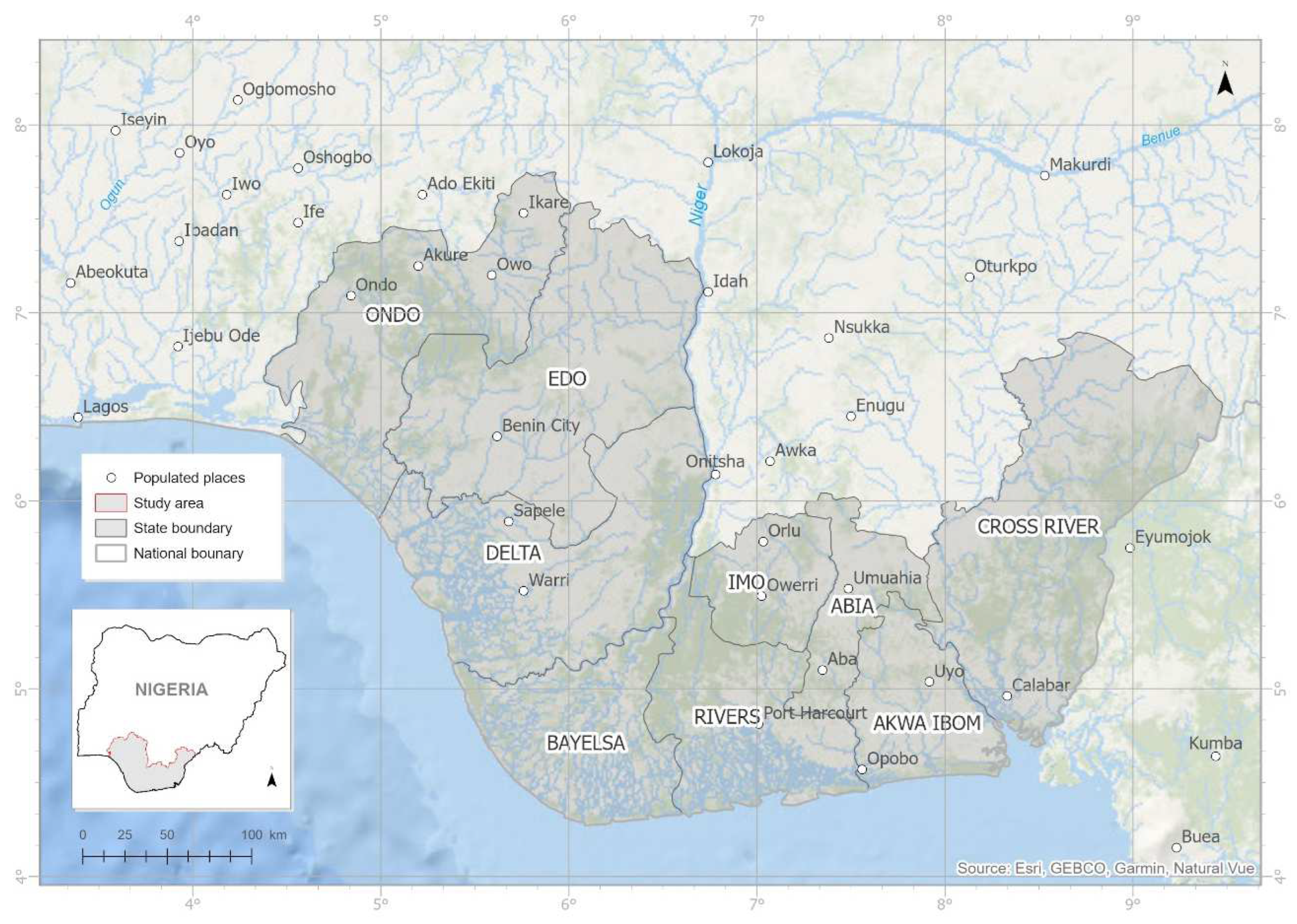
Figure 2.
Adopted workflow for mapping wetland change in the study area. The steps employed are highlighted in the six green headings (i.e., steps 1 to 6). Each section outlines the input data, primary output data, secondary output and tools employed.
Figure 2.
Adopted workflow for mapping wetland change in the study area. The steps employed are highlighted in the six green headings (i.e., steps 1 to 6). Each section outlines the input data, primary output data, secondary output and tools employed.
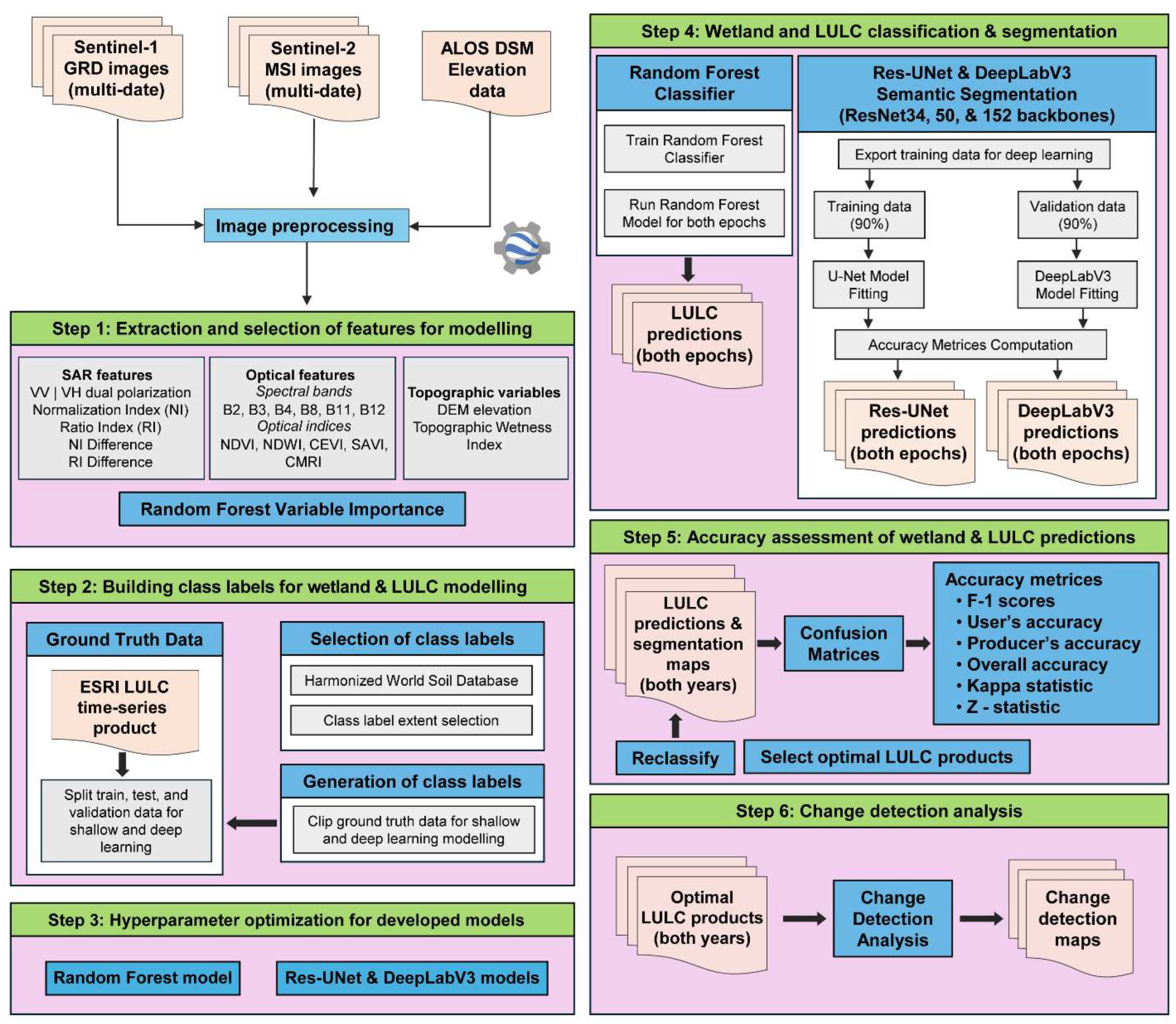
Figure 3.
Map of the Niger Delta showing the harmonized world soil database and the training and testing areas of interest used for training and validating the shallow and deep learning models developed in the study.
Figure 3.
Map of the Niger Delta showing the harmonized world soil database and the training and testing areas of interest used for training and validating the shallow and deep learning models developed in the study.
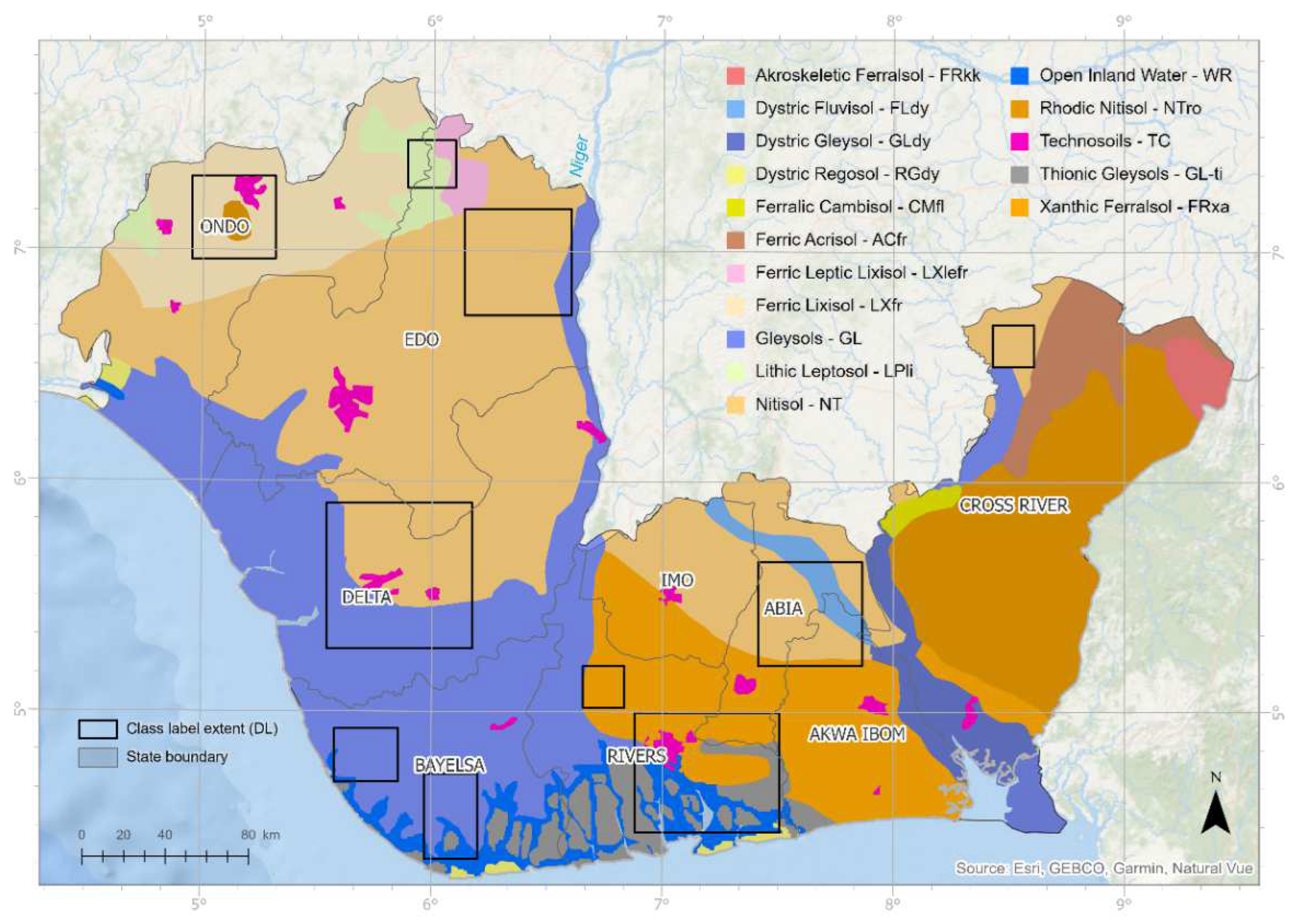
Figure 4.
Chart showing the random forest-derived variable importance test for the multi-source input variables analyzed in the study.
Figure 4.
Chart showing the random forest-derived variable importance test for the multi-source input variables analyzed in the study.
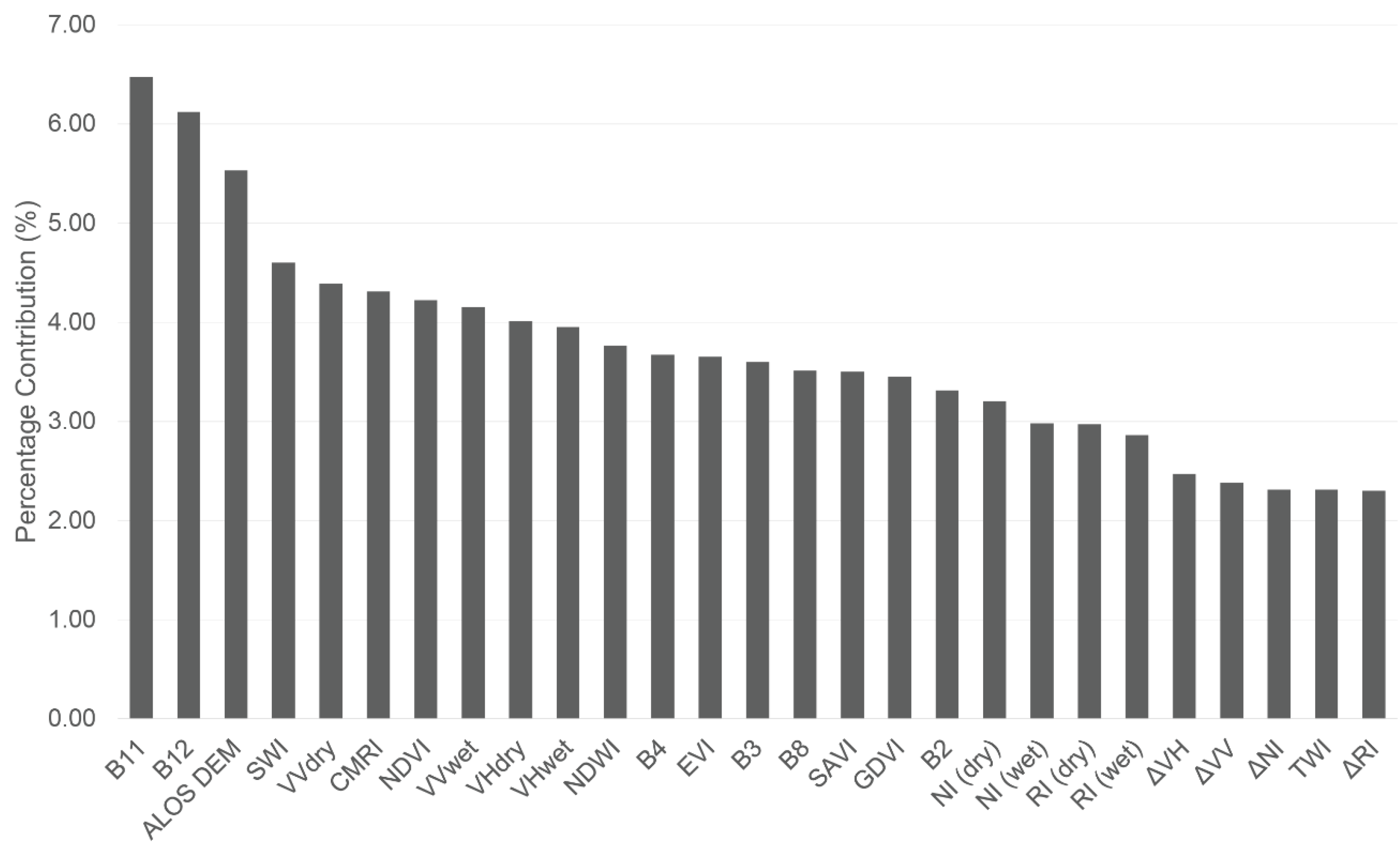
Figure 5.
Chart showing the inter-class F1 scores for the Res-UNet and DeepLabV3 deep learning models with similar backbones (ResNet34, ResNet50, and ResNet152) for both years (2019/2020 and 2021/2022) evaluated in the study.
Figure 5.
Chart showing the inter-class F1 scores for the Res-UNet and DeepLabV3 deep learning models with similar backbones (ResNet34, ResNet50, and ResNet152) for both years (2019/2020 and 2021/2022) evaluated in the study.
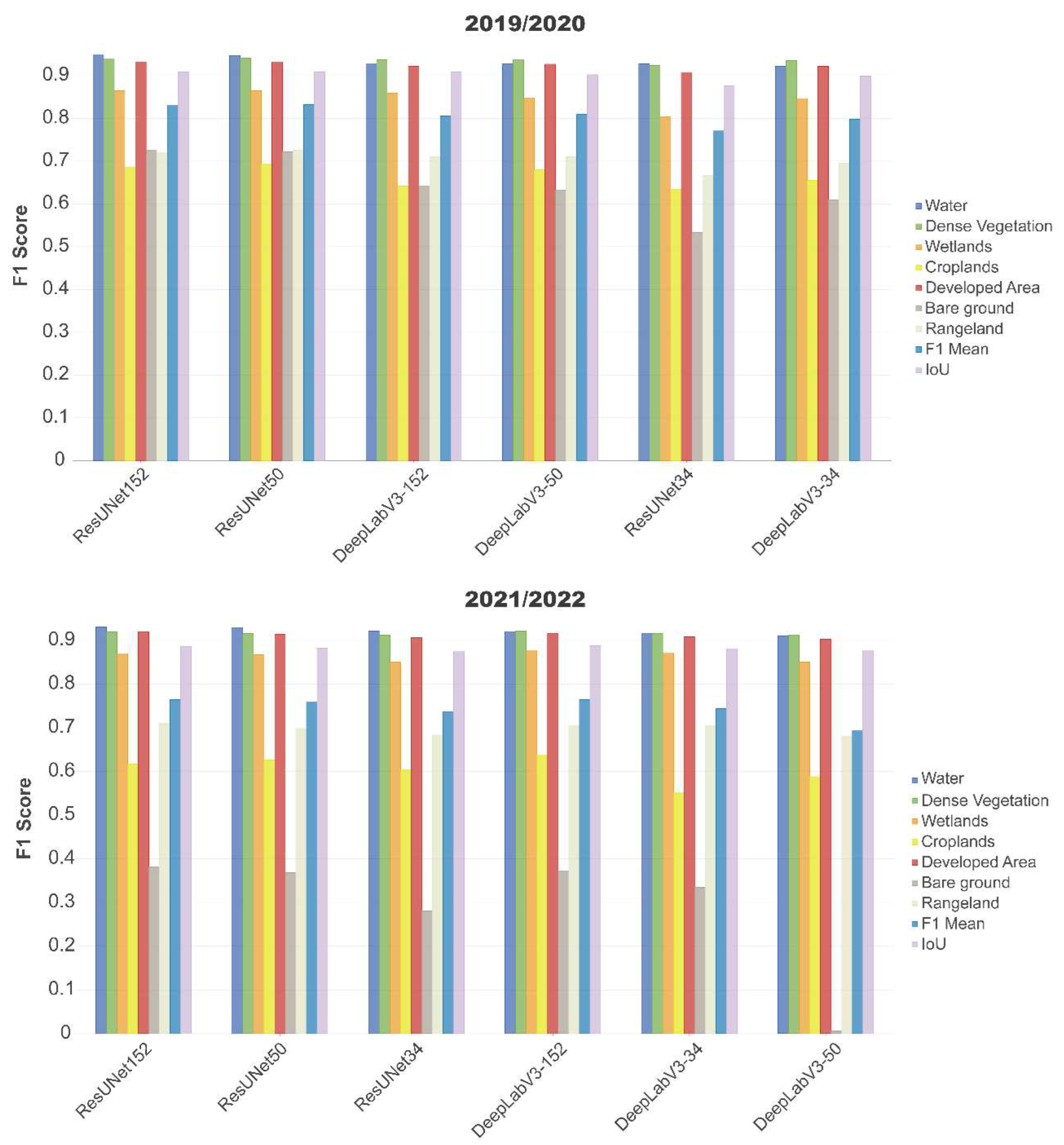
Figure 6.
Optimal deep learning models (Res-UNet with ResNet152 backbone) for (a) 2019/2020 and (b) 2021/2022.
Figure 6.
Optimal deep learning models (Res-UNet with ResNet152 backbone) for (a) 2019/2020 and (b) 2021/2022.
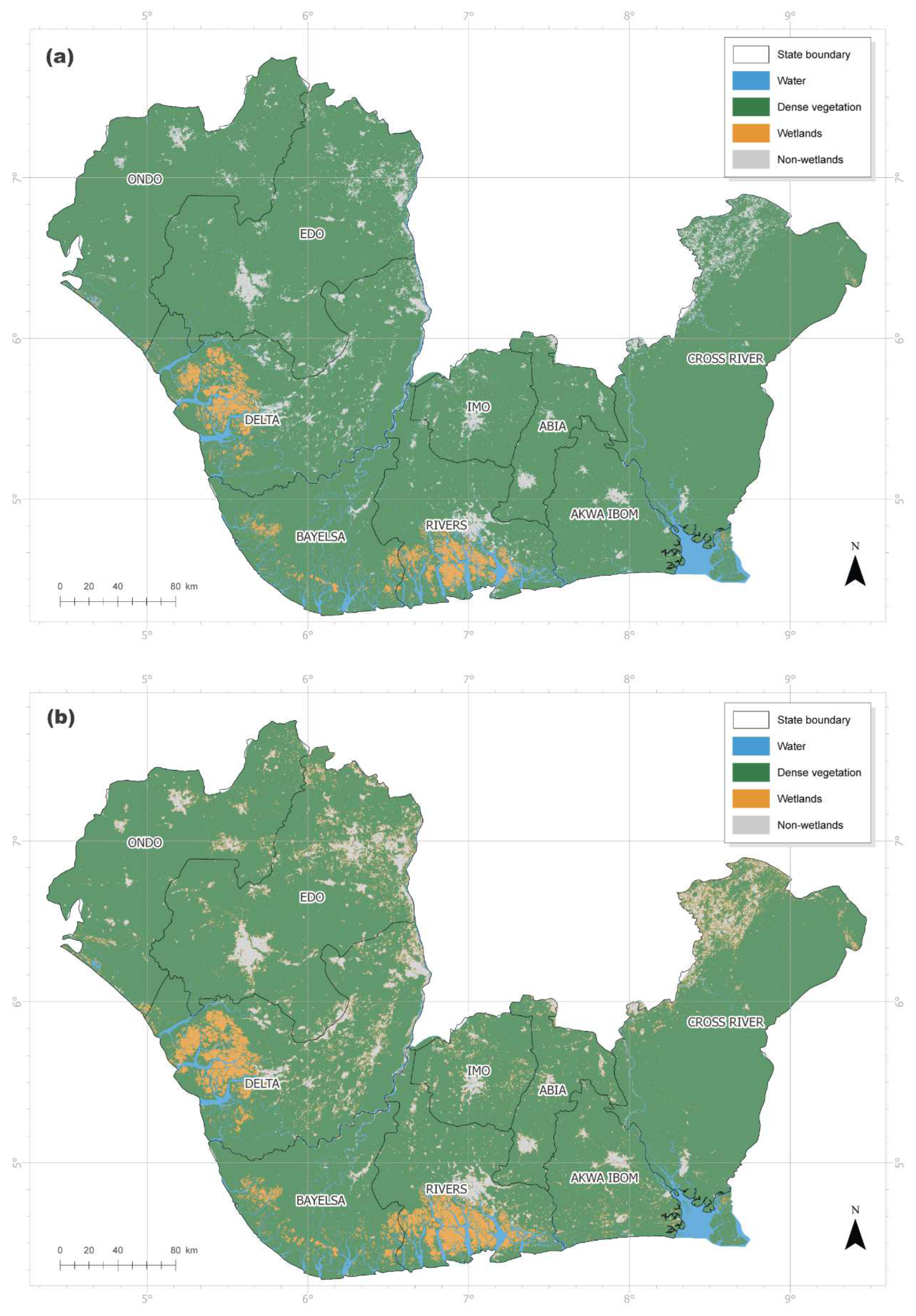
Figure 7.
Chart showing the spatial extent of wetland and non-wetland classes in the Niger Delta for 2019/2020 and 2021/2022.
Figure 7.
Chart showing the spatial extent of wetland and non-wetland classes in the Niger Delta for 2019/2020 and 2021/2022.

Figure 8.
Pie charts showing the proportion of (a) wetland loss and (b) wetland gain from 2019/2020 to 2021/2022 in the Niger Delta.
Figure 8.
Pie charts showing the proportion of (a) wetland loss and (b) wetland gain from 2019/2020 to 2021/2022 in the Niger Delta.
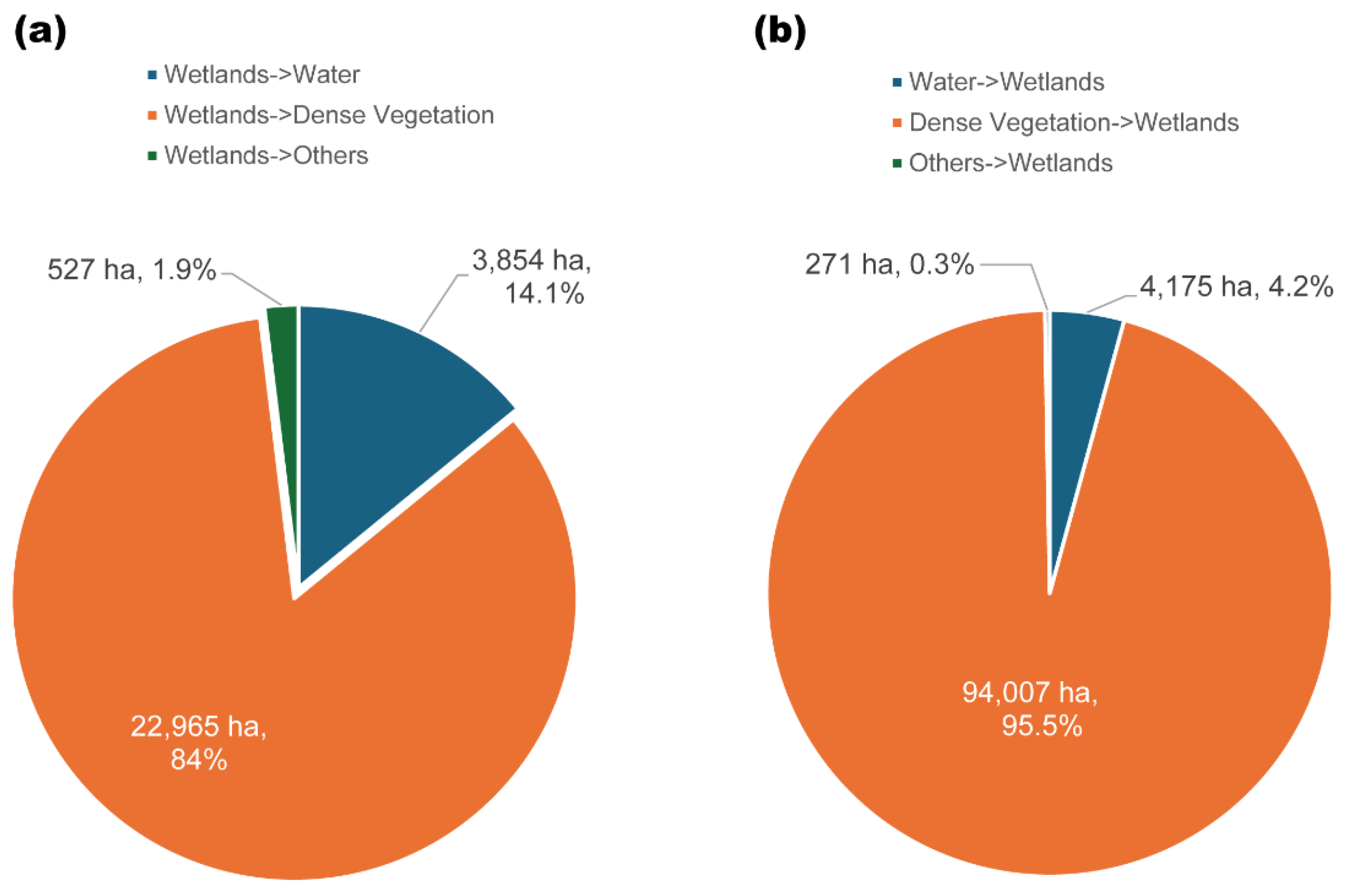
Figure 9.
Change detection map showing wetland dynamics between 2019/2020 and 2021/2022 based on the optimal Res-UNet deep learning models.
Figure 9.
Change detection map showing wetland dynamics between 2019/2020 and 2021/2022 based on the optimal Res-UNet deep learning models.
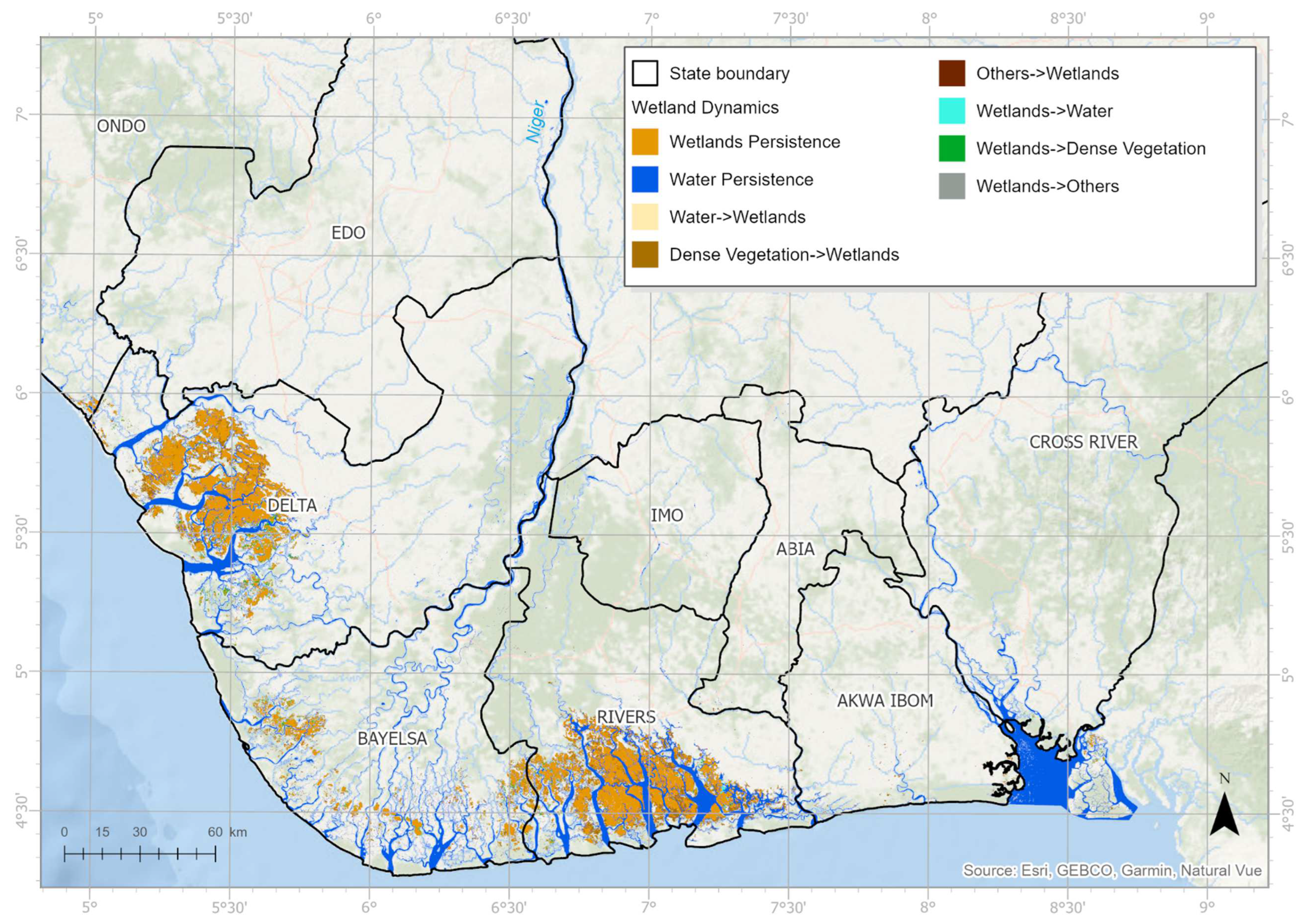
Figure 10.
Change detection hotspot maps showing wetland dynamics between 2019/2020 and 2021/2022 for parts of two states—Delta and River States in the Niger Delta based on the optimal Res-UNet deep learning models (Left images: 2019/2020 ResUNet152 prediction, Middle image: 2021/2022 ResUNet152 model prediction, and Right image: Change detection map based on both images). The insert map shows the spatial extent of two hotspot locations located in Delta and Rivers States.
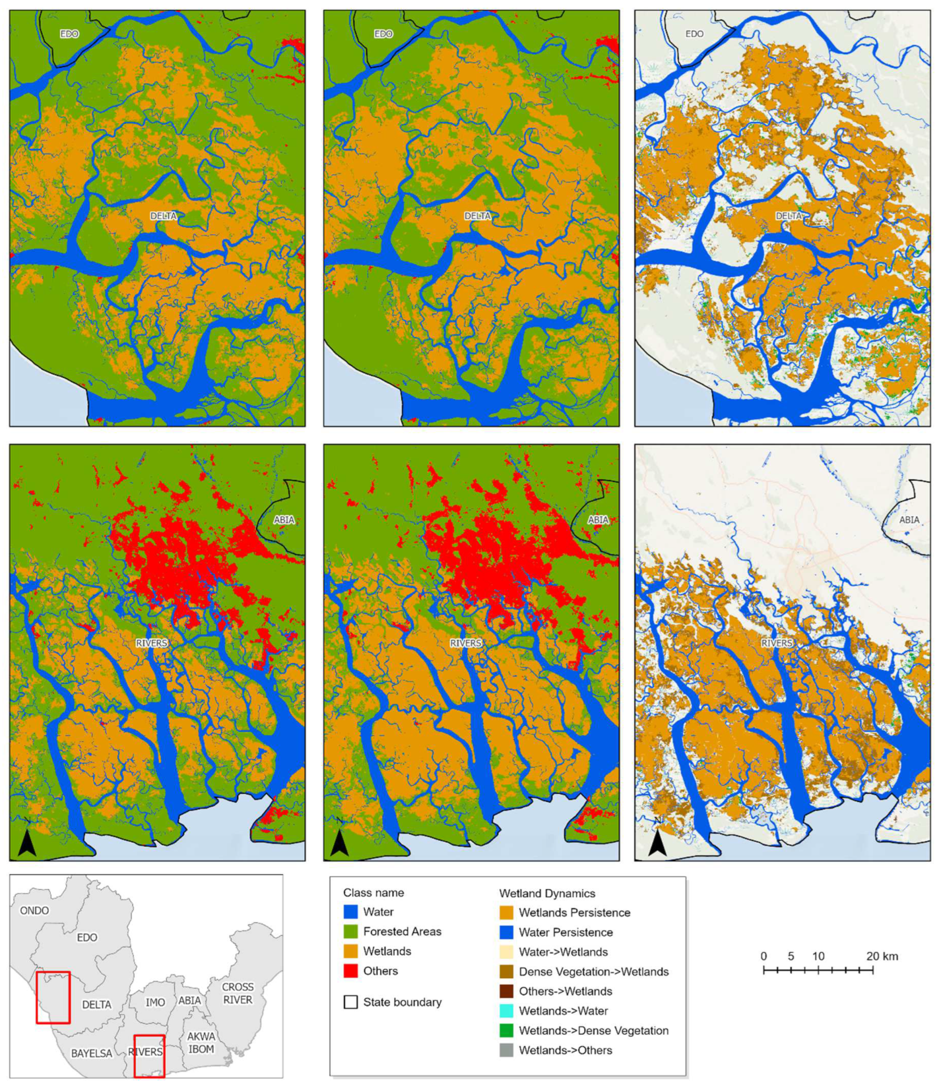
Figure 11.
Hydrological indicators to track impacts of extreme events on wetland dynamics. The SPEI shows (a) the proportion of areas under drought averaged over the study region and (b) temporal patterns of hydrological conditions between 2019 and 2023. The thick red dotted line in (a) is the period this study focuses on. The (c) anomalies in rainfall and the decomposition of TWS into (d) seasonal and (e) trend components are also indicated. The red dotted line in (b) is the drought threshold used for this study.
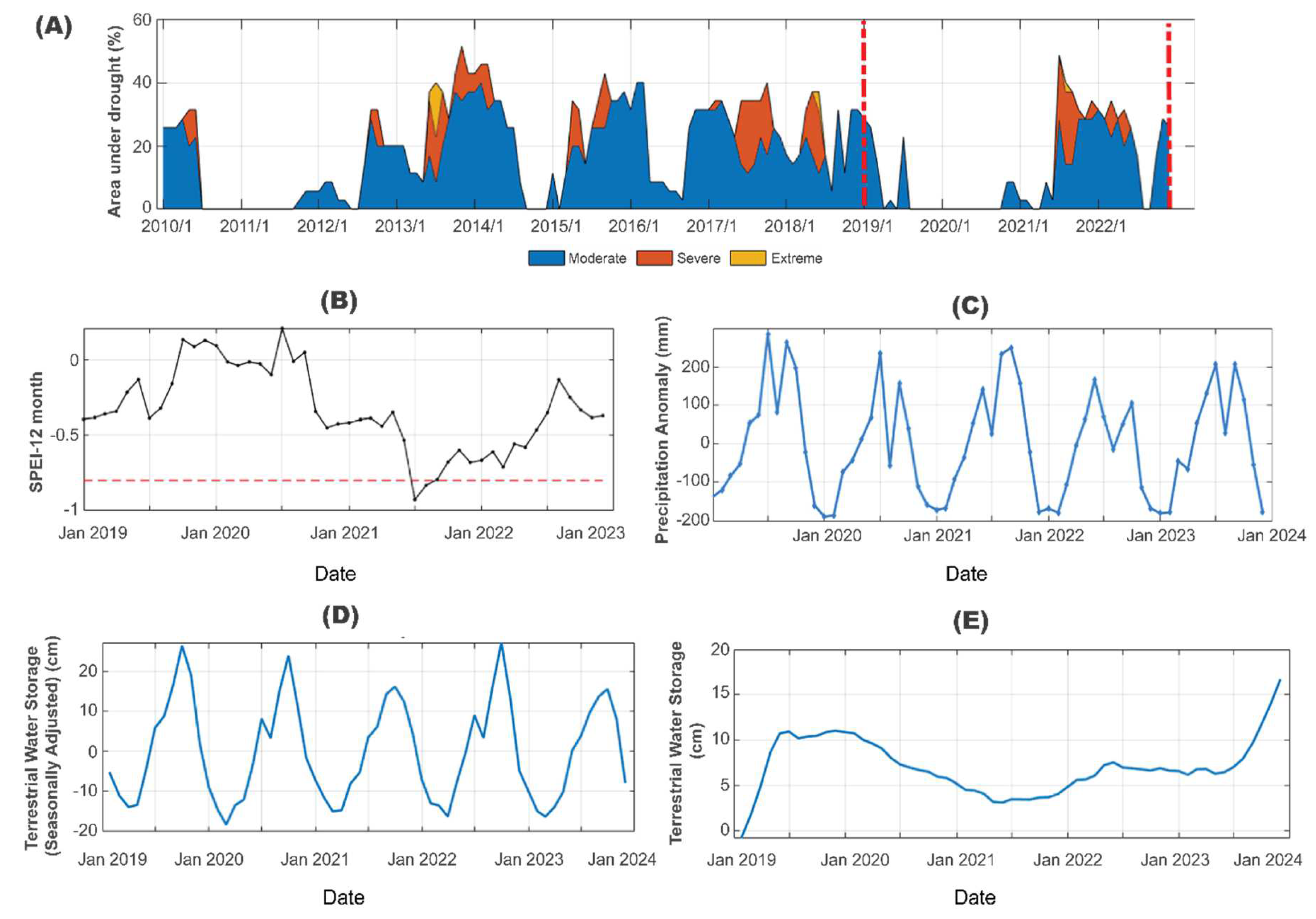
Figure 12.
Spatial patterns of the seasonally averaged annual standardized precipitation index (SPI) for January to March, April to June, July to September, and October to December for 2019 to 2022.
Figure 12.
Spatial patterns of the seasonally averaged annual standardized precipitation index (SPI) for January to March, April to June, July to September, and October to December for 2019 to 2022.
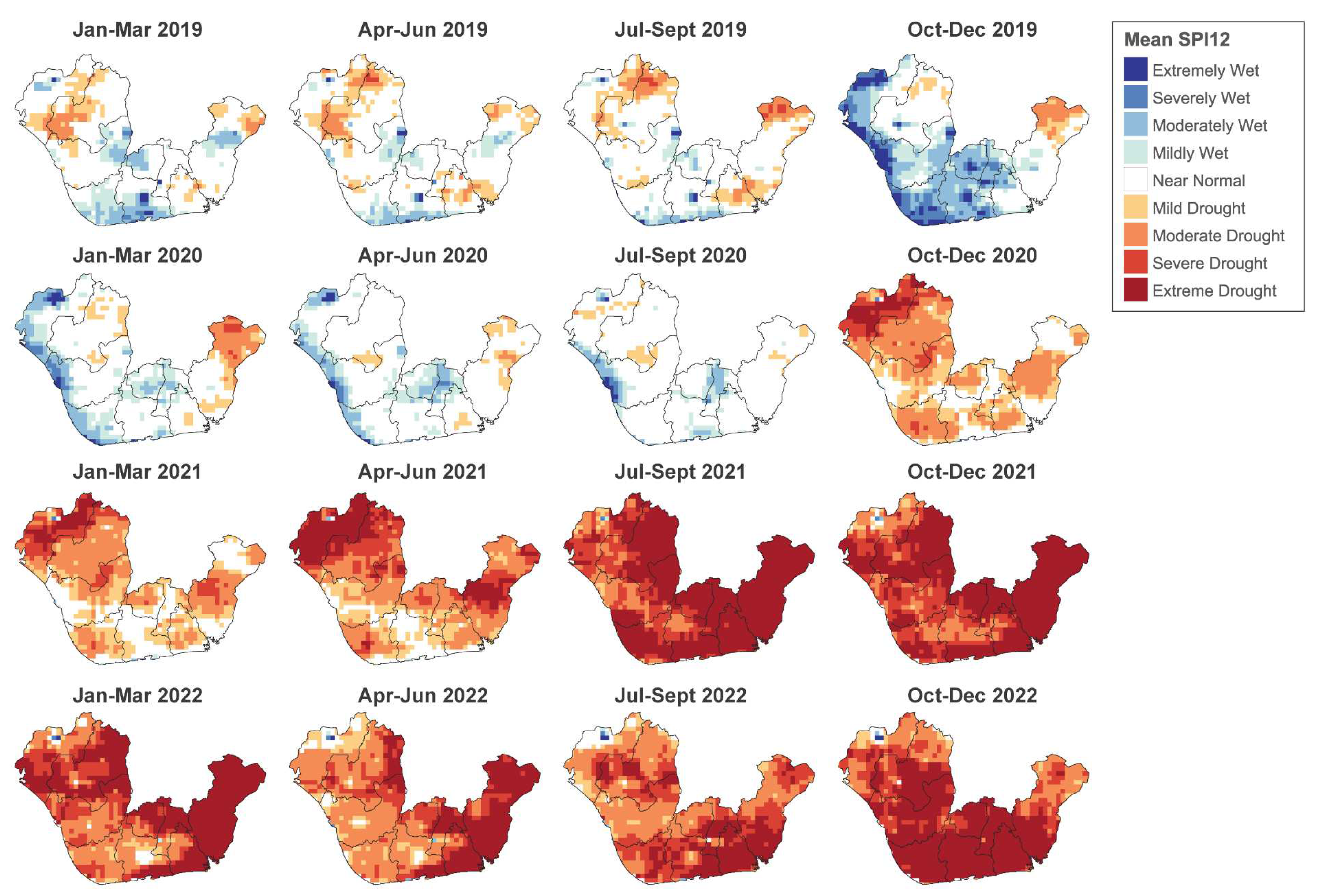

Table 1.
Sentinel-1, Sentinel-2, and ALOS DEM elevation data explored in the study (Where VH: Vertical transmit and horizontal receive polarization, VV: Vertical transmit and vertical receive polarization, dry: January to March; wet: April to July, late wet months: September to November, ΔNI: Normalization index seasonal difference (dry minus wet months), ΔRI: Ratio index seasonal difference (dry minus wet months), B: Band, B2: Blue band, B3: Green band, B4: Red band, B5: red edge-1 band, B8: near-infrared band, B11: shortwave infra-red-1 band, and B12: shortwave infra-red-2 band, NDVI: Normalized Difference Vegetation Index, NDWI: Normalized Difference Water Index, EVI: Enhanced Vegetation Index, SAVI: Soil Adjusted Vegetation Index (where L is the correction factor, and ranges between 0 and 1, a value of 0.5 was used in the study), SWI: Sentinel-2 Water Index, CMRI: Combined Mangrove Recognition Index, ALOS: Advanced Land Observing Satellite, DEM: Digital Elevation Model, and TWI: Topographic Wetness Index (where A is the upslope contributing area, and β is the local slope angle)).
| Satellite Sensor | Channels / Bands | Calculated indices |
|---|---|---|
| Sentinel-1 SAR data | Dual polarization channels: VVdry | VVwet | VVlate-wet VHdry | VHwet | VHlate-wet |
(for dry, wet, and late wet months) |
|
(for dry, wet, and late wet months) | ||
| Δ NI = NIdry − NIwet | ||
| Δ RI = RIdry − RIwet | ||
| Sentinel-2 optical data | Selected bands: B2, B3, B4, B5, B8, B11, and B12. |
|
Table 2.
Drought and flood classification based on Standardized Precipitation Evapotranspiration Index (SPEI) and Standardized Precipitation Index (SPI) values used in study.
Table 2.
Drought and flood classification based on Standardized Precipitation Evapotranspiration Index (SPEI) and Standardized Precipitation Index (SPI) values used in study.
| Category | Range for SPEI and SPI |
|---|---|
| Extreme Drought | -3.6 to -1.6 |
| Severe Drought | -1.6 to -1.3 |
| Moderate Drought | -1.3 to -0.8 |
| Mild Drought | -0.8 to -0.5 |
| Near Normal | -0.5 to 0.5 |
| Mildly Wet | 0.5 to 0.8 |
| Moderately Wet | 0.8 to 1.3 |
| Severely Wet | 1.3 to 1.6 |
| Extremely Wet | 1.6 to 3 |
Table 3.
Description of landcover class labels adopted in the study.
| FAO / ESRI Class Label | Study Class Label | Sample | Description |
|---|---|---|---|
| Water | Water |  |
These are areas predominantly covered by water throughout the year; they do not contain sparse vegetation, rock outcrops, or built-up features. Examples include rivers, lakes, ponds, oceans, and flooded salt plains. |
| Trees | Dense Vegetation or Forested areas |  |
These are dense vegetation areas, with heights of approximately 15 feet or higher and mostly closed or dense canopies. This land cover class encompasses dense or tall swamps and mangroves with temporary water or a canopy that is too thick to detect water underneath, as well as wooded vegetation and plantations. |
| Flooded vegetation | Wetlands |  |
Areas of any vegetation type with water intermixing for most of the year include seasonally flooded areas, characterized by a mixture of grass, shrubs, trees, and bare ground. Examples of this class are flooded mangroves and emergent vegetation. |
| Crops | Croplands |  |
Agricultural croplands in the study area include fallow plots of structured land, plantations, and fallow farmlands. |
| Built Area | Developed Areas |  |
These are human-made structures, such as dense villages, towns, or cities, major roads and rail networks, and homogeneous impervious surfaces (e.g., office buildings and residential housing). |
| Bare ground | Bare ground |  |
Rocky or bare soil areas with very sparse vegetation cover for the entire year. These areas are predominantly large expanses of land with limited or no vegetation cover. Examples in the region include exposed rocks or soil, mine sites, dried lake beds or dry salt flats. |
| Rangeland | Rangeland |  |
These are open areas predominantly covered in homogeneous grasses with relatively short vegetation. This class also consists of small or single-plant clusters dispersed across large landscapes, with exposed soil or rock elements. Examples of this class include scrub-filled clearings within dense forests, moderate to sparse bush cover, savannas with sparse grasses, trees or other plants, and shrubs. |
Table 4.
Inventory of training and validation data used for developing the random forest model.
| Class value | Class name | Count |
| 1 | Rangeland | 1000 |
| 2 | Wetlands | 400 |
| 3 | Croplands | 485 |
| 4 | Dense Vegetation | 675 |
| 5 | Bare ground | 106 |
| 6 | Developed Area | 751 |
| 7 | Water | 515 |
Table 5.
A list of learning rate parameters for deep learning models developed in the study.
| Period | Model | Backbone | Learning rate (min) | Learning rate (min) | Processing time (hrs) |
|---|---|---|---|---|---|
| 2019/2020 | Res-UNet | ResNet34 | 2.512E-06 | 0.0000251 | 5.0 |
| ResNet50 | 3.311E-05 | 0.0003311 | 14.3 | ||
| ResNet152 | 5.248E-06 | 0.0000525 | 35.2 | ||
| DeepLabV3 | ResNet34 | 2.089E-04 | 0.0020893 | 3.3 | |
| ResNet50 | 1.738E-04 | 0.0017378 | 5.0 | ||
| ResNet152 | 3.631E-04 | 0.0036080 | 34.0 | ||
| 2021/2022 | Res-UNet | ResNet34 | 7.586E-06 | 0.0000759 | 4.0 |
| ResNet50 | 4.365E-06 | 0.0000437 | 31.6 | ||
| ResNet152 | 2.754E-05 | 0.0002754 | 33.2 | ||
| DeepLabV3 | ResNet34 | 7.586E-04 | 0.0075858 | 3.6 | |
| ResNet50 | 1.097E-03 | 0.0109650 | 4.4 | ||
| ResNet152 | 2.512E-04 | 0.0025119 | 5.0 |
Table 6.
Results of McNermar’s test for the significant difference in overall accuracy generated for the Res-UNet154 deep learning model and random forest classification.
Table 6.
Results of McNermar’s test for the significant difference in overall accuracy generated for the Res-UNet154 deep learning model and random forest classification.
| Comparison | Z-score value | Significance level (%) |
| Res-UNet152 vs Random Forest (2019/2020) | 3.27 | 99% |
| Res-UNet152 vs Random Forest (2021/2022) | 4.32 | 99% |
Table 7.
Change detection results showing spatial changes of wetlands and non-wetland classes in the Niger Delta (where Dense veg = Dense vegetation).
Table 7.
Change detection results showing spatial changes of wetlands and non-wetland classes in the Niger Delta (where Dense veg = Dense vegetation).
| Class value | Class name | Class From | Class To | Area (ha) | % Change | Description |
| 1 | Wetlands | Wetlands | Wetlands | 250,099.5 | 1.3 | Unchanged wetlands |
| 2 | Water->Wetlands | Water | Wetlands | 4,174.9 | 8.7 | Wetland gain |
| 3 | Dense Veg ->Wetlands | Dense Veg | Wetlands | 94,007.3 | 90.8 | Wetland gain |
| 4 | Others->Wetlands | Others | Wetlands | 271.0 | 0.6 | Wetland gain |
| Total wetlands gain extent (ha) | 98,453.1 | 0.9 | ||||
| 5 | Wetlands->Water | Wetlands | Water | 3,853.5 | 15.3 | Wetland loss |
| 6 | Wetlands->Dense Veg | Wetlands | Dense Veg | 22,965.4 | 81.0 | Wetland loss |
| 7 | Wetlands->Others | Wetlands | Others | 527.2 | 3.7 | Wetland loss |
| Total wetland loss extent (ha) | 27,346.2 | 0.2 | ||||
| 8 | Water | Water | Water | 419,878.0 | 3.7 | Unchanged water |
| 9 | Dense Veg. | Dense Veg. | Dense Veg | 9,452,716.0 | 81.1 | Unchanged Dense Veg |
| 10 | Others | Others | Others | 452,944.7 | 4.6 | Unchanged other classes |
| 11 | Water->Dense Veg | Water | Dense Veg | 8,888.5 | 0.3 | Water loss |
| 12 | Water->Others | Water | Others | 3,346.6 | 0.1 | Water loss |
| 13 | Forested Areas->Water | Dense Veg | Water | 13,341.4 | 0.2 | Water gain |
| 14 | Others->Water | Others | Water | 1,997.7 | 0.1 | Water gain |
| 15 | Dense Veg->Others | Dense Veg | Others | 248,771.9 | 1.7 | Dense Veg loss |
| 16 | Others->Dense Veg | Others | Dense Veg | 59,053.6 | 5.1 | Dense Veg gain |
| Total non-wetland dynamics extent (ha) | 10,660,938.4 | 96.6 | ||||
| Total extent of Niger Delta extent (ha) | 11,036,837.2 | |||||
Disclaimer/Publisher’s Note: The statements, opinions and data contained in all publications are solely those of the individual author(s) and contributor(s) and not of MDPI and/or the editor(s). MDPI and/or the editor(s) disclaim responsibility for any injury to people or property resulting from any ideas, methods, instructions or products referred to in the content. |
© 2025 by the authors. Licensee MDPI, Basel, Switzerland. This article is an open access article distributed under the terms and conditions of the Creative Commons Attribution (CC BY) license (https://creativecommons.org/licenses/by/4.0/).
Copyright: This open access article is published under a Creative Commons CC BY 4.0 license, which permit the free download, distribution, and reuse, provided that the author and preprint are cited in any reuse.


