
Submitted:
23 September 2024
Posted:
24 September 2024
You are already at the latest version
Abstract
The influence of climate conditions and stable design on horses housed in single stalls can have significant effects, especially in regions with tropical savannah climates. A recent study observed variations in autonomic responses in horses housed in different stable designs during the summer, but there is limited information about their conditions during the monsoon. This study investigated the stable microenvironment and autonomic regulation of horses housed in different stable archi-tectures during the monsoon in a tropical savannah environment. Twenty-two horses were allo-cated to one of three stable architectures, each with varying stable microenvironments. The findings reveal that the heart rate variability (HRV) was lower in horses in a stable with a solid external wall and lower volume-to-horse ratio compared to those in a stable with a solid external wall but a higher volume-to-horse ratio or one without a solid external wall. Additionally, the study found that stable microenvironments and HRV modulation were correlated with stable architecture. Autonomic responses differed among horses in different stable architectures, indicating that stable microen-vironments and, to some extent, volume-to-horse ratio play a role in horses’ autonomic regulation. The findings have implications for improvements in housing and welfare in tropical savannah environments.
Keywords:
Air velocity
; Humidity
; Interior environment
; Monsoon
; Noxious gases
; Single-stall housing
; Stress responses
; Temperature
; Tropical savannah climate
; Welfare
1. Introduction
Horses have been selectively bred for various human-related activities, such as transportation, hunting, and sports [1,2]. Accordingly, they are exposed to multiple different forms of husbandry, including housing and management conditions, feeding protocols, physical activities, and preventive health care, all of which can impact their welfare [3,4,5,6]. It is generally believed that group housing in outdoor areas can promote the welfare of domestic horses by allowing for social interaction, grazing, and unrestrained movement, resembling the natural living conditions of feral horses [7,8,9]. However, concerns about maintaining feeding quality and the potential for horses to sustain injuries during outdoor housing have prompted some caretakers to opt for single-stall boxes as their preferred housing option [7,10,11,12].
Single-stall boxes have been used for routine accommodation of most sports horses in Western countries, varying from 32–90% across different nations [3,13,14,15,16]. Housing in a single-stall box is thought to facilitate husbandry practices regarding nutritional management, parasite control, and protection from atmospheric pollution [4,17]. Nevertheless, the adverse effects of single-stall housing persist, such as a lack of social relationships and natural feeding behaviour [18,19]. In addition, horses left unfed for given periods of the day may be prone to developing abnormal stereotypies, gastric ulcers, and colic [20,21]. Finally, isolation in single-stall housing is associated with the expression of stress-related behaviour in horses [6,22].
It is important to consider the impact of stable design on the welfare of domestic animals, especially in single-stall housing systems. Traditional single stalls with full partitions can limit interaction and social bonding [7]. Some designs address this issue by including a solid lower segment and a vertical or horizontal bar between adjacent boxes, permitting visual, auditory, and olfactory contact between neighbouring horses [23,24]. Additionally, climatic conditions play a significant role in animal welfare. For instance, in dairy farms, closed barn housing systems are more suitable for areas with high rainfall and temperate climates, whereas open housing facilities are recommended in tropical regions [25]. In colder climates, shelters provide protection from strong winds, precipitation, and radiation [26,27]. Accordingly, both the housing system and climatic conditions have the potential to impact the welfare of single-stalled horses.
According to the Köppen climate classification system [28], a tropical climate is defined by having an average temperature of 18 °C (64.4 °F) or higher in every month of the year, with significant precipitation of less than 60 mm (2.4 inches) in the driest month [29,30]. It is considered a harsh environment due to its characteristics of persistently high relative humidity and air temperature, which may significantly affect the optimal performance and welfare of animals, including horses [31,32,33,34].
Recent research has shown distinct stress responses in single-stalled horses within different stable designs, with those in open housing systems experiencing lower stress than those in closed systems, at least during the summer in tropical savannah climates [35]. However, there is a lack of information on how these factors affect horses and stable microclimates during the monsoon season in tropical savannah regions, which is characterised by increased precipitation and high humidity. Therefore, this study sought to investigate the variations in stable microclimate and autonomic regulation in horses housed under different stable architectures during the monsoon in a tropical savannah environment. We hypothesised that there may be differences in stable microclimate and horses’ autonomic regulation across three stable architectures during the monsoon in this region. Additionally, the study expects to establish a correlation between the stable’s microclimate and the horses’ autonomic responses.
2. Materials and Methods
2.1. Animals
We included 23 healthy horses (twelve geldings, one stallion, and ten mares, aged 14–26 and weighing 335–520 kg) from two similar management riding clubs located in a tropical savannah region in Thailand [36,37,38]. The selection included 14 horses from the Horse Lover’s Club in Pathum Thani (latitude: 13.99433, longitude: 100.68079) and nine from the House of Horse Riding Club in Bangkok (latitude: 13.81283, longitude: 100.78692). The horses were regularly trained for jumping or school riding on 3–4 days a week, with Mondays being their routine day off. Their diet consisted of 1–2 kg of commercial pellets divided into three even portions daily, along with ad libitum access to pangola hay and tap water. No therapeutic approaches had been administered to the horses within the 30 days leading up to the study. Any horse showing clinical signs of illness would have been excluded, but this was unnecessary. However, one horse from the House of Horse Riding Club became ill during the experiment; thus, 22 horses completed the study.
2.2. Experimental Protocols
The study was carried out at both riding clubs. As we needed the horses to be housed in their stables for a continuous 24-hour period, the experiments were conducted on three consecutive Mondays to mitigate the effect of routine activities that may misrepresent the horses’ autonomic modulation.
During the study, each horse was assigned to live in one of three stable architectures similar to the report described previously [35]. 1) Stable A. Eight horses (four geldings and four mares aged 20.8 ± 5.9 years and weighing 424.1 ± 57.0 kg) were accommodated in a stable with solid external walls made of brick, insulated with a plaster layer on the lower half to a height of 170 cm. The upper half was equipped with wire mesh and a small mesh net to prevent the entry of midges. The stable was 50 m long, 15 m wide, and 4 m high (stable volume: 3000 m3). Stable A had 20 independent 4 x 4 m single stalls, partitioned by solid walls at 170 cm in height, with multiple vertical bars above to allow visual contact between horses in adjacent stalls. A 4 m-wide corridor with front and back gates at each end was located between two rows of single stalls (Figure 1A). 2) Stable B. Six horses (two geldings and four mares aged 20.0 ± 2.3 years and weighing 458.5 ± 81.5 kg) were housed in a stable with solid external walls, similar to Stable A. However, Stable B consisted of only one row of 10 separate 4 x 4 m boxes with a one-sided aisle located in front of the boxes. Stable B was 50 m long, 7 m wide, and 4 m high (stable volume: 1,400 m3). The stable gates were located at each end of the aisle, perpendicular to the stable’s longitudinal axis (Figure 1B). 3) Stable C. Eight horses (five geldings, one stallion, and two mares aged 17.4 ± 4.7 years and weighing 415.7 ± 106.7 kg) were housed in a stable with similar characteristics and volume to stable A but without solid external walls. A mesh net was equipped at the roof edge of the stable, which could be rolled up to permit free air ventilation during the day and released to temporarily cover the stable at night (Figure 1C). In all stable setups, the front and back gates were fully open during the day and completely closed from 18:00–05:30. The bedding and manure were collected twice daily at 05:30 and 17:30 on the experimental days.
2.3. Data Acquisition
2.3.1. Environmental Parameters
Throughout the experiment, humidity and air temperature were measured using three sets of temperature and humidity data logger devices (TM-305U; Tenmars Electronics, Taipei, Taiwan). Two devices were positioned in the stable corridor approximately 60–70 cm from the floor, while one was placed outside the barns. The stables’ average humidity and air temperature were reported as percentages (%) and degrees Celsius (°C), respectively. Data were collected at 1-minute intervals and presented as average values of each consecutive 60-minute period over 24 hours (07.00 h on the first day to 07.00 h on the following day), during the day (07.00–18.00 h) and night (18.00–05.00 h).
Two anemometers (GM8902, BENETECH, Shenzhen, China) were installed within and outside the stables in the same direction to estimate the internal and external air velocity (m/s) during the experiment. Ammonia (NH3) concentrations were assessed inside the stables with two portable ammonia gas monitoring devices (SC-04 (NH3); Riken Keiki, Tokyo, Japan). Two pieces of the portable gas monitoring device (GX-3R; Riken Keiki, Tokyo, Japan) were placed inside each of the barns at heights of 60–70 cm from the floor to measure various gases inside the stables, specifically methane (CH4), hydrogen sulphide (H2S) carbon monoxide (CO), and oxygen (O2). The NH3, CO and H2S levels were expressed as parts per million (ppm), and O2 and CH4 were described as a percentage of the lower explosive limit (LEL), respectively. Data were exported at 1-minute intervals and reported as average values of each consecutive 60-minute period for 24 hours (as above).
2.3.2. Autonomic Regulation
Autonomic regulation in the horses was assessed by observing heart rate variability (HRV) using a Polar heart rate monitoring (HRM) device (Polar Electro Oy, Kempele, Finland), which includes a Polar equine belt for riding, the heart rate sensor (H10), and the Polar sports watch (Vantage V3). This HRM device has been shown to provide reliable HRV parameters in horses [39,40,41,42]. To conduct the HRV analysis, the belt, attached to the heart rate sensor (H10), was moistened with plain water, and ultrasound gel was applied to the electrode surface to facilitate signal transmission. It was then positioned around the horse’s chest with the sensor pocket on the middle left side. The sensor was wirelessly connected to the Polar sports watch to record mean beat-to-beat (RR) intervals during the experiment. After recording, the Polar sports watch was connected to the Polar FlowSync program (https://flow.polar.com/, accessed on 14 July 2024) to upload the RR interval data in CSV format. Subsequently, the data was further processed using the Kubios premium software (Kubios HRV Scientific; https://www.kubios.com/hrv-premium/, accessed on 14 July 2024) to compute HRV variables and generate reports in MATLAB MAT files. The automatic artefact correction algorithm was used to exclude artefacts and ectopic beats from the RR interval data. Additionally, segments identified as noise were removed from the HRV analysis using automatic noise detection, with the setting at medium, to ensure the accuracy of the HRV analysis. Smoothness priors were applied to eliminate nonstationarities in the RR intervals time series, and a cutoff frequency for trend removal was set at 0.035 Hz, as instructed in the user’s guidelines (https://www.kubios.com/downloads/Kubios_HRV Users_Guide.pdf, accessed on 14 July 2024).
The HRV variables were classified into four categories:
1) time domain results: mean RR intervals, mean heart rate (HR), standard deviation of normal-to-normal RR intervals (SDNN), root mean square of successive differences between RR intervals (RMSSD), triangular interpolation of normal-to-normal intervals (TINN), RR triangular index (RRTI), and stress index.
2) frequency domain results: very-low-frequency band (VLF; frequency band threshold 0.00–0.01 Hz), low-frequency band (LF; frequency band threshold 0.01–0.07 Hz), high-frequency band (HF; frequency band threshold 0.07–0.6 Hz), LF/HF ratio, and total power.
3) Nonlinear results: standard deviation of the Poincaré plot perpendicular to the line of identity (SD1), standard deviation of the Poincaré plot along the line of identity (SD2), and SD2/SD1 ratio.
4) autonomic nervous (ANS) system index: parasympathetic nervous system (PNS) index and sympathetic nervous system (SNS) index.
It is worth noting that the HRV variables may have been influenced by stable cleaning practices from 05:30 to 06:30 h, potentially distorting the genuine autonomic responses. Additionally, the feeding schedule for the horses at 05:00 h, 11:00 h, and 17:00 h may have caused arousal and associated behaviours. Due to these factors, the HRV data from 05:00–07:00, 10:50–11:10, and 16:50–17:10 were excluded from the analysis to ensure accurate HRV estimation. Consequently, the HRV variables were evaluated at 60-minute intervals, except during 10:00–11:00 h, 11:00–12:00 h, 16:00–17:00 h, and 17:00–18:00 h, which were assessed at 50-minute intervals. The evaluation was carried out from 07:00 h on the experimental days until 05:00 h the following day.
2.4. Data Analysis
The data were analysed using GraphPad Prism version 10.3.1 (GraphPad Software Inc, San Diego, USA). Due to missing data, the effects of independent group and time and the group-by-time interaction on modulation in air velocity, relative humidity, air temperature, and HRV variables were assessed using the mixed-effects model (restricted maximum likelihood: REML) with Greenhouse–Geisser correction. Subsequently, Tukey’s post-hoc test was employed for both within-group and between-group comparisons at specific time points. Normal distribution of the data was verified using the Shapiro–Wilk test when appropriate. Due to the data being non-normally distributed, variations in interior ammonia levels, horses’ age, and weight were assessed using the Kruskal–Wallis test, followed by Dunn’s multiple comparisons test. Spearman’s rank correlation (rs) was used to evaluate relationships among stable microclimate and HRV variables, with correlation coefficients categorised as weak (± 0.10 ≤ rs < ± 0.40), moderate (± 0.40 ≤ rs < ± 0.70), strong (± 0.70 ≤ rs < ± 0.90), or very strong (rs ≥ ± 0.90) [43]. The data were presented as means ± SD, and p < 0.05 was considered to be statistically significant.
3. Results
3.1. Air Velocity
Throughout the 24-hour measurement period, both the exterior and interior air velocity (AiV) exhibited fluctuations, as illustrated in Figures 2A and 2B. The exterior AiV in stable B was found to be comparable to that of stable C but significantly lower than in stable A during the day (p < 0.05). The exterior AiV was no different among stables at night but was lower than during the day across three stable architectures (p < 0.01–0.0001) (Figure 2C). The interior AiV was higher in stable C than in stables A and B during the day, with no significant difference at night (p < 0.001–0.0001). Specifically, only the interior AiV in stable C exhibited higher values during the day than at night (p < 0.0001) (Figure 2D).
3.2. Relative Humidity
The relative humidity (RH) showed the most variation during the day, both inside and outside stables B and C, as demonstrated in Figures 3A and 3B. The exterior RH in all stable architectures was lower during the day than at night (p < 0.001–0.0001). Additionally, stable C exhibited higher exterior RH than stables A and B during both day (p < 0.01–0.001) and night (p < 0.001–0.0001) (Figure 3C). The interior RH in stable C did not differ significantly from stable B during the day, but it was higher than that of stable A (p < 0.05). At night, the interior RH in stable C was also higher than in stables A and B (p < 0.0001). Notably, the interior RH was higher at night in stables A and C than during the day (Figure 3D). Despite lower exterior RH during the day (p < 0.001) (Figure 3C), the interior RH in stable B did not exhibit significant differences between day and night (Figure 3D).
3.3. Air Temperature
Similar to RH, the exterior and interior air temperature (AT) varied the most in stables B and C (Figure 4A and 4B). The AT in stable B was higher than in stables A and C during the day both outside (stable A vs B: p < 0.001; stable B vs C: p < 0.0001) and inside the stables (p < 0.05 for both comparison pairs). In contrast, it was higher in stable A than in stables B and C at night, both outside (p < 0.05 for both comparison pairs) and inside the stables (p < 0.0001 for both comparison pairs). Even though the exterior AT was higher during the day than at night in all stable architectures, only stables B and C showed higher interior AT during the day than at night (Figure 4C and 4D).
3.4. Levels of Noxious Gases
Ammonia levels were barely detected in stables A and C during the day but were mainly observed in all three stables at night (Figure 5A). However, there was no significant difference in the ammonia levels among the three stables during the day and night (Figures 5B and 5C). In addition, H2S, NH3, and CO were not detected within the stables, except for O2, which remained at a constant level of 20.9% over 24 hours.
3.5. Autonomic Regulation
Autonomic regulation was evaluated through the modulation of HRV variables as follows:
3.5.1. RR Intervals, HR, PNS Index, and SNS Index
The effects of group-by-time interaction and independent time were observed in the modifications of mean RR intervals (p < 0.0001 for both effects), mean HR (p = 0.0016 and p < 0.0001), PNS index (p = 0.0054 and p < 0.0001) and SNS index (p = 0.0013 and p < 0.0001) (Figure 6).
Mean RR intervals increased at night in stable A (23.00–05.00 h, compared to the values at 07.00–09.00 h and 18.00–19.00 h, p < 0.05–0.0001; 20.00–05.00 h, compared to the values at 11.00–12.00 h and 17.00–18.00 h, p < 0.05–0.0001). In stable B, mean RR intervals significantly reduced at 17.00–19.00 h (p < 0.05–0.0001, compared to the values at 07.00–11.00 h and 14.00–16.00 h) and then rose at night (21.00–05.00 h, compared to the values at 11.00–12.00 h and 17.00–19.00 h, p < 0.05–0.0001). The mean RR intervals in stable C were lower at 11.00–13.00 and 17.00–19.00 h compared to 07.00–08.00 h (p < 0.05–0.001) and then increased at night, similar to that of stables A and B (22.00–05.00 h, compared to 07.00–14.00 h and 15.00–19.00 h, p < 0.05–0.0001) (Figure 6A).
Mean HR reduced at night in stable A (01.00–05.00 h, compared to the values at 07.00–09.00 h, p < 0.05–0.01; 22.00–05.00 h, compared to the values at 11.00–12.00 h and 17.00–19.00 h, p < 0.05–0.0001). In stable B, the mean HR showed two peaks at 11.00–12.00 h (p < 0.05, compared to the value at 07.00–0.8.00 h) and 17.00–19.00 h (p < 0.05–0.0001, compared to the values at 07.00–11.00 h and 14.00–16.00 h). It finally decreased at night (21.00–05.00 h, compared to the values at 11.00–12.00 h and 17.00–19.00 h, p < 0.05–0.0001). The mean HR in stable C rose at 11.00–14.00 h (p < 0.05, compared to the value at 07.00–08.00 h) and eventually dropped at night (22.00–05.00 h, compared to the values at 11.00–14.00 h and 17.00–19.00 h, p < 0.05–0.0001). The mean HR in stable B was higher than in stable A and stable C at 17.00–18.00 h (stables A vs B, p < 0.05 and stable B vs C, p < 0.01) (Figure 6B).
PNS index increased at night in stable A (02.00–05.00 h, compared to the values at 07.00–09.00 h, p < 0.05–0.01; 23.00–05.00 h, compared to the values at 11.00–12.00 h and 17.00–18.00 h, p < 0.05–0.001). In stable B, the PNS index declined at 17.00–19.00 h (p < 0.05–0.0001, compared to the values at 07.00–11.00 h) before rising at night (21.00–05.00 h, compared to the values at 11.00–12.00 h and 17.00–19.00 h, p < 0.05–0.0001). The PNS index in stable C also increased at night (23.00–05.00 h, compared to the values at 08.00–09.00 h, 11.00–14.00 h and 17.00–19.00 h, p < 0.05–0.0001). The PNS index was higher in stable C than in stable A at 07.00–08.00 h (p < 0.05) (Figure 6C).
SNS index declined in stable A at night (02.00–05.00 h, compared to the values at 07.00–09.00 h; p < 0.05–0.01; 23.00–05.00 h, compared to the values at 11.00–12.00 h and 17.00–19.00 h, p < 0.05–0.0001). In stable B, the SNS index increased at 11.00–12.00 h (p < 0.01–0.0001, compared to the values at 07.00–10.00 h) and 17.00–19.00 h (p < 0.01–0.0001, compared to the values at 08.00–11.00 h). It then dropped at 20.00–05.00 h (p < 0.05–0.0001, compared to the values at 11.00–12.00 h and 17.00–19.00 h). The SNS index in stable C increased at 12.00–13.00 h (p < 0.05, compared to the values at 07.00–08.00 h) and 17.00–19.00 h (p < 0.05, compared to the values at 07.00–08.00 h). It later decreased to reach a significantly different value at night (22.00–05.00 h, compared to the values at 11.00–14.00 h and 17.00–19.00 h, p < 0.05–0.01) (Figure 6D).
3.5.2. SDNN, RMSSD, TINN, and RRTI
The independent group effect impacted SDNN and RMSSD modulation (p = 0.0133 and p = 0.0329, respectively). In the meantime, the group-by-time interaction and independent effect of time affected changes in TINN (p = 0.0008 and p = 0.0316). In contrast, independent group and time effects influenced RRTI modification (p = 0.0498, p < 0.0001) (Figure 7).
SDNN decreased in stable B at 15.00–16.00 h (p < 0.05, compared to the value at 08.00–09.00 h). The SDNN in stable B was higher than in stable A at 08.00–11.00 h (p < 0.05–0.01) and stable C at 08.00–09.00 h (p < 0.05). The SDNN was higher in stable C than in stable A at 11.00–12.00 h (p < 0.05) (Figure 7A). RMSSD in stable B was higher than stable A at 07.00–11.00 h (p < 0.05–0.01), 20.00–21.00 (p < 0.05), 01.00–02.00 h (p < 0.05), and 03.00–04.00 h (p < 0.05). The RMSSD was also higher in stable B than in stable C at 08.00–09.00 h (p < 0.05) (Figure 7B).
TINN reduced in stable B at 15.00–16.00 h (p < 0.05–0.01, compared to the values at 08.00–10.00 h). In contrast, it increased in stable C at 14.00–15.00 h (p < 0.05, compared to the value at 08.00–09.00 h) before dropping at 17.00–19.00 h (p < 0.05, compared to the value at 14.00.00–15.00 h). The TINN in stable B was higher than stable A at 08.00–11.00 h (p < 0.01–0.001) and stable C at 08.00–10.00 h (p < 0.05–0.01). The TINN was higher in stable C than in stable A at 11.00–12.00 h (p < 0.001), 14.00–15.00 h (p < 0.0001), and 15.00–16.00 h (p < 0.05) (Figure 7C). RRTI decreased in stable B at 15.00–16.00 h (p < 0.05, compared to the values at 07.00–08.00 h and 10.00–11.00 h), increasing at 19.00–20.00 h (p < 0.05, compared to the values at 15.00–16.00 h), and finally decreasing to reach baseline value afterwards. The RRTI in stable B was higher than in stables A and C at 08.00–09.00 h (p < 0.05 for both comparison pairs), 10.00–11.00 h (p < 0.05 for both comparison pairs), and 20.00–21.00 h (stable A vs B, p < 0.05; stable B vs C, p < 0.01) (Figure 7D).
3.5.3. VLF Band, LF Band, HF Band, LF/HF Ratio, and Total Power
There was an independent effect of time on change in the VLF band (p < 0.0001), while there was an independent effect of group on total power modulation (p = 0.0051). The independent effects of group and time, and the group-by-time interaction, had no effect on the LF band, HF band and LF/HF ratio, even though the group effect was almost significant on both the LF (p = 0.0867) and HF bands (p = 0.0877) (Figure 8A–8D).
The VLF band increased at 23.00–00.00 h and 01.00–04.00 h (p < 0.05–0.0001, compared to the values at 11.00–12.00 h and 17.00–18.00 h) (Figure 8A). Total power in stable B was higher than in stable A at 08.00–09.00 h (p < 0.01) and 20.00–21.00 h (p < 0.05), and than in stable C at 08.00–09.00 h (p < 0.05). It was also higher in stable C than in stable A at 11.00–12.00 h (p < 0.05) and 15.00–16.00 h (p < 0.05) (Figure 8D).
3.5.4. Stress Index, SD1, SD2, and SD2/SD1 Ratio
The independent effect of time and the group-by-time interaction on the stress index were significant (p = 0.0472 and p = 0.0040, respectively). In contrast, the independent effect of group affected changes in SD1 and SD2 (p = 0.0326 and p = 0.0413, respectively), while there was an independent effect of time on the SD2/SD1 ratio (p = 0.0007) (Figure 9).
The stress index increased in stable B at 11.00–12.00 h and 15.00–16.00 h (p < 0.05–0.01, compared to the value at 08.00–09.00 h). The stress index in stable A was higher than in stable B at 08.00–11.00 h (p < 0.05–0.01) and stable C at 11.00–12.00 h (p < 0.01). The stress index was also higher in stable B than in stable C at 11.00–12.00 h (p < 0.05) (Figure 9A).
SD1 in stable B was higher than in stable A at 07.00–11.00 h, 20.00–21.00 h, 01.00–02.00 h, and 03.00–04.00 h (p < 0.05 for all time points). It was also higher than in stable C at 08.00–09.00 h (p < 0.05) (Figure 9B). SD2 decreased at 15.00–16.00 h (p < 0.05, compared to the value at 08.00–09.00 h). The SD2 was higher in stable B than in stable A at 08.00–09.00 h (p < 0.05). In the meantime, it showed a higher value in stable C than in stable A at 11.00–12.00 h and 15.00–16.00 h (p < 0.05 for both time points) (Figure 9C). SD2/SD1 ratio decreased at 03.00–04.00 h (p < 0.05, compared to the value at 17.00–18.00 h) (Figure 9D).
3.6. Correlation Among Stable Microclimates and Horses’ HRV Variables
The correlation matrixes display the relationships between interior and exterior microclimates and Horses’ HRV variables for 22 hours (07.00–05.00 h) in the three stable architectures.
3.6.1. Interior vs Exterior Microclimates
Exterior AiV moderately correlated with RT (rs = –0.44, p = 0.040) and AiT (rs = 0.60, p = 0.003) in stable A. It showed a moderate correlation with RT (rs = –0.69, p < 0.0001) and a strong correlation with AiT (rs = 0.77, p < 0.0001) in stable B. The exterior AiV strongly correlated with RT (rs = –0.90, p < 0.0001) and AiT (rs = 0.89, p < 0.0001) in stable C. The interior and exterior AiV, RT, and AiT were strongly correlated in stables A (AiV: rs = 0.83, p < 0.0001; RT: rs = 0.91, p < 0.0001; AiT: rs = 0.72, p < 0.0001) and C (AiV: rs = 0.86, p < 0.0001; RT: rs = 0.92, p < 0.0001; AiT: rs = 0.93, p < 0.0001). Moderate correlations in AiV (rs = 0.52, p = 0.013) and RT (rs = 0.62, p = 0.002) were detected between interior and exterior microclimates in stable B, but the correlation for AiT was stronger (rs = 0.86, p < 0.0001) (Figure S1).
3.6.2. Interior Microclimate vs Horses’ HRV Variables in Stable A
The variables RH, AiT, and AiV significantly correlated within stable A (RH vs AiT: rs = –0.83, p < 0.0001; RH vs AiV: rs = –0.80, p < 0.0001; AiT vs AiV: rs = 0.67, p = 0.0007). They were also correlated with several HRV variables, including mean RR intervals (RH: rs = 0.84, p < 0.0001; AiT: rs = –0.56, p = 0.007; AiV: rs = –0.52, p = 0.012), mean HR (RH: rs = –0.84, p < 0.0001; AiT: rs = 0.55, p = 0.008; AiV: rs = 0.54, p = 0.010), RMSSD (RH: rs = 0.58, p = 0.005; AiT: rs = –0.48, p = 0.023; AiV: rs = –0.53, p = 0.012), stress index (RH: rs = –0.68, p = 0.001; AiT: rs = 0.55, p = 0.008; AiV: rs = 0.67, p = 0.001), SD1 (RH: rs = 0.58, p = 0.005; AiT: rs = –0.48, p = 0.023; AiV: rs = –0.53, p = 0.012), PNS index (RH: rs = 0.85, p < 0.0001; AiT: rs = –0.59, p < 0.004; AiV: rs = –0.58, p = 0.005), and SNS index (RH: rs = –0.84, p < 0.0001; AiT: rs = 0.59, p = 0.004; AiV: rs = 0.58, p = 0.004).
Furthermore, RH was independently correlated with the VLF band (rs = 0.46, p = 0.029) and SD2/SD1 ratio (rs = –0.48, p = 0.024), while AiV displayed an additional correlation with SDNN (rs = –0.55, p = 0.008), total power band (rs = –0.46, p = 0.030), and SD2 (rs = –0.47, p = 0.028). Ammonia levels were correlated with RH (rs = 0.48, p = 0.025), AiT (rs = –0.44, p = 0.038), AiV (rs = –0.46, p = 0.031), RMSSD (rs = 0.59, p = 0.004), and SD1 (rs = 0.59, p = 0.004) (Figure 10).
3.6.3. Interior Microclimate vs Horses’ HRV Variables in Stable B
Significant correlations were mainly observed between AiT and various variables, including RH (rs = –0.62, p = 0.002), ammonia levels (rs = –0.57, p = 0.006), mean RR intervals (rs = –0.48, p = 0.002), mean HR (rs = 0.48, p = 0.023), SDNN (rs = –0.46, p = 0.029), RMSSD (rs = –0.62, p = 0.002), TINN (rs = –0.60, p = 0.003), SI (rs = 0.51, p = 0.016), LF band (rs = –0.44, p = 0.039), HF band (rs = 0.44, p = 0.039), SD1 (rs = –0.62, p = 0.002), PNS index (rs = –0.64, p = 0.001), and SNS index (rs = 0.61, p = 0.002). However, RH showed a correlation with a few HRV variables, including LF band (rs = 0.54, p = 0.009), HF band (rs = –0.54, p = 0.009), and SD2 (rs = 0.44, p = 0.039). Additionally, ammonia levels exhibited a correlation with mean RR intervals (rs = 0.52, p = 0.013), mean HR (rs = –0.45, p = 0.038), PNS index (rs = 0.50, p = 0.019), and SNS index (rs = –0.43, p = 0.043). No correlation was observed between AiV and other variables in stable B (Figure 11).
3.6.4. Interior Microclimate vs Horses’ HRV Variables in Stable C
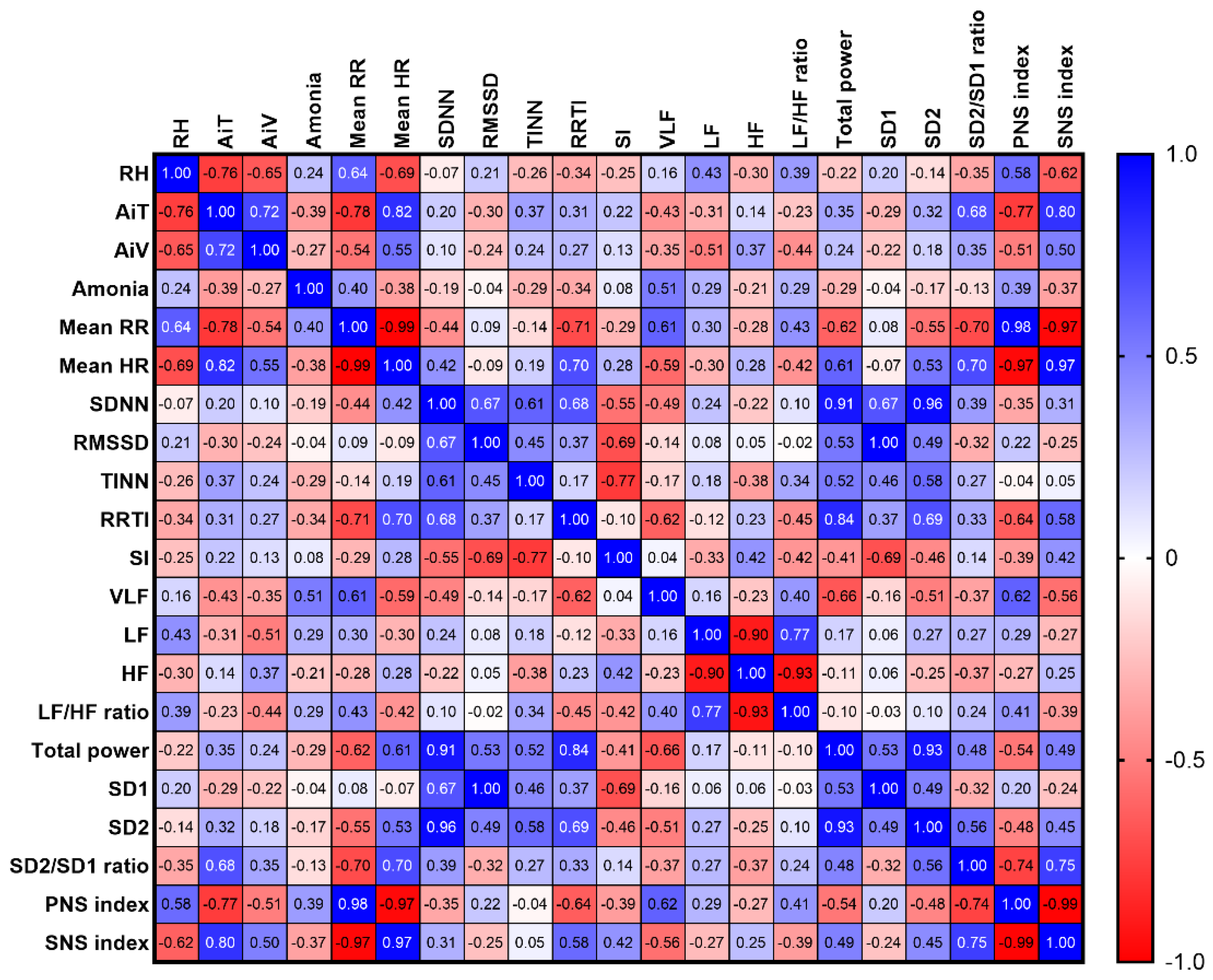
The variables RH, AiT, and AiV were correlated in stable C (RH vs AiT: rs = –0.76, p < 0.0001; RH vs AiV: rs = –0.65, p = 0.001; AiT vs AiV: rs = 0.72, p = 0.0001). Additionally, RH, AiT, and AiV showed simultaneous correlations with mean RR intervals (RH: rs = 0.64, p = 0.001; AiT: rs = –0.78, p < 0.0001; AiV: rs = –0.54, p = 0.009), mean HR (RH: rs = –0.69, p = 0.0004; AiT: rs = 0.82, p < 0.0001; AiV: rs = 0.55, p = 0.008), PNS index (RH: rs = 0.58, p = 0.005; AiT: rs = –0.77, p < 0.0001; AiV: rs = –0.51, p = 0.016), and SNS index (RH: rs = –0.62, p = 0.002; AiT: rs = 0.80, p < 0.0001; AiV: rs = 0.50, p = 0.019).
Moreover, RH was independently correlated with the LF band (rs = 0.43, p = 0.043), while AiT was independently correlated with the VLF band (rs = –0.43, p = 0.047) and SD2/SD1 ratio (rs = 0.68, p < 0.0001). On the other hand, AiV showed independent correlations with the LF band (rs = –0.51, p = 0.016) and LF/HF ratio (rs = –0.44, p = 0.040). Additionally, ammonia levels correlated only with the VLF band (rs = 0.51, p = 0.015) (Figure 12).
4. Discussion
The study explored how stable microenvironments and horses’ autonomic regulation were affected by single-stall housing in different stable designs during the monsoon season in a tropical savannah environment. Key findings included: 1) variations in stable microenvironments (AiV, RT, and AiT) and HRV modulation across different stable architectures; 2) higher interior AiV in stable C than in stables A and B during the day, with a similar pattern at night; 3) higher interior RT in stable C during the day compared to stable A, and this was higher than both stables A and B at night; 4) lower interior AiT in stable C than stable B during the day, and conversely lower than stables A and B at night; 5) increased mean RR and PNS index, corresponding to decreased mean HR and SNS index during the night in horses across all three stable architectures; 6) lower values of several HRV variables in stable A than stable B, and to a lesser extent than stable C; 7) correlations between stable microenvironments and various HRV variables in stable A and stable C; and 8) AiT being the only factor correlating with HRV variables in stable B. These findings suggest that stable microenvironmental variations significantly influence horses’ autonomic responses when housed in different stable architectures during monsoons in a tropical savannah environment.
We found a diurnal fluctuation in the exterior microclimate, encompassing air velocity, relative humidity, and air temperature within and among three stable structures. Interestingly, the interior microclimate also varied during the day and was associated with the exterior environment across the three stable architectures. These findings are consistent with existing literature, indicating that outdoor conditions play a significant role in shaping the stable microclimate in tropical environments [44,45,46]. However, the strength of correlation varied significantly between the different stable architectures, aligning with previous reports indicating that the connection between interior and exterior conditions differs based on building types in tropical climates [46].
While the interior and exterior air temperatures were strongly correlated across all three stable architectures in the present study, the impact of outdoor air velocity and relative humidity on these parameters varied within the three stables. Specifically, the design of the stable gates in stables A and C allowed more external air to flow through the central aisle, leading to a strong correlation between interior and exterior air velocity and relative humidity in these stables. Conversely, the stable gates perpendicular to the aisle limited the external air flow into stable B, resulting in a moderate correlation among these parameters. Notably, a broad correlation was observed between the interior and exterior environments in stable C, indicating a similarity between the exterior and interior conditions in this stable. These results support the idea that different stable architectures impact the variation in interior microclimate differently in a tropical savannah environment.
Ammonia was found inside the stables, especially at night, which aligns with the former literature [47] and the previous report on the same setting in the summer season [35]. Nevertheless, no variation in ammonia levels was detected among stables in the present study, contrasting with a former experiment showing significant variation in levels among stable designs during the summer season [35]. This discrepancy might result from the impact of interior air temperature variation between seasons, as it has been reported that temperature changes and ammonia levels are correlated when using straw bedding [48]. These results suggested that specific seasons impact the modulation of ammonia levels in tropical environments. Despite increasing at night, ammonia levels (0–4 ppm) in the three stable architectures were below the recommended maximum of 20 ppm in the stable, indicating no effect on horse welfare during this study [49].
In the realm of animal welfare research, HRV variables are commonly utilised to assess stress and autonomic responses in horses during transportation [50,51,52,53,54,55], shoeing protocols [56], training [57,58,59], and various exercise regimens in equestrian sports [60,61,62,63,64]. HRV refers to the fluctuation in time intervals between successive heartbeats during the cardiac cycle [65,66]. This variation is regulated by the interplay between sympathetic and parasympathetic (vagal) activities affecting the sinoatrial node of the heart [66,67]. Various HRV variables are employed to discern specific autonomic responses. For instance, changes in RMSSD, HF band, and SD1 reflect short-term fluctuations in inter-beat intervals following vagal activity [65,66]. Decreases in these variables indicate reduced vagal activity [63,64,68]. Meanwhile, modifications in RR intervals, SDNN, LF band, and SD2 reflect long-term variations in inter-beat intervals influenced by both sympathetic and vagal components [65,66,69,70]. Additionally, alterations in the TINN and RRTI mirror the overall variation in inter-beat intervals [71]. High HRV signifies predominant vagal activity, indicating good adaptability to environmental and psychological challenges [67,72,73]. Conversely, low HRV suggests reduced vagal influence, corresponding to sympathetic dominance and potentially serving as a marker for a state of disorder [74]. In the current study, HRV analysis was employed to assess autonomic regulation and, by extension, stress responses due to its user-friendly nature and non-invasive impact on horses’ regular activity. Increases in RR intervals and PNS index, accompanied by decreases in HR and SNS index, were observed, indicating an elevation in vagal tone concurrent with reduced sympathetic tone in horses at night. These findings are consistent with previous research reporting heightened vagal activity in horses during the night as a result of circadian rhythm [35,55,75,76].
We also found differences in the modulation of various HRV variables between stable architectures. Despite seasonal variations, the HRV variables were consistently lower in horses in stable A compared to stables B and C, similar to the findings in the summer season [35]. These findings suggest that stable architectures may have a more significant impact on HRV modulation than environmental conditions in a tropical savannah climate. Interestingly, stables A and B both had solid external walls, but HRV modulation was lower in stable A than in stable B. One possible explanation for this difference could be the stables’ volume-to-horse ratios. Stable B contained ten single boxes but only housed seven horses, resulting in a ratio of 200 m3 per horse. On the other hand, stable A housed 20 horses in 20 single boxes, resulting in a ratio of 150 m3 per horse. The lower ratio in stable A may have contributed to the lower HRV modulation compared to stable B. It is plausible that the lower number of horses, corresponding to a higher volume-to-horse ratio in stable B, led to decreased manure and urine production, subsequently reducing relative humidity, particularly at night (Figure 3). As a result, the stable volume-to-horse ratio must be considered, in addition to the stable architecture, when assessing the effects on autonomic modulation in horse housing in tropical environments. Therefore, the study implies that horses experienced more stress when housed in a stable with a solid external wall and a lower stable volume-to-horse ratio.
The impact of stable design on stable microclimate variation and horses’ autonomic responses has been thoroughly studied during the monsoon and dry summer seasons. However, the influence of these factors during the dry winter season in a tropical setting remains uncertain. Further research is necessary to identify the most appropriate stable designs for specific seasons in tropical environments. One limitation of the study was that same-day experiments were unavailable in all stable architectures due to insufficient devices for recording HRV and environmental parameters. This issue led to observed variations in the exterior environment among the three stables, which subsequently affected the interior microclimate and likely influenced the autonomic responses of the horses housed in those stables. While there were no significant differences in age and weight range among the horses, differences in individual characteristics and socialisation between stables may have also impacted their autonomic regulation. Therefore, cautious interpretation is essential when comparing the autonomic responses of horses among the three stables.
5. Conclusions
The exterior environment showed diurnal variation, which in turn affected the interior environments of the three stable types. These interior changes had different effects on the autonomic responses of horses housed within the stables. During the monsoon season in a tropical savannah environment, horses in the stable with a solid external wall and lower volume-to-horse ratio exhibited lower autonomic responses, indicating more stress compared to those in either the stable with a solid external wall but higher volume-to-horse ratio or the stable without a solid external wall. These findings offer valuable insights into the distinct autonomic regulation in horses within different stable architectures and could aid in the development of stable management practices to safeguard horse welfare during monsoons in tropical regions.
Supplementary Materials
The following supporting information can be downloaded at the website of this paper posted on Preprints.org. https://www.doi.org/10.6084/m9.figshare.27054571, Figure S1: Correlation between interior and exterior air velocity, relative humidity, and air temperature.
Author Contributions
Conceptualisation, methodology, software, validation, formal analysis, investigation, resources, data curation: C.P., K.S., K.L., T.W., and M.C.; writing—original draft preparation: T.W. and M.C.; writing—review and editing: T.W. and M.C.; visualisation: C.P., K.S., K.L., T.W., and M.C.; supervision and project administration: T.W. and M.C.; funding acquisition: C.P., T.W., and M.C. All authors have read and agreed to the published version of the manuscript.
Funding
This research and the APC were funded by the Faculty of Veterinary Medicine, Kasetsart University (grant number: VET.KU2024-16).
Institutional Review Board Statement
This study was conducted according to the guidelines of the Declaration of Helsinki and approved by the Ethics Committee of the Institutional Animal Care and Use Committee, Kasetsart University (ACKU65-VET-084).
Informed Consent Statement
Informed consent was obtained from the owners of all horses involved in the study.
Data Availability Statement
The data that support the findings of this study are available at https://www.doi.org/10.6084/m9.figshare.27054571 (accessed on 18 August 2024). The other information not provided in the repository platform is available from the corresponding authors, Metha Chanda and Thita Wonghanchao, upon reasonable request.
Acknowledgements
We are grateful to Vaewratt Kamonkon, director of the Horse Lover’s Club, and Chalermcharn Yotviriyapanit, director of the House of Horses Riding Club, for rendering the facilities available and for allowing us to conduct this experiment on their horses.
Conflicts of Interest
The authors declare no conflicts of interest.
References
- Orlando, L. The evolutionary and historical foundation of the modern horse: lessons from ancient genomics. Annu. Rev. Genet. 2020, 54, 563–581. [Google Scholar] [CrossRef] [PubMed]
- Klecel, W.; Martyniuk, E. From the Eurasian Steppes to the Roman Circuses: a review of early development of horse breeding and management. Animals 2021, 11. [Google Scholar] [CrossRef] [PubMed]
- Visser, E.K.; Neijenhuis, F.; de Graaf-Roelfsema, E.; Wesselink, H.G.M.; de Boer, J.; van Wijhe-Kiezebrink, M.C.; Engel, B.; van Reenen, C.G. Risk factors associated with health disorders in sport and leisure horses in the Netherlands1. J. Anim. Sci 2014, 92, 844–855. [Google Scholar] [CrossRef]
- Dalla Costa, E.; Dai, F.; Lebelt, D.; Scholz, P.; Barbieri, S.; Canali, E.; Minero, M. Initial outcomes of a harmonised approach to collect welfare data in sport and leisure horses. Animal 2017, 11, 254–260. [Google Scholar] [CrossRef]
- Thorne, J.B.; Goodwin, D.; Kennedy, M.J.; Davidson, H.P.B.; Harris, P. Foraging enrichment for individually housed horses: Practicality and effects on behaviour. Appl. Anim. Behav. Sci. 2005, 94, 149–164. [Google Scholar] [CrossRef]
- Visser, E.K.; Ellis, A.D.; Van Reenen, C.G. The effect of two different housing conditions on the welfare of young horses stabled for the first time. Appl. Anim. Behav. Sci. 2008, 114, 521–533. [Google Scholar] [CrossRef]
- Dai, F.; Dalla Costa, E.; Minero, M.; Briant, C. Does housing system affect horse welfare? The AWIN welfare assessment protocol applied to horses kept in an outdoor group-housing system: The ‘parcours’. Anim. Welf. 2023, 32, e22. [Google Scholar] [CrossRef]
- Hartmann, E.; Søndergaard, E.; Keeling, L.J. Keeping horses in groups: A review. Appl. Anim. Behav. Sci. 2012, 136, 77–87. [Google Scholar] [CrossRef]
- Leme, D.P.; Parsekian, A.B.H.; Kanaan, V.; Hötzel, M.J. Management, health, and abnormal behaviors of horses: A survey in small equestrian centers in Brazil. J. Vet. Behav. 2014, 9, 114–118. [Google Scholar] [CrossRef]
- Bachmann, I.; Stauffacher, M. [Housing and use of horses in Switzerland: a representative analysis of the status quo]. Schweiz. Arch. Tierheilkd. 2002, 144, 331–347. [Google Scholar] [CrossRef]
- Henderson, A.J.Z. Don’t fence me in: managing psychological well being for elite performance horses. J. Appl. Anim. Sci. 2007, 10, 309–329. [Google Scholar] [CrossRef]
- Fraser, D. Understanding animal welfare. Acta Vet. Scand. 2008, 50, S1. [Google Scholar] [CrossRef]
- Larsson, A.; Müller, C.E. Owner reported management, feeding and nutrition-related health problems in Arabian horses in Sweden. Livest. Sci. 2018, 215, 30–40. [Google Scholar] [CrossRef]
- Hockenhull, J.; Creighton, E. The day-to-day management of UK leisure horses and the prevalence of owner-reported stable-related and handling behaviour problems. Anim. Welf. 2015, 24, 29–36. [Google Scholar] [CrossRef]
- Hotchkiss, J.W.; Reid, S.W.J.; Christley, R.M. A survey of horse owners in Great Britain regarding horses in their care. Part 1: Horse demographic characteristics and management. Equine Vet. J. 2007, 39, 294–300. [Google Scholar] [CrossRef]
- Yngvesson, J.; Rey Torres, J.C.; Lindholm, J.; Pättiniemi, A.; Andersson, P.; Sassner, H. Health and body conditions of riding school horses housed in groups or kept in conventional tie-stall/box housing. Animals 2019, 9. [Google Scholar] [CrossRef] [PubMed]
- Ruet, A.; Lemarchand, J.; Parias, C.; Mach, N.; Moisan, M.-P.; Foury, A.; Briant, C.; Lansade, L. Housing horses in individual boxes is a challenge with regard to welfare. Animals 2019, 9. [Google Scholar] [CrossRef]
- Chaplin, S.J.; Gretgrix, L. Effect of housing conditions on activity and lying behaviour of horses. Animal 2010, 4, 792–795. [Google Scholar] [CrossRef]
- Søndergaard, E.; Ladewig, J. Group housing exerts a positive effect on the behaviour of young horses during training. Appl. Anim. Behav. Sci. 2004, 87, 105–118. [Google Scholar] [CrossRef]
- Hoffman, C.J.; Costa, L.R.; Freeman, L.M. Survey of feeding practices, supplement use, and knowledge of equine nutrition among a subpopulation of horse owners in New England. J. Equine Vet. Sci. 2009, 29, 719–726. [Google Scholar] [CrossRef]
- Hudson, J.M.; Cohen, N.D.; Gibbs, P.G.; Thompson, J.A. Feeding practices associated with colic in horses. AVMA 2001, 219, 1419–1425. [Google Scholar] [CrossRef] [PubMed]
- Pessoa, G.O.; Trigo, P.; Mesquita Neto, F.D.; Lacreta Junior, A.C.C.; Sousa, T.M.; Muniz, J.A.; Moura, R.S. Comparative well-being of horses kept under total or partial confinement prior to employment for mounted patrols. Appl. Anim. Behav. Sci. 2016, 184, 51–58. [Google Scholar] [CrossRef]
- Gmel, A.I.; Zollinger, A.; Wyss, C.; Bachmann, I.; Briefer Freymond, S. Social box: influence of a new housing system on the social interactions of stallions when driven in pairs. Animals 2022, 12. [Google Scholar] [CrossRef]
- Gehlen, H.; Krumbach, K.; Thöne-Reineke, C. Keeping stallions in groups—species-appropriate or relevant to animal welfare? Animals 2021, 11. [Google Scholar] [CrossRef]
- Roland, L.; Drillich, M.; Klein-Jöbstl, D.; Iwersen, M. Invited review: Influence of climatic conditions on the development, performance, and health of calves. J. Dairy Sci. 2016, 99, 2438–2452. [Google Scholar] [CrossRef] [PubMed]
- Mejdell, C.M.; Bøe, K.E.; Jørgensen, G.H.M. Caring for the horse in a cold climate—Reviewing principles for thermoregulation and horse preferences. Appl. Anim. Behav. Sci. 2020, 231, 105071. [Google Scholar] [CrossRef]
- Mejdell, C.M.; Bøe, K.E. Responses to climatic variables of horses housed outdoors under Nordic winter conditions. Can. J. Anim. Sci. 2005, 85, 307–308. [Google Scholar] [CrossRef]
- contributors, W. Köppen climate classification. Wikipedia, The Free Encyclopedia 2024. [Google Scholar]
- Beck, H.E.; Zimmermann, N.E.; McVicar, T.R.; Vergopolan, N.; Berg, A.; Wood, E.F. Present and future Köppen-Geiger climate classification maps at 1-km resolution. Sci. Data 2018, 5, 180214. [Google Scholar] [CrossRef]
- Peel, M.C.; Finlayson, B.L.; Mcmahon, T.A. Updated world map of the Köppen-Geiger climate classification. Hydrology and Earth System Sciences Discussions 2007, 4, 439–473. [Google Scholar] [CrossRef]
- Oke, O.E.; Uyanga, V.A.; Iyasere, O.S.; Oke, F.O.; Majekodunmi, B.C.; Logunleko, M.O.; Abiona, J.A.; Nwosu, E.U.; Abioja, M.O.; Daramola, J.O.; et al. Environmental stress and livestock productivity in hot-humid tropics: Alleviation and future perspectives. J. Therm. Biol. 2021, 100, 103077. [Google Scholar] [CrossRef] [PubMed]
- Nardone, A.; Ronchi, B.; Lacetera, N.; Bernabucci, U. Climatic effects on productive traits in livestock. Vet. Res. Commun. 2006, 30, 75–81. [Google Scholar] [CrossRef]
- Silanikove, N. Effects of heat stress on the welfare of extensively managed domestic ruminants. Livest. Prod. Sci. 2000, 67, 1–18. [Google Scholar] [CrossRef]
- Val, A.L.; De Almeida-Val, V.M.F.; Randall, D.J. Tropical environment. In Fish Physiology; Academic Press: 2005; Volume 21, pp. 1–45.
- Poochipakorn, C.; Wonghanchao, T.; Sanigavatee, K.; Chanda, M. Stress responses in horses housed in different stable designs during summer in a tropical savanna climate. Animals 2024, 14. [Google Scholar] [CrossRef]
- contributors, W. Tropical savanna climate. Wikipedia, The Free Encyclopedia 2024, 1220733028. [Google Scholar]
- Kottek, M.; Grieser, J.; Beck, C.; Rudolf, B.; Rubel, F. World map of the Köppen-Geiger climate classification updated. 2006, 15, 259–263, https://ui.adsabs.harvard.edu/link_gateway/2006MetZe..15..259K/10.1127/0941-2948/2006/0130.
- Khedari, J.; Sangprajak, A.; Hirunlabh, J. Thailand climatic zones. Renew. Energy 2002, 25, 267–280. [Google Scholar] [CrossRef]
- Frippiat, T.; van Beckhoven, C.; Moyse, E.; Art, T. Accuracy of a heart rate monitor for calculating heart rate variability parameters in exercising horses. J. Equine Vet. Sci. 2021, 104, 103716. [Google Scholar] [CrossRef]
- Kapteijn, C.M.; Frippiat, T.; van Beckhoven, C.; van Lith, H.A.; Endenburg, N.; Vermetten, E.; Rodenburg, T.B. Measuring heart rate variability using a heart rate monitor in horses (Equus caballus) during groundwork. Front. Vet. Sci. 2022, 9, 939534. [Google Scholar] [CrossRef]
- Ille, N.; Erber, R.; Aurich, C.; Aurich, J. Comparison of heart rate and heart rate variability obtained by heart rate monitors and simultaneously recorded electrocardiogram signals in nonexercising horses. J. Vet. Behav. 2014, 9, 341–346. [Google Scholar] [CrossRef]
- Mott, R.; Dowell, F.; Evans, N. Use of the Polar V800 and Actiheart 5 heart rate monitors for the assessment of heart rate variability (HRV) in horses. Appl. Anim. Behav. Sci. 2021, 241, 105401. [Google Scholar] [CrossRef]
- Schober, P.; Boer, C.; Schwarte, L.A. Correlation coefficients: appropriate use and interpretation. Anesth. Analg. 2018, 126. [Google Scholar] [CrossRef] [PubMed]
- Tumlin, K.; Liu, S.; Park, J.-H. Framing future of work considerations through climate and built environment assessment of volunteer work practices in the United States Equine Assisted Services. Int. J. Environ. Res. Public Health 2021, 18. [Google Scholar] [CrossRef] [PubMed]
- McGill, S.; Coleman, R.; Jackson, J.; Tumlin, K.; Stanton, V.; Hayes, M. Environmental spatial mapping within equine indoor arenas. Front. Anim. Sci. 2023, 4. [Google Scholar] [CrossRef]
- Pan, J.; Tang, J.; Caniza, M.; Heraud, J.-M.; Koay, E.; Lee, H.K.; Lee, C.K.; Li, Y.; Nava Ruiz, A.; Santillan-Salas, C.F.; et al. Correlating indoor and outdoor temperature and humidity in a sample of buildings in tropical climates. Indoor Air 2021, 31, 2281–2295. [Google Scholar] [CrossRef]
- Kwiatkowska-Stenzel, A.; Sowińska, J.; Witkowska, D. Analysis of noxious gas pollution in horse stable air. J. Equine Vet. Sci. 2014, 34, 249–256. [Google Scholar] [CrossRef]
- Fleming, K.; Hessel, E.F.; Van den Weghe, H.F. Gas and particle concentrations in horse stables with individual boxes as a function of the bedding material and the mucking regimen. J. Anim. Sci. 2009, 87, 3805–3816. [Google Scholar] [CrossRef]
- Janczarek, I.; Wilk, I.; Wiśniewska, A.; Kusy, R.; Cikacz, K.; Frątczak, M.; Wójcik, P. Effect of air temperature and humidity in a stable on basic physiological parameters in horses. Animal Sci. Genet. 2020, 16, 55–65. [Google Scholar] [CrossRef]
- Schmidt, A.; Möstl, E.; Wehnert, C.; Aurich, J.; Müller, J.; Aurich, C. Cortisol release and heart rate variability in horses during road transport. Horm. Behav. 2010, 57, 209–215. [Google Scholar] [CrossRef]
- Schmidt, A.; Hödl, S.; Möstl, E.; Aurich, J.; Müller, J.; Aurich, C. Cortisol release, heart rate, and heart rate variability in transport-naive horses during repeated road transport. Domest. Anim. Endocrinol. 2010, 39, 205–213. [Google Scholar] [CrossRef]
- Schmidt, A.; Biau, S.; Möstl, E.; Becker-Birck, M.; Morillon, B.; Aurich, J.; Faure, J.M.; Aurich, C. Changes in cortisol release and heart rate variability in sport horses during long-distance road transport. Domest. Anim. Endocrinol. 2010, 38, 179–189. [Google Scholar] [CrossRef]
- Lertratanachai, S.; Poochipakorn, C.; Sanigavatee, K.; Huangsaksri, O.; Wonghanchao, T.; Charoenchanikran, P.; Lawsirirat, C.; Chanda, M. Cortisol levels, heart rate, and autonomic responses in horses during repeated road transport with differently conditioned trucks in a tropical environment. PLoS One 2024, 19, e0301885. [Google Scholar] [CrossRef] [PubMed]
- Munsters, C.C.; de Gooijer, J.W.; van den Broek, J.; van, Oldruitenborgh; Oosterbaan, M.S. Heart rate, heart rate variability and behaviour of horses during air transport. Vet. Rec. 2013, 172, 15–15. [Google Scholar] [CrossRef]
- Ohmura, H.; Hobo, S.; Hiraga, A.; Jones, J.H. Changes in heart rate and heart rate variability during transportation of horses by road and air. Am. J. Vet. Res. 2012, 73, 515–521. [Google Scholar] [CrossRef]
- Huangsaksri, O.; Wonghanchao, T.; Sanigavatee, K.; Poochipakorn, C.; Chanda, M. Heart rate and heart rate variability in horses undergoing hot and cold shoeing. PLoS One 2024, 19, e0305031. [Google Scholar] [CrossRef] [PubMed]
- Cottin, F.; Barrey, E.; Lopes, P.; Billat, V. Effect of repeated exercise and recovery on heart rate variability in elite trotting horses during high-intensity interval training. Equine Vet. J. 2006, 38, 204–209. [Google Scholar] [CrossRef] [PubMed]
- Cottin, F.; Médigue, C.; Lopes, P.; Petit, E.; Papelier, Y.; Billat, V.L. Effect of exercise intensity and repetition on heart rate variability during training in elite trotting horse. Int. J. Sports Med. 2005, 26, 859–867. [Google Scholar] [CrossRef]
- Hammond, A.; Sage, W.; Hezzell, M.; Smith, S.; Franklin, S.; Allen, K. Heart rate variability during high-speed treadmill exercise and recovery in Thoroughbred racehorses presented for poor performance. Equine Vet. J. 2023, 55, 727–737. [Google Scholar] [CrossRef]
- Becker-Birck, M.; Schmidt, A.; Lasarzik, J.; Aurich, J.; Möstl, E.; Aurich, C. Cortisol release and heart rate variability in sport horses participating in equestrian competitions. J. Vet. Behav. 2013, 8, 87–94. [Google Scholar] [CrossRef]
- Ille, N.; von Lewinski, M.; Erber, R.; Wulf, M.; Aurich, J.; Möstl, E.; Aurich, C. Effects of the level of experience of horses and their riders on Cortisol release, heart rate and heart-rate variability during a jumping course. Anim. Welf. 2013, 22, 457–465. [Google Scholar] [CrossRef]
- Szabó, C.; Vizesi, Z.; Vincze, A. Heart rate and heart rate variability of amateur show jumping horses competing on different levels. Animals 2021, 11, 693. [Google Scholar] [CrossRef]
- Huangsaksri, O.; Sanigavatee, K.; Poochipakorn, C.; Wonghanchao, T.; Yalong, M.; Thongcham, K.; Srirattanamongkol, C.; Pornkittiwattanakul, S.; Sittiananwong, T.; Ithisariyanont, B.; et al. Physiological stress responses in horses participating in novice endurance rides. Heliyon 2024, 10. [Google Scholar] [CrossRef] [PubMed]
- Sanigavatee, K.; Poochipakorn, C.; Huangsaksri, O.; Wonghanchao, T.; Yalong, M.; Poungpuk, K.; Thanaudom, K.; Chanda, M. Hematological and physiological responses in polo ponies with different field-play positions during low-goal polo matches. PLoS One 2024, 19, e0303092. [Google Scholar] [CrossRef]
- Von Borell, E.; Langbein, J.; Després, G.; Hansen, S.; Leterrier, C.; Marchant-Forde, J.; Marchant-Forde, R.; Minero, M.; Mohr, E.; Prunier, A. Heart rate variability as a measure of autonomic regulation of cardiac activity for assessing stress and welfare in farm animals—A review. Physiol. Behav. 2007, 92, 293–316. [Google Scholar] [CrossRef]
- Stucke, D.; Große Ruse, M.; Lebelt, D. Measuring heart rate variability in horses to investigate the autonomic nervous system activity – Pros and cons of different methods. Appl. Anim. Behav. Sci. 2015, 166, 1–10. [Google Scholar] [CrossRef]
- Shaffer, F.; Ginsberg, J.P. An overview of heart rate variability metrics and norms. Front. Public Health 2017, 258. [Google Scholar] [CrossRef] [PubMed]
- Muñoz, A.; Castejón-Riber, C.; Castejón, F.; Rubio, D.M.; Riber, C. Heart rate variability parameters as markers of the adaptation to a sealed environment (a hypoxic normobaric chamber) in the horse. J. Anim. Physiol. Anim. Nutr. (Berl.) 2019, 103, 1538–1545. [Google Scholar] [CrossRef]
- Ohmura, H.; Hiraga, A.; Aida, H.; Kuwahara, M.; Tsubone, H. Effects of Repeated Atropine Injection on Heart Rate Variability in Thoroughbred Horses. J. Vet. Med. Sci. 2001, 63, 1359–1360. [Google Scholar] [CrossRef]
- Kuwahara, M.; Hashimoto, S.-i.; Ishii, K.; Yagi, Y.; Hada, T.; Hiraga, A.; Kai, M.; Kubo, K.; Oki, H.; Tsubone, H.; et al. Assessment of autonomic nervous function by power spectral analysis of heart rate variability in the horse. J. Auton. Nerv. Syst. 1996, 60, 43–48. [Google Scholar] [CrossRef] [PubMed]
- Electrophysiology, T.F.o.t.E.S.o.C.t.N.A.S.o.P. Heart rate variability: standards of measurement, physiological interpretation, and clinical use. Circulation 1996, 93, 1043–1065. [Google Scholar] [CrossRef]
- Vanderlei, L.C.M.; Pastre, C.M.; Hoshi, R.A.; Carvalho, T.D.d.; Godoy, M.F.d. Basic notions of heart rate variability and its clinical applicability. Rev. Bras. Cir. Cardiovasc. 2009, 24, 205–217. [Google Scholar] [CrossRef]
- McCraty, R.; Shaffer, F. Heart Rate Variability: New Perspectives on Physiological Mechanisms, Assessment of Self-regulatory Capacity, and Health Risk. Glob. Adv. Health Med. 2015, 4, 46–61. [Google Scholar] [CrossRef] [PubMed]
- Gullett, N.; Zajkowska, Z.; Walsh, A.; Harper, R.; Mondelli, V. Heart rate variability (HRV) as a way to understand associations between the autonomic nervous system (ANS) and affective states: A critical review of the literature. Int. J. Psychophysiol. 2023, 192, 35–42. [Google Scholar] [CrossRef] [PubMed]
- Kuwahara, M.; Hiraga, A.; Kai, M.; Tsubone, H.; Sugano, S. Influence of training on autonomic nervous function in horses: evaluation by power spectral analysis of heart rate variability. Equine Vet. J. 1999, 31, 178–180. [Google Scholar] [CrossRef]
- Sanigavatee, K.; Poochipakorn, C.; Huangsaksri, O.; Wonghanchao, T.; Rodkruta, N.; Chanprame, S.; wiwatwongwana, T.; Chanda, M. Comparison of daily heart rate and heart rate variability in trained and sedentary aged horses. J. Equine Vet. Sci. 2024, 137, 105094. [Google Scholar] [CrossRef] [PubMed]
Figure 1.
Three different stable architectures where horses were housed during monsoon in a tropical savannah environment. A) Stable A, with a solid external wall and a central aisle between two rows of single-stall boxes. B) Stable B, with a solid external wall containing the aisle in front of a row of single-stall boxes. C) Stable C, without a solid external wall but containing a central aisle between two rows of single-stall boxes. Digital devices to measure air temperature (T), relative humidity (H), internal gases (G), and airflow (AMT) were installed inside the stable.
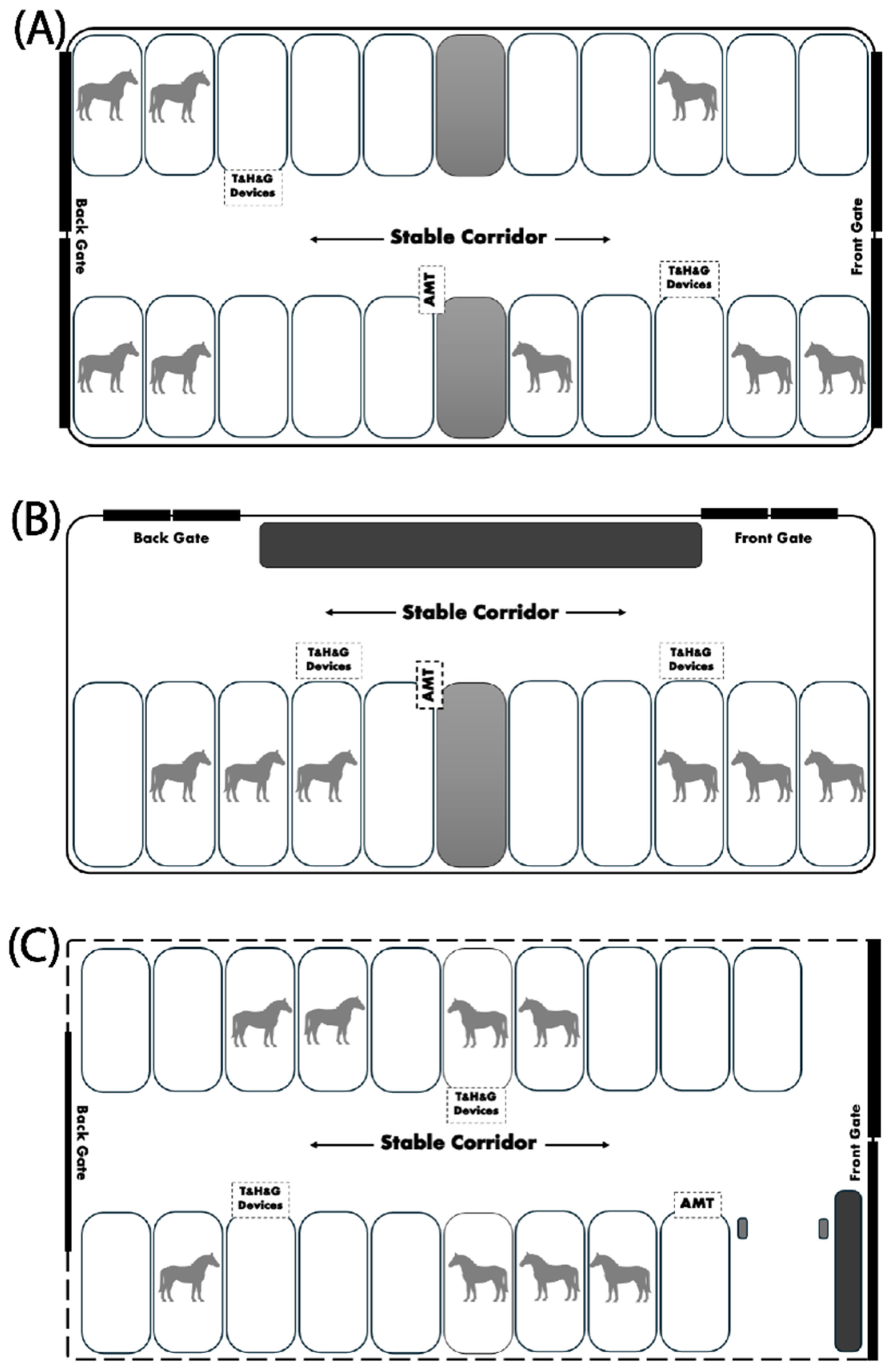
Figure 2.
Air velocity outside and inside different stable architectures during 24 hours of measurement. The air velocity was determined at 07.00 h on the first experiment date until 07.00 h on the consecutive date outside (A) and inside (B) stables. The air velocity was also evaluated during the day and night outside (C) and inside (D) stables. *, **, ***, **** indicate significant differences between comparison pairs at p < 0.05, p < 0.01. p < 0.001, and p < 0.0001, respectively.
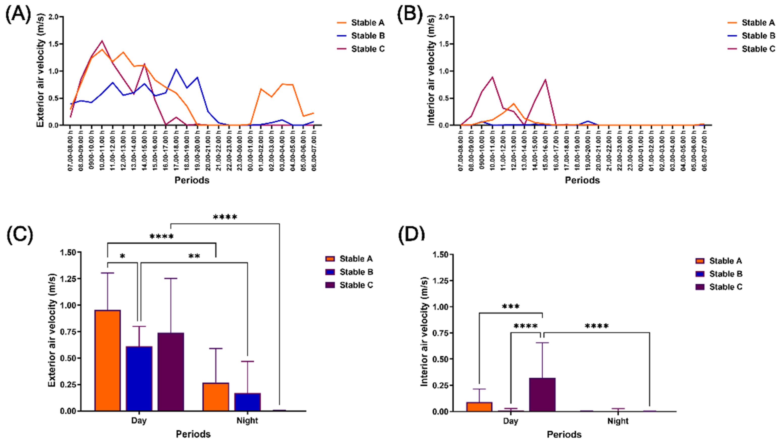
Figure 3.
Relative humidity outside and inside different stable architectures during 24 hours of measurement. Relative humidity was determined at 07.00 h on the first experiment date until 07.00 h on the consecutive date outside (A) and inside (B) stables. The relative humidity was also evaluated during the day and night outside (C) and inside (D) stables. *, **, ***, **** indicate significant difference between comparison pairs at p < 0.05, p < 0.01. p < 0.001 and p < 0.0001, respectively.
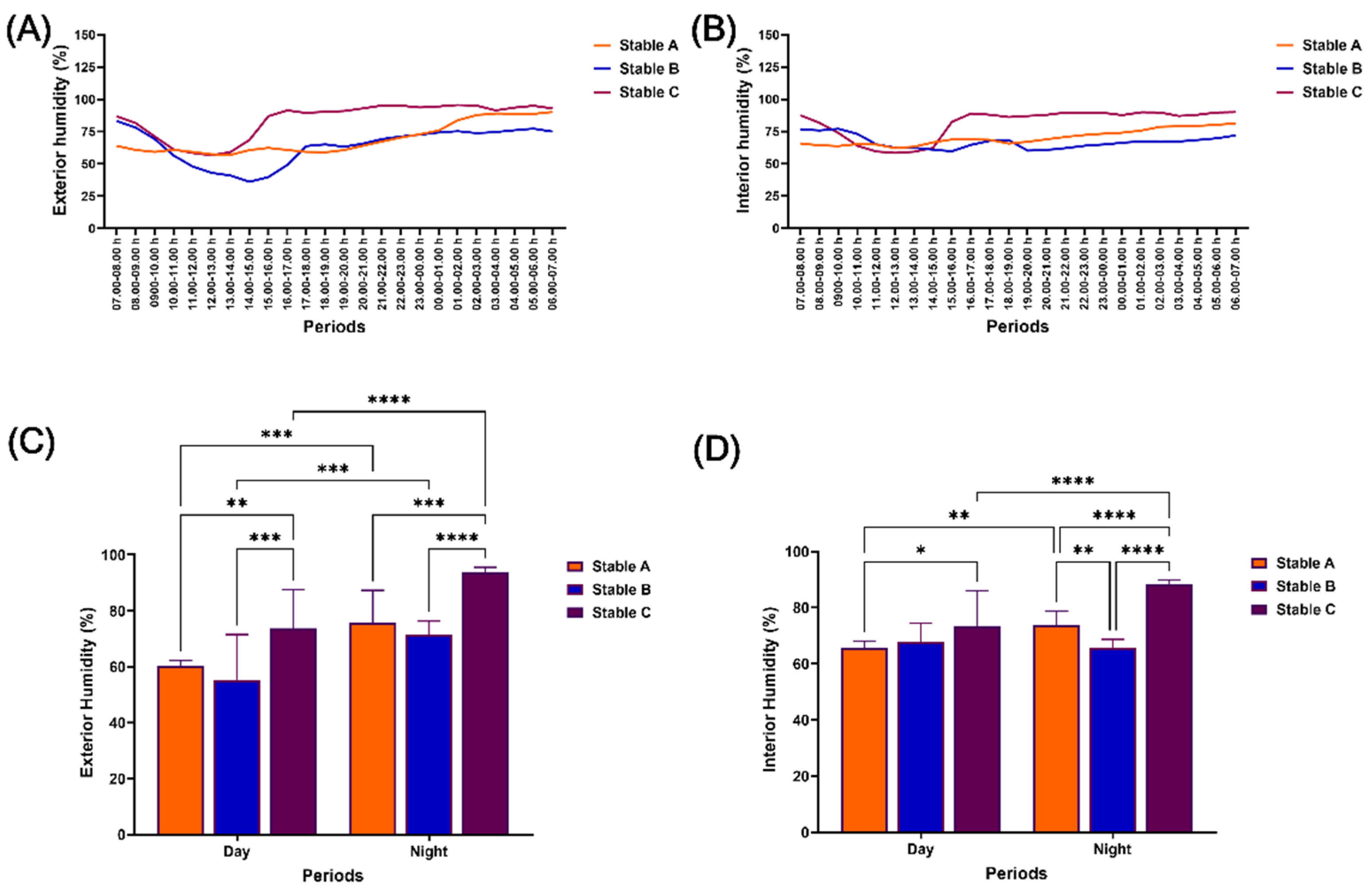
Figure 4.
Air temperature outside and inside different stable architectures during 24–hours of measurement. Air temperature was determined at 07.00 h on the first experiment date until 07.00 h on the consecutive date outside (A) and inside (B) stables. The air temperature was also evaluated day and night outside (C) and inside (D) stables. *, **, ***, **** indicate significant differences between comparison pairs at p < 0.05, p < 0.01, p < 0.001, and p < 0.0001, respectively.
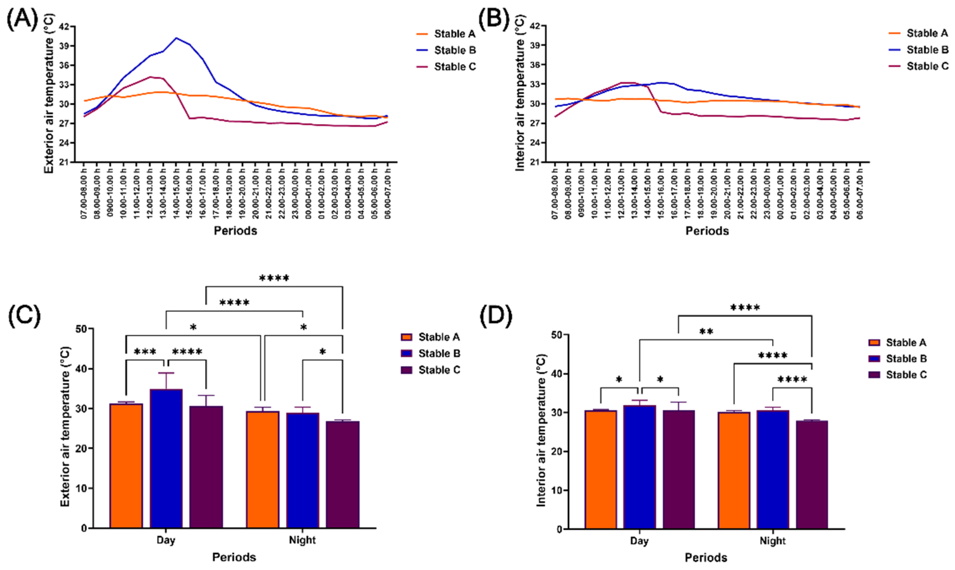
Figure 5.
Ammonia levels within three different stable architectures across the 24-hour cycle (A), during the day (B), and during the night (C).
Figure 5.
Ammonia levels within three different stable architectures across the 24-hour cycle (A), during the day (B), and during the night (C).
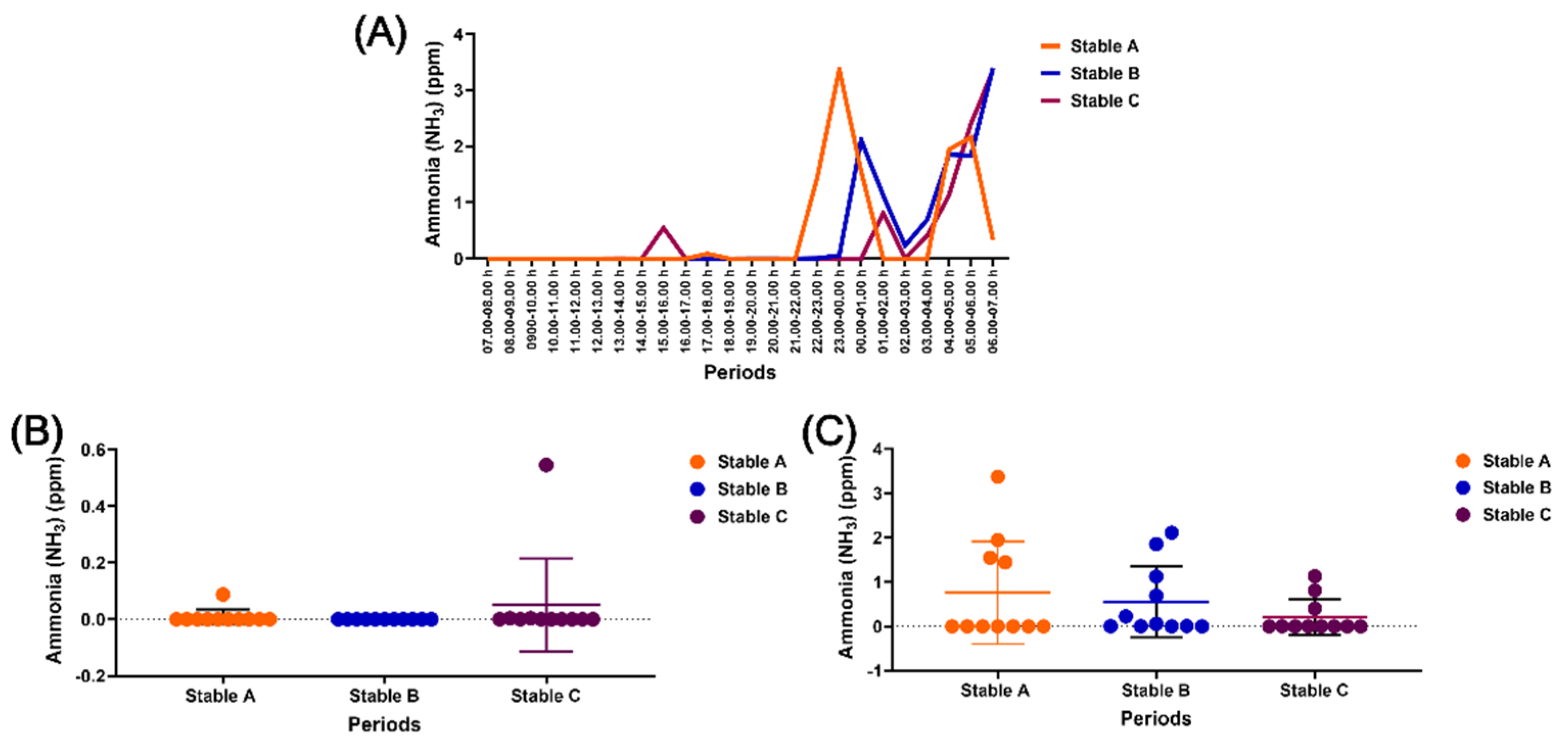
Figure 6.
The impact of housing in three stable architectures on mean beat-to-beat (RR) intervals (A), mean heart rate (HR) (B), parasympathetic nervous system (PNS) index (C), and sympathetic nervous system (SNS) index (D). *, #, and π indicate group-by-time interaction and separate group and time effects, respectively. α, δ, and Ω indicate differences between stables A vs B, A vs C, and B vs C at specific time points. a, b, c, d, e, f, g, h, i, j, k, and l indicate significant differences from the values at 07.00–08.00 h, 08.00–09.00 h, 09.00–10.00 h, 10.00–11.00 h, 11.00–12.00 h, 12.00–13.00 h, 13.00–14.00 h, 14,00–15.00 h, 15.00–16.00 h, 16.00–17.00 h, 17.00–18.00 h, and 18.00–19.00 h, respectively. The indicative letter colours are compatible with those of each matching stable architecture.
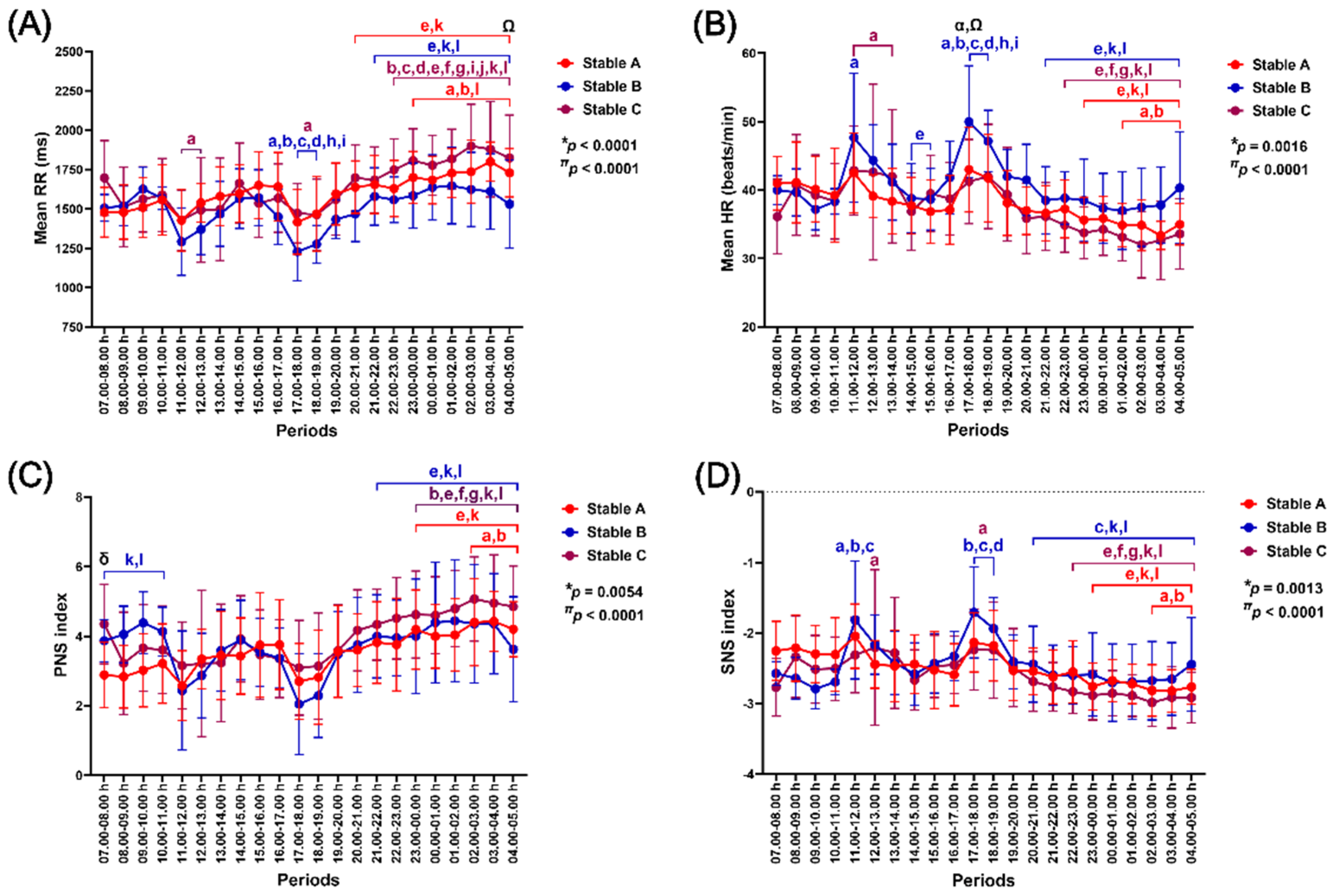
Figure 7.
The impact of housing in three stable architectures on the standard deviations of normal-to-normal RR intervals (SDNN) (A), root mean square of successive RR interval differences (RMSSD) (B), triangular interpolation of normal-to-normal RR intervals (TINN) (C), and the RR triangular index (RRTI) (D). *, #, and π indicate group-by-time interaction and separate group and time effects, respectively. α, δ, and Ω indicate the difference between stables A vs B, A vs C, and B vs C at specific time points. b, h, and i indicate significant differences from the values at 08.00–09.00 h, 14.00–15.00 h, and 15.00–16.00 h, respectively. The indicative letter colours are compatible with those of each matching stable architecture. RR: beat-to-beat intervals.
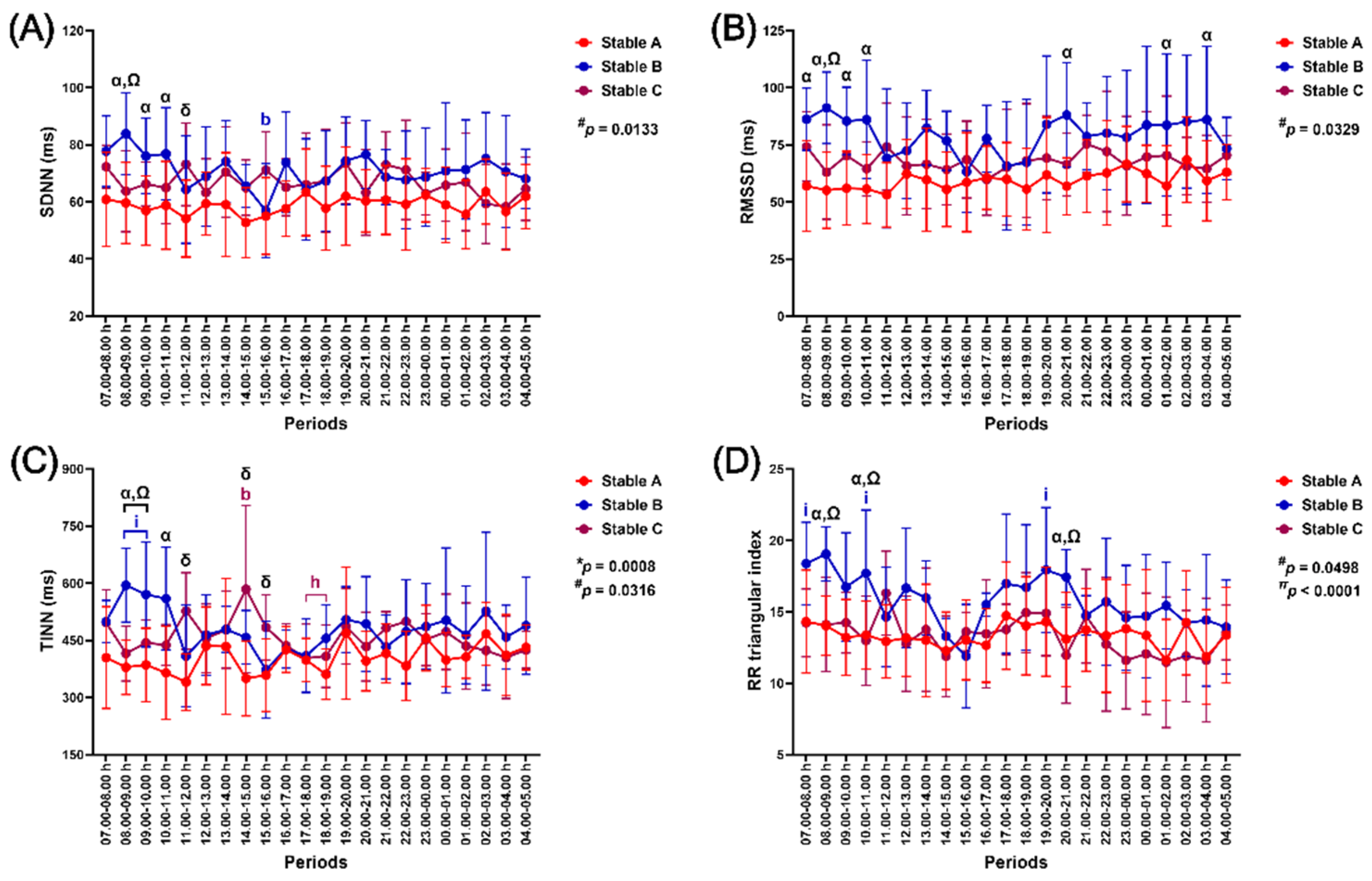
Figure 8.
The impact of housing in three stable architectures on very-low-frequency band (VLF) (A), low-frequency band (LF) (B), high-frequency band (HF) (C), and total power band (D). # and π indicate separate group and time effects. α, δ, and Ω indicate the difference between stables A vs B, A vs C, and B vs C at specific time points. Φ and ϖ indicate significant differences compared to the values at 11.00–12.00 h and 17.00–18.00 h, respectively. b indicates a significant difference from the value at 08.00–09.00 h. The indicative letter colours are compatible with those of each matching stable architecture.
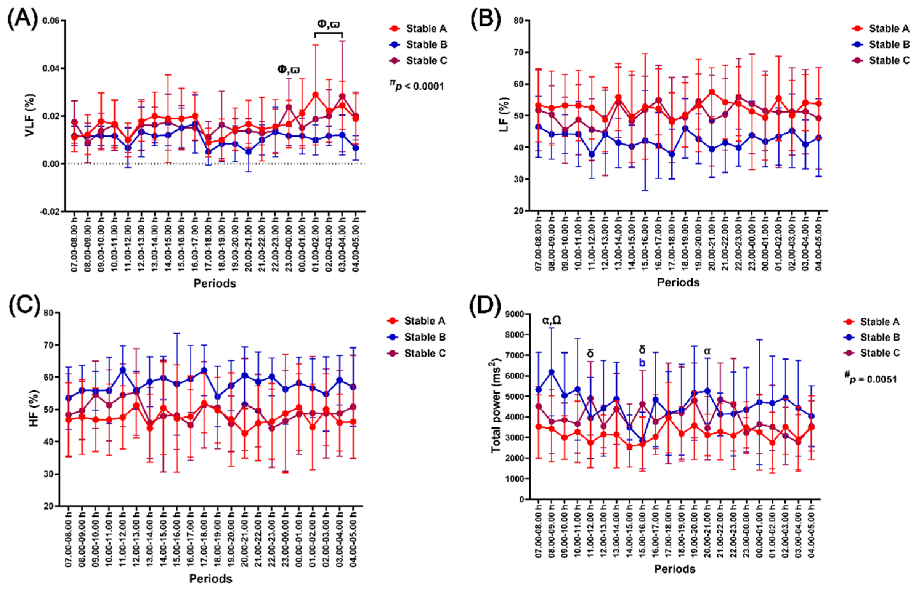
Figure 9.
The impact of housing in three stable architectures on stress index (A), the standard deviation of Poincaré plot perpendicular to the line-of-identity (SD1) (B), the standard deviation of Poincaré plot along the line-of-identity (SD2) (C), and the ratio between SD2 and SD1 (D). *, #, and π indicate the group-by-time interaction and separate group and time effects, respectively. α, δ, and Ω indicate the differences between stables A vs B, A vs C, and B vs C at specific time points. b indicates a significant difference from the value at 08.00–09.00 h. ϖ indicates a significant difference compared to the value at 17.00–18.00 h. The indicative letter colours are compatible with those of each matching stable architecture.
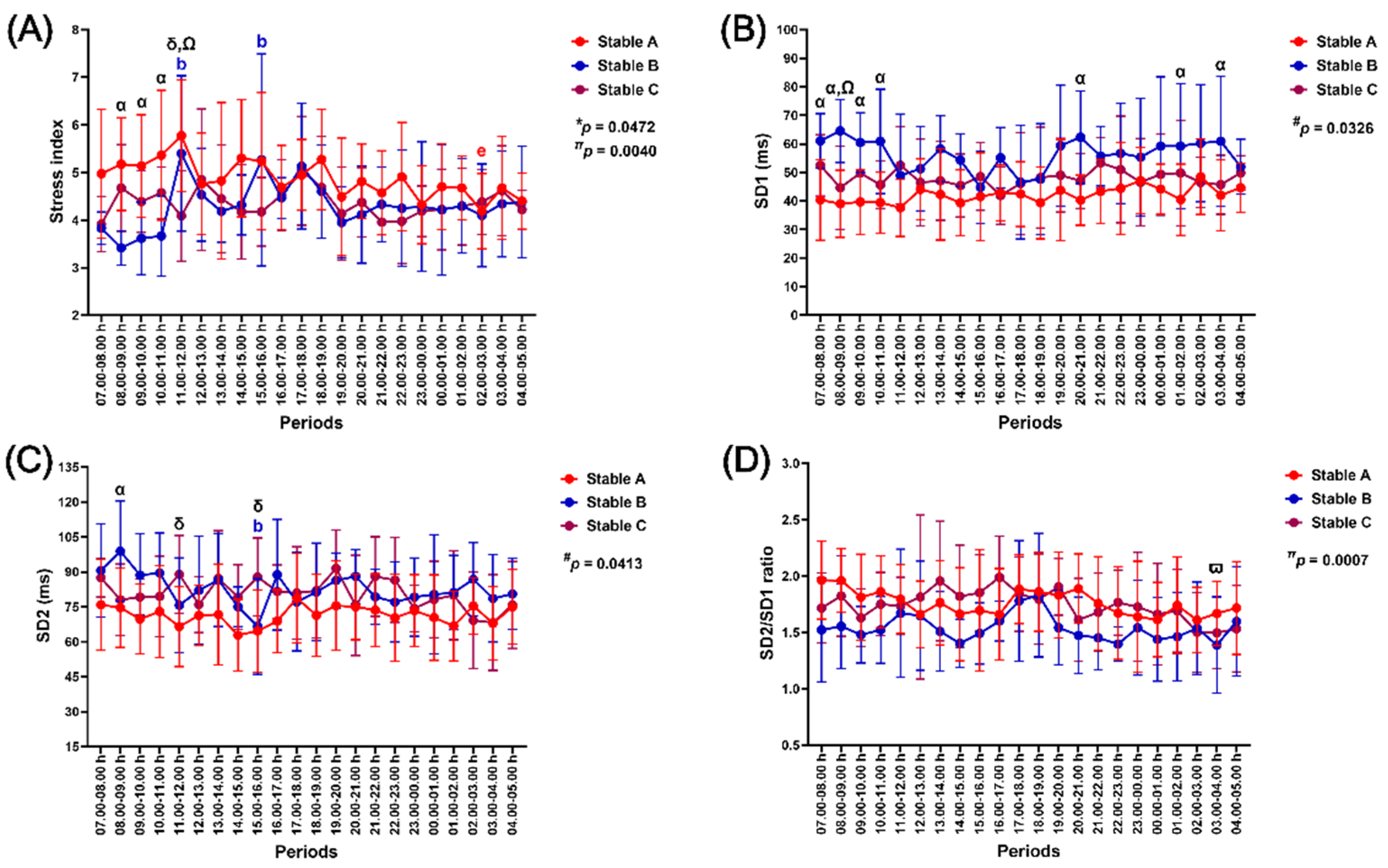
Figure 10.
Correlations between horses’ HRV and microclimate parameters in stable A. The correlation coefficients were determined as representing weak (± 0.10 ≤ rs < ± 0.40), moderate (± 0.40 ≤ rs < ± 0.70), strong (± 0.70 ≤ rs < ± 0.90), or very strong (rs ≥ ± 0.90) correlations. RT: relative humidity, AiT: air temperature, AiV: air velocity, RR: beat-to-beat intervals, HR: heart rate, SDNN: standard deviation of normal-to-normal RR intervals, RMSSD: root mean square of successive differences between RR intervals, TINN: triangular interpolation of normal-to-normal intervals, RRTI: RR triangular index, SI: stress index, VLF: very-low-frequency band, LF: low-frequency band, HF: high-frequency band, SD1: standard deviation of the Poincaré plot perpendicular to the line of identity, SD2: standard deviation of the Poincaré plot along the line of identity, PNS: parasympathetic nervous system, SNS: sympathetic nervous system.
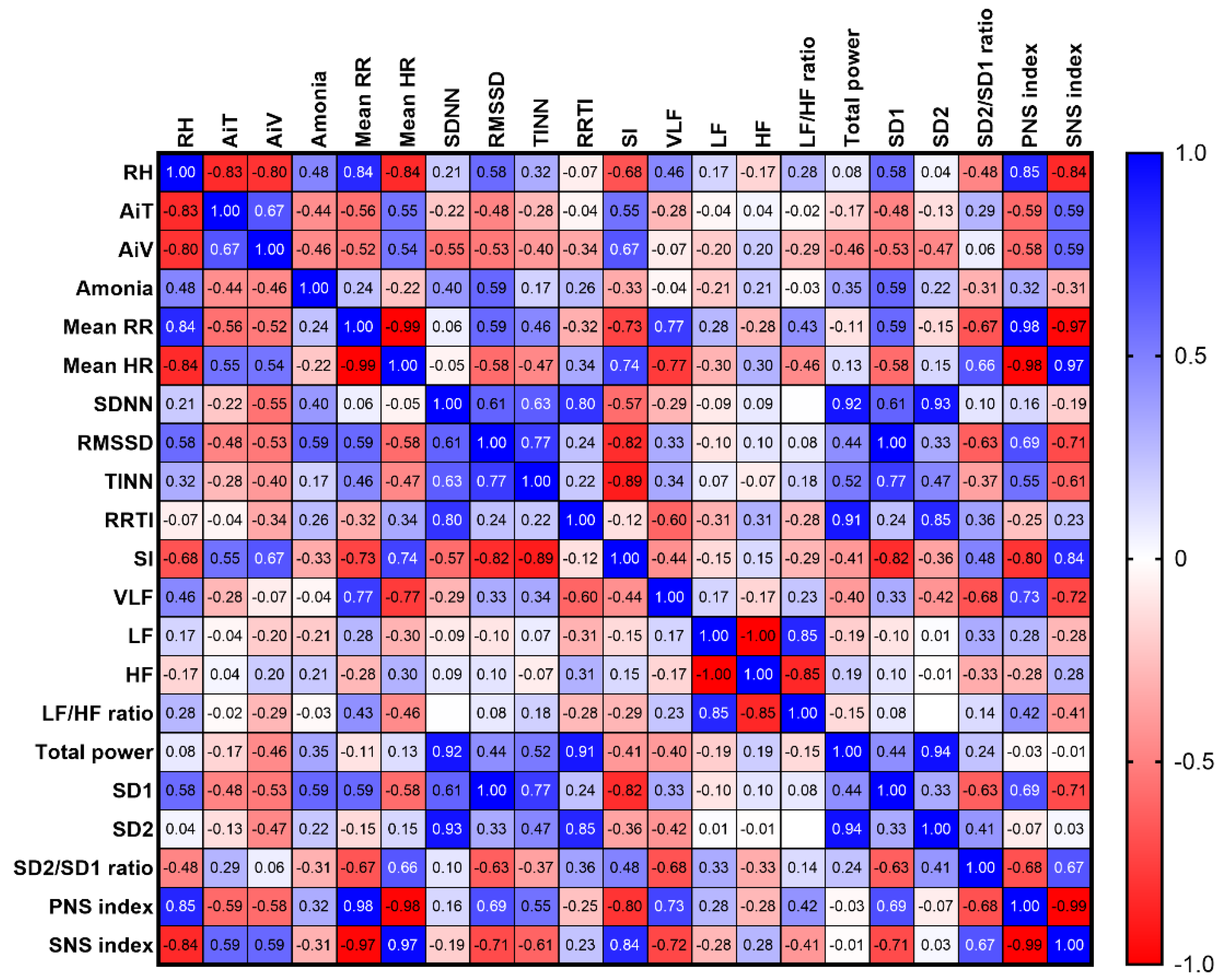
Figure 11.
Correlations between horses’ HRV and microclimate parameters in stable B. The correlation coefficients were determined as representing weak (± 0.10 ≤ rs < ± 0.40), moderate (± 0.40 ≤ rs < ± 0.70), strong (± 0.70 ≤ rs < ± 0.90), or very strong (rs ≥ ± 0.90) correlations. RT: relative humidity, AiT: air temperature, AiV: air velocity, RR: beat-to-beat intervals, HR: heart rate, SDNN: standard deviation of normal-to-normal RR intervals, RMSSD: root mean square of successive differences between RR intervals, TINN: triangular interpolation of normal-to-normal intervals, RRTI: RR triangular index, SI: stress index, VLF: very-low-frequency band, LF: low-frequency band, HF: high-frequency band, SD1: standard deviation of the Poincaré plot perpendicular to the line of identity, SD2: standard deviation of the Poincaré plot along the line of identity, PNS: parasympathetic nervous system, SNS: sympathetic nervous system.
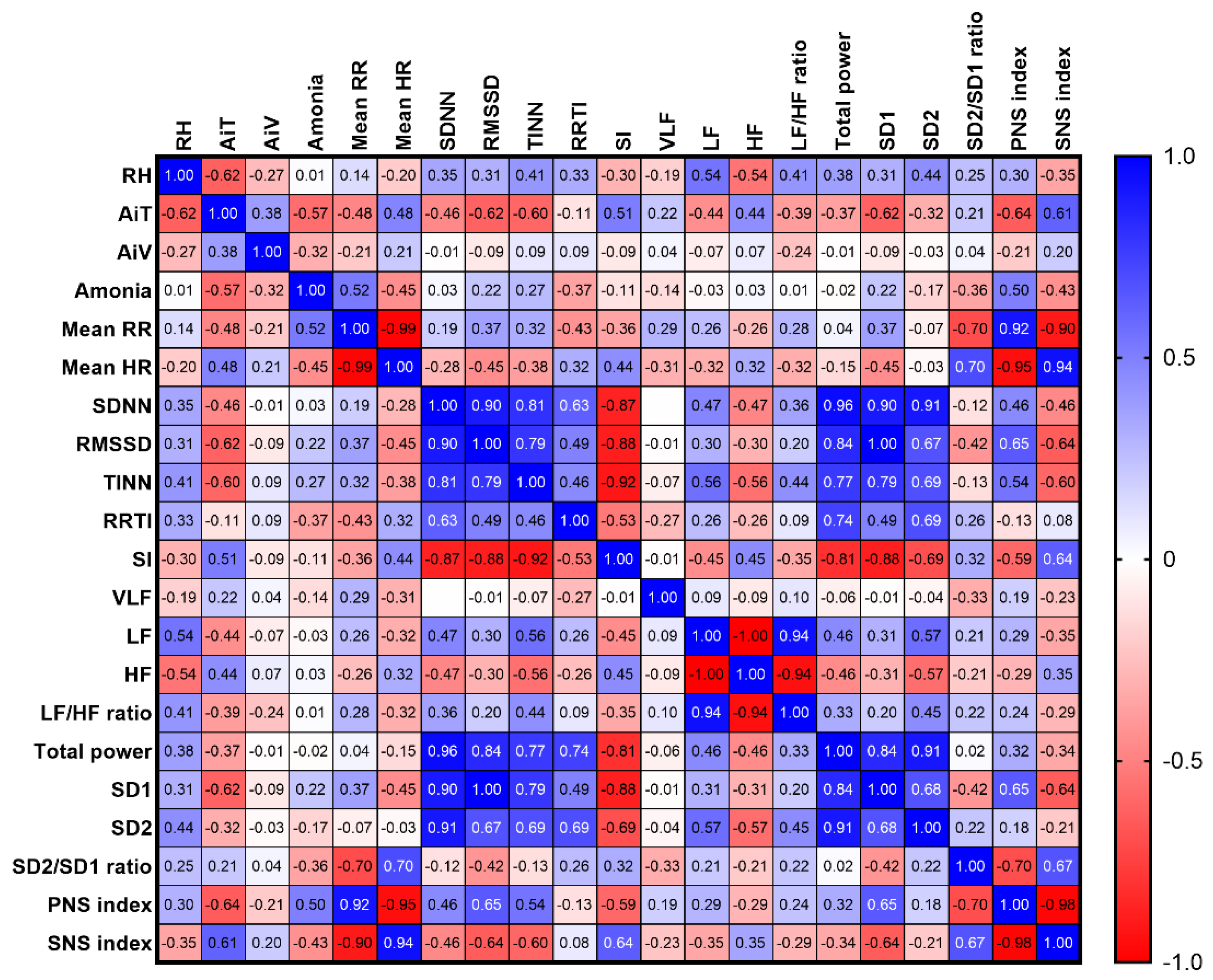
Figure 12.
Correlations between horses’ HRV and microclimate parameters in stable C. The correlation coefficients were determined as representing weak (± 0.10 ≤ rs < ± 0.40), moderate (± 0.40 ≤ rs < ± 0.70), strong (± 0.70 ≤ rs < ± 0.90), or very strong (rs ≥ ± 0.90) correlations. RT: relative humidity, AiT: air temperature, AiV: air velocity, RR: beat-to-beat intervals, HR: heart rate, SDNN: standard deviation of normal-to-normal RR intervals, RMSSD: root mean square of successive differences between RR intervals, TINN: triangular interpolation of normal-to-normal intervals, RRTI: RR triangular index, SI: stress index, VLF: very-low-frequency band, LF: low-frequency band, HF: high-frequency band, SD1: standard deviation of the Poincaré plot perpendicular to the line of identity, SD2: standard deviation of the Poincaré plot along the line of identity, PNS: parasympathetic nervous system, SNS: sympathetic nervous system.
Disclaimer/Publisher’s Note: The statements, opinions and data contained in all publications are solely those of the individual author(s) and contributor(s) and not of MDPI and/or the editor(s). MDPI and/or the editor(s) disclaim responsibility for any injury to people or property resulting from any ideas, methods, instructions or products referred to in the content. |
© 2024 by the authors. Licensee MDPI, Basel, Switzerland. This article is an open access article distributed under the terms and conditions of the Creative Commons Attribution (CC BY) license (http://creativecommons.org/licenses/by/4.0/).
Copyright: This open access article is published under a Creative Commons CC BY 4.0 license, which permit the free download, distribution, and reuse, provided that the author and preprint are cited in any reuse.


