
Submitted:
29 July 2024
Posted:
30 July 2024
You are already at the latest version
Abstract
Solar radiation corresponds to fundamental parameters for solar photovoltaic (PV) technology. Reliable solar radiation prediction became valuable to design solar PV systems, performance, operatively efficient planning, safety operation, grid dispatch and financial characteristics. However, high quality ground-based solar radiation measurements are scarce, especially for very short-term time horizon. Most of the existent studies trained the machine learning (ML) model used dataset with time horizon of 1-hour or day, very fewer studies have been reported using a dataset with a 1-mitute time horizon. In this study, a comprehensive evaluation of nine ensemble learning algorithms (ELA) is performed to estimate the solar radiation in Santo Domingo with a 1-minute time horizon dataset collected from a local weather station. The ensemble learning evaluated included seven homogeneous ensembles; Random Forest (RF), Extra Tree (ET), Adaptive Gradient Boosting (AGB), Gradient Boosting (GB), Extreme Gradient Boosting (XGB), Light Gradient Boosting (LGBM), Histogram-based Gradient Boosting (HGB) and heterogeneous ensemble named as Voting and Stacking. RF, ET, GB, HGB were combined to develop Voting and Stacking and Linear Regression (LR) was adopted in the second layer of the Stacking. Five technical metrics, Mean Squared Error (MSE), Root Mean Squared Error (RMSE), Mean Absolute Error (MAE), Mean Absolute Percentage Error (MAPE) and Coefficient of Determination (R2) were used as criteria to determine the prediction quality of the developed ensemble algorithms. Comparison of the results indicates that the HGB algorithm offers superior prediction performance among the homogeneous ensemble learning and overall, the Stacking provides the best accuracy with metric values of MSE=3218.27, RMSE= 56.73, MAE=29.87, MAPE=10.60, R2=0.964.
Keywords:
ensemble learning
; evaluation metrics
; heterogeneous ensemble learning
; homogeneous ensemble learning
; hyperparameter
; time horizon
; solar radiation
1. Introduction
In the last decade, power generation based on photovoltaic technology has experienced accelerated global growth and will continue with an exponential trend in the next years motivated by several factors 1) new environmental policies to mitigate pollutant emissions generated in the conversion of energy from fossil fuel-based systems [1,2]; 2) tax incentives from local governments; 3) the technological maturity achieved. According to energy statistics solar photovoltaic capacity additions has annually increased on average 15% for the period 2016-2022 and considering a conservative scenario, by 2028 capacity additions is estimated over two times higher compared to values of 2022 [3].
Dominican Republic by the geographical location, presents a favorable scenario for renewable energy expansion driven by the availability of the renewable resource, notably solar and local incentive policies [4,5]. Local actions are implemented to decarbonize the energy matrix. In that sense, the government has established a regulatory framework with the goal of diversifying energy generation systems to include a proportion of 25% renewable energy by 2025, which is equivalent to 2GW based on the current power systems [4,6]. Until now, photovoltaic technology leads in installed capacity compared to other technologies based on renewable resources. Based on that, for the next years, an optimistic scenario is contemplated, marked by an increase in the percentage of solar PV energy penetrating on the grid [4]. However, integrating the power generate by PV systems into the national grid is a complex process that facing many challenges including the lack out of accurate real monitoring and control system, the transportation capacity of the grid, fragile grid infrastructure. The development of robust predictive tools for estimating solar resource based on quality climatic data could contribute to overcome the challenges.
Local climatic conditions are direct correlated to the generation capacity from alternative energies. In specific, solar radiation corresponds to fundamental parameters for solar energy technology. Energy conversion performance of the solar systems is strongly influenced by solar radiation. The transient characteristic of the solar radiation could cause fluctuation on PV energy output and transfer instability to the electrical grid. Consequently, mitigating the variability of the solar radiation on PV energy output and propagation to the grid is essential aspect for maintaining equilibrium and supply quality electricity energy [7,8]. For specific location, the prediction of the available solar resource became valuable to design systems, operatively efficient planning, performance, reduces auxiliary energy storage and financial characteristics.
Access to quality climatic data is a truncated aspect for developing accurate and generalized predictive tool. Dependent on ground-based applications solar radiation is measured with different instruments; pyranometer, pyrheliometer or weather station. In developing countries, quality meteorological data is scarce, mainly motivated by the fact that measurement technologies are limited and cost prohibitive. Robust predictive tools could contribute to solve those constraints, since the tools for predicting can be extrapolated from one location to another.
Several criteria are reported by researchers to classify solar radiation prediction, considering the characteristics of the predictive tools, could be categorized as follows :1) Physical model; 2) Statistic time series; 3) New intelligent tools, 4) Hybrid. Physical models integrate various robust tools, such as approach based on the physical principles governing atmospheric processes (NWP), data assimilation process, satellite, and sky imagen to model atmospheric process. For short-term to long-term time horizons, physical model performance very good prediction ability [9]. The main restriction of the physical models corresponds with computational demand and accessibility to predictor parameters[10]. Statistic tools estimate solar radiation values over a time horizon by statistically analyzing the historical evolution prediction variables. This predictive tool includes several popular techniques, Autoregressive Moving Average (ARMA), Autoregressive Integrated Moving Average (ARIMA). It applied with most frequently to predict short-term horizon, (<6h) and lower requirements for being implemented. In contrast, the predictive capability reduces with increment on time horizon[11].
New intelligence tools referenced to Artificial Intelligence (AI) algorithm categorized by Machine Learning (ML) and Deep Learning (DL). Intelligence tools are becoming more popular motivated by the urgent need to extract productive information from the massive amounts of data generate in a wide range of process. In recent years, specialized scientific community has been developing notably efforts to validate AI algorithms for predicting solar radiation contemplating climatic and geographical parameters at different locations [12]. In early study, report that AI algorithms are suitable to predict solar radiation from short-term to long-term time horizon with a high performance [9,11]. AI algorithms are flexible to numerous types of input parameters and recognizes nonlinear behavioral patterns with great ability. Complicated design code structure and computational time cost are limitation of the AI algorithms [13]. All the AI algorithms are strong function of input data, as consequent, quality data contribute to minimize prediction error. Hence, exploratory analysis and preparation of the database corresponds with essential step to elaborate AI predictive tools. ML regression algorithms commonly studied to evaluate solar radiation include Artificial Neuronal Network (ANN) with single and Multilayer perceptron (MLP-NN), Support Vector Machine (SVM), K-Nearest Neighbors (KNN), Random Forest (RF), Gradient Boosting (GB) while subcategory DL integrate Recurrent Neuronal Network (RNN), Convolutional Neural Network (CNN), Long Short-Term Memory (LSTM). Hybrid predictive tool is based on combination multiple algorithms to enhance the prediction performance, could be combination of physical models with new intelligence tools, or ML with DL and Ensemble Learning (EL), which combines multiple base learner algorithms to obtain robust predictive tool. EL technique can be sorted in homogeneous and heterogeneous ensembles.
The major different between the homogeneous and heterogeneous techniques corresponds to the types of base learner algorithms operative inside the ensemble. Hence, heterogeneous ensemble is based on different learning algorithms while homogeneous used the same type of base learner algorithms to build the ensemble. Homogeneous ensemble could be classified in parallel and sequential by the manner of base learners are trained and combined to perform prediction [14]. In the following lines is presented the literature review focused on research works that used ensemble learning algorithms to capture solar radiation based on historical data measured in diverse geographical locations. In Table 1, summarize the most relevant information of each works
Hassan et al. [15] explored the potential of Bagging (BG), GD, RF, ensemble algorithms to predict solar radiation components for daily and hourly time horizon in the MENA region and compared the prediction performance of ensemble algorithms with SVM, MLP-NN. The database consists in five datasets collected from weather stations located in five countries of the MENA region, during a period from 2010 to 2013.They have not reported the ML techniques employed to clear the data, impute missing values, null exploratory data analysis (EDA) and feature selection. The result indicates that the SVM ML algorithm offers the best combination of stability and prediction accuracy, while it was penalized by computational cost that was 39 times higher in relation to ensemble algorithms. Characteristics of the study is reported in Table 1.
Benali et al. [16] compared the reliability of Smart Persistence, MLP-NN and RF to estimate the Global, Bean and Diffuse solar irradiance at the site of Odeillo (France) for prediction horizon range 1 to 6 hours. The dataset used to perform the study was based on 3 years of data with 10599 observations. They did not develop a full preprocessing and data analysis process. MAE, RMSE, nRMSE, nMAE were the statistical metrics used to evaluate the performance. A relevant finding of this study was that the RF ensemble algorithm predicts the three components of solar radiation with good accuracy.
Park et al. [17] examined the ability of Light Gradient Boosting Machine (LGBM), a homogeneous sequential ensemble algorithm to capture multistep-ahead global solar irradiation for two regions on Jeju Island (South Korea) with time horizon of one (1) hour. In this study, the prediction of the performance of LGBM was compared with two homogeneous ensembles (RF, GB, XGB) and Deep Neural Network (DNN) algorithms using the metric MBE, MAE, RMSE, NRMS. They found that XGB and LGBM methods showed a similar performance and LGBM algorithm ran 17 times faster than XGB.
Lee et al. [18] proposed a comparative study to estimate Global Horizontal Irradiance (GHI) at six different cities of USA using six machine leaning predictive tools; four homogeneous ensemble learning (BG,BS,RF,GRF), SVM and GPR. The database consists of one year of meteorological data by each city. They select the input parameters empirically based on similar study reported literature without considering the algorithms to find the most relevant input parameters. They highlighted that ensemble learning tools were particularly remarkable compared to SVM and GPR. In specific, the GRF tool presented superior metrics to the other ensemble learning.
Kumari and Toshniwal [19] elaborate a homogeneous parallel ensemble based on stacking technique, combining XGB and DNN algorithms to predict hourly GHI by employing a climatic data amassed from 2005 to 2014 at three different locations in India and their result obtained was compared with RF, SVM, XGB and DNN. They concluded that the proposed ensemble reduces the prediction error by 40% in comparison with RF, SVM.
Huang et al. [20] designed research to evaluate the performance of twelve (12) machine learning algorithms in Ganzhou (China) with time horizon corresponding one day and month. The daily dataset was gathered from the period 1980–2016 with a total of 13,100 data point and 432 monthly average points extracted from daily dataset. RMSE, MAE, R2 were used as statistical metrics to compare the capacity of predictive tools. they did not describe the process of combine, clear and filter the data to assembles the database. They found that GB regression algorithms leaded in accuracy over other predictive tools for the daily dataset with R2=0.925, whereas the XGB regression showed the best predictive ability for the monthly datasets obtained R2=0.944.
Al-Ismail et al. [21] carried out a study to compare the predicting capacity of four homogeneous EL algorithms identified as Adaptive Boosting (AdaBoost), Gradient-Boosting (GB), Random Forest (RF), and Bagging (BG) to capture the incident solar irradiation in Bangladesh. The database used was collected from 32 weather stations distribute in separate locations during period 1999 to 2017. In this work were not reported the process to assembly the database, cleaned and filter process. In parallel, dimensionality reduction algorithm was not used. Hence, the preparation stage was incomplete. According to the results GB regression algorithms lead prediction performance compared to other EL algorithms.
Solano and Affonso[22] proposed several heterogeneous ensembles learning predictive tool based on voting average and voting weighted average, combining the following algorithms: RF, XGB, Categorical Boosting (CatBoost), and Adaptive Boosting (AdaBoost) to estimate solar irradiation at Salvador (Brazilian) for time horizon prediction in a range 1 to 12 hours. They used the k-means algorithm to cluster data with similar weather patterns and capture seasonality, while dimensionality of the input parameters was reduced by the output average of the three individual algorithms applied. They result suggest that voting weighted average relating CatBoost and RF offered superior prediction performance compared to the individual algorithms and other ensembles with the following average metrics: MAE of 0.256, RMSE of 0.377, MAPE of 25.659%, and R2 of 0.848.
Based on the literature review, a few studies have been reported that evaluate the predictive performance of the parallel and sequential homogeneous ensemble learning algorithms to capture solar radiation based on historical data measured at single or multiple geographic locations. The following considerations can be drawn from the literature review process:
- In general, “ensemble learning” exhibited superior predictive ability to other individual ML algorithms.
- Most of the previous works studied have not completed or clearly described the ML preprocessing and data analysis stage, which is considered fundamental in the development of ML algorithms.
- A minimal number of the reported articles provided information to the number of points in the collected climate database (Table 1). The number of points in the database is a critical aspect motivated by the fact that the optimal training of ML algorithms is strongly related to the size and quality of the database. In parallel, all the research work has been carried out to estimate the solar radiation considering a prediction horizon greater than or equal to one hour.
- Not studies examined have applied the homogeneous ensemble algorithm identified as Histogram-based Gradient Boosting (HGB) to predict solar radiation.
- None of the manuscripts has proposed a comparative analysis to evaluate the prediction performance of the Voting and Stacking ensemble techniques by combining homogeneous ensemble based on sequential and parallel learning (Table 1).
This research has been designed to contribute to mitigate the limitations found in the literature of solar radiation prediction with new intelligent algorithms. In this sense, a new tool for predicting solar radiation is elaborated based on ensemble learning algorithm using a database for a time horizon of 1-minute, the meteorological measurement is obtained from the weather station located at Santo Domingo de Guzman, Dominican Republic. To do so, firstly, a complete ML preprocessing and analysis stage will be carried out to clean, impute, standardize, and select the subsets of the most relevant input parameters for the development of the prediction tool. Second, the following homogeneous ensemble algorithms will be evaluated: RF, ET, XGB, GB, AGB, HGB, LGBM. Then, homogeneous ensemble algorithms with excellent performance are selected to assemble the heterogeneous Voting and Stacking algorithms. Later, the predictive performance of the Voting and Stacking is compared to determine the predictive tool with superior ability to capture the trend of the test data. MAE, MSE, RMSE, MAPE, R2 were statistical metrics used to evaluate the predictive performance of the ensemble algorithms. The major contribution of this study is described below.
- A comparative analysis will be performed to select the subset of input features that best fit the characteristics of the climate data by employing five ML algorithms to reduce the dimensionality of the database.
- Histogram-based Gradient Boosting (HGB) is adopted for the first time to predict solar irradiance in tropical climates with a time horizon of 1-minute.
- A new tool for solar radiation prediction based on heterogeneous ensemble learning algorithm by combining homogeneous learning with the best performance capability will be proposed.
- The performance prediction of the nine ensemble learning algorithms is evaluated based on metrics MAE, MSE, RMSE, MAPE, R2.
2. Description of Ensemble Learning Algorithms
In recent years, ensemble learning methods have received much attention from the scientific community, mainly motivated by the urgent need to enhance the prediction performance in a wide range of applications such as pattern recognition, natural language processing, medical diagnostics, engineering sciences, energy, environmental sciences, climate forecasting [23].
An ensemble combines a number of trained base learners to generate a single learner with a superior generalization ability to solve problems effectively with minimal prediction errors. Two fundamental characteristics of the ensemble methods are the diversity of the ensemble and aggregation of the base learners [14]. Ensemble learning can be divided into two subcategories; 1) homogeneous ensembles use the same type of base learners 2) heterogeneous ensembles are created with different type of base learners. Homogeneous ensembles can be subdivided into sequential or parallel, commonly denote to Boosting and Bootstrap aggregating (Bagging), respectively. Figure 1 illustrates the general architecture of ensemble learning algorithms, as can be noted, the main different between homogeneous sequential and parallel is based on the manner in which the training dataset is manipulated during the training process of the base learners. In the parallel ensembles, the original training set is resampled to generate new subsets of training data.
Thus, multiple base learning algorithms of the same type are trained separately with the generated subsets. Then, the outputs of the base learners are aggregated to calculate overall prediction values (Figure 1). In the sequential ensembles, the training process of base learners is carried out iteratively, base learner depends on the information provided by the previous learners, as consequence, base learners learn from the errors of previous iterations by increasing the importance of those incorrectly predicted training instances in future iterations [24].
2.1. Parallel Homogeneous Ensemble
2.1.1. Random Forest (RF)
RF Was introduced by Breiman [25], since then, it has become in one of the most widely used ensemble learning methods for classification and regression tree ML problems. This is probably because RF work with efficiency and relative simplicity. RF use randomized decision trees as base learners, where each decision tree is trained with a different training set resulting from random resampling with replacement of the original dataset. For regression ML problems, the output of an RF prediction is calculated by averaging the output predictions associated with each randomized decision tree. the RF ensemble has numerous advantages, provides a ranking with the level of importance of the variables in the process, reduce problem with overfitting, not affecting by outliers observations, can be parallelized for fast implementation, small dimension of hyperparameters space. In contract, consumes computing resources with many trees and a large database. A rigorous explanation of RF fundament is found[26].
2.1.2. Extremely Randomized Trees (ET)
Modified algorithm of RF presented by Geurts et al. [27], differ with RF in various aspects; Firstly, the level of randomness, ET goes further and became the process completely random; generating training sets from original data random and without replacement, also randomizing both attribute selection and threshold determination. Second, the computer time cost of ET is minus that the RF. In a Ref.[28] reported that ET is appropriated to work with large datasets while for small dataset could be disposed to overfitting.
2.2. Sequential Homogeneous Ensemble
In the last years, several ensemble methods based on sequential technique have been proposed. The core of any sequential ensembles is the boosting algorithm, so the new tools modified or introduce innovations to the boosting algorithm. In the following lines, a brief description of the main characteristics of the sequential ensembles adopted for this work is presented.
2.2.1. Adaptive Boosting (AB)
AB was developed by Freund and Schapire [29]. The algorithm was first introduced to ML classified and then for ML regression problems. AB differ from Boosting in several aspects 1) The base learner is forced to focus on the weights of incorrectly classified instances in the training set.2) The final prediction of AB is obtained by combine all the base learners results through the rule of weighted majority voting. it is widely adopted since fast implementation, simplicity structure, reduce number of hyperparameters and good compatibility [26]. Possible disadvantages for the algorithm, it is very sensitive to noise and the predictive capacity of the AB deteriorates with scarce data.
2.2.2. Gradient Boosting (GB)
Was proposed by Friedman in series of studies and function as general framework uses decision trees as base learners [30,31]. The GB Decision Trees is very important ensemble algorithm motivated by the fact that is the based line of the new gradient algorithms; XGBM, LGBM, Categorical Boosting (CatBoot). Like as AB applies the sequential ensemble principle. However, the GB focuses on working with large errors resulting from the previous iterations. The GB is based on gradient descent optimization algorithm to minimize the loss function while enhances the prediction performance.
The learning process is iterative, the GB generates a series of base learners. The first base learner is training with the original dataset to make predictions and produce residual error, then the actual base learner is training with the residuals of its predecessor. A solution of the process is archives when convergence to minimum error value by following the direction of the negative gradient resulting in a perform robust future prediction. The main components of the GB algorithm could be classified; 1) based learner, typical decision trees algorithm; 2) Loss function; 3) regularization. GB Decision Trees is a strong ensemble algorithm with ability to high prediction performance, capture complex patterns in the data, work better for low-dimensional data, could tend to overfitting with noisy data [32]. A deep explanation of statistics fundamental of Gradient Boosting algorithm could be found in reference [33].
2.2.3. Extreme Gradient Boosting (XGB)
Updated the GB decision tree algorithm to optimize the tree structure and implemented regularizations into the loss function to control overfitting. The XGB such as the RF and ET algorithms could be parallelized, the result is a faster learning procedure which allows quicker exploration. It was first introduced in 2016 [34]. Since then, it has been applied to solve many prediction problems in different fields; finance, healthcare, e-comerce, and so on.
2.2.4. LightGBM (LGBM)
It is another efficient gradient boosting decision tree framework proposed by Microsoft collaborators [35] to work with large dataset, based on the primacy that the computational efficiency and scalability for GB, XGB algorithms needed to be improved. The LGBM introduces several novel advances to GB algorithms: uses histogram-based splitting algorithms, which bucket continuous attribute values into discrete bins; leaf-wise tree growth with deep limitation; sample weighting Gradient-Based One-Side Sampling (GOSS) and Exclusive Feature Bundling (EFB). According to the authors, all these improvements result in the following advantages: faster training process, lower computational cost, ability to work with large-scale datasets, and better accuracy.
2.2.5. Histogram-Based Gradient Boosting (HGB)
Recently, Scikit-Learn proposed a version of Histogram-based Gradient Boosting decision Trees [36,37]. According to them, the algorithm is based on a modern gradient boosting implementation comparable to LGBM or XGB. Their HGB algorithm offer several advantages with regarding to GB, make it interesting tool to predictive modelling. Several available loss functions, early stopping to prevent overfitting, missing values support, which avoids the need for an imputer. Faster training process with dataset higher than 10,000 points.
2.3. Heterogeneous Ensemble Learning
2.3.1. Voting
It is a heterogeneous ensemble learning method that aggregates the output predictions of the multiple models to improve the overall prediction performance. Voting is considered a meta-learner since it trains several base learners, each one with the complete dataset, and then it integrates the predictions of the learners using an averaging approach to obtain a final output. Voting can be classified by the manner of the predictions are combined; 1) majority voting; 2) simple average voting, where the final prediction is calculated with the average value of the prediction results of the individual base learners; 3) weighted average voting, in this case, the overall prediction is estimated with the weighted arithmetic mean, assigning different weights to the base learners depending on their individual performance.
2.3.2. Stacked Generalization.
Classified as a superior heterogeneous ensemble learning, which uses aggregation techniques to combine multiple base learners in a two-layers structure [38]. In the first layer, several base learners are trained in parallel, each one with the same training set, and the resulting predictions of the base learners become a new output dataset. In the second layer, the output dataset of the first layer is used as input to train a second level ML algorithm, which is labeled as the meta learner Then, the final prediction is the output of the second level ML algorithm. Practical evidence [39] shows that training simple ML algorithm (linear regression) instead of a complex model in the second layer could prevent overfitting problems.
3. Materials and Methods
The methodology proposed for the development work consists of a computational simulation for modeling ensemble ML algorithms based on historical climate data. Python programming language, supported by the following open libraries: NumPy, Pandas, Searbon, scikit-learn, XGBoost and LightGBM has been used to perform the simulations. Table 2 describes the computational resources used for the simulation implementation.
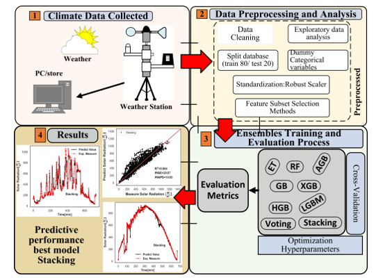
The proposed workflow is shown in Figure 2. As can be seen, first, a database was collected based on measurements of the local meteorological parameters by means of local weather station. Second, preprocessing and analysis is applied to the database. then, trained process to find appropriate values of hyperparameters. Finally, evaluation based on technical metrics and analysis of the results is performance.
3.1. Data Collection
The study site is located at the city of Santo Domingo, National District of the Dominican Republic, a Caribbean Sea country. Santo Domingo is characterized by a tropical savanna climate with average annual values; minimum /maximum temperatures in the range 22°C-28°C, an annual rainfall 1,380 millimeters and a relative humidity around 85% [40]. For the city of Santo Domingo, according to the research in Refs[41], the average values of Global Horizontal Irradiation (GHI) vary in the range of 5.2-5.6 kWh/m2/day and the annual average daily sunshine is 8.6 hours. A Dominican Republic map with information on the average values of GHI for the period 1999-2018, is shown in the Figure 3.
The weather station, model Vantage Pro2 Plus (Davis Instruments) was installed on the roof of the Faculty of Health Sciences and Engineering (FCSI) building of the Pontificia Universidad Católica Madre y Maestra (PUCMM) at latitude 18°27’46.59”N, longitude 69°55’47.60”W and an elevation of 50 meters above sea level. The Weather station is illustrated in Figure 4.
Vantage Pro2 Plus weather station is equipped with Integration Sensor Suit (ISS) to convert the meteorological parameters to output electrical signal and a console for real time monitoring, internal operation, and data logger. Table 3 shows the characteristics of the measured meteorological parameters by the weather station. A wide range of parameters can be measured by Integration Sensor Suit of the Vantage Pro2 Plus: temperatures, barometric pressure, wind direction-speed, solar radiation, UV solar radiation, rainfall levels, relative humidity, dew point and it can calculate new index based on the combination of measured parameters: THW, THSW, Heat index, Wind Chill. At the same time, the minimum and maximum values of meteorological parameters for certain periods of time can be provided by the console. Additionally, the console incorporates internal sensors to measure temperature, humidity, and derivative parameters at the location where it is mounted. It is worth to mentioning that the integration sensor suit acquired did not include the UV sensor. Therefore, the UV index was not considered in this study. The console was configured to record meteorological parameters every minute and the data were transferred to the computer unit via software interface (WeatherLink). The database was created by integrating all meteorological measurements during the period January-May, year 2022. The dimension of the database without preprocessing corresponds to 170,861 observations and 35 attributes.
3.2. Data Preprocessing and Analysis
The data preprocessing and analysis stage is fundamental to the development of robust ML algorithms. To carry out this stage, the raw database was first submitted to a careful cleaning process, in which, the measurements with solar irradiance values lower than 5 W/m2 (at night hours, low solar altitudes) were eliminated by applying a filter to consider only the sunlight available from 7:30 a.m. to 6:30 p.m. After selecting the daily sample range, the few missing values present in the database (0.008% of the data) were replaced one by one with new values using imputation algorithms. The following strategies were executed for the imputation process: the missing values data located in the categorical parameters were filled with the most frequent values by applying the univariate algorithm, while for the numerical parameters the nearest neighbor algorithm was adopted to replace each missing value by a new one. As a result of the cleaning process, a new dataset is created with a daily sample of 11 hours and a dimension of 78,536 observations and 35 attributes (about 54.1% of the data were not used).
Exploratory data analysis (EDA) was conducted to examine the characteristics of the dataset resulting from the cleaning process. In general, the wind blows from the north(N), northeast (NE), north-northeast (NNE) directions with the average wind speed of 2.18 m/s and the average outdoor air temperature of 26.93 Celsius and relative humidity 76%. Solar radiation computed an average value 436.85 W/m2, a maximum value 1211 W/m2 and a minimum value of 5 W/m2, most values of the solar radiation were collected in the north cardinal point of the wind direction, as can be seen in Figure 5a-b. North and northeast wind directions grouped the solar radiation values with the highest and lowest variability, respectively (Figure 5a). In Figure 5a can be noted that the median and interquartile range of solar radiation exhibited similar values in the north-northeast and northeast directions, while the northeast wind direction is the most compact distribution.
For possible outlier values, the interquartile range technique was applied to all parameters in the dataset, as results of process not outlier values were found. As can be observed in Figure 5a-b, wind direction (WD) and high wind direction (HD) parameters shown a certain degree of variability on solar radiation, to study the propagation effects on solar radiation, the dummy ML technique was used to convert them into numerical values and visualize the contribution to the objective variable on coefficient matrix.
Distribution of solar radiation by wind directions for the range of the daily sun hours sample is shown in Figure 6c. As can be noticed, a line is connected the maximum radiation values for each hour resulting in a representation of figure merit for behavior solar radiation. Approximately 75.67% of the solar radiation measurements were captured when the wind was blowing from the north(N) direction, 23.75% correspond to the north-northeast (NNE) wind direction and only 0.09% were taken in the northeast (NE) wind direction. The solar radiation observations are distributed by hours as follows; 55% of the solar radiation values are scattered in the time range 10:30 a.m.-4:30 p.m. (from 4 to 9 hours) and 18% of the solar radiation points were captured by the first and last hours of the daily solar sample. Average values of solar radiation by daily sun hours are shown on Figure 6d. The tendency of the figure indicate that the maximum average value of the solar radiation was obtained from 12:30 p.m. to 1:30 p.m. (the 6th hour of the daily solar sample) with a value of 676.45 W/m2, while a minimum value is obtained at sunset hour (the 11th hour of the daily solar sample, 5:30 p.m-6:30 p.m.).
A heat map of the matrix correlation based on the Pearson coefficient (Figure 7) was elaborated for a preliminary examination of the interaction of the input parameters with the solar radiation. The following considerations were found:
- Arc.Int and Heat D-D parameters were eliminated of the dataset, since reported constant values (not variability).
- In the Pearson correlation matrix, pairs of correlated input predictors parameters can be identified based on correlation coefficient values higher 0.8 and lower -0.8 (collinearity); Wind Chill, Heat Index, THW index , Cool D-D are each separately correlated with Temp Out. Wind Run is associated with Wind speed; In EMC is related to In Hum. In Hum and In Temp are correlated, as well as In Dew with Dew Pt.. Rain is correlated to Rain rate. In parallel, there is a strong linear correlation between many measured meteorological parameters and the High (Hi)- Low (Low) registered values corresponding to each one of the parameters. This effect could be due to the fact that a very short time has been set for updating the DAQ lecture (1-minute/lecture). Therefore, for many parameters, the measured values and high-low register values do not differ. As a consequence, the following input predictor parameters were deleted from the dataset to prevent a propagation effect of the collinearity in the process of subset feature selection and possible bias in the technical evaluation metrics: Wind Chill, Heat Index, THW index , Cool D-D, Wind speed, In EMC, In Hum, In Dew, Rain rate, Hi Temp, Low Temp, Hi speed, Hi solar Rad. (store high and low values);
- Wind direction (Wind Dir) and high wind direction (Hi Dir) parameters could have some influence on solar radiation based on Figure 5a-b. Therefore, they were converted to numerical values by dummy technique and included intro the matrix correlation labels as WD_N, WD_NE, WD_NNE, HD_N, HD_NE, HD_NNE. In Figure 7 can be seen WD_NNE, HD_N has effect on solar radiation.
- Solar Energy parameter is computed from solar Radiation, so its collinearity is structural. As consequent, Solar Energy was not included in the dataset using to the feature selection process.
After applying the aforementioned considerations to remove the input predictor parameters, the dimensionality of the dataset is reduced, as a result, a new dataset is generated with 78,536 rows and 20 columns. The Figure 8, show the degree of the strength for the correlation between input parameters of the new dataset and solar radiation.
3.3. Splitting the Dataset
The strategy used to stratify the dataset is crucial to evaluate the ML prediction tools and achieve excellent results. Based on the chronological characteristics of the dataset, the time series cross-validation stratified split strategy was considered to divide the dataset into train and test sets with a proportion of 80:20. As a result of the splitting process, the training set consisted of 62,829 observations while the test set consisted of 15,707 observations, both train/test sets have 20 attributes. This stratification strategy ensures that the training process of the predictive tools is carried out on the chronologically historical dataset and the performance is evaluated on the future dataset. The normal strategy of shuffling and randomly stratifying the dataset is not suitable in this study, motivated by the fact that the ML predictive tools could learn from the future behavior of the unseen data during the training process, thus improving the technical evaluation metrics, but this is not a realistic scenario.
3.4. Standardization of the Dataset
The standardization technique identified as Robust Scaler was applied to the dataset to transform the input variables to a specific scale range with similar distribution. The Robust Scaler associated the median and interquartile range to scale the measurement of each input variable, is given by the following equation.
Where is the interquartile range for the input variable, median value for the measurements of each input variable, , is the measure values, , new values scaler with Robust technique. The robust scaler has been considered to standardize the dataset motivated by the fact that it is not affected by outlier observations, which could result in an advantage for working with aleatory-chaotic characteristic of the weather conditions.
3.5. Feature Selection
ML models are very sensitive to the input variables, so selecting a relevant subset of input variables improves the predictive ability of the model. After the cleaning and exploration process, the dataset has a dimension of 78,536 observations x 20 attributes. Therefore, it has many variables that may cause noise or may not propagate their effect to the objective variable. Under these characteristics, it is necessary to reduce the dimensionality of the future space to obtain a new smaller dataset without penalizing the predictive performance of the ML algorithms. Feature subset selection contributes to better interpretability of input features, prevents overfitting, improves generalization capacity of ML algorithms. There are several methods in the literature to reduce the dimensionality of the dataset.
In this study, a comparative analysis was carried out considering five feature subset selection methods with the objective to determine the appropriate subset of input features. For this purpose, the first step was to obtain a subset of features (input variables) generated by each of the feature selection methods. Then, each subset of features was implemented to fit through the training set five ensemble learning algorithms using the default values of the hyperparameters. Finally, the predictive performance of each ensemble learning was evaluated by the coefficient of determination (R2) with the test set portion order to examine which of the five subsets of features lead the performance based on the coefficient of determination score. Results of the comparison for the five feature selection methods is reported in Table 4.
3.5.1. The Pearson Coefficient
The following is a brief description of the selection feature methods adopted to select an appropriate subset of input features was the first methods used to select a subset relevant input feature. Figure 9a shows the relationship between the input feature and solar radiation with a filter to consider only coefficient values higher than 0.1 and lower than -0.1 applying these filters was obtained a subset of eight input parameters (Table 4).
3.5.2. Recursive Feature Elimination (RFE)
Method was adopted with RF as external ML algorithms. The main propose of the RFE is to create a subset of features by recursively eliminating the least important features. The ranking generated by the algorithm from the most important feature to the least important feature is shown in Figure 9b.
3.5.3. SelectKBest(SKBest)
It is a univariate feature selection method in the scikit-learn library that examines each feature individually to determine and select features based on the highest results on the objective variable. Configuration and evaluation of the ensemble learning algorithms with subset of features generated by SelectKBest methods are reported in Table 4.
3.5.4. Sequential Future Selection (SFS)
Wrapper methods based on iterative approach reduces the dimensionality of the dataset prioritize features with highest evaluation metric to create a subset of features that strongly influence the objective variables. SFS have two iterative directions technique can be classified as forward and backward. The main difference between forward and backward schemes is the direction of the iterative process. In forward, the ML selection algorithms begin without features and in each iteration adds a feature one by one, choosing the one with the most predictive ability. In backward, begin with all features of the dataset and in each iteration remove features one by one, until obtaining new smaller subset whose the performance prediction enhance. Results of both SFS technique is reported in Table 4.
The subset of features obtained with the selection method RFE adopting RF regressor as external ML algorithms lead the other selection feature methods with slightly better score for each ensemble learning tested (Table 4).
Therefore, the subset of features selected to perform the training and evaluation process of the ensemble learning models corresponds to the follow features; {In Temp, In Density, Out Hum, Bar, THSW Index, Wind Speed, Dew Pt., Temp Out}, count with eight features. As a result of the subset feature selection process, a new reduced dataset with a dimension of 78,536 observations x 8 attributes was generated.
The distribution curve of the selected subset of input features standardized by Robust Scaler technique (Eq.1) is shown Figure 10, as can be noted, the eight features are scaled at the same range and the distribution is very similar make an equal contribution of each feature
3.6. Training Process
The training procedure is a critical stage in the ML methodology, since in this procedure it is required to find a set of hyperparameters that maximize the predictive performance and minimize the general expect loss of the ML algorithms. Currently, several optimization strategies can be identified in the literature to find an appropriate hyperparameter configuration for an ML algorithm trained on a dataset [43]. A necessary step in the hyperparameter tuning process consists to the cross-validation (CV), which is a statistical technique to evaluate the accuracy of ML algorithms during the training process. CV iteratively partitioning the dataset into training and testing portions, training the ML algorithm on some of these portions, and evaluating it on the remaining test portion.
In this work, the optimization strategy was established based on a random search of the hyperparameters combined with a CV. Random search is an optimization technique that implements random sampling over a predefined search space to find a set of appropriate hyperparameter values and evaluates the performance of ML algorithms using cross-validation over the training dataset. The hyperparameter tuning process for all the ensemble learning algorithms studied was performed using the RandomizedSearchCV tool available on the open source Scikit-Learn Python Library. The way to use RandomizedSearchCV can be described as the following steps: 1) Training set well defined; 2) The ensemble learning algorithms using for hyperparameter optimization; 3) Create the hyperparameters space to search and find best values; 4) CV strategy applied on the training set; 5) Set the depth of the exploration to search in the hyperparameter space; 6) metric to score the accuracy of the training ML models. The corresponding hyperparameter values for each tuning ensemble and the computational cost for the training process can be seen in Table 5.
The hyperparameter search space was elaborated based on the structure of each ensemble algorithm, and the seed values for each of the hyperparameters were assigned empirically. Coefficient of determination (R2) was using during the hyperparameter tuning process as metric to score and select the ensemble with best overall score results. For cross-validation, the KFold cross-validation strategy was adopted with fixed five folds (K=5) without shuffling the training set, because the dataset corresponds to a historical series, therefore, unseen or future data could be filtered out. During the cross-validation process, the training dataset (80% of the data) is partitioned into five folds (portions). In each fold, the ML ensemble learning is trained using four folds and one-fold is retained as a test set to evaluate the accuracy, the training and testing sets change across each fold. The final score is obtained by calculate the average of the five folds. Regarding the depth of the exploration to search in the hyperparameter space, which represents the number of iterations to explore the predefined space of hyperparameters. It is a very complex parameter and to the best of the authors knowledge, until to now, no rule has yet been reported to define it. Therefore, as an alternative, it could be defined empirically considering the size of the hyperparameter space and the available computing capacity. Set values of iterations and number of cores used for each ensemble learning are reported in Table 5.
3.7. Evaluation Metrics
Predictive efficiency in the performance of ML algorithms is quantified by statistical metrics that indicate the degree of deviation of the predicted values from the real values. In basic terms, how close the predicted outcomes of the model are to the real values. In this work, five statistical metrics were used to evaluate the predictive ability of each ensemble learning algorithm trained to approximate the real values of solar radiation measurements: Mean Squared Error (MSE, Eq.2), Root Mean squared Error (RMSE, Eq.3), Mean Absolute Error (MAE, Eq.4), Mean absolute percentage Error (MAPE, Eq.5), Coefficient of Determination (R2, Eq.6) . Several metrics were selected to examine very well the error generated when comparing the ensemble learning prediction results with the real measured value
Where is the measurement value of the solar radiation, predicted value of the solar radiation, is the residual sum of squares calculated by the sum of the squares of the differences between the measured solar radiation value and the predicted values while corresponds to the total sum of squares. is the number of observations (measured values) in dataset.
4. Discussion and Results
A database was created by integrating meteorological parameters measured with a time horizon of 1 min from January to May using a weather station located at latitude 18°27’46.59”N, longitude 69°55’47.60”W. The raw database consists of in to 170,861 observations and 35 attributes. The database was prepared for the training process and random search optimization strategies was applied to find the best hyperparameter for each of the seven-ensembles learning trained. Then, seven ensemble learning were built with the optimal hyperparameters. In this section, the performance prediction obtained by homogeneous and heterogeneous ensemble learning is evaluated and analysis of the results is carried out. The section is divided into three parts; firstly, evaluation of the seven homogeneous ensemble learning; then, heterogeneous learning and finally, examination the generalization ability of the best ensemble learning models.
4.1. Homogeneous Ensemble Learning
Seven homogeneous ensemble learning were built: two parallel RF and ET, five sequential AGB, GB, XGB, HGB, LGBM. The values of the statistical metrics for evaluating the effectiveness of the predictive performance of the ensemble learning algorithms using the test set are reported in Table 6.
A global overview of the evaluation metrics reveals that most of the homogeneous ensemble learning built for the estimation of solar radiation work with relatively good performance. The sequential homogeneous ensemble learning present better predictive power performance that parallel ensemble learning. The MSE is smaller for sequential homogeneous learning in compared to parallel learning, resulting in less deviation predictions. Except for AGB, parallel and sequential learning exhibit similar values of MAE, the difference between them can be considered as very small, which could indicate that parallel and sequential learning work with good accuracy in the central region of the dataset. The coefficient of determination(R2) is in the range of 0.900-0.965, the sequential learning GB, XGB, HGB, LGBM outperformed the goodness of fit of an RF and ET. Comparison between measured versus predicted solar radiation for homogeneous ensemble learning is shown in Figure 11a-g. This section may be divided by subheadings. It should provide a concise and precise description of the experimental results, their interpretation, as well as the experimental conclusions that can be drawn. A careful comparison is required to find homogeneous ensemble learning with a better balance between the evaluation metrics and computational cost, without sacrificing the performance and accuracy. Firstly, for the two parallel ensembles, ET leads RF in accuracy and performance. However, ET is penalized with high time consumption during the hyperparameter tuning process (Table 5). ET has consumed about twice the training time of RF. Based on this evidence, ET is a better prediction option than the RF when time consumption and computational resources are not a restriction.
For the five sequential ensembles, the HGB shows the better performance metrics than GB, XGB, AGB, LGBM and consumes less computation time. Comparing the metrics of ET and HGH, the HGB leads ET in terms of MSE, RMSE, R2 and training time cost, in contract, ET has a is slightly lower MAE, MAPE. Result of the comparison can be stated that HGH provide the superior ability to capture the trend of the measured solar radiation, and it has the best overall metrics over homogeneous ensemble learning trained. AGB sequential learning exhibits the poorest accuracy for predicting solar radiation with the highest scores for MSE, RMSE, MAE and lowest R2 value. Similar performance of AGB was reported in Refs [20]
4.2. Heterogeneous Ensemble Learning
Four homogeneous ensemble learning named: RF, ET, GB, HGB were combining to build Voting and Stacking. Voting was configured as a simple average of the individual predictions without considering the assigned weight. For stacking the configuration was as follows: first layer is formed by homogeneous learning RF, ET, GB, HGB and the second layer Linear regression was adopted as meta-model algorithms to receive the predictions from the base learner in the first layer as input features and make new predictions. Based on the performance metrics, Both Voting and Stacking outperform the seven homogeneous ensembles for all metrics applied (Table 6), so each of them work with superior effectiveness for predicting solar radiation that HGH. However, the discrepancy of the evaluation metrics between the Stacking and HGB sequential ensemble is not so pronounced. Therefore, it is necessary to evaluate whether the performance benefit of Stacking compensates for the computational cost of training the models in the first layer of the Stacking. Considering the computational cost and time consumed for training as constraints, sequential ensemble HGB could be a better option.
Comparison of predicted versus measured solar radiation for Voting and Stacking is illustrated in Figure 12a-b. Overall, Stacking offer superior predictive ability than Voting.
Voting and Stacking have very similar values of MAE and MAPE, slightly higher for stacking, as consequent, both capture the central tendency of the dataset with similar performance. Stacking exceeds Voting in the metrics MSE, RMSE and R2. In fact, Stacking corresponds with the most powerful predictive ensembles in term of accuracy, fit of data and performance.
Based on the performance metrics, both Voting and Stacking outperform the seven homogeneous ensembles for all metrics applied (Table 6), so each of them work with superior effectiveness for predicting solar radiation that HGH, which is the best homogeneous ensemble. However, the discrepancy of the evaluation metrics between the Stacking and HGB sequential ensemble is not so pronounced. Therefore, it is necessary to evaluate whether the performance benefit of Stacking compensates for the computational cost of training the models in the first layer of the Stacking. Considering the computational cost and time consumed for training as constraints, sequential ensemble HGB could be a better option
4.3. Generalization Capability
Stacking built by combining at the first layer the homogeneous ensemble RF, ET, GB, HGB and linear regression at the second layer provides the best prediction performance based on evaluation metrics (Table 6). To examine the generalization capability of the Stacking, samples have been extracted from the test set (unseen data) to create different scenarios where the ability of the model to capture the tendency of the measured solar radiation can be appreciated. In this sense, the following three possible scenarios have been proposed: 1) a day with relatively good solar radiation available; 2) a day with scarce solar radiation available; 3) a week with mixed behavior of the solar radiation.
The first scenario is shows a Figure 13a, the Stacking algorithm has a good efficiency in the tracking of the measured solar radiation trend. In the second scenario (Figure 13b), Stacking work with efficient in predicting the fluctuations associated with a poorly available day of solar resource. Finally, the mixed scenario (Figure 13c), the Stacking successfully catch all the possible behavior of the solar radiation.
5. Conclusions
In this study have been evaluated the performance of nine ensembles learning algorithms to predict the global solar radiation in Santo Domingo using a local climate dataset with a time horizons of 1-minute. MSE, RMSE, MAE, MAPE, R2 were used as statistical metrics to determine the effectiveness in prediction of the ensembles. The following findings can be drawn:
- Solar radiation measurements were distributed as following; Approximately 75.67% were captured when the wind was blowing from the north(N) direction, 23.75% correspond to the north-northeast (NNE) wind direction and only 0.09% were taken in the northeast (NE) wind direction. Maximum average value of the solar radiation was obtained from 12:30 p.m. to 1:30 p.m. (the 6th hour of the daily solar sample) with a value of 676.45 W/m2.
- Recursive Feature Elimination (RFE) with Random Forest (RF) as external model was the best method for selecting the subset of input features for the training process, outperforming the Pearson, univariate (SelectKBest), Sequential Feature Selection (SFS) methods in terms R2 score.
- Overall, the Stacking ensemble algorithm built by combining Random Forest (RF), Extra Tree (ET), Gradient Boosting (GB) and, Histogram-based Gradient Boosting (HGB) in the first layer and using linear regression in the second layer provides the superior accuracy and prediction performance, obtained evaluation metrics values MSE=3218.265, RMSE=56.730, MAE=29.872, MAPE=10.60, R2=0.9645. However, it is highly penalized by the computational cost of the training procedures, especially in the first layer. Therefore, in case that the computational cost is considered as a critical constraint, the homogeneous ensemble, Histogram-based Gradient Boosting (HGB) could be an excellent alternative, since it offers similar metrics (MSE=3308.874 RMSE=57.523, MAE=30.839, MAPE=10.7, R2=0.9631) as Stacking and requires the lowest computational cost. This section is not mandatory but can be added to the manuscript if the discussion is unusually long or complex.
- In general, the elaborated ensemble learning algorithms proved to be a powerful tool for predicting global solar radiation in Santo Domingo, located in the Caribbean region, which is characterized by a tropical climate. They captured the tendency of solar radiation with effectiveness and excellent accuracy
Author Contributions
Conceptualization, F.A.R.-R. and N.F.G.-R.; methodology, F.A.R.-R.; software, F.A.R.-R.; validation, F.A.R.-R. and N.F.G.-R.; formal analysis, F.A.R.-R. and N.F.G.-R.; investigation, F.A.R.-R. and N.F.G.-R.; resources, F.A.R.-R. and N.F.G.-R.; data curation, F.A.R.-R.; writing—original draft preparation, F.A.R.-R. and N.G.; writing—review and editing, F.A.R.-R. and N.F.G.-R.; visualization, N.F.G.-R.; supervision, N.F.G.-R.; project administration, N.F.G.-R.; funding acquisition, F.A.R.-R. and N.F.G.-R. All authors have read and agreed to the published version of the manuscript
Funding
Please add: This research was funded by MESCyT (Ministry of Higher Education Science and Technology) in the Dominican Republic through Fondocyt, under the projects Design of control strategies to improve energy quality in grid-connected photovoltaic generators (2020-2021-3C3-072) and, Development of methodologies based on solar-photovoltaic green hydrogen to stabilize the electrical grid and reduce the carbon footprint for electrical generation (2022-3C1-168).
Data Availability Statement
The climate database presented in this article is not available because it is being used in future studies. For more information, please contact Francisco A. Ramirez.
Acknowledgments
The authors would like to thank the Ministry of Higher Education, Science and Technology (MESCyT) for promoting the development of research in the Dominican Republic.
Conflicts of Interest
The authors declare no conflicts of interest.
References
- UNFCCC. Conference of the Parties (COP) Adoption of the Paris Agreement. Proposal by the President. Paris Clim. Chang. Conf. - Novemb. 2015, COP 21 2015, 21932, 32. [Google Scholar]
- COP28 UN Climate Change Conference - United Arab Emirates | UNFCCC. Available online: https://unfccc.int/cop28 (accessed on 9 June 2024).
- IEA (2024)-Renewables 2023 Renewables 2023 Analysis and Forecast to 2028; Paris , 2024.
- Comisión Nacional de Energía(CNE) PLAN ENERGÉTICO NACIONAL 2022-2036; Santo Domingo. D.N. 2022.
- Consultoría Jurídica del Poder Ejecutivo Ley Núm. 57-07 Sobre Incentivo Al Desarrollo de Fuentes Renovables de Energía y de Sus Regímenes Especiales. 10416 2007.
- Consultoría Jurídica del Poder Ejecutivo Ley Núm. 1-12 Que Establece La Estrategia Nacional de Desarrollo 2030. 10656 2012.
- Kumar, D.S.; Yagli, G.M.; Kashyap, M.; Srinivasan, D. Solar Irradiance Resource and Forecasting: A Comprehensive Review. IET Renew. Power Gener. 2020, 14, 1641–1656. [Google Scholar] [CrossRef]
- Panda, S.; Dhaka, R.K.; Panda, B.; Pradhan, A.; Jena, C.; Nanda, L. A Review on Application of Machine Learning in Solar Energy Photovoltaic Generation Prediction. Proc. Int. Conf. Electron. Renew. Syst. ICEARS 2022 2022, 1180–1184. [Google Scholar] [CrossRef]
- Krishnan, N.; Kumar, K.R.; Inda, C.S. How Solar Radiation Forecasting Impacts the Utilization of Solar Energy: A Critical Review. J. Clean. Prod. 2023, 388, 135860. [Google Scholar] [CrossRef]
- Voyant, C.; Notton, G.; Kalogirou, S.; Nivet, M.L.; Paoli, C.; Motte, F.; Fouilloy, A. Machine Learning Methods for Solar Radiation Forecasting: A Review. Renew. Energy 2017, 105, 569–582. [Google Scholar] [CrossRef]
- Guerrero, J.M.; Ponci, F.; Leligou, H.C.; Peñalvo-López, E.; Psomopoulos, C.S.; Sudharshan, K.; Naveen, C.; Vishnuram, P.; Venkata, D.; Krishna, S.; et al. Systematic Review on Impact of Different Irradiance Forecasting Techniques for Solar Energy Prediction. Energies 2022, 15, 6267. [Google Scholar] [CrossRef]
- Rahimi, N.; Park, S.; Choi, W.; Oh, B.; Kim, S.; Cho, Y. ho; Ahn, S.; Chong, C.; Kim, D.; Jin, C.; et al. A Comprehensive Review on Ensemble Solar Power Forecasting Algorithms. J. Electr. Eng. Technol. 2023, 18, 719–733. [Google Scholar] [CrossRef]
- Raza, M.Q.; Nadarajah, M.; Ekanayake, C. On Recent Advances in PV Output Power Forecast. Sol. Energy 2016, 136, 125–144. [Google Scholar] [CrossRef]
- Kunapuli, G. Ensemble Methods for Machine Learning; Olstein, K., Miller, K., Eds.; Manning Publications Co.: Shelter Island-NY, 2023; ISBN 9781617297137.
- Hassan, M.A.; Khalil, A.; Kaseb, S.; Kassem, M.A. Exploring the Potential of Tree-Based Ensemble Methods in Solar Radiation Modeling. Appl. Energy 2017, 203, 897–916. [Google Scholar] [CrossRef]
- Benali, L.; Notton, G.; Fouilloy, A.; Voyant, C.; Dizene, R. Solar Radiation Forecasting Using Artificial Neural Network and Random Forest Methods: Application to Normal Beam, Horizontal Diffuse and Global Components. Renew. Energy 2019, 132, 871–884. [Google Scholar] [CrossRef]
- Park, J.; Moon, J.; Jung, S.; Hwang, E. Multistep-Ahead Solar Radiation Forecasting Scheme Based on the Light Gradient Boosting Machine: A Case Study of Jeju Island. Remote Sens. 2020, Vol. 12, Page 2271 2020, 12, 2271. [Google Scholar] [CrossRef]
- Lee, J.; Wang, W.; Harrou, F.; Sun, Y. Reliable Solar Irradiance Prediction Using Ensemble Learning-Based Models: A Comparative Study. Energy Convers. Manag. 2020, 208, 112582. [Google Scholar] [CrossRef]
- Kumari, P.; Toshniwal, D. Extreme Gradient Boosting and Deep Neural Network Based Ensemble Learning Approach to Forecast Hourly Solar Irradiance. J. Clean. Prod. 2021, 279, 123285. [Google Scholar] [CrossRef]
- Huang, L.; Kang, J.; Wan, M.; Fang, L.; Zhang, C.; Zeng, Z. Solar Radiation Prediction Using Different Machine Learning Algorithms and Implications for Extreme Climate Events. Front. Earth Sci. 2021, 9, 596860. [Google Scholar] [CrossRef]
- Alam, M.S.; Al-Ismail, F.S.; Hossain, M.S.; Rahman, S.M. Ensemble Machine-Learning Models for Accurate Prediction of Solar Irradiation in Bangladesh. Processes 2023, 11, 908. [Google Scholar] [CrossRef]
- Solano, E.S.; Affonso, C.M. Solar Irradiation Forecasting Using Ensemble Voting Based on Machine Learning Algorithms. Sustain. 2023, 15, 7943. [Google Scholar] [CrossRef]
- Mohammed, A.; Kora, R. A Comprehensive Review on Ensemble Deep Learning: Opportunities and Challenges. J. King Saud Univ. - Comput. Inf. Sci. 2023, 35, 757–774. [Google Scholar] [CrossRef]
- González, S.; García, S.; Del Ser, J.; Rokach, L.; Herrera, F. A Practical Tutorial on Bagging and Boosting Based Ensembles for Machine Learning: Algorithms, Software Tools, Performance Study, Practical Perspectives and Opportunities. Inf. Fusion 2020, 64, 205–237. [Google Scholar] [CrossRef]
- Breiman, L. Random Forests. Mach. Learn. 2001, 45, 5–32. [Google Scholar] [CrossRef]
- Zhang, Y.; Liu, J.; Shen, W. A Review of Ensemble Learning Algorithms Used in Remote Sensing Applications. Appl. Sci. 2022, 12. [Google Scholar] [CrossRef]
- Geurts, P.; Ernst, D.; Wehenkel, L. Extremely Randomized Trees. Mach. Learn. 2006, 63, 3–42. [Google Scholar] [CrossRef]
- Khan, A.A.; Chaudhari, O.; Chandra, R. A Review of Ensemble Learning and Data Augmentation Models for Class Imbalanced Problems: Combination, Implementation and Evaluation. Expert Syst. Appl. 2024, 244, 122778. [Google Scholar] [CrossRef]
- Freund, Y.; Schapire, R.E. Experiments with a New Boosting Algorithm. In Proceedings of the icml; Citeseer, 1996; Vol. 96, pp. 148–156.
- Friedman, J.H. Greedy Function Approximation: A Gradient Boosting Machine. Ann. Stat. 2001, 29, 1189–1232. [Google Scholar] [CrossRef]
- Friedman, J.H. Stochastic Gradient Boosting. Comput. Stat. Data Anal. 2002, 38, 367–378. [Google Scholar] [CrossRef]
- Natekin, A.; Knoll, A. Gradient Boosting Machines, a Tutorial. Front. Neurorobot. 2013, 7, 63623. [Google Scholar] [CrossRef] [PubMed]
- Hastie, T.; Tibshirani, R.; Friedman, J. The Elements of Statistical Learning: Data Mining, Inference, and Prediction,; Tibshirani, R., Hastie, T., Eds.; Springer Series in Statistics; Second Edition.; Springer : New York, 2009; ISBN 9780387848587.
- Chen, T.; Guestrin, C. XGBoost: A Scalable Tree Boosting System. In Proceedings of the Proceedings of the ACM SIGKDD International Conference on Knowledge Discovery and Data Mining; Association for Computing Machinery, August 13 2016; Vol. 13-17-Augu, pp. 785–794.
- Ke, G.; Meng, Q.; Finley, T.; Wang, T.; Chen, W.; Ma, W.; Ye, Q.; Liu, T.-Y. Lightgbm: A Highly Efficient Gradient Boosting Decision Tree. Adv. Neural Inf. Process. Syst. 2017, 30. [Google Scholar]
- Pedregosa, F.; Varoquaux, G.; Gramfort, A.; Michel, V.; Thirion, B.; Grisel, O.; Blondel, M.; Prettenhofer, P.; Weiss, R.; Dubourg, V.; et al. Scikit-Learn: Machine Learning in Python. J. Mach. Learn. Res. 2011, 12, 2825–2830. [Google Scholar]
- scikit-learn Histogram-Based Gradient Boosting Regression Tree.
- Wolpert, D.H. Stacked Generalization. Neural Networks 1992, 5, 241–259. [Google Scholar] [CrossRef]
- Li, Y.; Chen, W. A Comparative Performance Assessment of Ensemble Learning for Credit Scoring. Mathematics 2020, 8, 1–19. [Google Scholar] [CrossRef]
- Ruiz-Valero, L.; Arranz, B.; Faxas-Guzmán, J.; Flores-Sasso, V.; Medina-Lagrange, O.; Ferreira, J. Monitoring of a Living Wall System in Santo Domingo, Dominican Republic, as a Strategy to Reduce the Urban Heat Island. Buildings 2023, 13, 1222. [Google Scholar] [CrossRef]
- Pena, J.C.; Gordillo, G. Photovoltaic Energy in the Dominican Republic: Current Status, Policies, Currently Implemented Projects, and Plans for the Future. Int. J. Energy, Environ. Econ 2020, 26, 270–284. [Google Scholar]
- The World Bank(2020)-Source: Global Solar Atlas 2.0-Solar resource data: Solargis. Solar Resource Maps of Dominican Republic. Available online: https://solargis.com/maps-and-gis-data/download/dominican-republic (accessed on 6 June 2024).
- Elgeldawi, E.; Sayed, A.; Galal, A.R.; Zaki, A.M. Hyperparameter Tuning for Machine Learning Algorithms Used for Arabic Sentiment Analysis. Informatics 2021, Vol. 8, Page 79 2021, 8, 79. [Google Scholar] [CrossRef]
Figure 1.
Structure of the homogeneous ensemble learning.
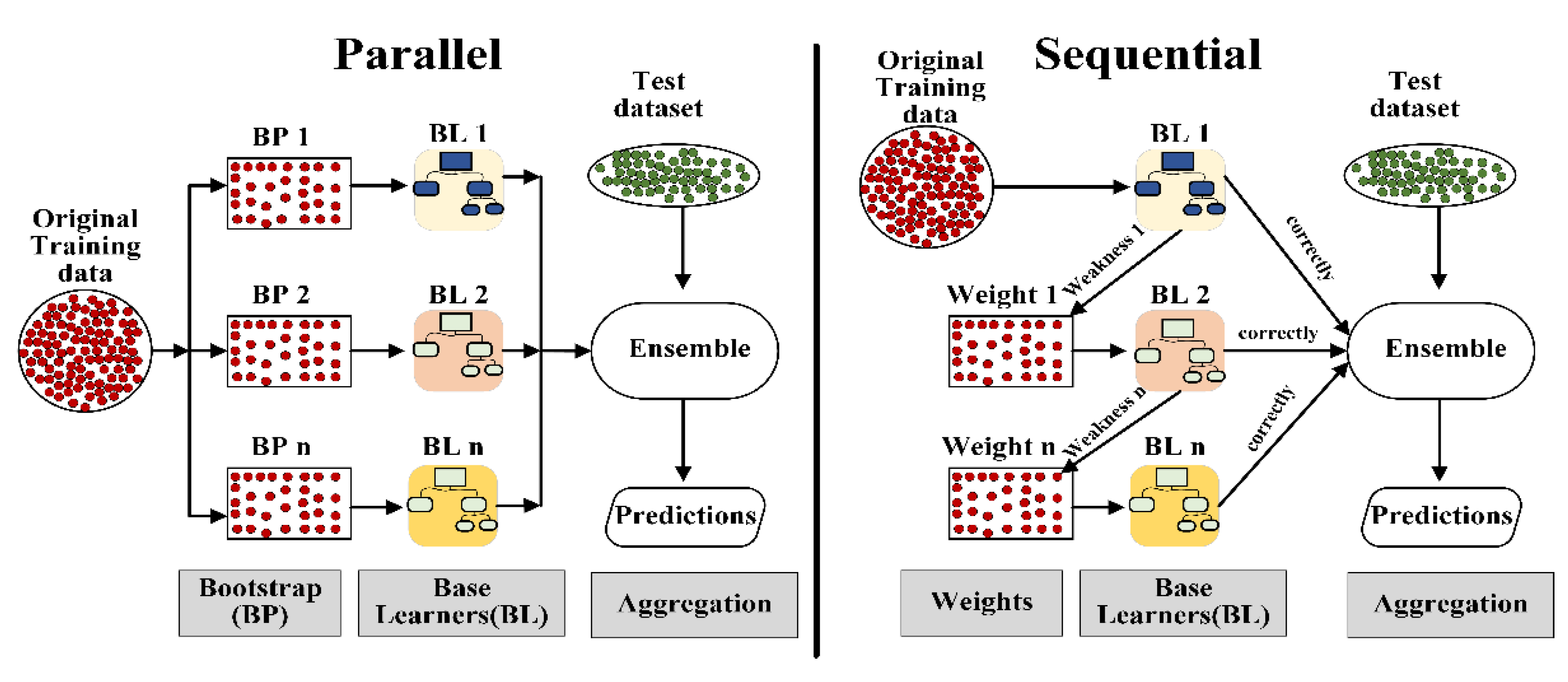
Figure 2.
Sketch of the proposed flow process to predict solar radiation applied ensemble learning algorithms.
Figure 2.
Sketch of the proposed flow process to predict solar radiation applied ensemble learning algorithms.
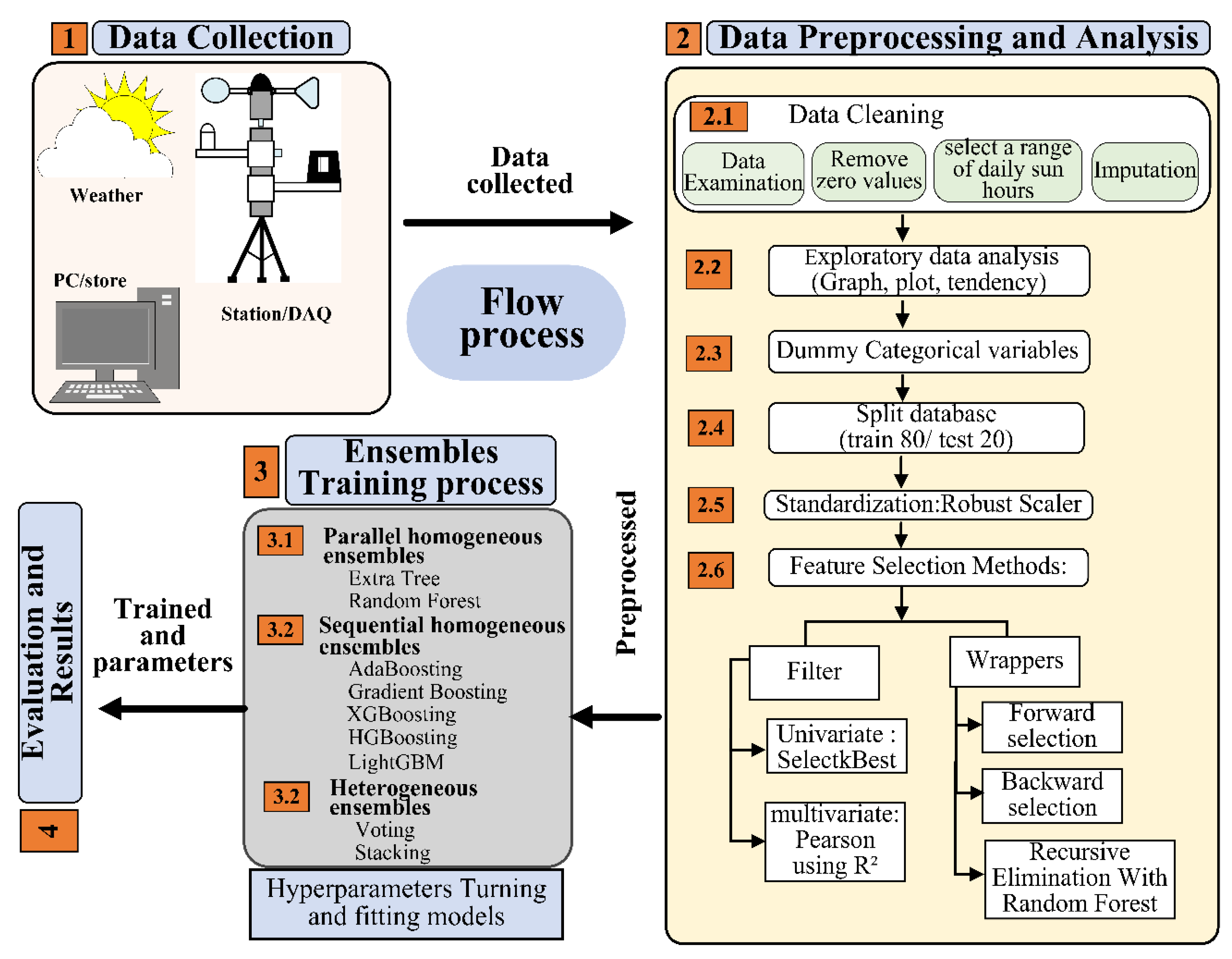
Figure 3.
GHI of Dominican Republic. map provided by the World Bank Group – Solargis [42].
Figure 3.
GHI of Dominican Republic. map provided by the World Bank Group – Solargis [42].
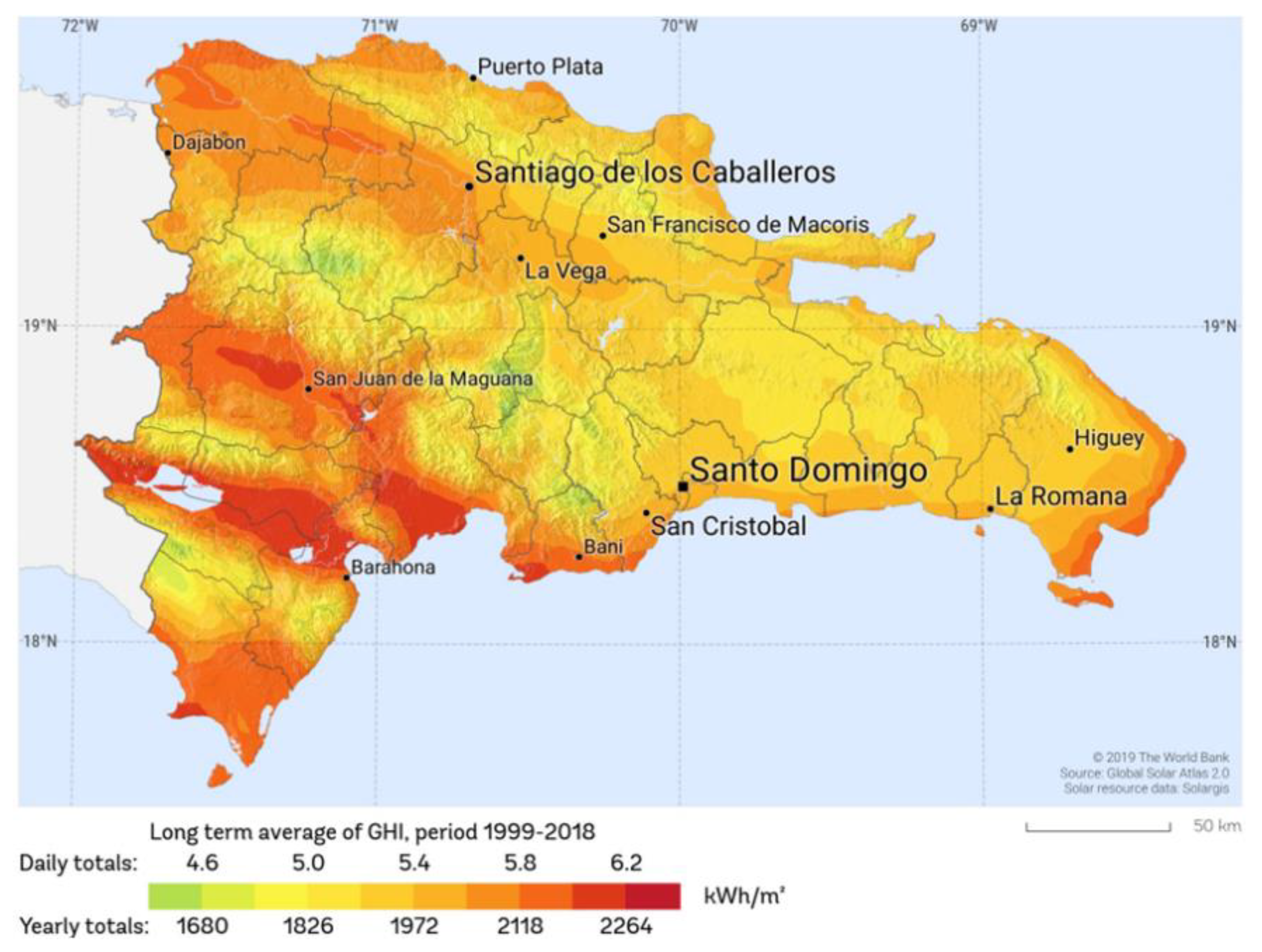
Figure 4.
Weather station mounted on the Roof FCSI building.
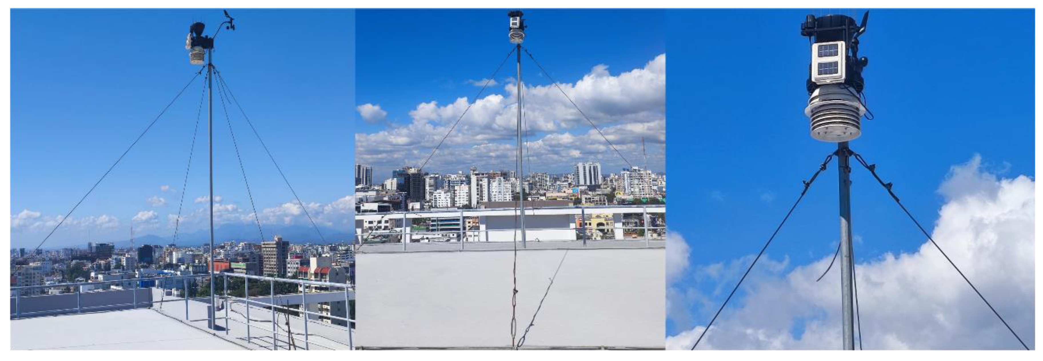
Figure 5.
Solar radiation: (a) grouped by wind direction (WD); (b) amount of observation by Wind Direction (WD).
Figure 5.
Solar radiation: (a) grouped by wind direction (WD); (b) amount of observation by Wind Direction (WD).
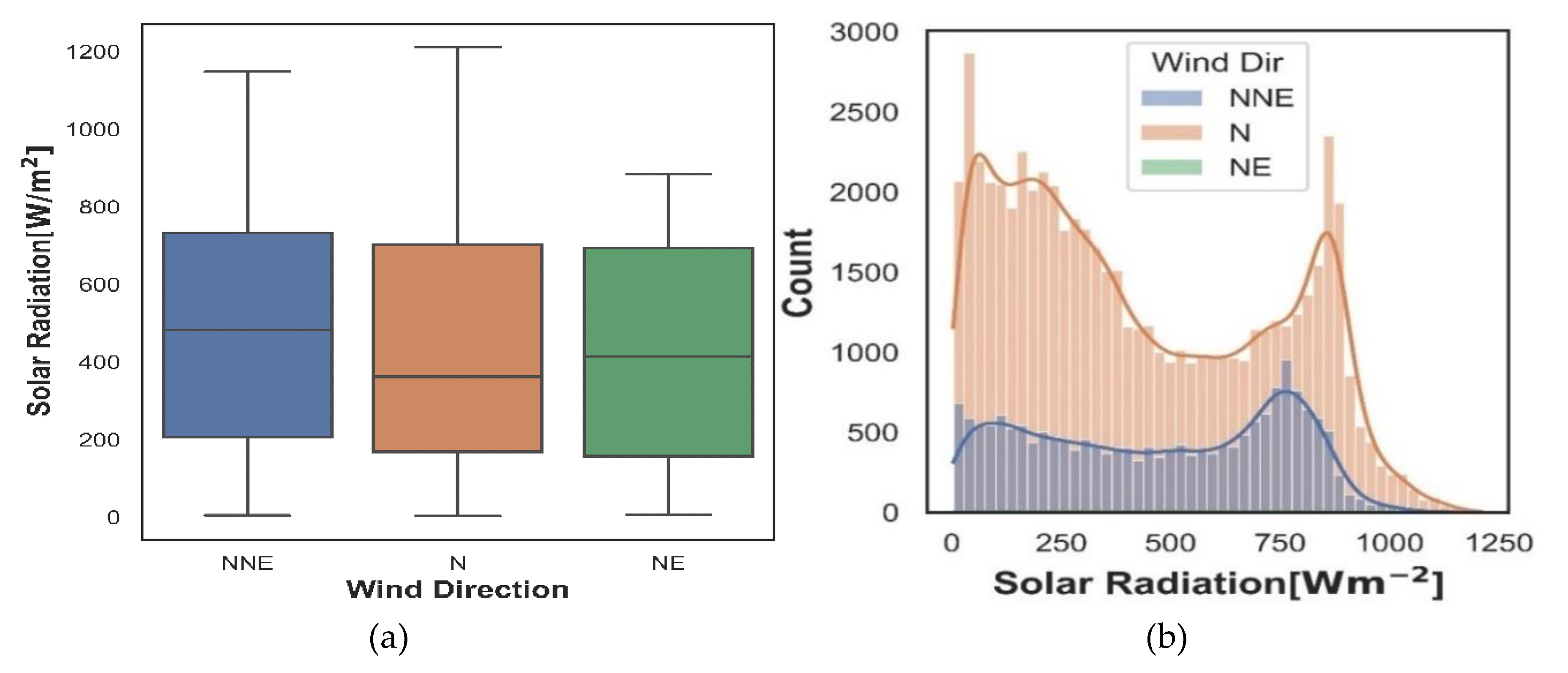
Figure 6.
Distribution of the solar radiation: (a) observations by wind direction for daily sun hours;(b) Average values for daily sun hours.
Figure 6.
Distribution of the solar radiation: (a) observations by wind direction for daily sun hours;(b) Average values for daily sun hours.
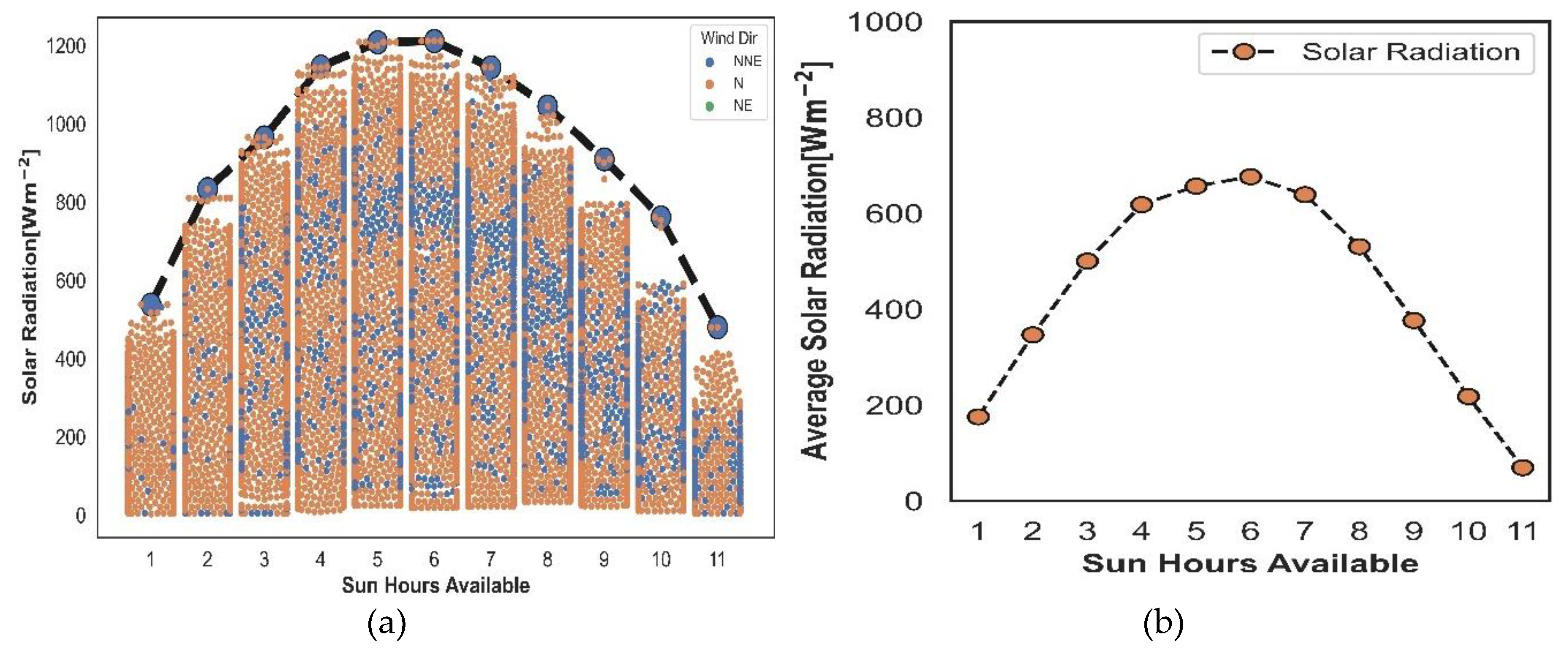
Figure 7.
Correlation matrix coefficient for all database using Pearson.
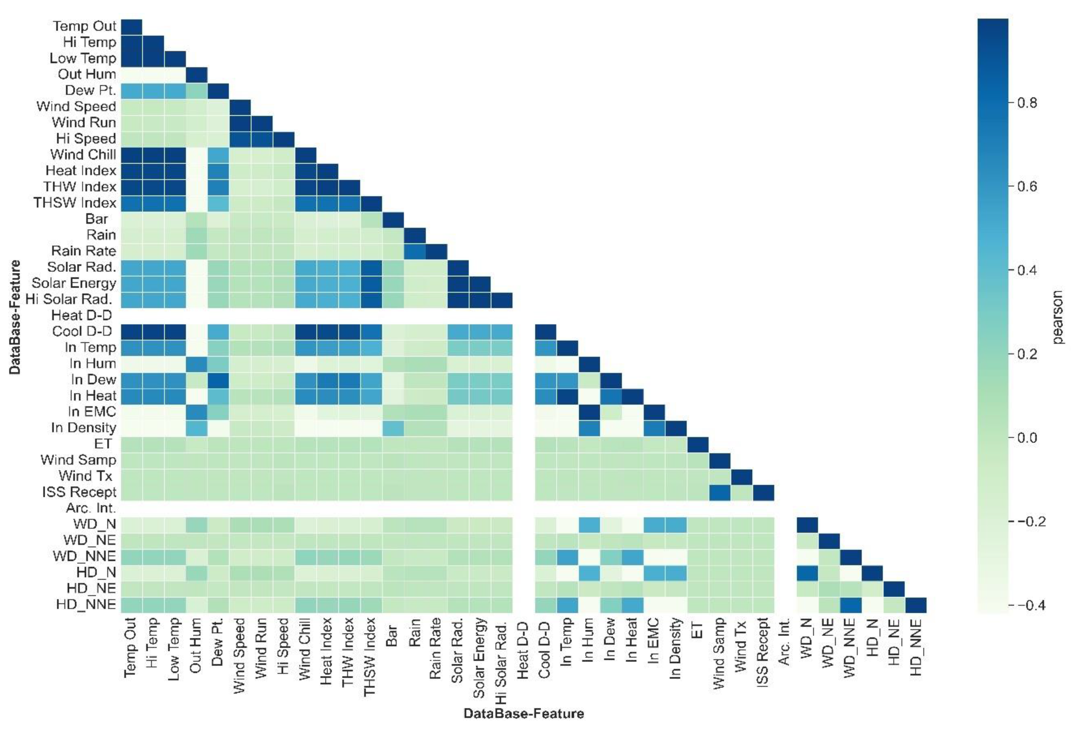
Figure 8.
Correlation matrix coefficient using Pearson after removing input parameters.
Figure 9.
Results of feature subset selection: (a) Selected by Pearson coefficient; (b) Relevance of features generated by RFE, only the most relevant were selected.
Figure 9.
Results of feature subset selection: (a) Selected by Pearson coefficient; (b) Relevance of features generated by RFE, only the most relevant were selected.
Figure 10.
Standardized distribution curve of the subset features selected.
Figure 11.
Comparison between measured and predicted solar radiation values with seven homogeneous ensemble learning; (a) RF; (b) ET; (c) XGB; (d) GB; (e) AGB; (f) HGB; (g) LGBM.
Figure 11.
Comparison between measured and predicted solar radiation values with seven homogeneous ensemble learning; (a) RF; (b) ET; (c) XGB; (d) GB; (e) AGB; (f) HGB; (g) LGBM.
Figure 12.
Evaluation of the measured vs predicted solar radiation values with two heterogeneous ensembles; (a) Stacking; (b) Voting.
Figure 12.
Evaluation of the measured vs predicted solar radiation values with two heterogeneous ensembles; (a) Stacking; (b) Voting.
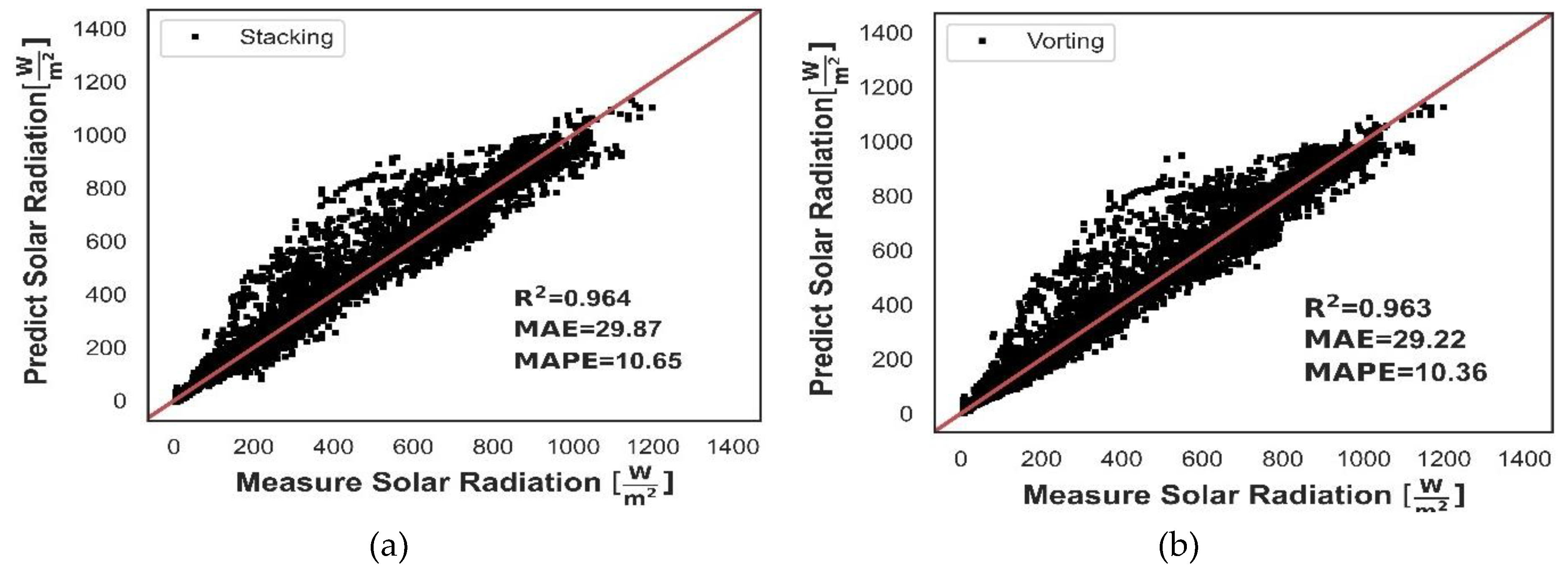
Figure 13.
Ability of the heterogenous Stacking ensemble to capture the tendency of solar radiation in several scenarios; (a) a day with good solar radiation (Date: May 5, 2022); (b) a day of scarcity solar radiation (May 8,2022); (c) a week with mixed behavior of the solar radiation (May 7-14, 2022).
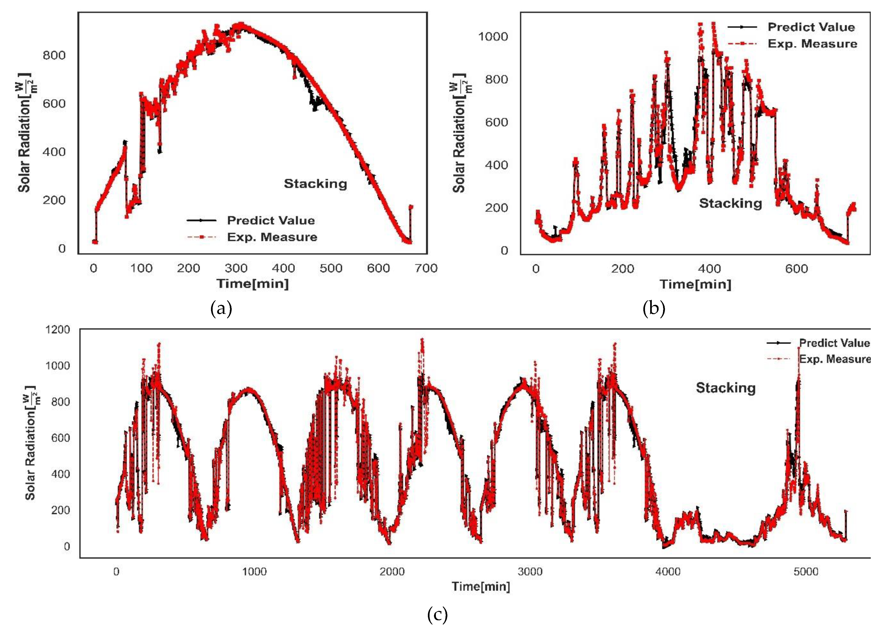

Table 1.
A review focused on recent studies using ensemble learning to predict solar radiation.
| Refs. | Location | Feature Subset selected |
Ensemble Algorithm test |
Time horizon | Data |
Periods | Metric |
Complete Preprocessing stage |
|---|---|---|---|---|---|---|---|---|
| 15 | Cairo, Ma’an, Ghardaia’ Tataouine, Tan-Tan |
4 | BG, GB, RF, SVM*, MLP-NN | 1 Hour | 71499 | 2010 to 2013 | MBE, R2 RMSE |
 |
| 3 | BG, GB, RF, SVM*, MLP-NN | 1 day | 7906 | |||||
| 16 | Odeillo (France) |
SP, MLP-NN, RF* | 1 to 6 hours | 10559 | 3 years | MAE, RMSE, nRMSE, nMAE | |
|
| 17 | Jeju Island (South Korea) |
330 | LGBM, RF, GB, DNN | 1 hour | 32,134 | 2011 to 2018 | MBE, RMSE, MAE, NRMSE |
|
| 18 | California, Texas, Washington, Florida, Pennsylvania, Minnesota |
9 | BS, BG, RF, GRF*, SVM, GPR | 1 hour | - | A year (TMY3) |
RMSE, MAPE, R2 | |
| 19 | New Delhi, Jaipur, Gangtok |
8 | Stacking*(XGB+DNN) | 1 hour | - | 2005 to 2014 | RMSE, MBE, R2 | ✓ |
| 20 | Bangladesh | 7 | GB*, AGB, RF, BG, | - | 3060 | 1999 to 2017 | MAPE, RMSE, MAE, R2 | |
| 21 | Ganzhou | 10 | GB*, XGB*, AB, RF, SVM, ELM, DT, KNN, MLR, RBFNN, BPNN | 1day | 13,100 | 1980 to 2016 | RMSE, MAE, R2 | |
| 1months | 432 | |||||||
| 22 | El Salvador (Brazilian) |
9 |
Voting*, XGB, RF CatBoost, AdaBoost, |
1 to 12 hours | MAE, MAPE, RMSE, R2 | ✓ | ||
| This Work | Santo Domingo |
8 | RF, ET, GB, XGB, HGB*, LGBM, Voting, Stacking* |
1-min | 78,536 | 5 months (2022) |
MSE, MAE RMSE, R2, MAPE |
✓ |
*ML algorithm with the best prediction performance.
Table 2.
Computational resources used to perform the simulation.
| Model | Processors | Memory | Graphics Card | Hard Disk |
|---|---|---|---|---|
| Dell OptiPlex 7000 | 12th Intel Core i7-12700 | 32GB DDR4 | Intel Integrated Graphics | 1TB PCIe NVMe |
Table 3.
characteristics of the parameters measured by weather station.
| Parameters /Features |
Description | Specifications | ||
|---|---|---|---|---|
| Range | accuracy (+/-) |
|||
| 1 | Date | month/day | 8 sec./ mon. |
|
| 2 | Time | 24 hours | 8sec./ mon. |
|
| 3 | Temp Out | Outside (Ambiental) Temperature | -40°C to 65°C | 0.3°C |
| 4 | Hi Temp | High Outside temperature recorded for a certain period | ||
| 5 | Low Temp | Low Outside temperature recorded for a certain period | ||
| 6 | In Temp | Inside Temperature/sensor located at the Console | 0°C to 60°C | 0.3°C |
| 7 | Out Hum | Outside Relative Humidity | 1% to 100% | 2% RH |
| 8 | In Hum | Inside Relative Humidity at the Console | 1% to 100% | 2% RH |
| 9 | Dew Pt. | Dew Point | -76°C to 54°C | 1°C |
| 10 | In Dew | Inside Dew Point at the Console | -76°C to 54°C | 1°C |
| 11 | Wind Speed | Speed of the outside local wind | 0 to 809 m/s | > 1 m/s |
| 12 | Hi Speed | High Velocity of the outside wind recorded in the configure period | ||
| 13 | Wind Dir | Wind direction | 0° to 360° | 3° |
| 14 | Hi Dir | High Wind direction recorded for a certain period | ||
| 15 | Wind Run | The “amount” of wind passing through the station/time | ||
| 16 | Wind Chill | Apparent temperature index calculated from wind speed and air temperature | -79°C to 57°C | 1°C; |
| 17 | Heat Index | An apparent temperature index estimated by associated temperature and relative humidity to determine the level of perceived air hot (feels) | -40°C to 74°C | 1°C |
| 18 | THW Index | use the temperature -humidity -wind to estimate apparent index | -68°C to 74°C | 2°C |
| 19 | THSW Index |
combine the temperature -humidity -sun-wind to estimate apparent temperature index (feels like out in the sun) | ||
| 20 | Bar | Barometric Pressure | 540 to 1100mb | 1.0 mb |
| 21 | Rain | The amount of rainfall Daily/monthly/yearly | to 6553 mm | > 4% |
| 22 | Rain Rate | Rainfall intensity | to 2438 mm/h | >5% |
| 23 | Solar Rad. | Solar Radiation, includes both the direct and diffuse components | 0 to 1800W/m2 | 5% FS |
| 24 | Hi Solar Rad. | High Solar Radiation recorded for a certain period | ||
| 25 | Solar Energy | The rate of solar radiation accumulated over a time | ||
| 26 | Heat D-D | Heating degree day | ||
| 27 | Cool D-D | Cooling degree days | ||
| 28 | In Heat | Inside heat index, where the console is located | -40°C to 74°C | |
| 29 | In EMC | Inside Electromagnetic Compatibility | ||
| 30 | In Density | Inside air density at the console installation location | 1 to 1.4 kg/m3 | 2% FS |
| 31 | ET | A measurement of the amount of water vapor returned to the air in a specific area through both evaporation and transpiration | to 1999.9 mm |
>5% |
| 32 | Wind Samp | wind speed samples in “Arc Int” amount of time | ||
| 33 | Wind Tx | RF channel for wind data | ||
| 34 | ISS Recept | % - RF reception | ||
| 35 | Arc. Int. | archival interval in minutes | ||
Table 4.
Evaluation results of the five subset feature selection methods.
| Selection Methods |
Subset of feature selected |
Characteristics | Ensemble learning Algorithms | Score R2 (test set) |
|---|---|---|---|---|
| Pearson | Temp Out, Out Hum, Dew Pt.,THSW Index, Bar, Rain, In Temp, In Density |
<-0.1 |
GB | 0.924 |
| AGB | 0.822 | |||
| XGB | 0.958 | |||
| ET | 0.958 | |||
| RF | 0.954 | |||
| RFE |
In Temp, In Density, Out Hum, Bar, THSW Index,Wind Speed,Dew Pt.,Temp Out |
External ML algorithm= RF, RF={ n_estimators:350, criterion:squared_error, max_depth:15, max_features:sqrt } |
GB | 0.930 |
| AGB | 0.843 | |||
| XGB | 0.962 | |||
| ET | 0.964 | |||
| RF | 0.960 | |||
| SKBest |
Temp Out, Out Hum, Dew Pt., Wind Speed, THSW Index, Bar, Rain, In Temp |
Score function=Regression, Number feature to select =8 |
GB | 0.929 |
| AGB | 0.843 | |||
| XGB | 0.962 | |||
| ET | 0.964 | |||
| RF | 0.959 | |||
| SFS-FW |
Temp Out, Out Hum, Dew Pt., Wind Speed, THSW Index, In Density, WD_NNE, HD_N | External ML Algorithm=LR, direction=forward, scoring=R2, cross validation=kfold, Kfold={ folds=5, shuffle=NO} |
GB | 0.930 |
| AGB | 0.833 | |||
| XGB | 0.962 | |||
| ET | 0.961 | |||
| RF | 0.957 | |||
| SFS-BW |
Temp Out, Out Hum, Dew Pt., Wind Speed, THSW Index, Bar, In Temp, In Density |
External ML Algorithm=LR, direction=backward, scoring=R2, cross, validation=Kfold, Kfold={folds=5, shuffle=NO} |
GB | 0.930 |
| AGB | 0.833 | |||
| XGB | 0.962 | |||
| ET | 0.962 | |||
| RF | 0.957 |
Table 5.
Specification of the hyperparameter turning process for ensemble learning algorithms.
| Algorithms | Iteration (n_iter)/ Cores |
Appropriate Hyperparameters | Computational cost(s) |
|---|---|---|---|
| RF | 1000/8 | n_estimators: 1160, max_features: 8, min_samples_leaf: 7, max_depth: 17 , min_samples_split: 10 |
51605.280 |
| ET | 1000/8 | n_estimators: 630, min_samples_split: 10, min_samples_leaf: 1, max_depth: 23 max_features: 8 |
126830.010 |
| AGB | 250/8 | n_estimators: 100, loss: exponential, learning_rate: 0.201 | 10877.330 |
| GB | 1500/8 | n_estimators: 2200, min_weight_fraction_leaf: 0, min_samples_split: 250, min_samples_leaf: 40, max_leaf_nodes: 10, max_features: 8, max_depth: 18, loss: huber, learning_rate: 0.101, criterion: friedman_mse, alpha: 0.210, tol: 1e-06, subsample: 0.1, |
16221.750 |
| XGB | 1500/8 | tree_method=hist, n_estimators: 2600, subsample: 0.9, scale_pos_weight: 0.05, reg_lambda: 0.89, reg_alpha: 0.2, min_child_weight: 10, max_depth: 5, learning_rate’: 0.01, gamma’: 0.05, colsample_bytree’: 0.79 |
56941.400 |
| HGB | 1500/8 | quantile: 1, min_samples_leaf: 49, max_iter: 680, max_depth: 5, loss: absolute_error, learning_rate: 0.101, l2_regularization: 0.0 | 10296.756 |
| LIGHTBM | 1500/8 | n_estimators: 2200, boosting_type :dart, subsample_freq: 4, subsample’: 0.5, reg_lambda: 2.40 ,reg_alpha’: 0.0, num_leaves: 31, min_sum_hessian_in_leaf’: 19, min_data_in_leaf’: 21, max_depth: 10, max_bin: 70, learning_rate: 0.1, colsample_bytree: 0.5, bagging_seed: 96, bagging_freq: 6, bagging_fraction’: 0.3, objective:‘regression’, force_row_wise:True, | 126833.010 |
| Voting | /8 | Average output results:{ HGB,ET,GB,RF} | 900.541 |
| Stacking | /8 | Combining algorithm-Layer 1:{ HGB,ET,GB,RF}, Layer-2:{LinearRegressor} Cross-validation: KFold{five folds without shuffle} |
2100.780 |
Table 6.
Evaluation metrics for each ensemble learning built.
|
Ensemble Learning |
Test set | ||||
|---|---|---|---|---|---|
| Evaluation metrics | |||||
| MSE [W2/m4] |
RMSE [W/m2] |
MAE [W/m2] |
MAPE [%] |
R2 [-] |
|
| RF | 4243.296 | 65.141 | 33.745 | 9.20 | 0.9538 |
| ET | 3795.275 | 61.606 | 30.722 | 8.40 | 0.9584 |
| XGB | 3515.760 | 59.294 | 33.460 | 12.90 | 0.9608 |
| AGB | 8739.339 | 93.484 | 70.992 | 49.11 | 0.9027 |
| GB | 3499.137 | 59.154 | 31.977 | 11.8 | 0.9610 |
| HGB | 3308.874 | 57.523 | 30.839 | 10.7 | 0.9631 |
| LGBM | 3494.692 | 59.116 | 33.883 | 16.00 | 0.9611 |
| Stacking | 3218.265 | 56.730 | 29.872 | 10.60 | 0.9645 |
| Voting | 3346.470 | 57.849 | 29.220 | 10.40 | 0.9627 |
Disclaimer/Publisher’s Note: The statements, opinions and data contained in all publications are solely those of the individual author(s) and contributor(s) and not of MDPI and/or the editor(s). MDPI and/or the editor(s) disclaim responsibility for any injury to people or property resulting from any ideas, methods, instructions or products referred to in the content. |
© 2024 by the authors. Licensee MDPI, Basel, Switzerland. This article is an open access article distributed under the terms and conditions of the Creative Commons Attribution (CC BY) license (http://creativecommons.org/licenses/by/4.0/).
Copyright: This open access article is published under a Creative Commons CC BY 4.0 license, which permit the free download, distribution, and reuse, provided that the author and preprint are cited in any reuse.


