
Submitted:
12 July 2024
Posted:
17 July 2024
You are already at the latest version
Abstract
Asphaltene-resin-paraffin deposition (ARPD) is a complicated and prevalent issue in oil and gas industry, impacting the efficiency, integrity of petroleum extraction, production, transportation and processing systems. Considering all witnessed ARPD problems in Azerbaijan oil fields, this paper proposed a chemical method and optimized the type and the concentration of chemical inhibitors. And then the effect of selected chemical reagent on inhibiting the ARPD amount and thus en-hancing oil recovery was detected by reservoir simulation during both waterflooding and CO2 flooding production. Three new chemical compounds (namely, Chemical-A, Chemical-B and Chemical-C) were examined in laboratory conditions and their impact on rheological properties of high-paraffin oilfield samples of Azerbaijan (X, Y and Z) were investigated. Experimental results show that Chemical-C with concentration of 600 g/t has the best efficiency for alleviating the problems. After adding Chemical-C to the crude oil, the freezing point of oil is decreased from 12 °C to (-4) °C, ARPD amount is declined from 0.185 to 0.016 g and oil effective viscosity is reduced from 16.2 mPa·s to 3.1 mPa·s. It is determined that for water and CO2 flooding, higher injection pressure resulted in reduced asphaltene precipitation. Adding selected ARPD inhibitor, the oil recovery for waterflooding can increase from 52% to 62%, while it can rise from 55% to 68% for CO2 flooding.
Keywords:
asphaltene-resin-paraffin deposition (ARPD)
; rheological properties
; freezing point
; enhanced oil recovery
1. Introduction
Asphaltene, resin, and paraffin deposits present significant challenges in the petroleum industry, causing blockages and reducing the efficiency of oil production and transportation. In bottomhole section of well, on the surfaces of well equipment, on the walls of tubing string, in places where oil has settled, asphaltene-resin-paraffin deposits (ARPD) can often be found. Almost all oil fields face this kind of severe problems. It is reported that this problem is encountered very often in Baku (Azerbaijan) and Grozny (Russia) oilfields. The main problems in Baku oil fields were caused by salt and in separate oil fields with paraffin deposits. In the Grozny oil fields, due to the high temperature, paraffin precipitation was not observed in the wells, nevertheless, the well flowlines were often subjected to paraffinization [1,2,3].
At present, there are various theories that explain the formation of ARPD based on modern concepts. Among them, a relatively widespread theory explains the formation process of oil deposits from the view of crystallization temperature of solid paraffin-naphthenic hydrocarbons. This theory, however, does not account for critical factors such as adhesion, adsorption, and the influence of resin-asphaltene components on oil-dispersed systems [4,5,6,7]. In contrast, another advanced theory highlights the significant influence of ARPD on the paraffinization process of oil field equipment. The authors of this theory explain the formation of paraffin deposits through the effects of coagulation, aggregation, micelle-forming properties of naphthenic hydrocarbons and asphaltenes in oil-dispersed systems [8]. Additionally, this theory considers the dynamic interactions between these components and the equipment surfaces, emphasizing the complexity of the deposition process. The theory suggests that understanding these interactions is essential for developing more effective strategies to mitigate ARPD formation and improve the efficiency of oil production operations. By incorporating these factors, it can be better predicted and controlled the conditions under which ARPD forms, leading to more targeted and effective prevention methods [9,10,11].
Currently, the prevailing approach for removing ARPD is considered the application of chemical methods, particularly chemical inhibitors. ARPD inhibitors are used to effectively dissolve and disperse asphaltene, resin and paraffin deposits that can accumulate in production wells and pipelines. By inhibiting the agglomeration of these compounds, ARPD inhibitors prevent the formation of blockages and flow restrictions, ensuring sustainable production and transportation of crude oil. This technology helps maintain operational efficiency, reduces downtime for maintenance, and minimizes the need for costly interventions such as mechanical cleaning or chemical treatments [12].
To address the challenge of asphaltene, resin, paraffin deposits in the petroleum industry, this study integrates laboratory experiments and numerical simulations to optimize a chemical method. By integrating laboratory experiments with reservoir simulations, the research offers a practical and reliable methodology for selecting the most effective reagent and predicting its performance in real reservoir conditions. The findings of this study not only contribute to improving the efficiency of ARPD removal processes but also enhance overall petroleum production operations, leading to cost savings, increased productivity and prolonged reservoir condition.
2. Materials and Methods
2.1. Materials
In this study, new oil-based ARPD inhibitors were proposed and developed using depressor additive of Difron-3970 and reagents of BAF-1, D1, and Gossypol, respectively. They were labeled as Chemical-A, Chemical-B, and Chemical-C, respectively. The efficient ratios of chosen chemical inhibitors studied and it is determined that for Chemical-A the best ratio is BAF-1 + Difron-3970 = 1:1, for Chemical-B is D1 + Difron-3970 = 3:1, for Chemical-C is Gossypol + Difron-3970 = 4:1. Therefore, the effects of these inhibitors at specified ratios were thoroughly studied for this investigation.
Oil sample analyzed in this paper was collected from Azerbaijan oilfield, referenced as X. The crude oil used in this study was sampled from downhole conditions to ensure it was representative of the actual reservoir fluid. By sampling directly from downhole minimized the risk of prior asphaltene or paraffin deposition, which can occur during surface handling and transportation. The reservoir temperature is 55 °C, reservoir pressure is 16.8 MPa. The physicochemical properties of the high-paraffin oilfield sample are listed following Table 1:
As can be seen from the table, the content of asphaltene, paraffin and resin components for taken oilfield sample are quite high. It is characterized with high freezing point. Therefore, asphaltene-resin-paraffin deposits are formed as soon as the temperature drops below the freezing point during production, storage and transportation of these oil samples.
2.2. Methodology
2.2.1. Oil Example`s Freezing Point Determination
Within study, a temperature range of 0-60 °C was chosen for all experiments to align closely with the actual reservoir conditions of taken oilfield samples. Throughout the analysis, oil reservoirs have a temperature of overall 50 °C. By water injection, this temperature could be lowered, promoting asphaltene deposition. As oil is produced and transported through the wellbore, the temperature changes further, increasing the possibility of asphaltene precipitation due to reduced solubility at lower temperatures.
In laboratory conditions, the freezing point of oil examples without and with reagents was performed according to RD 39-3-812-82 methodology [12]. A 100 ml of oil sample was poured into spherical test tubes with a diameter of 20 mm and a height of 160 mm, heated to a temperature of 55-60 °C. Chemical compounds of various concentrations were added to it and gradually cooled to a temperature of 30-40 °C (for conducting comparison, one test tube was not added chemical compound). Then the test tubes were placed in the thermostat and the cooling process was continued. As the temperature gradually dropped, precise measurements were taken at intervals of every three degrees Celsius. At each interval, the test tubes were tilted to a 90° angle to ensure uniform distribution of the oil within the tube. In such successive inspections, the temperature at which the level of oil in the test bottles is stationary was noted and at this time, the test bottle was kept in a horizontal position for 5 seconds, and the complete solidification of the liquid was determined due to the immobility of the upper liquid layer [13] (Figure 1).
2.2.2. Determination of Oil Deposits Quantity
The aim of the “cold finger test” method is to determine the quantity of asphaltene-resin-paraffin substances deposited from oil on a cooled metal surface. In the "cold finger test" method, all stages such as the formation and accumulation of ARPD, including processes such as sediments dispersion due to oil flow effect, the precipitation, growth of heavy components of oil, paraffin crystals and the crystallization centers formation are realized.
Studied oil sample with volume of 100 ml is poured into chemical metal cups with the same proportion (d=36 mm, ℓ=130 mm) equipped with a magnetic stirrer intended for the experiment (Figure 2). Then the oil in the chemical cups is heated to 50-55 °C with stirring at 350 rpm using a magnetic stirrer to ensure a good reagent distribution throughout the oil volume and a pre-calculated amount of the chemical compound is added to each sample (chemical compound is not added to one of the cups intentionally for comparison purpose). The chemical cups are placed in an external thermostat, and a stainless-steel U-shaped tube (d=15 mm, ℓ=110 mm) was inserted into it. The "cold finger" surface provides a temperature gradient with the liquid, which is perfect for the precipitation and crystallization of high-molecular oil components. The asphaltene-resin-paraffin precipitations are liquefied by heating the "cold finger" to 70 °C using a cryostat, and the precipitation mass is measured using the gravimetric technique [14]. The experiment duration is 40 minutes.
2.2.3. Determination Method of Effective Viscosity, Limiting Shear Stress and Non- Newtonian Index
The method is conducted by using rotational viscometer, brand of the “Rheotest 2.1” or its subsequent modifications with measuring devices - a special cylindrical and a cone-plate (Figure 3).
Prior to experimentation, the preparation of the sample fluid is conducted maintaining its temperature and purity. The viscometer is calibrated meticulously according to manufacturer guidelines and precise temperature control mechanisms are employed. Initial torque and rotational speed readings are recorded before gradually increasing rotational speed, recording torque at each increment to cover a range of shear rates. Rigorous data analysis techniques are proceeded to calculate shear rate and subsequently determine effective viscosity. In laboratory conditions, the research process is carried out in a wide temperature range (0, 10, 20, 30, 40 and 50 °С) in "Rheotest-2.1" viscometer with 100 ml of oil samples. The experiment duration is 2 hours. According to device results, non-Newtonian index is taken and processing. Within the framework of the Gersel-Balkley model, the value of the effective viscosity depending on the temperature is calculated by the following expression [15]:
μe - effective viscosity, Pa·s, τ - shear stress, Pa, τ0 - limit shear stress, Pa, γ - velocity gradient, s-1, K - consistency, (Pa·s), (the higher liquid viscosity means the greater K value), n - non-Newtonian index, (the more n is different from 1, the more non-Newtonian properties increase).
2.2.4. Corrosion Rate Determination by Gravimetric Method
Assessing reagent's effectiveness for inhibiting corrosion is crucial for understanding its potential to reduce metal corrosion rates in various aggressive environments, helping optimize the reagents for industrial applications, where material durability and reliability are key factors. The essence of the gravimetric test method is based on determining the mass loss of metal samples during their stay in the tested corrosion environment. In laboratory conditions, gravimetric tests are carried out in accordance with the requirements of relevant methodology [16,17].
During the experiment, samples are used which prepared in the form of plates from different steel brands with 100 ml volume of reagents. The duration of experiment is 10-12 hours. The average static relative error of measuring steel samples corrosion rate is not higher than 0.5%. Ct20 steel samples, with dimensions of 30×20×1 mm were used during the research. Table 2 shows the chemical composition of Ct20 brand steel.
To determine the corrosion rate by the gravimetric method, firstly steel samples are prepared by cutting, shaping and cleaning them with sandpaper and acetone, then dry and accurately weigh each sample to record the initial mass (m0). Submerge the specimens in a prepared corrosive solution for a specified duration, ensuring they are fully immersed and maintained under consistent environmental conditions. After the exposure period, remove the samples, rinse with distilled water, clean to remove corrosion products without affecting the base metal, dry thoroughly and reweigh to obtain the final mass (m1). The area of the samples taken for testing is calculated according to the following formula:
Sn - area of steel sample, mm2, a - the length of sample, mm, b - width of sample, mm, h - height of sample, mm.
Since a=30 mm, b=20 mm, h=1 mm, steel sample area taken for testing is determined as SN=2·30·1+2·30·20+2·20·1=1300 mm2=0.0013 m2.
Metal loss is calculated for three steel plates and the average mass is found. During gravimetric tests, the corrosion rate mass indicator in both without reagent and with reagent condition is characterized by Km and is calculated by the following mathematical equation:
Km - corrosion rate mass index, g/m2·hr, m0 - the mass of the sample before the tests, g; m1 - mass of the sample after the tests, S - average surface area calculated for three samples, m2; τ - duration of the test, hrs.
The protection effect of reagent is calculated as:
Z - protection effect, %, K0 – corrosion rate without reagent, g/m2·hr, Kinh - corrosion rate with reagent, g/m2·hr.
3. Experimental Results
3.1. Effect of Compound Chemicals for Oil Examples Freezing Point
It is obviously seen from the Figure 4, as the concentrations of Chemicals A, B and C increase, its effect on oil freezing point increases first then decreases. In the range of compound chemicals concentration 200-1000 g/t, the freezing point varied between 12-0, 12-2, 12-(-1) °С, for the three types chemicals, respectively. Additionally, it should be noted that for Chemical – A after the 800 g/t, for Chemical – B 500 g/t, for Chemical – C 600 g/t, the freezing point of mentioned oil examples increases, as a result, it is determined that the best effect occurs for mentioned concentration rates, which means that they are optimal concentration amounts for these compound chemicals. Among three chemical compounds Chemical-C had great impact on freezing point of oil sample, which reduced it by 13 °С. The other experiments were then carried out on samples with its determined optimal concentration rates, which were respectively 800, 500 and 600 g/t of Chemicals A, B and C.
3.2. Effect of Compound Chemicals for Oil Examples Deposition
The effect of compound chemicals on asphaltene, paraffin, resin deposits (ARPD) in the oil samples was studied by the "cold finger test" method. Experiments were carried out in the temperature range of 5-50 °C on oil sample without and with compound chemical (Figure 5). It can be noticed that from the graph, in case of without use of any compound chemical, the amount of ARPD decreases as temperature increases and ARPD amount over temperature changes between 0.338 – 0.031 g.
After application of 800 g/t concentration Chemical-A, the ARPD amount at 5 °С becomes 0.209 g and at the final situation, for 50 °С, the value decreases to 0.018 g. When it comes to Chemical-B with 500 g/t and Chemical-C with 600 g/t the depositions decline from 0.243 g to 0.022 g and from 0.185 g to 0.016 g, respectively. Chemical-C efficiency is better than the other two chemicals, which reduced ARPD amount almost 48% for final condition.
3.3. Effect of Compound Chemicals for Oil Example`s EFFECTIVE viscosity
Figure 6 illustrates that before application of chemicals, the effective viscosity for the oil is varied from 29.2 to 5.9 mPa·s as temperature changes from 5 °C of 60 °C.
After application of each chemical compound with its optimal concentration rates, the oil viscosity reduction is obviously observed. Chemical-C declined the effective viscosity of oil from 16.2 to 3.1 mPa·s, which performs the best than the other two chemicals.
3.4. Effect of Compound Chemicals for Oil Examples Corrosion
Determination of corrosion rate is conducted by gravimetric method according to methodology and results are provided in Figure 7. It is observed that the simultaneously protective effect increases with the Chemical-A concentration rises in the range of 200-1000 g/t. The highest protective effect, about 95.4% was obtained at a concentration of 800 g/t of chemical compound. After 800 g /t concentration rate of compound chemical, the effect of it getting reduce for corrosion rate. For Chemical-B and Chemical-C the highest protective rates from corrosion are obtained 91.8 and 98.1% with their optimal concentration rates, which are 500 and 600 g/t, respectively. So Chemical-C has the best protective effect among the three chemicals.
3.5. Effect of Compound Chemicals for Limiting Shear Stress and Non-Newtonian Index
The experiments were conducted at the oil temperatures of 5,10, 20, 30, 40 and 50 °C. Experiments were carried out on samples with its determined optimal concentration rates, which were respectively 800, 500 and 600 g/t of Chemicals A, B and C added form. For all chemical compounds, when the oil temperature is 40 and 50 °C, experimental values of limit shear stress are very close to 0 and experimental values of non-Newtonian index are almost 1, which are signs of Newtonian liquid which easily flows. Below 40 °C, it is obvious that non-Newtonian index becomes notable which is sign of flowing liquid. Consequently, according to the results of non-Newtonian index and limiting shear stress, it is apparent that oil becomes flow from low temperatures, which means viscosity decrease (Table 3). If the correlate the results, it presents information that compare with other chemical compounds, while application of Chemical-C, oil becomes to flow at a temperature much lower than the freezing temperature of high-paraffin oil and at that situation liquid properties are moderately better for easy flow.
3.6. Effect of Compound Chemicals for Y and Z Oilfield Samples` Rheological properties
For next, to analysis taken chemical compositions affect for other 2 high-paraffin oilfields samples of Azerbaijan (Y and Z oilfields), the laboratory experiments were conducted according to previously mentioned methodology. The taken high-paraffin oilfield samples` physicochemical properties are described as follow:
Table 4 demonstrates that taken other 2 oilfield samples also are high-paraffin oils with their notably physicochemical properties. The reservoir temperatures for Y and Z are 48 and 44 °C, reservoir pressures are 16.1 and 15.3 MPa, respectively. As following the same procedure for primary oilfield sample, mentioned samples were also taken directly from downhole conditions. Their freezing point are quite high, which is very convenient condition for ARP deposition.
Table 5 depicts that studied chemicals also very efficient for these oil samples, which reduced the freezing point considerably and avoid paraffin deposition noticeably. ARPD amount for Y and Z oilfields reduced by overall 35% and 37%, respectively after application of the chemicals, and again Chemical-C performs the best. Additionally, it's essential to emphasize that starting from 30-40 °C, taken oil samples displayed Newtonian characteristics, maintaining a constant viscosity across varying shear rates with Chemical-A and Chemical-B application. However, after application of Chemical-C, it is witnessed that, transition temperature is already 20 °C, which is quite successful result to achieve Newtonian liquid characteristics for lower temperature conditions.
4. Investigation of Enhanced Oil Recovery Effect by Injecting Paraffin Inhibitors during Waterflooding and CO2 Flooding Based on Numerical Simulation
Modern petroleum industry developments have several opportunities, such as creating simulation models to anticipate asphaltene precipitation. However, in this situation there is a challenge as asphaltenic fluids are complex and in turn it needs complex models to be represented. The modeling of asphaltenic fluids evolved comprehensive thermodynamics, beginning with simple solubility parameters, regular solutions and currently progressing to various modes of SAFT (Statistical Association of Fluid Theory). SAFT is a broadly used EOS for characterizing the behavior of the asphaltene phase that is based on statistical mechanics. The initial stage SAFT EOS is determination of a reference fluid that serves as a stand-in for the original fluid.
The GEM simulator in the commercial simulation software (CMG) is used in this simulation investigation. GEM and Winprop simulators are used to emulate asphaltene precipitation, which is considered during waterflooding and CO2 flooding. Asphaltene formation mechanism and its impact in the reservoir are studied. It should be mentioned that fluid modeling data is the essential and most crucial data for the research (as Table 6). “X1” oilfield sample from Azerbaijan was used and examined in our case study.
4.1. Asphaltene Precipitation Modeling in CMG
Winprop was used to simulate the asphaltene related issues for reservoir oil. Nghiem proposed the asphaltene precipitation model using WinProp simulator [18]. Previous models presumed that asphaltene was the heaviest component of oil. The heaviest component is divided into two parts: non-precipitating components (i.e., C31+) and precipitating components (i.e., asphaltene), which share the same critical properties and acentric factors, but they interact differently with the light components. The non-precipitating components are considered namely, resins and heavy paraffins. This phase is known as the asphaltene part and its fugacity is described as follow:
This fugacity equation is true for both liquid and solid state asphaltene. The asphaltene stage can be classified as liquid or solid phase. As can be seen from the equation (5), fs* is referred to as the reference (asphaltene) fugacity, P* and T reference pressure and temperature, which can be determined by experimental solubility data and Vs is the solid (asphaltene) molar volume. Asphaltene will precipitate, if solid component fugacity is less than other two phases.
4.1.1. Fluid Characterization
The pseudo-components of C7+ is divided into a fraction along C31+ (Figure 8). The two-stage exponent was used in order to define the molar distribution weight while the splitting process. After dividing the (C7+) fraction, the single carbon number were splitted to four pseudo-components, using Lee-Kesler (1975) approach for determination of their critical properties and mixing rule correlation, updated after running to reflect the divided measurement results [19].
4.1.2. Prediction of Asphaltene Precipitation Behavior
Prediction related to asphaltene precipitation were made by clarifying flash calculation results with different pressure ranges. For low pressure conditions, the precipitation content was inaccurate. Because, it failed to forecast the offset pressure. To achieve perfect precipitation curve, some parameters need to be adjusted. As a result of numerous tests with various solid molar and the interaction parameters, the derived curve was obtained (Figure 9). The precipitation of asphaltene model predicts a pressure of 4500 psia for the onset pressure and for the offset 1500 psia, highest precipitation occurring around 2960 psia, near saturation pressure.
In Azerbaijan oil industry experience, waterflooding is a preferred secondary oil recovery technique over others. This preference primarily originates from waterflooding being a cost-effective and readily available option, furthermore through extensive utilization and optimization over the years. Additionally, CO2 flooding can contribute to both enhanced oil recovery and greenhouse gas mitigation efforts, making it a promising approach for addressing environmental challenges. That is why, in numerical simulation part of paper, firstly waterflooding, then CO2 flooding was run and provided comparative outcomes.
4.2. Reservoir Modeling
A 3D model was created using Builder with dimensions of 250 ft x 250 ft x 6 ft and 3750 grid cells. The Z direction consists of 6 equal layers. The homogeneous reservoir has a permeability of 300 mD in the X and Y directions and 50 mD in the Z direction, with all grid blocks having a porosity of 0.25. In CMG's Builder tool, the reservoir simulator is configured as shown in Figure 10, which includes the reservoir and well properties. Builder computes the rock-fluid interactions, while WinProp models the fluid for CO2 flooding and waterflooding simulations using GEM. The producer well is located in grid block 25, 25, 1 with a constant bottom hole pressure of 2000 psia, and the injector well is in grid block 1, 1, 1. The simulations, visualized in the figure below, include waterflooding and CO2 flooding, both with and without asphaltene precipitation.
4.3. Simulation of Asphaltene Deposition during Waterflooding
The simulation was run with a rate of 2000 bbl/day and a pressure of 3000 psia, for 10 years with and without asphaltene precipitation. The results of the simulation are shown below:
Figure 11 shows that the recovery factor of water flooding considering asphaltene is almost 12% lower than that without asphaltene form.
The Figure 12 shows asphaltene precipitation during water flooding with initial very low deposition (a) and occasional drops near injection and producer at the end of 10-year production (b). Water in oil reservoirs can alter asphaltene stability affecting reservoir fluid characteristics. High asphaltene deposition occurs at block pressures of 2500 and 3000 psia causing liquid phase to cohabit and indicating a thermodynamic imbalance in the asphaltic oil system. The lower recovery factor observed during waterflooding with asphaltene precipitation can be explained with several mechanisms. Asphaltene particles precipitate within the reservoir, leading to permeability reduction by blocking pore spaces and impeding oil flow to production wells. This restriction in permeability limits oil movement, resulting in decreased recovery. Furthermore, asphaltene accumulation near production wells obstructs flow paths, causing productivity losses and reducing oil extraction efficiency. Other potential reasons could include formation damage caused by asphaltene deposition, altering the reservoir's fluid flow dynamics and changes in fluid properties, such as viscosity, which directly affect oil displacement and recovery.
4.4. Simulation of Asphaltene Deposition during CO2 Flooding
The GEM model of CMG software was used to simulate CO2 flooding, adjusting the EOS with the WinProp module. Model parameters like porosity and permeability were correlated, and reservoir pressure was used for miscible flooding processes. A 3D numerical model was set up and run for 10 years with constant gas injection, both with and without asphaltene. CO2 was injected at pressures of 2500 psia, 3000 psia, and 4000 psia, but while simulation 3000 psia pressure have been maintained, close to the bubble point pressure.
Using 3000 psia as injection pressure, the comparison of the recovery factor conducted for the CO2 flooding with and without considering asphaltene precipitation. The results demonstrate that for both injection processes, higher pressure leads to improved recovery factor. It shows that high pressure injection reduces asphaltene precipitation and thus enhance oil recovery (Figure 13 and Figure 14).
Figure 14 depicts asphaltene precipitation deposition while CO2 flooding. As we can see, (a) represents the start of the simulation, which is almost typical no asphaltene deposition. However, at the end of the simulation (b), there are some asphaltene drops in the reservoir near the injection and the producer due to temperature and pressure change.
4.5. Simulation of Asphaltene Deposition during Waterflooding and CO2 Flooding with Reagent
While addition of the chemical reagent to the numerical simulation, the approach which expresses that asphaltene in solution behaves as a fluid component, was followed and applied. Chemical reagent was treated as a composition of fluid component. It involved defining the chemical reagent's properties and interactions using the WinProp module and adjusting the EOS to reflect its impact on asphaltene solubility and stability. The reagent was then introduced into the simulation model as an additive to the injection fluid, either mixed with the injected water for waterflooding or combined with the CO2 while CO2 flooding. According to experimental results, the best effective reagent (Chemical-C) was chosen for application of reservoir simulation during CO2 flooding and waterflooding and compared with previous models.
Figure 15 provides the change of recovery factor with time during waterflooding and CO2 flooding with adding reagent. The regent used reduces asphaltene deposit in the reservoir lead to more fluid to be displaced. The comparison with and without chemicals injected are made and presented in Figure 16.
The study results show that the significant impact of chemical reagent application on oil recovery in both waterflooding and CO2 flooding (Figure 17).
For waterflooding, the oil recovery rate without the chemical reagent was 52%. After application of chemical reagent, the recovery rate increased to 60%. This improvement indicates the chemical reagent's effectiveness in mitigating asphaltene-related issues and achieving enhanced overall oil recovery. Similarly, for CO2 flooding, the oil recovery rate was 47% without the application of chemical reagent. Whereas with the chemical reagent, the recovery rate significantly increased to 67%. This suggests that the chemical reagent effectively addresses challenges leading to more efficient oil extraction.
5. Conclusions
During the study of new proposed chemical compounds (paraffin inhibitor) effects on the rheophysical parameters of chosen high-paraffin oil samples of Azerbaijan oilfields it was determined that among applied three chemical compounds, the best efficiency is possessed by Chemical-C at its optimal concentration rate of 600 g/t. With application of Chemical-C the following experimental and reservoir simulation results are determined:
- 1)
- The freezing point of X oilfield example dropped from 12 °C to (-1) °C, for Y from 17 °C to (-2) °C and for Z from 16 °C to 0 °C. The reason is that chemical compound reduces the size of the paraffin crystals and prevent them from sticking together.
- 2)
- “Cold finger test” method exhibits that Chemical-C reduced the ARPD amount of X oilfield sample from 0.185 to 0.016 g, Y from 0.225 to 0.028 and Z from 0.207 to 0.022g. It decreased the ARPD amount overall 40-50% for chosen oil samples.
- 3)
- The effective viscosity for X oilfield decreases from 5.9 mPa·s to 3.1 mPa·s (by almost 47% decline), for Y from 8.3 mPa·s to 4.8 mPa·s (42%) and for Z from 7.8 mPa·s to 4.3 mPa·s (45%) at 60 °C. This is explained with fact of chemical compound high dissolving ability high molecular weight components and preventing particle agglomeration.
- 4)
- Determination of corrosion rate by gravimetric method depicts that the highest protective effect from corrosion is peaked with 98.1% for Chemical-C at the 600 g/t.
- 5)
- Rheological parameters determined according to the Gersel-Balkley model show that the limit shear stress start from lower temperatures to decrease significantly. Furthermore, oil samples start to flow when temperature is higher than 5 °C. It is observed that the non-Newtonian index for studied oil samples, gradually approaches 1 from lower temperatures (20, 30°C), which is representative of Newtonian fluid behavior, where the fluid exhibits characteristics of easy flow and predictable, stable viscosity.
- 6)
- Based on simulation result, higher injection pressure for CO2 flooding and waterflooding resulted in less asphaltene precipitation. The precipitation process happens near the saturation pressure due to the highest dissolved gas oil ratio at saturation pressure. The injection rates don’t have a large impact on the precipitation of asphaltene. The use of the paraffine inhibitor can remove asphaltene deposition amount in the reservoir, which lead to improved oil recovery to 62% for waterflooding to around and 68% for CO2 flooding.
- 7)
- Based on the simulation results, it is obvious that CO2 flooding outperforms waterflooding in terms of oil recovery. It suggests that CO2 flooding exhibits a higher efficiency compared to traditional waterflooding techniques. Therefore, in reservoirs where both methods are applicable, CO2 flooding emerges as the superior option for enhanced oil recovery technique.
Author Contributions
Project administration, outline, structure, guidance, X.W.; supervision, expertise, data curation, visualization and writing—original draft preparation, X.W, H.G, M.A and E.A.; experiment and numerical simulation, E.A. All authors have read and agreed to the published version of the manuscript.
Funding
This research received no external funding.
Institutional Review Board Statement
Not applicable.
Informed Consent Statement
Not applicable.
Conflicts of Interest
The authors declare no conflict of interest.
References
- Panahov, G.M. Development of new methods of combating asphaltene-resin-paraffin deposits./ G.M. Panahov, E.M. Abbasov, S.Z. Ismayilov et al.//Azerbaijan Oil Refinery. -2019, No. 14, -p. 65-70.
- Gurbanov, G.R. Research into the influence of the depressant additive “Difron-4201” on the formation of paraffin deposits in laboratory conditions / G.R. Gurbanov, M.B. Adigozalova, S.F. Akhmedov [etc.] // Azerbaijan Oil Economy, - 2020, No.12, - With. 30-36.
- Gurbanov, G.R. Study of a universal combined inhibitor for the oil and gas industry / G.R. Gurbanov, M.B. Adygezalova S.M. Pashaeva // Izv. universities Chemistry and chem. technology, -2020, V.63. No. 10, - p.78-89.
- Wu, Z. , Yang, Z., Cao, L., & Wang, G. (2016). Study on performance of surfactant-polymer system in deep reservoir. SOCAR Proceedings, Vol. 1, p. 34-41.
- Hasanvand M., Z. , Montazeri M., Salehzadeh M., Amiri M., Fathinasab M. A Literature Review of Asphaltene Entity, Precipitation, and Deposition: Introducing Recent Models of Deposition in the Well Column // J. Oil, Gas Petrochem. Sci. 2018. №1. P. 83−89. [CrossRef]
- Ferreira, S.R.; Louzada, H.F.; Dip, R.M.M.; Gonza, G.; Lucas, E.F. Influence of the architecture of additives on the stabilization of asphaltene and water-in-oil emulsion separation. Energy Fuels 2015, 29, 7213–7220.
- Matiyev, K.I. , Aga-zade, A.D., & Keldibayeva, S.S. (2016). Removal of asphaltene-resin-paraffin deposits of various fields. SOCAR Proceedings, Vol. 4, p. 64-68.
- Samadov, A.M. Research of depressor and inhibitory properties of NDP-type reagents / A.M. Samadov, A.D. Aghazade, M.E. Alsafarova [etc.] // Azerbaijan Oil Industry, -Baku: -2017. No. 6, - p. 43-47.
- Gurbanov, G.R. The influence of depressant additives on the process of formation of asphalt, resin and paraffin deposits in high-paraffin oil / G.R. Gurbanov, M.B. Adygezalova, S.M. Pashayeva // Transport and storage of petroleum products and hydrocarbon raw materials, -2020. No. 1, pp. 23-28.
- Kelbaliev, G.I. , Rasulov S.R., Tagiev D.V., Mustafaeva G.R. Mechanics and rheology of petroleum dispersed systems. Moscow, “Maska”, 2017, 462 p.
- Bakhtizin, R.N. , The influence of high-molecular components on rheological properties depending on the structural-group and frictional composition of oil./ R.N. Bakhtizin, R.M.Karimov, B.N.Mastobaev // Socar Proceedings, - 2016. No. 1, - p. 42-50.
- Ivanova, L.V. Removal of various kind of asphalt, resin and paraffin deposits/ L.V. Ivanova, V.N. Koshelev // Electronic scientific journal "Oil and Gas Business". – 2011. No. 2, -p.257 – 270.
- RD 39-3-812-82. Method for determining the freezing point of paraffin oil. Rheological properties. Approved: USSR Ministry of Oil Industry, Rev. 2015.
- <i>14. </i>A.V. Sviridov, P.V. A.V. Sviridov, P.V. Sklyuev. Assessment of the influence of substances of various classes for asphalt loss using the “cold finger test” method. Samara State Technical University, Samara, Russia, 2023. – p. 250-252.
- GOST 26581-85. Method of test for effective viscosity on a rotary viscosimeter. Approved: USSR State Committee for Standards, Rev. 2015.
- GOST 9.506-87. Unified system of corrosion and ageing protection. Corrosion inhibitors of metals in water-petroleum environments. Methods of protective ability evaluation. Approved: USSR State Committee for Standards, Rev. 2015.
- Pashaeva, S.M. Research on the effectiveness of corrosion protection of MARZA-1 inhibitor in H2S, CO2 and H2S + CO2 environments //Scientific news. Natural and technical sciences. Sumgayit State University.-2021. -T.21, No. 3, -p.42-47.
- Nghiem, L.X. , et al. Efficient Modelling of Asphaltene Precipitation. in SPE Annual Technical Conference and Exhibition. 1993. [Google Scholar] [CrossRef]
- Lee, B. I. and Kesler, M. G., “A Generalized Thermodynamic Correlation Based on Three-Parameter Corresponding States,” AICHE J., Vol. 21, p.p. 510 – 527, 75. 19 May.
Figure 1.
Schematic description of determination of oil samples’ freezing point determination.
Figure 2.
Metal cups and parallel U-shaped fingers.
Figure 3.
Rotary Viscosimeter (Rheotest 2.1).
Figure 4.
Effect of compound chemicals on freezing point of high-paraffin oil sample.
Figure 5.
Formed amount of oil deposits change over temperature graph, without and with compound chemicals.
Figure 5.
Formed amount of oil deposits change over temperature graph, without and with compound chemicals.
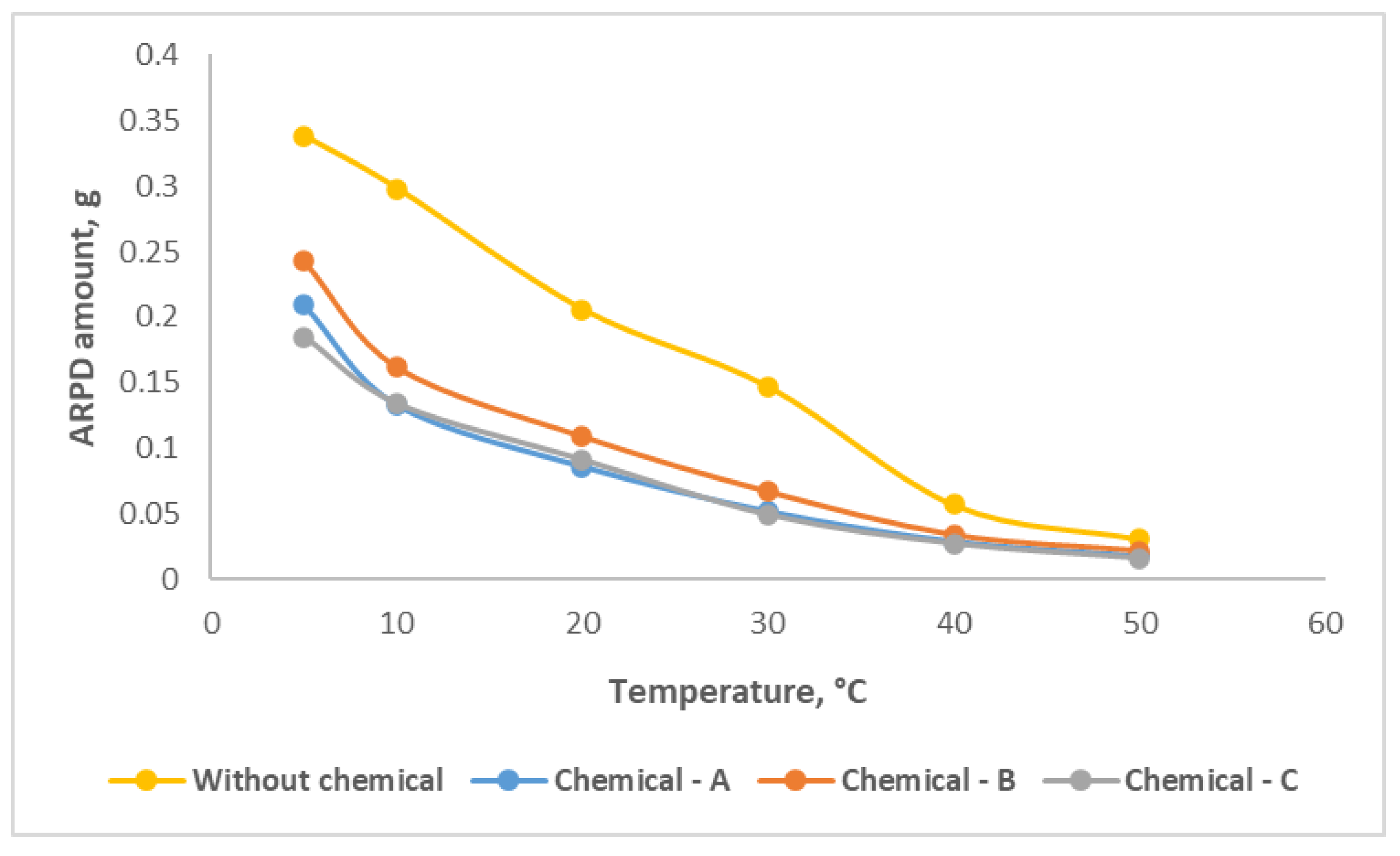
Figure 6.
Effective viscosity change over temperature graph without and with compound chemicals.
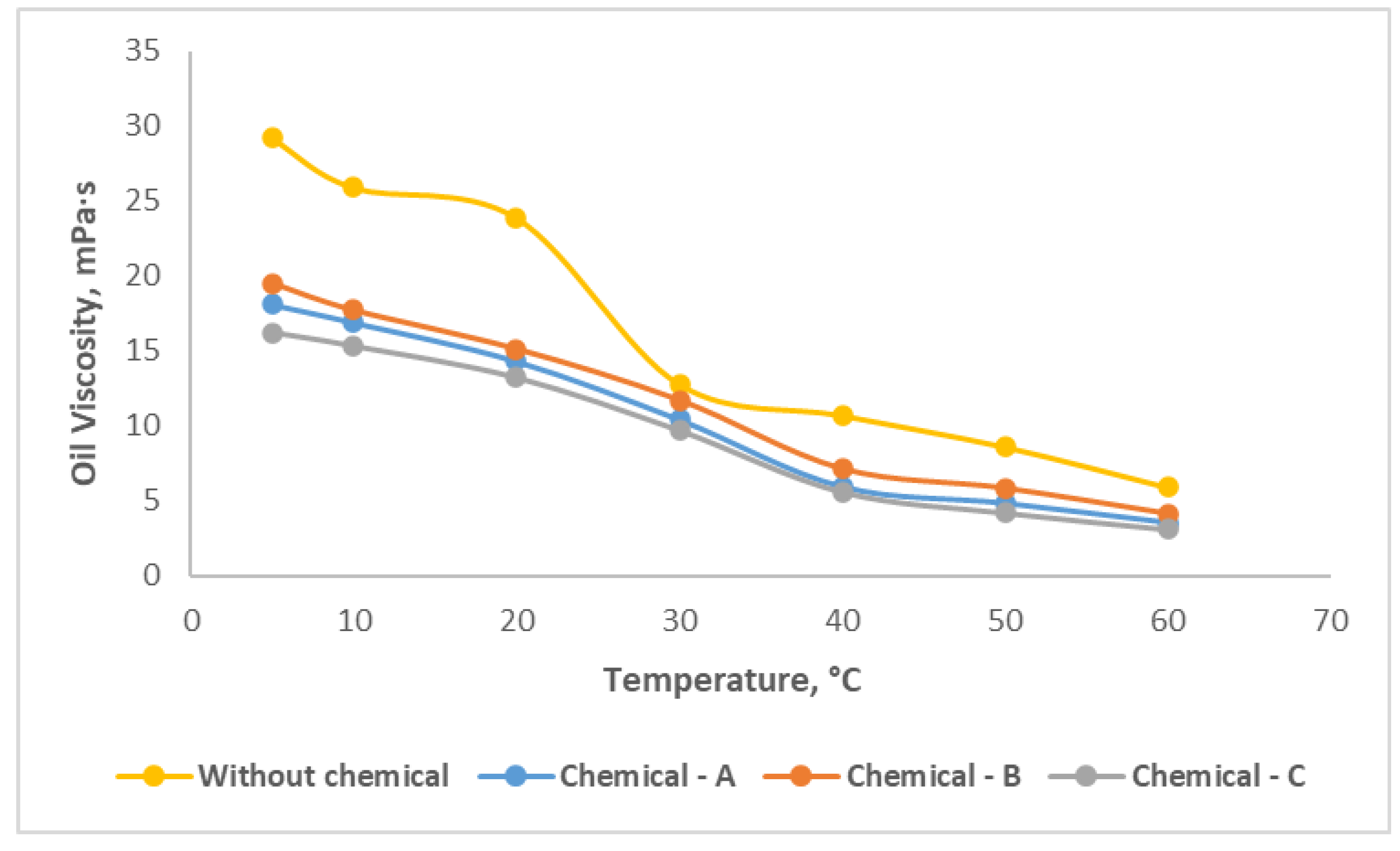
Figure 7.
Corrosion protection effect change over chemical compounds` concentrations.
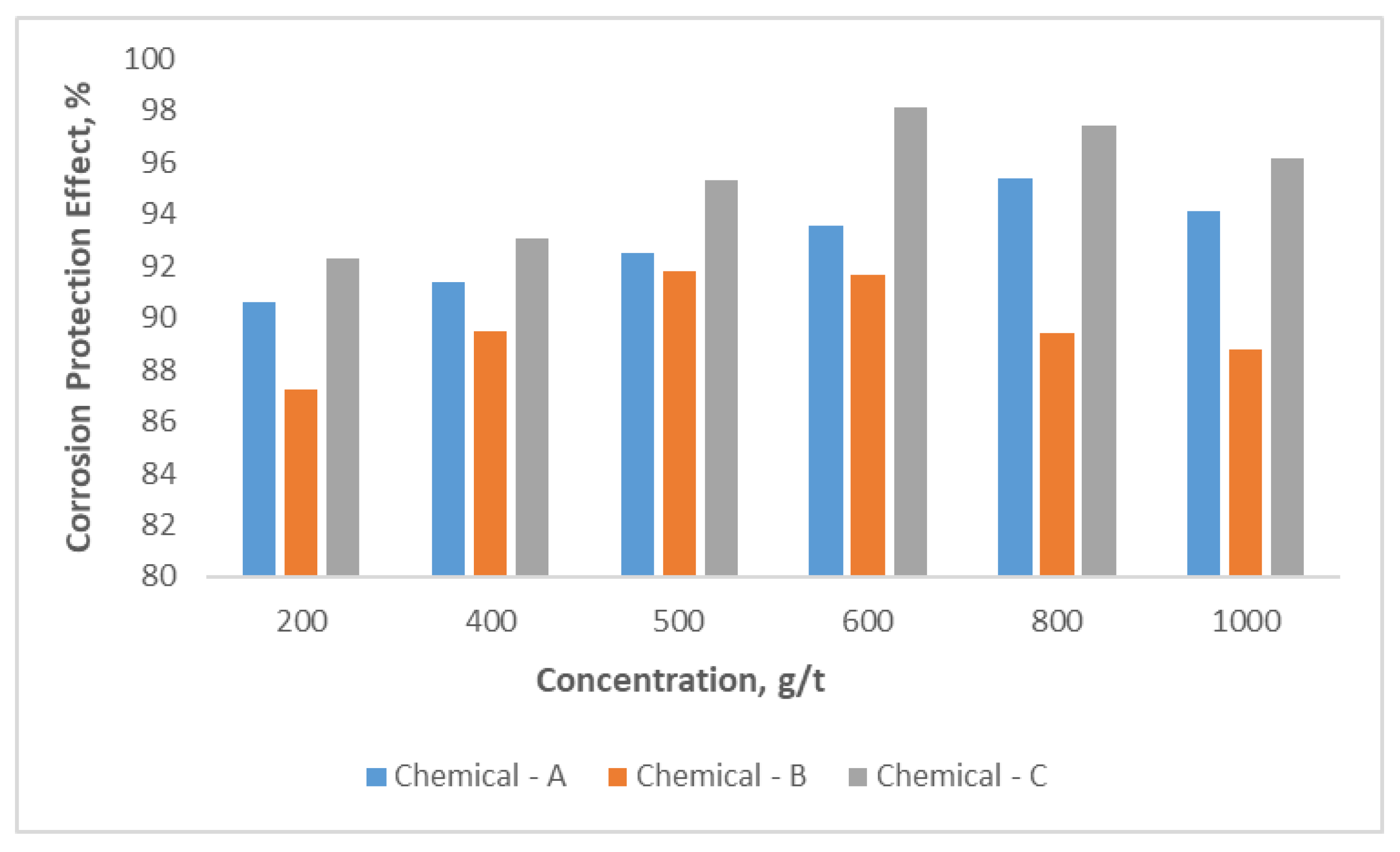
Figure 8.
Oil sample`s pseudo-components.
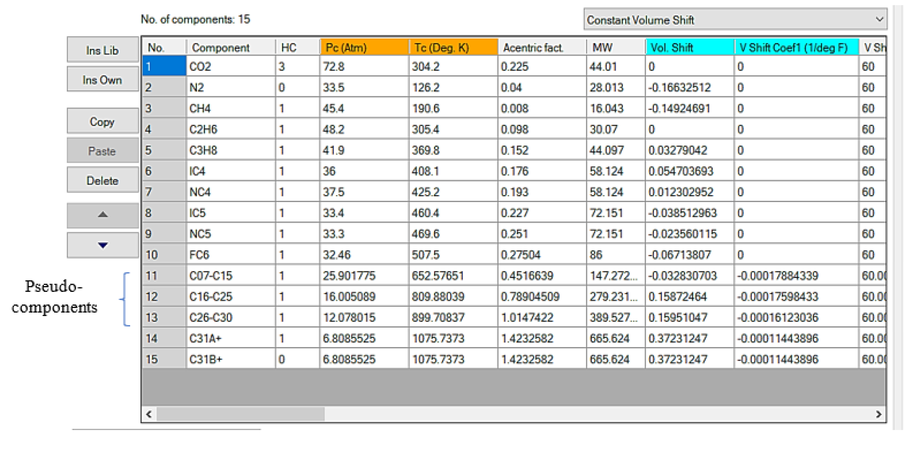
Figure 9.
The asphaltene precipitation curve at 100 °C.
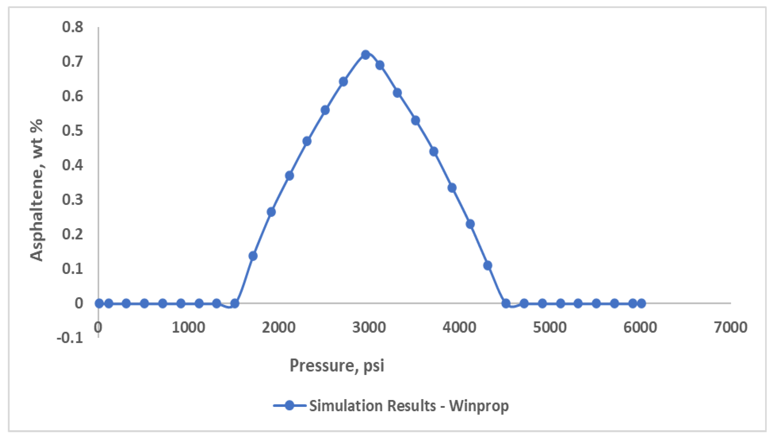
Figure 10.
Simulation model with the producer and injector locations.
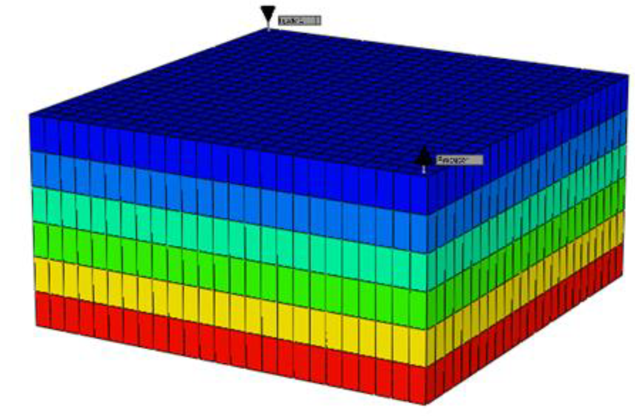
Figure 11.
Recovery factor for the injection pressure with and without asphaltene during waterflooding.
Figure 11.
Recovery factor for the injection pressure with and without asphaltene during waterflooding.
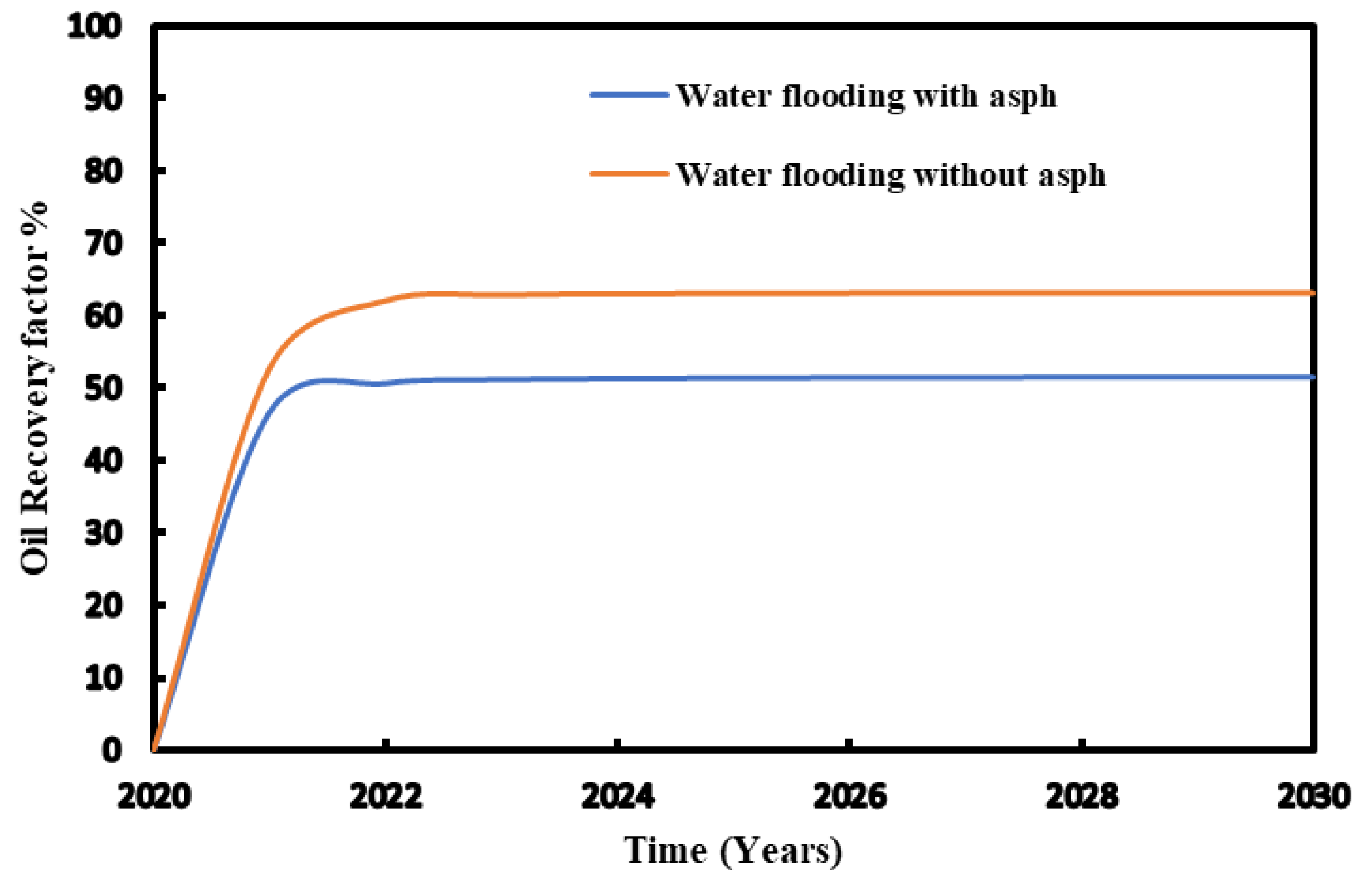
Figure 12.
Asphaltene deposited mass (lb) during waterflooding. (a) start of production; (b) at the end of production.
Figure 12.
Asphaltene deposited mass (lb) during waterflooding. (a) start of production; (b) at the end of production.
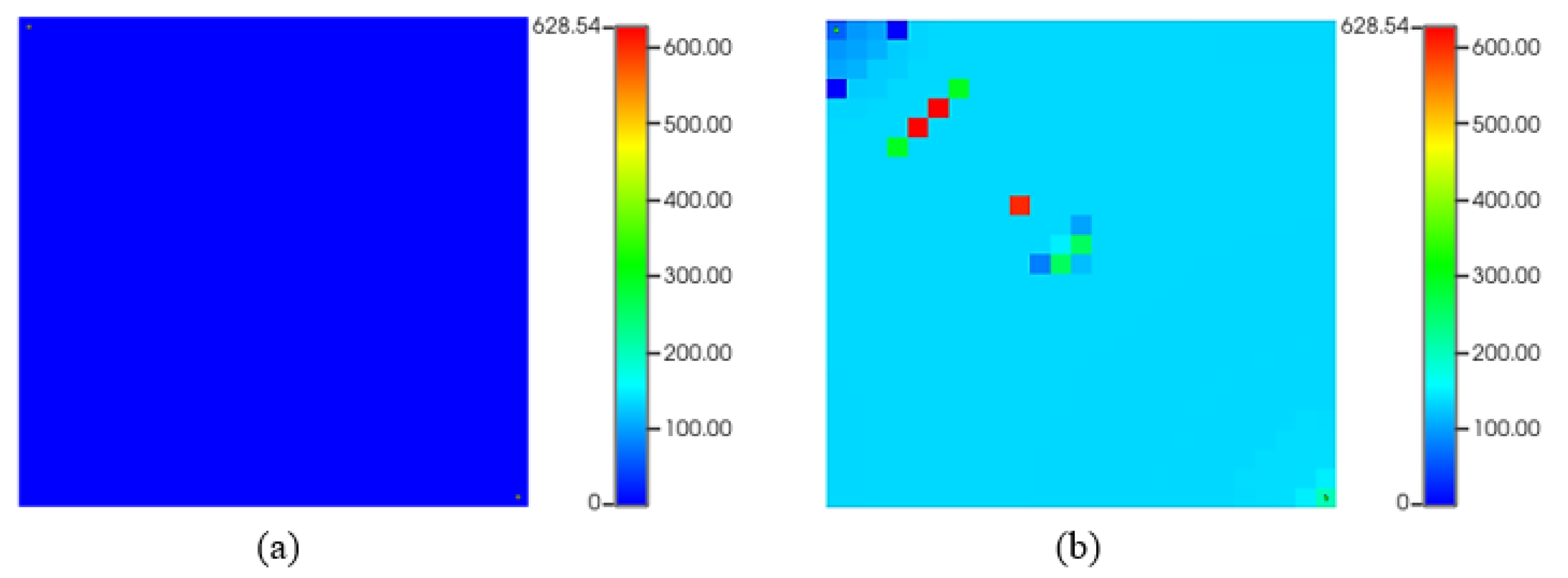
Figure 13.
Recovery factor for the injection pressure with and without asphaltene during CO2 flooding.
Figure 13.
Recovery factor for the injection pressure with and without asphaltene during CO2 flooding.
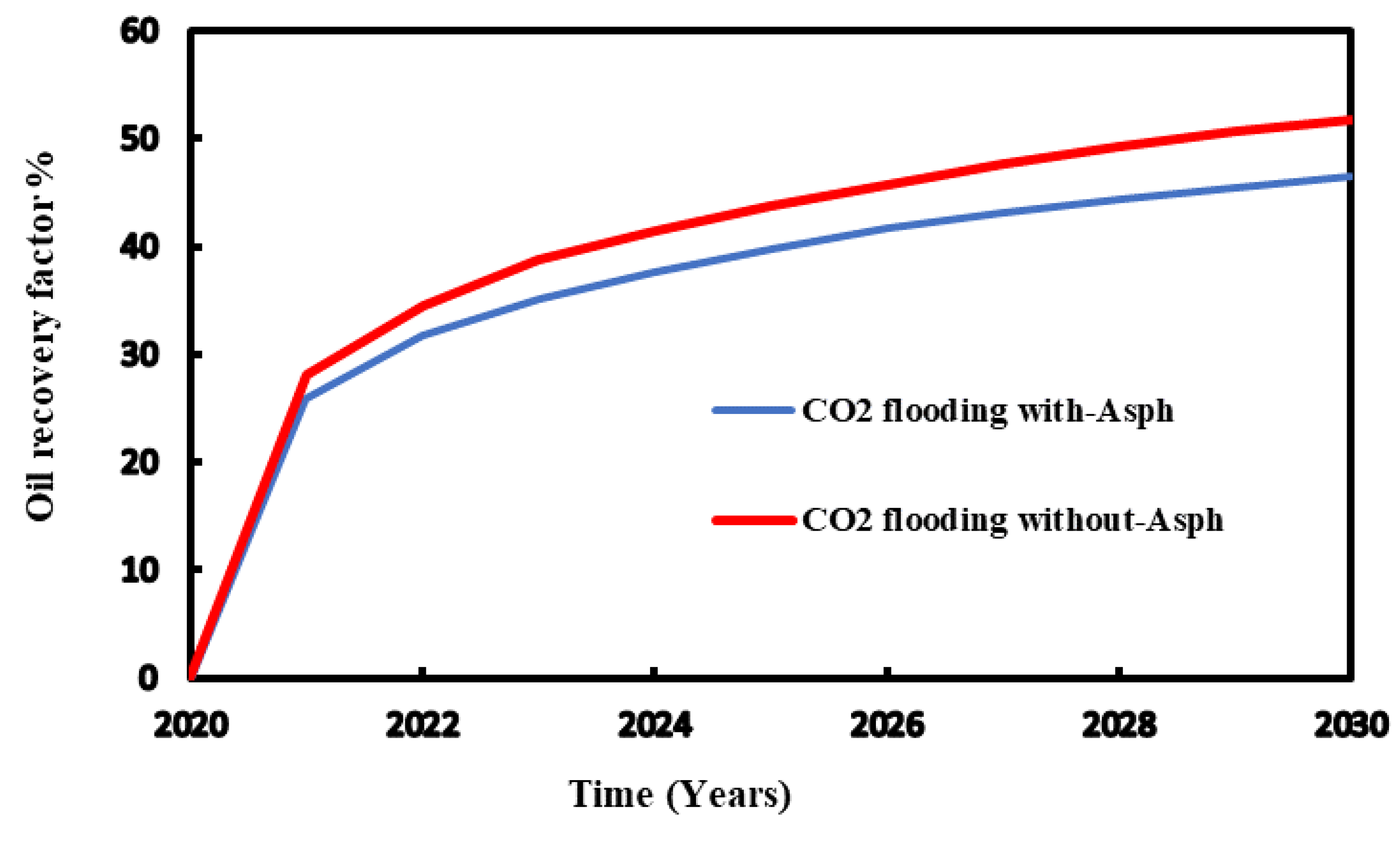
Figure 14.
Asphaltene precipitation (lb) during CO2 flooding. (a) start of production; (b) at the end of production.
Figure 14.
Asphaltene precipitation (lb) during CO2 flooding. (a) start of production; (b) at the end of production.
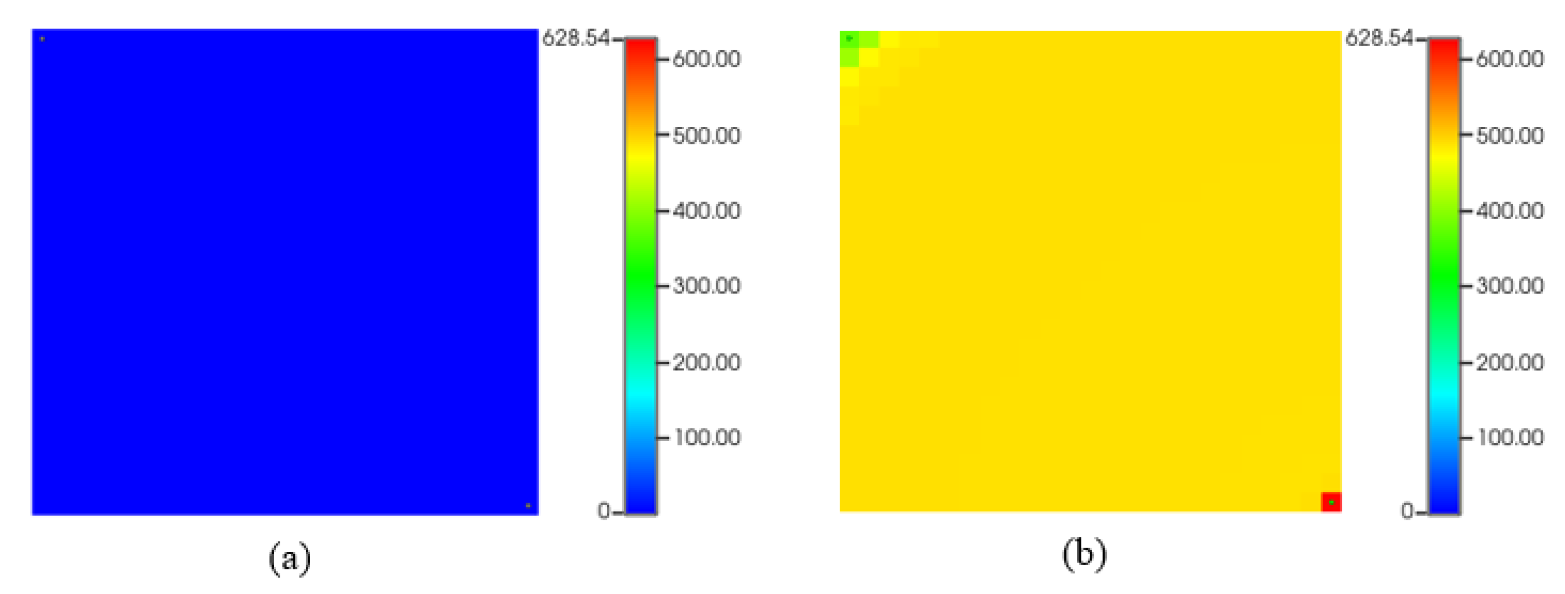
Figure 15.
Recovery factor for the CO2 and waterflooding with asphaltene with reagent.
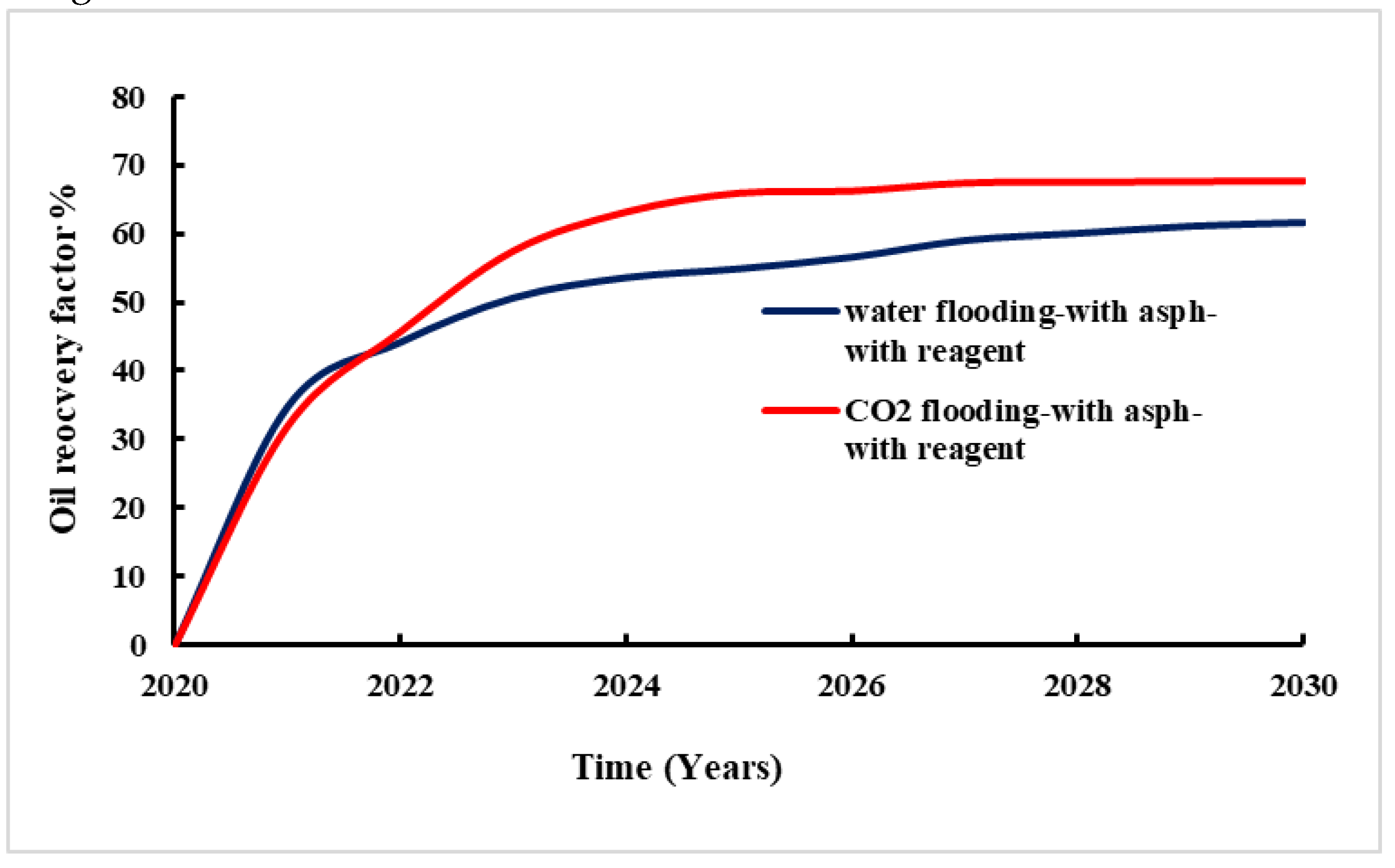
Figure 16.
Asphaltene deposited mass (lb) during waterflooding and CO2 flooding with asphaltene and reagent.
Figure 16.
Asphaltene deposited mass (lb) during waterflooding and CO2 flooding with asphaltene and reagent.
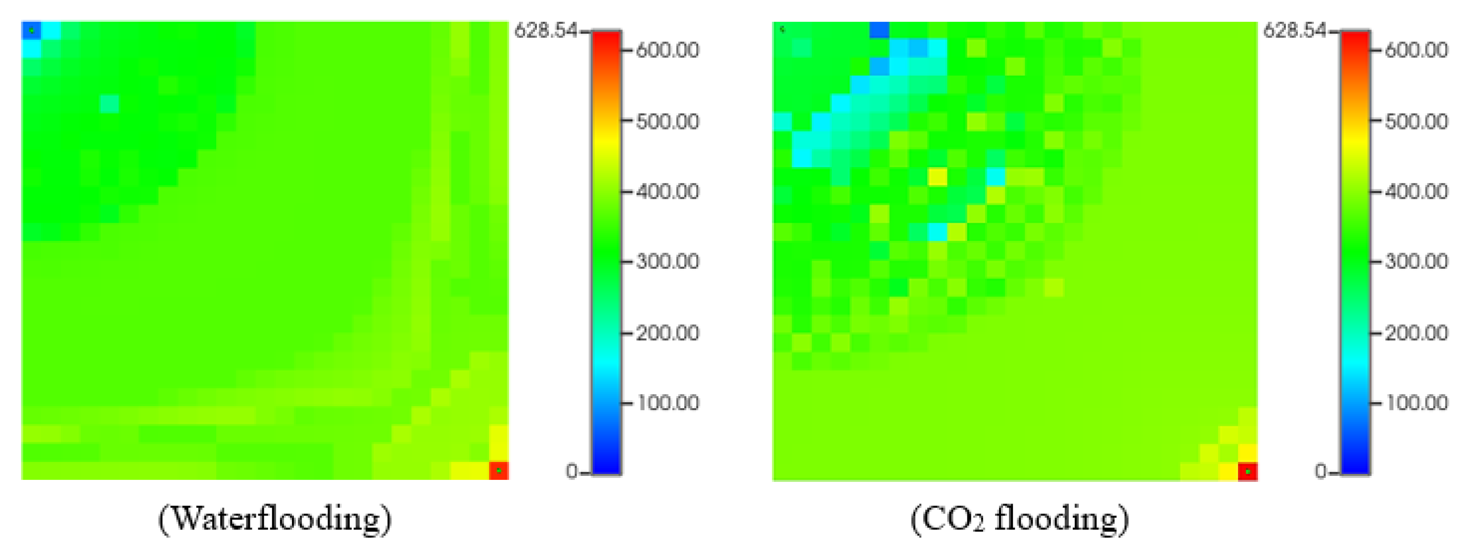
Figure 17.
Oil recovery for waterflooding and CO2 flooding with asphaltene and with/without reagent.
Figure 17.
Oil recovery for waterflooding and CO2 flooding with asphaltene and with/without reagent.
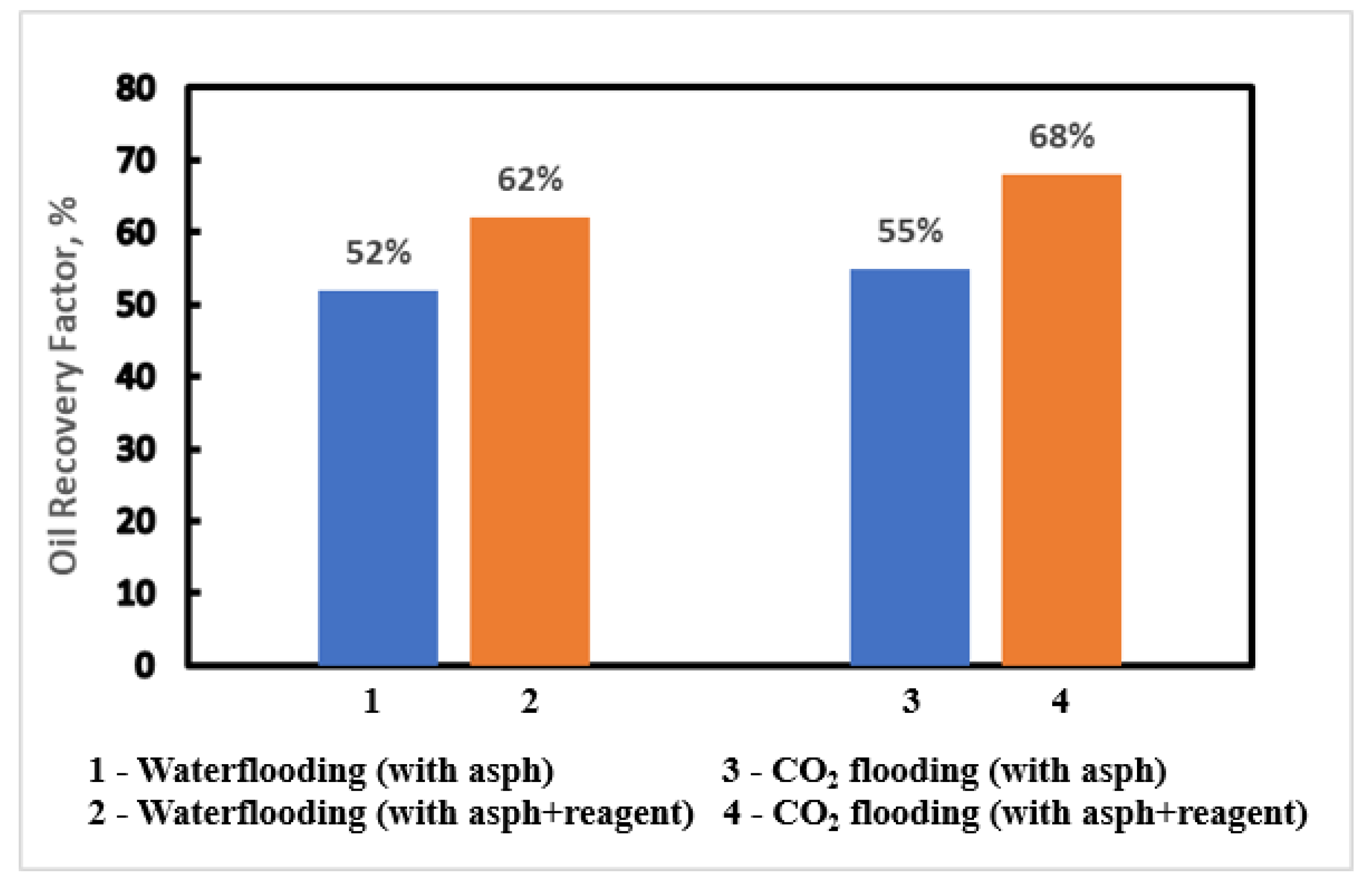

Table 1.
Physicochemical characteristics of “X” oilfield example.
| Content | Paraffin | Asphaltene | Resin | Freezing Point, °C | Water cut |
| Amount, % | 10.23 | 1.84 | 9.18 | +12 | 48.3 |
Table 2.
Chemical composition of Ct20 brand steel (%).
| Brand | C | Mn | Si | P | S | Cr | Ni | Cu | As | Fe |
| Ct20 | 0.17 -0.24 | 0.35 -0.65 | 0.17 -0.37 | ≤0.04 | ≤0.04 | ≤0.25 | ≤0.25 | ≤0.25 | ≤0.08 | 98 |
Table 3.
Effect of chemical reagents on limiting shear stress and non-Newtonian index of oilfield sample.
Table 3.
Effect of chemical reagents on limiting shear stress and non-Newtonian index of oilfield sample.
| Concentration, g/t | Temperature, °C | Limiting shear stress, τ0, Pa | Non-Newtonian index, n | Notes |
| Chemical - A | ||||
| 800 | 5 | 14.7 | 0.63 | non-Newtonian liquid, no flow, solid |
| 10 | 2.91 | 0.82 | non-Newtonian liquid, flow | |
| 20 | 0.082 | 0.94 | non-Newtonian liquid, flow | |
| 30 | 0.044 | 0.98 | non-Newtonian liquid, flow | |
| 40 | 0.0052 | 1 | Newtonian liquid, flow | |
| 50 | 0.0029 | 1.01 | Newtonian liquid, flow | |
| Chemical - B | ||||
| 500 | 5 | 32.2 | 0.55 | non-Newtonian liquid, no flow, solid |
| 10 | 5.51 | 0.72 | non-Newtonian liquid, flow | |
| 20 | 0.14 | 0.87 | non-Newtonian liquid, flow | |
| 30 | 0.067 | 0.93 | non-Newtonian liquid, flow | |
| 40 | 0.0073 | 0.99 | Newtonian liquid, flow | |
| 50 | 0.0059 | 1 | Newtonian liquid, flow | |
| Chemical - C | ||||
| 600 | 5 | 5.51 | 0.79 | non-Newtonian liquid, flow |
| 10 | 1.01 | 0.92 | non-Newtonian liquid, flow | |
| 20 | 0.032 | 0.99 | Newtonian liquid, flow | |
| 30 | 0.011 | 1 | Newtonian liquid, flow | |
| 40 | 0.0028 | 1 | Newtonian liquid, flow | |
| 50 | 0.0009 | 1.03 | Newtonian liquid, flow | |
Table 4.
Physicochemical characteristics of “Y” and “Z” oilfields examples.
| Content | Paraffin | Asphaltene | Resin | Freezing Point, °C | Water cut | |||||
| Oilfield | Y | Z | Y | Z | Y | Z | Y | Z | Y | Z |
| Amount, % | 13.31 | 12.46 | 4.73 | 3.42 | 10.42 | 7.37 | +17 | +16 | 53.6 | 56.2 |
Table 5.
Experimental results of chemical compounds for Y and Z oilfield samples.
| Parameters | Y oilfield sample | Z oilfield sample | ||||||
| Chemical | Chemical | |||||||
| Oil | A | B | C | Oil | A | B | C | |
| Freezing Point, °C | +17 | +1 | +5 | -2 | +16 | +6 | +7 | 0 |
| ARPD amount, g (at 50 °C) | 0.049 | 0.031 | 0.036 | 0.028 | 0.041 | 0.025 | 0.031 | 0.022 |
| Effective Oil Viscosity, mPa·s (at 60 °C) | 8.3 | 5.5 | 6.1 | 4.8 | 7.8 | 4.9 | 5.4 | 4.3 |
| Limiting Shear Stress, Pa (at 50 °C) | / | 0.044 | 0.0076 | 0.002 | / | 0.035 | 0.0066 | 0.0014 |
| Non-newtonian index (at 50 °C) | / | 1 | 0.99 | 1.02 | / | 1 | 1 | 1.02 |
Table 6.
Reservoir Fluid Composition.
| Component | “X1” oilfield sample |
|---|---|
| Nitrogen | 0.0057 |
| CO2 | 0.0246 |
| Methane | 0.3637 |
| Ethane | 0.0347 |
| Propane | 0.0405 |
| i-Butane | 0.0059 |
| n-Butane | 0.0134 |
| i-Pentane | 0.0074 |
| n-Pentane | 0.0083 |
| Heptane | 0.0162 |
| Hexane + | 0.4796 |
| Total | 1.0000 |
| C7+ molecular weight | 329 |
| C7+ specific gravity | 0.9593 |
| Live-oil molecular weight | 171.2 |
| API gravity, stock-tank oil | 19 |
| Asphaltene content in stock-tank oil, wt% | 16.8 |
| Reservoir temperature, °C | 100 |
| Saturation pressure, psia | 2950 |
| Gas-Oil Ratio, scf/stb | 330 |
| Minimum Miscibility Pressure (MMP), psia | 2780 |
Disclaimer/Publisher’s Note: The statements, opinions and data contained in all publications are solely those of the individual author(s) and contributor(s) and not of MDPI and/or the editor(s). MDPI and/or the editor(s) disclaim responsibility for any injury to people or property resulting from any ideas, methods, instructions or products referred to in the content. |
© 2024 by the authors. Licensee MDPI, Basel, Switzerland. This article is an open access article distributed under the terms and conditions of the Creative Commons Attribution (CC BY) license (http://creativecommons.org/licenses/by/4.0/).
Copyright: This open access article is published under a Creative Commons CC BY 4.0 license, which permit the free download, distribution, and reuse, provided that the author and preprint are cited in any reuse.


