
Submitted:
12 July 2024
Posted:
15 July 2024
You are already at the latest version
Abstract
Like many coastal lagoons in several countries, “Navío Quebrado” lagoon (La Guajira-Colombia) is a very delicate and precious environment; indeed, it is a nationally recognized Flora and Fauna Sanctuary. Several factors, amongst which climate change, are threatening its existence because of changes in the governing hydro-morphological processes. A first step to address this problem certainly is to understand its hydrological behavior and to be able to replicate via simulation its recent history and then infer likely futures. These potential futures will be marked by changes in the water input by its tributary, the Camarones River, and by a modified water exchange with the sea, according to a foreseen sea level rise pattern, as well as by a different evaporation from the free surface, according to temperature changes. In order achieve the required ability to simulate future scenarios, data on the actual behavior have to be gathered, i.e. a monitoring system has to be set up, which to date is not existent. Conceptually, designing a suitable monitoring system is not a complex issue and seems easy to implement. However, the environmental and socio-cultural and socio-economic context makes every little step a hard climb. An extremely simple –almost “primitive”- monitoring system has been set up in this case which is based on very basic measurements of current velocity and water levels and a direct participation of local stakeholders, first of all the National Park unit of the Sanctuary. All this may clash with the latest groovy advances of science, like in situ automatized sensors, remote sensing, machine learning and digital twins, and certainly several improvements are possible and desirable. But it has strong positive points: it is providing surprisingly reasonable data and…it is working at almost zero additional cost. Several technical difficulties made this exercise interesting in itself and worth being shared. Its novelty lies in showing how old, simple methods may offer a working solution to new challenges. This humble experience may be of help in several other similar situations across the world.
Keywords:
monitoring
; coastal lagoons
; tidal water exchange
; low-cost technology
; participatory approach
; Colombia
1. Introduction
Peculiarities of Coastal Lagoons
Coastal lagoons are among the most productive systems in the world [1,2]. Indeed, many species take advantage of the lagoons to feed and reproduce, remaining in these places for part of their life cycle. They provide a significant number of socioeconomic benefits for humans who exploit this productivity through fishing [3]. Coastal lagoons are characterized by having little depth, differing greatly in size, morphology, trophic state and salinity characteristics, which conditions the biological structure, species composition and fishing performance [4]. At its lateral limits, the entry of freshwater -typically by rivers- provides hydrological forcing, as does the exchange of water between the lagoon and the open sea [5]. Due to the above, these ecosystems arise great motivation for researchers to study not only their productivity, but also its hydrological and hydrodynamic behavior (inflow, exchange of flows, water levels)
Coastal lagoons are characterized by a typical annual cycle (Figure 1). This usually starts when the feeding river system is flooding thus originating a period of “high waters” where the water level rises until the natural sand bar that separates the lagoon from the open sea breaks down so creating an open mouth (“la boca”; in some case, local inhabitants contribute to artificially open it to avoid flooding of their houses). In these conditions, the outgoing flow of semi fresh water is felt by sea populations of fish (for Navio-Quebrado: Litopenaeus schmitti, Macrobrachium acanthurus, Centropomus undecimalis, Elops saurus, Micropogonias furnieri, Mugil curema, Mugil incilis, Mugil liza, Cathrorops spixii and Eugerres plumieri lito, Mugil liza, Mugil curema ) and crustaceous which hence enter the lagoon looking for appropriate zones for reproduction and nursery. While the river fresh water input reduces (and often remaining null for several months), the lagoon volume reduces and during a few months an alternate flow exchange of water into and from the sea is established, according to the tidal pattern. In this period the fingerlins and grown fish take advantage to exit and look for freedom and a new life into the open sea. This goes on until the sea waves prevail on this exchange process and recreate a sand bar, so closing the boca. From this moment on, until the next cycle starts, the lagoon water evaporates, lowering its level (depth) and its area, while salinity strongly increases. All the fauna trapped inside is destined to die because of hypersaline conditions, unless a new flood timely comes. Referring to Navio-Quebrado, curiously local fishermen collect this dead or dying biomass -mostly composed of Elops saurus followed by mugilids [6]- as a delicious, although stinky, food (named “cachirra”, by the natives of the area).
2. Methods: Practical Challenges and Adopted Solutions to Set up a Monitoring System for Camarones Lagoon
A hydrological monitoring system, aiming at feeding a hydrological model (water balance), for a coastal lagoon should include at least the following:
- a)
- Fresh water inflow by the Tomarrazón-Camarones River (tributary), what implies measuring its discharge in a station sufficiently close to the lagoon to represent the whole water basin supply, but at the same time sufficiently far to be influenced by the backwater effect as little as possible.
- b)
- Storage and release flows from changes of water volume stored in the lagoon. This implies being able to measure the level of its water surface and to know the morphometric relationships linking such level to the stored volume (and surface area)
- c)
- Salty or brackish water exchange lagoon-sea (only when the boca is open), as this may be a key component of the water balance. Measuring this variable is not easy, but for the systematic monitoring, the idea is to measure essential variables, namely the water surface elevation of the lagoon and of the sea, and to derive a relationship linking them to the exchange flow.
- d)
- Fresh water inflow from precipitation directly falling on the lagoon itself and from runoff from the local watershed into the lagoon. Both can be estimated from measurements of the precipitation in close-by sites and the area of the two components (local water basin and lagoon); but the first one requires some rainfall-runoff relationship (model)
- e)
- Evaporation losses from the water surface of the lagoon: this can be calculated from direct estimates of evaporation rates or from indirect estimates based on formulas where the measured variables would be temperature, humidity and the like.
Filtration exchanges with the sea and nearby area can be neglected at first as the bottom of the lagoon is considered to be basically sealed by fine sediments (silt and clay) and the water head potentially able to generate a filtration with the sea is very low, while the potential zone of exchange (mouth) is quite limited.
The physical system is shown in Figure 3 together with key elements.
It is spontaneous to think of a (possibly low cost) technological system to measure several of such variables. Low-cost systems are in general modular, thus allowing for an easy replacement of damaged parts. Modularity also allows for a wide freedom in the selection of components, from the sensors, recorder, measurement algorithm, communication technology, feeding source and other characteristics [15,16,17]. These systems are suited for a variety of contexts: e.g., water quality monitoring (nutrients, dissolved oxygen,..) in a river [15]; environmental monitoring: aquifer level, air quality, sediments, or the dynamics of wind transported sands [16]; management of urban waters [17] measurement of water level in a river [18]. We hence evaluated at first this possibility for the different components of the sought system
2.1. River Inflow
No gauging station exists on the Tomarrazón-Camarones River; therefore, the first idea was clearly to set up a new, low-cost monitoring station of the river stage h with automatic measurements (by a pressure or distance sensor) and possibly tele-transmission of data [18,19], and in parallel set up a suitable stage-discharge relationship Q(h), analogously to what has been done for example by [5].
Unfortunately, our experience in the area led us to immediately discard this idea considering the high probability (better said, the certainty) of rapid robbery or damage of the devices: very poor people are prone to steal anything can reward them with even less than a dollar.
Another option was to adopt satellite measurements of water levels via sensors like (TOPEX/Poseidon, Jason-1, 2, and 3, ERS-1/2, Environmental Satellite (Envisat), ICESat, CryoSat-2, SARAL/AltiKa, SWOT with the support of software like AlTiS [20]). But, analogously, this option was discarded for several reasons: the channel is almost invisible from above owing to the riparian vegetation cover; the channel is too narrow (10-20 m) ; the frequency of survey of satellites is too low for our purposes. These tools however have produced data during two decades that can be very useful to study for instance the evolution of water bodies [21,22,23,24].
As the rainy season about to start at that moment, and missing it would be a significant data loss, a very simple, but robust and even economic solution was set up. A rule was painted on a fixed vertical wall part of the foundation pillar of a bridge. Actually, two rules were set up in the only two bridges existing in the area (Figure 3b): Puente Troncal, the one selected for the routine measurements, and Puente Viejo. This was done to perform a check on data coherence, as well as on the existence of a backwater effect, and to provide an alternative calculation of flow based on the gradient of water level (as explained later). Details of the rules in both bridges can be observed in Figure 4.
The selected cross sections are sufficiently stable because the riparian material is mainly an organogenic claystone conglomerate, although of course a certain level of sediment deposits change may take place. With a survey during dry conditions, we determined the geometry of the cross section so that the relationship A=A(h) was obtained where A is the area of the wet cross section for water level h (Figure 5).
To simplify as much as possible the routine measurement process, we ensured that the water surface and the rule were visible in any condition from a selected site on top of the bridge and opted for just taking a picture ideally a couple of times each day at (more or less) fixed times (early morning and mid-afternoon). Providentially, we could arrange a formal agreement with the local National Parks office that immediately and enthusiastically shared the necessity of setting up such a project and accepted the pledge to have one of its staff members passing by the site and taking the picture. In addition, we made a private agreement with a local person (“muchacho”) with a motorcycle who, under a very reasonable payment, would commit to “echar un ojo” (have a look) of the river every day and who, in occasion of a flood or an emergency (e.g., the impossibility of Parks servant to pass by), would take an additional picture registering the time and immediately sending it to us by WhatsApp®.
Still the second part of the problem had to be faced: setting up a stage-discharge relationship. This meant gauging the flowrate particularly during high flows, a quite dangerous task. The use of a classic current meter was out of discussion because the bridge is too high over the water to hold the device with a long rigid arm, while an ADCP (Acoustic Doppler, Current-meter Profiler) would require to access the water body during high water and that was physically very hard and dangerous owing to the dense vegetation one should cross and the slippery ground (Figure 6); in addition -and most important- our University simply had no such device yet. On the other side, wading the river would certainly be impossible because it becomes very deep and fast with a slippery bottom, while in low water wading would interfere with the flow we had to measure. Other methods like salts concentrations or dyes were not viable because again of the impossible access and because that river feeds a nature protected area. This is why we chose the old, somehow “primitive” method of throwing a floater and measuring the time elapsed to cover a fixed, known distance (of 11 m), and averaging amongst several (at least 3) launches along different flow lines across the section. Only biodegradable objects, like fruits (ideal because they float, but almost fully immersed so the wind effect is minimal) or short wood sticks were used. The flow rate was then obtained by just multiplying the average velocity obtained times the area of the wet section determined based on the water level h and the known geometric section A=A(h) previously determined in dry conditions (from Figure 5). No correction to the velocity for border effect was applied because the velocity field is quite complex and sometimes the main flow occurs on the side rather than in the central sector.
Definitely, this approach appears to most readers, as to us as well, quite anachronistic and primitive. Nevertheless, the obtained data after more than one and a half year of observations behave surprisingly well as shown in Figure 7 (interpolated by a polynomial regression equation).
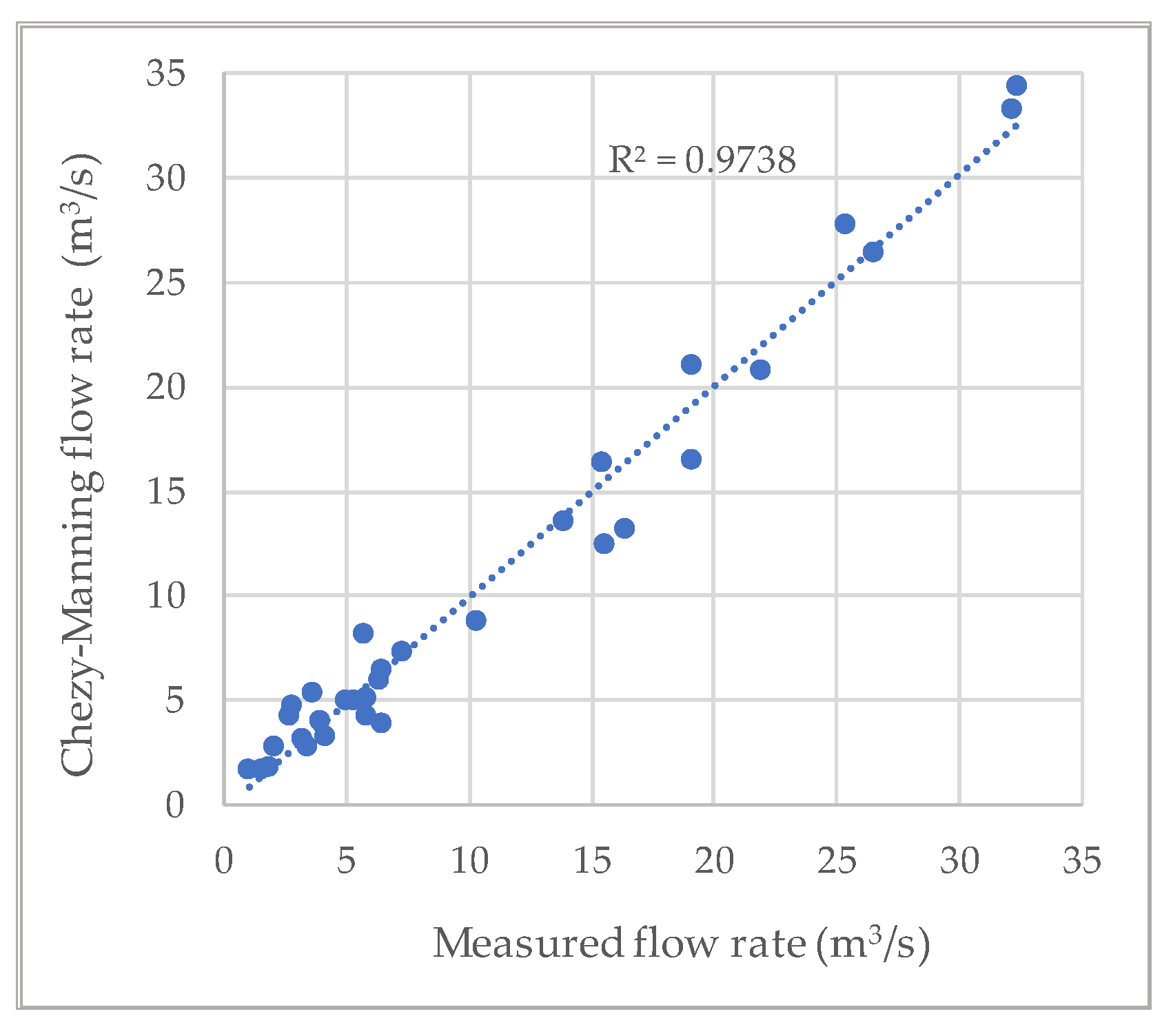
To confirm this quite positive result, and for scientific curiosity, a different method to estimate the flowrate based on classic hydraulics, that is by applying the Chezy Manning’s equation 1 [25], was adopted, being it often used in current research (e.g., [26,27,28]), here we used the area A=A(h) and wetted perimeter p=p(h) relationships obtained from the cross section geometry of Figure 5 by points (Figure 8), and for the slope s [m/m], for each measurement (at a given date and time), the water elevation difference Δy between the two bridges monitored (yT at P.Troncal and yV at P.Viejo, see Figure 3) divided by their distance L along the stream axis (L=1132 m from Google Earth® image), was used, once established a reference elevation for both (the “IGAC 0”; with IGAC: Instituto Geográfico Agustin Codazzi, the official Colombian entity in charge of geographical issues and maps), so transforming the water depth h of our hydrometer into an elevation y. With this position, the stage-discharge curve at P.Troncal station as shown in Figure 9, was obtained, by estimating the Manning friction coefficient n from manual trial and error to fit the measured values as far as possible (getting the value n=0.0447 in the SI system). Again, results are surprisingly nice, as demonstrated by Figure 9. Nevertheless, for the monitoring exercise the empirical stage-discharge curve (based on our measurements) is preferred simply because this is closer to reality and because more data will be available in time making it little by little more reliable.
v(h) = 1/n * R(h)2/3 * s1/2 (1a)
with:
Q(h)=V(h)*A(h) (1b)
v [m/s]: average velocity in the cross section
Q [m3/s]: flow rate
h [m]: water depth in the section
A [m2]: area of the wetted cross section
R [m]: hydraulic radius, that is: R(h)=A(h)/p(h)
s [-]: the river slope
p [m]: wetted perimeter
y [m.a.s.l]: water elevation: y=h+h0 with h0 IGAC reference [m.a.s.l].
Figure 8.
Analytic relationships (approximated) for P.Troncal cross section of the river: a) wetted area A=A(h); b) wetted perimeter p=p(h).
Figure 8.
Analytic relationships (approximated) for P.Troncal cross section of the river: a) wetted area A=A(h); b) wetted perimeter p=p(h).
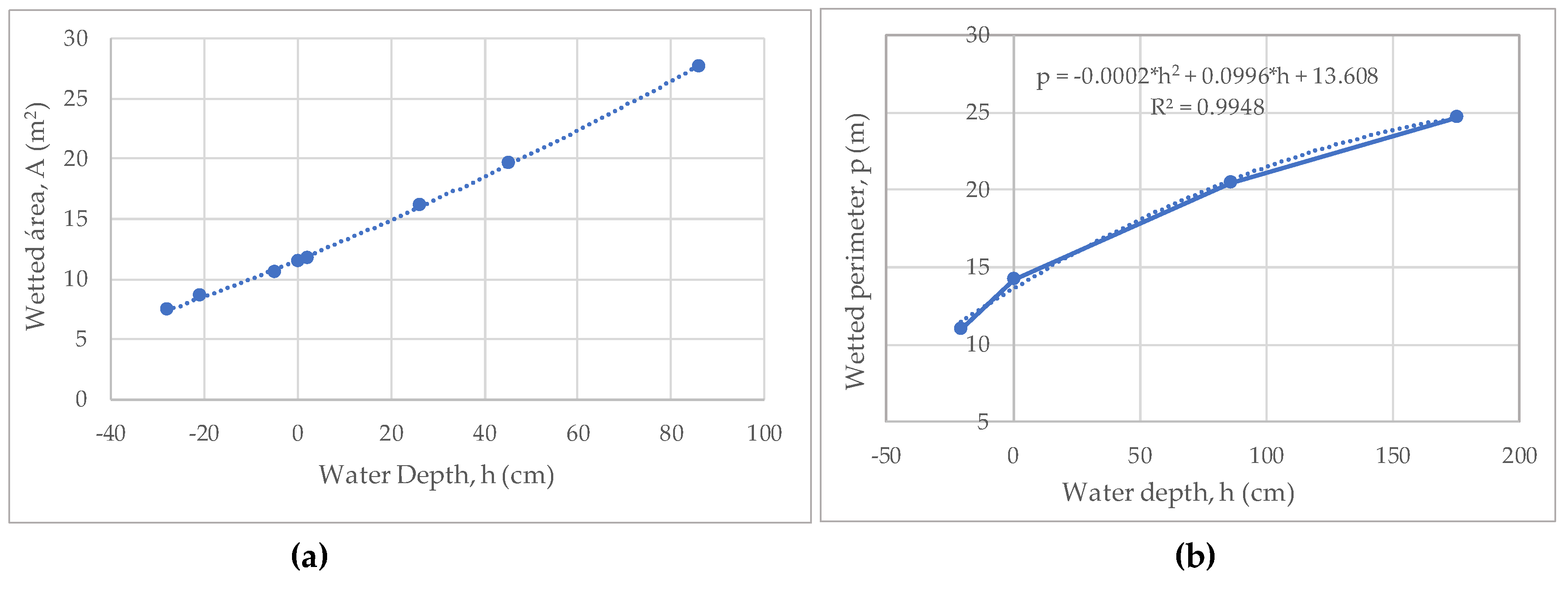
Figure 9.
Matching between measured Q and Q estimated via Chezy-Manning equation (R2= 0,9738), with data from 23 April 2022-23 October 2023.
Figure 9.
Matching between measured Q and Q estimated via Chezy-Manning equation (R2= 0,9738), with data from 23 April 2022-23 October 2023.
Novelties
But things never are as smooth as they appear at first sight. While the data collection process was going on, we updated the exercise done after an additional month (November 2023) when new significant flood events took place. Figure 10 shows the stage-discharge curve with the new data showing a significantly worse behavior, although still not bad.
The suspect arose then that the deviations detected in the stage-discharge curve of Figure 10 could depend on the backwater effect from the lagoon. Indeed, Figure 11 plotting the flow rate deviations (Q measured-Q estimated by the empirically found stage-discharge relationship) as a function of the water surface level of the lagoon, shows a certain tendency to over-estimate Q (i.e., a negative deviation), for increasing values of the water elevation in the lagoon (i.e., towards the right), as expected.
We therefore sought to improve the found power-law relationship by incorporating a dependency on the water elevation in the lagoon yL, i.e., Q=Q(yT, yL); specifically, a relationship with a term that would reduce the flow value Q for a lagoon elevation yL closer to the river stage elevation yT at P.Troncal (always higher than yL), was set up, as shown by Equation 2a that simply expresses mathematically this concept. Its four parameter values have been calibrated by trial and error (y in [cm.a.s.l]):
Q = a (yT – y0)b [1 - 1/eθ( yT – yL)] [m3/s] (2a)
where the parameters “a, b, y0 and θ“ were determined via calibration and assume the following values are (equation 2c):
a = 0,13299; b=1,00927 (2b)
y0 = -1,900; θ= 0,02600 (2c)
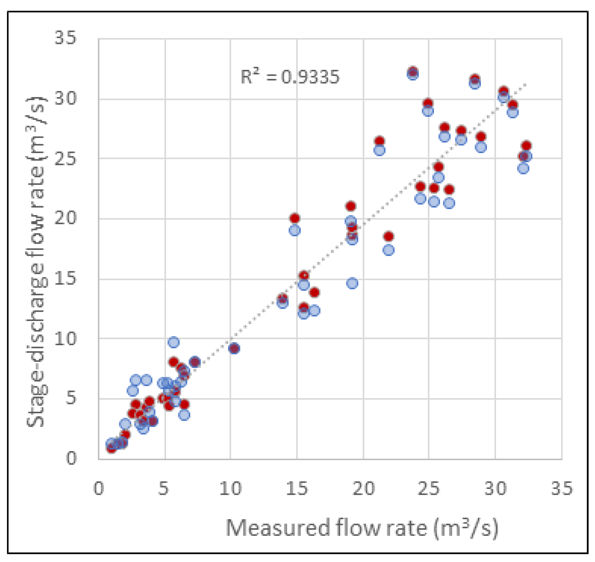
The result is shown by the corresponding matching graph (Figure12) where a certain improvement is apparent both in terms of a closer position of the linear tendency line to the perfect matching line (solid red, 45 degrees) and in terms of dots closer, in general, to that line (indeed R2=0,9335 overcomes the value obtained by the mono dimensional regression, Figure 9). The improvement, however, is more relevant for low values of Q; but this is clearly reasonable as the backwater effect of the lagoon vanishes for high flows as they are associated to high stage while the lagoon water elevation moves in a quite limited range. It is certainly possible to better calibrate the set of parameters and even to find better functional relationships; but for the moment this is the stage-discharge relationship adopted herein after.
Figure 12.
– Improvement of the matching between measured Q and Q estimated by the Q=Q(yriver, ylagoon) relationship (light blue dots are the same as in Figure 9 for ease of comparison). Data until 23 November 2023.
Figure 12.
– Improvement of the matching between measured Q and Q estimated by the Q=Q(yriver, ylagoon) relationship (light blue dots are the same as in Figure 9 for ease of comparison). Data until 23 November 2023.
2.2. Sea: Level
The sea level is a fundamental variable because it determines the exchange relationship between the lagoon and the sea according to tides and the status of the mouth and, as such, it governs the annual life cycle of the same lagoon.
At first, the idea was to install a dedicated sensor to measure water level with high frequency (as reported for instance in [29]), but this idea was immediately discarded for the same security reasons already explained and also for the absence of a suitable installation site. A much simpler solution was hence adopted by simply using existing reported sea level data; in our case, the tide gauge at Puerto Brisa (see Figure 1, a) located 39 km away from the mouth of the lagoon is the closest one.
Getting those data -which are collected and owned by DIMAR (Colombian Dirección General Marítima y Portuaria)- is however a process that requires administrative steps and time, as hourly data are not available on line; hence data are obtained always with a delay of a few months, under explicit request. Another difficulty is data format: on the one side, they are delivered partly with a date dd-mm-yyyy format, and partly with a mm-dd-yyyy format. A harsher difficulty is creating, within a continuous, hourly (Excel®) data record sheet, an automatic reference to other sheets where our discontinuous-time data of measurements of river flowrate&level, measurements of the lagoon level (usually bi-daily between 7-9 am and 4-6 pm, but with exceptions) and area of the mouth & lagoon-sea exchange flow rate were recorded (by transcription of the physical field data formats): these data are collected at different, irregular times with many missing data (“holes”). To deal with this situation, we developed a specific Excel spreadsheet with suitable algorithms that proved to be indispensable, although far from trivial.
But another, more serious problem concerned the altimetric consistency of data. According to the common sense, the tide should oscillate most of the time around the 0 with positive and negative values, although periods of higher or lower moving averages are well possible due to particular combinations of the astronomic drivers and the meteorological ones. But here almost all of the sea elevation data appeared well higher (about 60 cm) than the topographic IGAC 0 (Figure 13), what is impossible because in those conditions no flow from the lagoon to the sea could occur, while it is clearly physically expected and was indeed observed in the field. We then asked formal explanations to the entitled institutions (DIMAR, IGAC, IDEAM- Instituto de Hidrología, Meteorología y Estudios Ambientales) and could understand that that tide-gauge, as the whole Colombian national geodesic network managed by IGAC, is referenced to a 0-sea level located in the Pacific coast in Bonaventura town, which is a completely different water body and indeed the average sea level in the Caribbean -where Puerto Brisas and Camarones are located- is in general 28 cm lower (in [30,31]). But this fact does not solve the mismatching as both the river elevation and that of the lagoon are referred to the same IGAC 0 and as such should be consistent. The final explanation is hence that a deviation exists between the geoidal and the ellipsoidal models of the Earth surface in Colombia as at present there is no official update of the Colombian model. This is indeed consistent with the results found by [32] when trying to validate geometric levelling points with classic topography and LIDAR data finding an average difference of 0,63 m.
In order to proceed, it was therefore assumed that P.Brisa tide-gauge utilizes a different (unknown to us) local reference and without searching for that datum, the mismatching was solved by adopting a very operational criterion: as will be detailed in a forthcoming paper, we just imposed that the lagoon-sea flow exchange process were physically meaningful, that is, when the observed flow was outgoing (from the lagoon into the sea), the lagoon water elevation should be higher than that of the sea, and vice versa. Luckly, a meaningful value of a fixed vertical translation of the tide-gauge data could be found by trial and error that which could fulfill this condition in all observed cases, except just one. Considering that just a tiny level difference (few centimeter) is involved, and that the tide-gauge is 39 km apart and that there are often strong winds, the obtained result can be considered fully satisfactory.
2.3. Lagoon: Water Level
The most spontaneous solution for the measurement of the water elevation of the lagoon seemed to be the installation of a rule fixed at a pole in a quite centric place in the lagoon so that even for low levels the rule would be still immersed (as the lagoon is quite shallow and the bottom characterized by a very gentle slope); and the measure would be taken by the personnel of National Parks from there headquarter on the shore by using a binocular. But this idea was soon discarded because the reflection of the sun light on the water would make remote reading impossible and because wind, the perennial companion of sunlight, generally provokes a high frequency, irregular wave system with amplitude of about 5-15 cm with would severely affects the measures. Even an automatic sensor –that might allow a certain degree of digital filtering of data- was discarded because of the usual security problem and in line with the idea to create a very basic system.
Therefore, a manual device installed at the Parks headquarter located on the lagoon shore (Figure 1 for general location and Figure 14) was chosen.
It is licit to wonder whether the foreseen monitoring frequency of twice a day is sufficient to capture the lagoon dynamics. According to Shannon [33], in a linear (linearized) dynamic system, sampling should be carried out with a frequency not lower than T/10 where T is the min time constant. This criterion, as will be explained in a forthcoming publication, leads to a very wide range of values; specifically, when the mouth is open, the criterion provides values of 1.6 to about 5 hours (depending on the filling status of the lagoon, being quicker when it is low); when the mouth is closed, and the core dynamics is governed by evaporation, it ranges from a couple of days to two or three months. Evidently, only in this second case our monitoring is definitely adequate, while, when the mouth is open, our measures cannot capture the full oscillations process, which is tuned to tide oscillations. Nevertheless, the data obtained can be very informative, as shown in the rest of this paper.
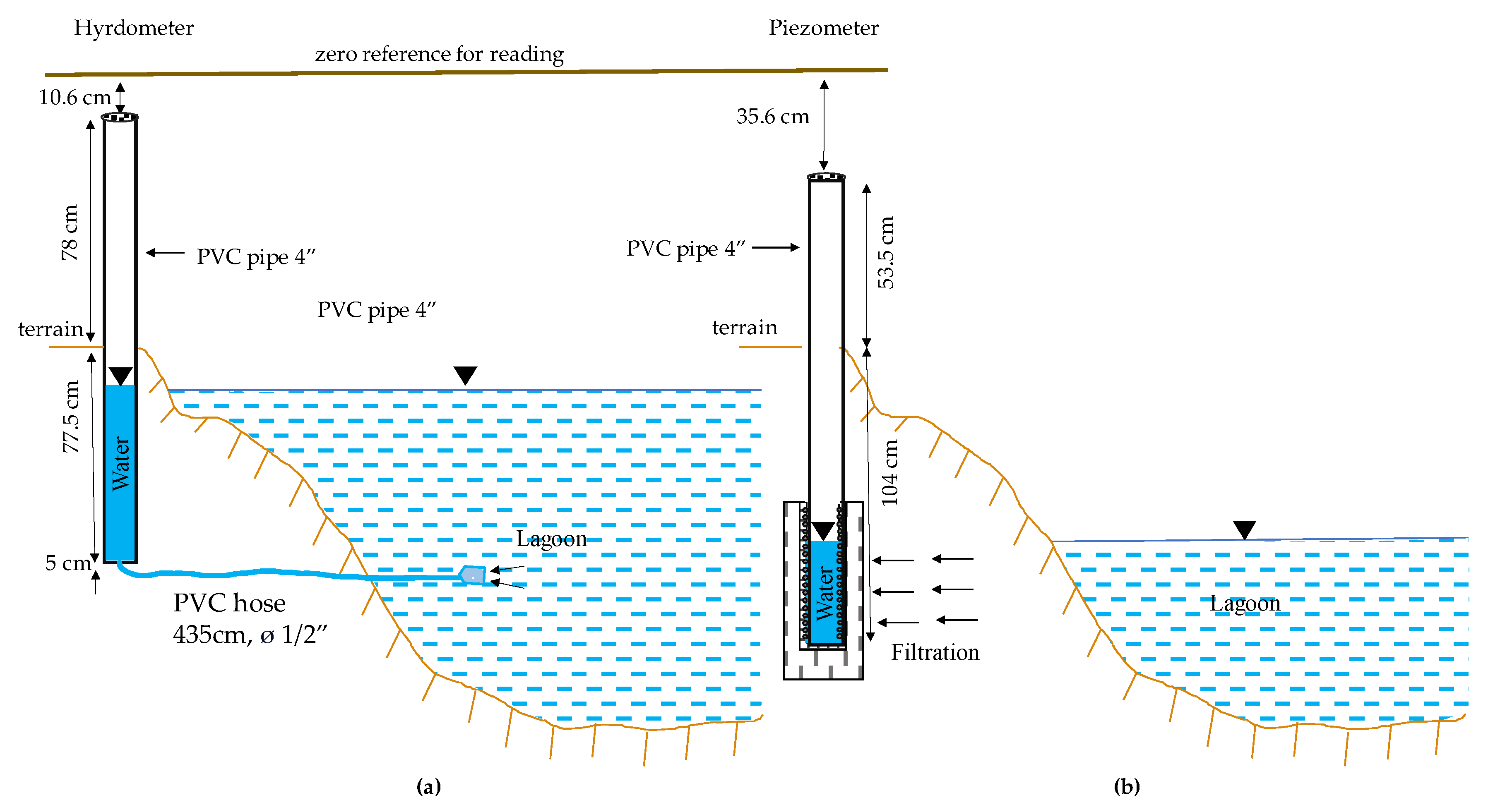
A mixed solution was therefore preferred: a hydrometer (Figure 15a) on the shore, to be used for medium-high levels and a piezometer for situations with lower levels and therefore dry hydrometer (Figure 15b). As water levels can go lower than the local terrain, the hydrometer is enclosed in a typical yellow sewerage pipe set in vertical position and the reading is done by inserting manually a rule, reading indeed the depth with respect to a horizontal reference set on the headquarter structure as indicated. To avoid the disturbance from the high frequency wave oscillations, the device has a feeding tube with a reduced section of diameter Φ = 1.27 cm (which allows only a very small flow to pass through according to the change of head from the lagoon surface local, vertical movement), while the main vertical pipe section is proportionally much larger (Φ = 7.62 cm) so that the water volume input because of a flow increment translates into a much smaller vertical change, so fulfilling the dampening effect (“low-pass filter”). This function, on the other hand, is intrinsically guaranteed for the piezometer as the seepage across the soil cannot accelerate significantly, but, on the opposite side, can dampen frequent (hourly) oscillations. The important difference is that water enters the hydrometer through the tiny tube, directly governed by the head on top of it, while water enters the piezometer by direct seepage across the soil matrix around it; therefore, the former cannot provide a reliable datum when the lagoon level drops below the sucking tip of the tube; while the piezometer works improperly when the level overcomes the ground level and even more when it pours into the pipe from the top of the device.
The implementation of the devices is based on “home-made”, very low cost, technology, as shown in Figure 16).
Figure 15.
Construction details of the water surface measurement system: (a) sealed inlet of the hydrometer; (b) filtering lateral Surface of the piezometer covered by a plastic grid and inserted in a gravel filled holes; (c) full installed system.
Figure 15.
Construction details of the water surface measurement system: (a) sealed inlet of the hydrometer; (b) filtering lateral Surface of the piezometer covered by a plastic grid and inserted in a gravel filled holes; (c) full installed system.
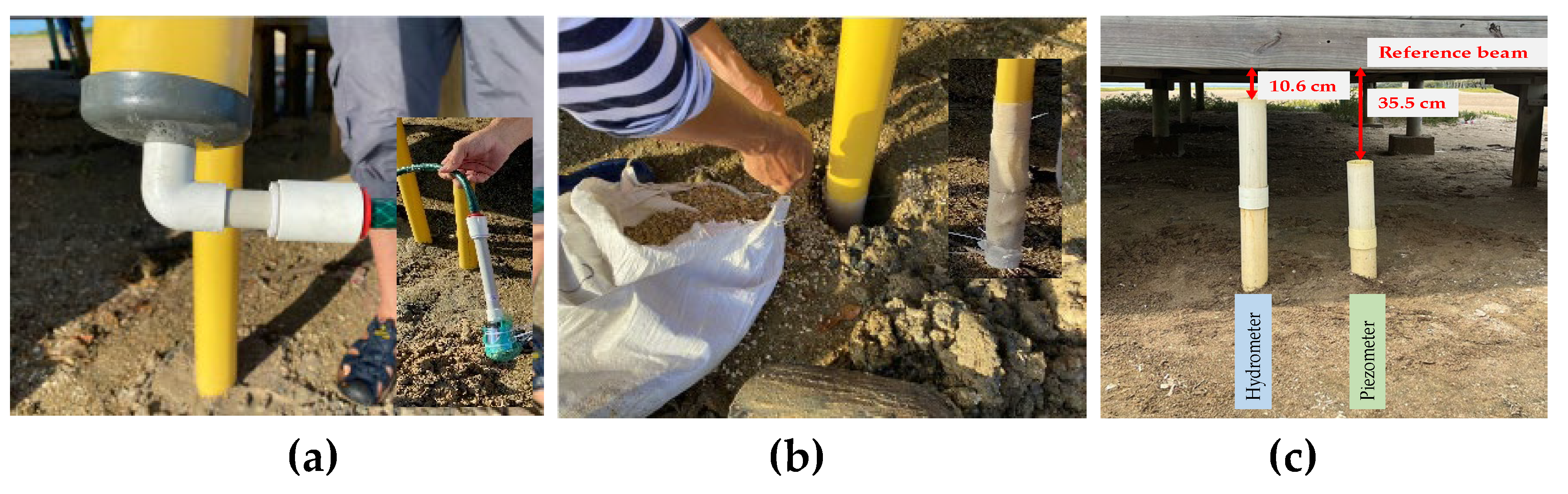
Figure 16.
Scheme of the construction details of the measuring systems: (a) hydrometer and piezometer.
Figure 16.
Scheme of the construction details of the measuring systems: (a) hydrometer and piezometer.
The reading, after training, was done by parks personnel twice a day, usually around 8 am and 4 pm. The operation consists in inserting a rigid rule inside the pipe with a block to set on the pipe edge and reading the wetted depth; from this, knowing the elevation of the reference beam edge, the elevation of water inside the pipe is determined. An alternative would have been a transparent cylinder with graduation marked on its external surface; however, the intense sunlight of the site would very soon deteriorate any plastic material, making reading impossible. The method adopted is more robust, but it requires to make a correction because, as shown in Figure 17, while inserting the rule (with a cross section a*b), there is a Δh super elevation that has to be removed from the reading.
This correction is determined by imposing that the volume increment inside the pipe be equal to the volume of the piece of rule wet, according to Equation 3a:
Δh*(Ac – a*b) = a*b *h (3a)
Ac = π D2/4: area of the pipe internal cross section
D [cm]: internal diameter of the pipe
h [cm]: depth of water inside the pipe already altered by the presence of the rule, that is partly wet (which is the reading effectuated by Parks staff)
Δh [cm]: height difference generated by the rule
a, b: dimensions of the rule stick (specifically: width, a= 3.8 cm; thickness b=1cm).
from which one obtains the correction to be applied to the reading as shown in Equation 3b:
Δh(h) = a*b*h/(Ac – a*b) (3b)
2.4. Lagoon: Horizontality Hypothesis
A doubt arose about the fact that the water surface of the lagoon may not be horizontal all the time (or never), mainly because of wind effect or of the hydraulic conditions governing the input -output of water flows, when the mouth is open or when the river is flooding.
To ascertain whether the horizontality hypothesis can be acceptable we adopted two criteria:
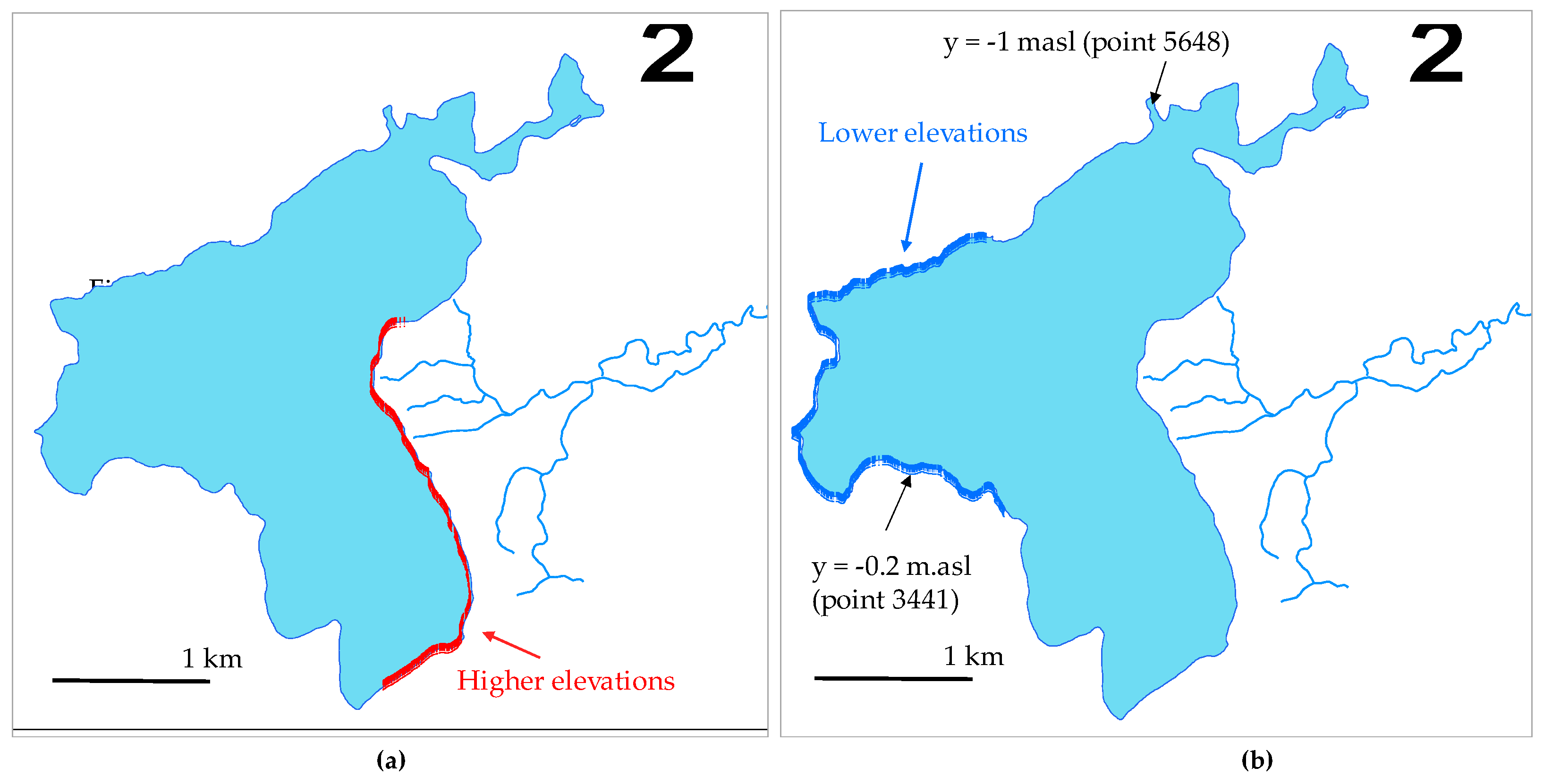
- “instantaneous altimetry”: The digital elevation model (DEM) we utilized is based on photogrammetry and was generated from an aerial image dataset collected in 2017 (generously provided by a national government agency called ‘Fondo de Adaptación). The resulting orthophoto mosaic survey can be assumed to be instantaneous and hence the elevation of the water surface border, all around the lagoon, would be constant be the hypothesis of horizontality verified. Unfortunately, the photo was taken in a dry period hence with a low level and hence small water surface so that structurally any difference cannot be very marked; nevertheless, from Figure 18 a certain nonuniformity is seemingly evident, indicating that there might have been indeed a certain degree of tilt;
- “synchronic monitoring”: by measuring with a relatively high frequency (every hour or so) the water elevation during a day both by our installed hydrometer and at the same time by an opposite point, namely the river at P. Viejo (so close to the lagoon that it can be assumed to coincide with its level in that point; see Figure 1), it should be possible to detect any height difference. The result shows a systematic elevation difference of approximately 15-20 cm between the two points (Figure 19).
The outcome of these tests is not that straightforward to interpret. The first test is consistent with the conclusion that a certain tilt does exist so that the horizontality hypothesis should be dropped. Possible reasons for this behavior are the sea outlet drawdown effect, the river input hydraulic load and winds seiches. However, the three campaigns were conducted in different days with different conditions of the mouth and only in November the river inflow was really significant, what eliminates the first two options, but would explain why the difference visible in Figure 19b is smaller, as the river carrying a higher flood rose a bit. In turn, frequent moderate winds are a reality, which would explain the presence of seiches.
However, as visible from Figure 20 and Figure 1, it would be logical that the object with higher elevation were the site at the river mouth (P.Viejo), but from Figure 19 evidently it is the reverse: the river elevation is always lower than the lagoon elevation at its hydrometer. Several explanations can be conceived. One, is that the seiche changes periodically and by chance all the three campaigns found an opposite situation than that of the satellite image of 2017. But this is very unlikely, including because our (qualitative) record of wind direction says that wind was more or less the same in the three conditions in terms of direction and intensity.
Another possibility is that the DEM assessment is not reliable; however, this hypothesis is likely to be dropped because we found a quite reasonable consistency between the elevations and surface areas derived from the DEM and the lagoon elevation measurements (see paragraph on morphometry). It may be possible, however, that it is reliable on the average, but the differences it shows (higher, lower zones) are not. A third possible explanation is that there is a structural bias in the topographic survey fixing the “zeros” of the hydrometers; this seems the most likely option as indeed although in both cases the survey started from official IGAC references, they were not physically coinciding owing to logistic constraints (absence of signal for the RTK equipment close to the lagoon mouth): an absolute difference between 20 and 40 cm is therefore possible. Resuming, we cannot conclude whether there is a tilt or not because according to the instantaneous test (DEM), there seems to be; but the time pattern test seems to contradict this conclusion as the detected difference is opposite in sign (what might however be explained by a different topographic reference) and, more important, in all the three days (with very different conditions of the mouth and of the river) kept the same sign and even the same absolute value (little less in the third case, but reasonably explained by the significant river inflow), what seems less likely and is more consistent with an hypothesis of identical level (i.e., horizontal surface or absence of tilt) plus constant topographic bias.
Figure 20.
Instantaneous altimetry test based on DEM analysis: Shore affected by lower (a) and higher (b) elevations; location of anomalous points: the most depressed one (y= -1 m.a.s.l) corresponds to the boca and most probably captured indeed the sea surface; the highest one, instead, lies in the nowhere and seems to be a local imperfection.
It is however important to observe that the measurement station of the lagoon level (hydrometer and piezometer) lies outside of the likely affected zones (Figure 20 and Figure 1) so that, assuming that the identified conditions (higher and lower zones) do not rotate around the lagoon, the water surface measurements can be considered representative of the real water surface elevation, that is extremely important for monitoring and modeling purposes. The possible bias between the river hydrometer and the lagoon hydrometer is not affecting data acquisition because river elevation (at the other bridge) is used just to feed the local stage-discharge relationship (and the relationship with the upstream station P.Troncal that is using the same identical reference). The possible tilt of the lagoon water surface could be affecting however the hydrodynamic modelling.
In any case, investigation still goes on to fully understand what is happening there. As a collateral note, it is important noting that the data on which this discussion is based cannot be considered exhaustive and fully representative as the DEM is quite imprecise (see par. 2.6), while our synchronic monitoring did not capture night time.
2.5. Lagoon: Exchange with the Sea
Being able to measure the exchange flow between the lagoon and the sea is key to set up a water balance; and even more when water quality is dealt with. The key issue then is finding a way to measure (or estimate) this flow in the simplest way.
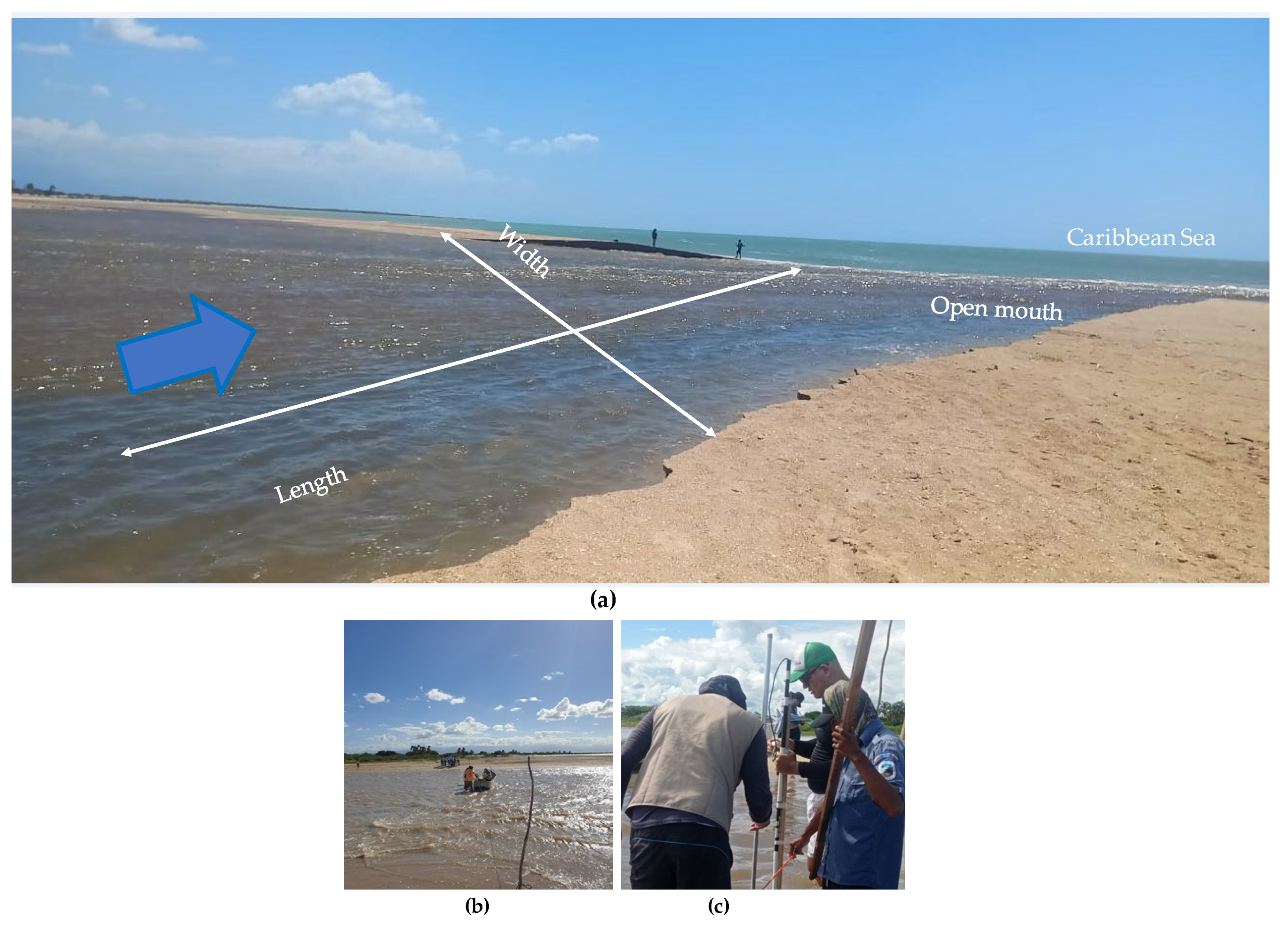
Normally, there is one or two periods of the year when the lagoon mouth (“la boca”) opens and a significant flow of freshwater outgoing occurs; after a few days, the flow alternates daily between outgoing and incoming depending on the tide (and possible additional river floods), until the mouth closes again. This is a quite complex phenomenon, not easy to measure and hard to predict. Indeed, the opening date depends mainly on the arrival of first significant river floods and this moment may vary greatly from year to year; and may occur twice a year, owing to the bimodal hydrological regime with two wet seasons from April to June and September to November, respectively [34]. Once the mouth is open, its geometry varies depending on the river inflow, the tide pattern and the average sea level, usually approaching a maximum area in about two weeks. That configuration is usually hold for one or two months and then the closure process starts, quite slow at the beginning and then accelerating, possibly during a month interval. The mouth area also varies during the day. But clearly this process is different every year. In 2022 the opening lasted 36 days (from May 29 until July 4); and the second opening period, usually stronger, lasted a bit more than 3 months (from the 21st of September 2022, until January 5 of 2023, lasting 106 days).
The key problem to be addressed at this stage of monitoring is however just measuring the water flow in several moments during the open mouth period, for both outgoing and incoming flows, and then set up a relationship that determines the exchange flow QB (positive or negative) as a function of, possibly, the height difference between the lagoon water elevation (yL) and that (yS) of the sea, that is (equation 4):
QB = QB(yL, yS) = QB(yL - yS) (4)
Probably, the most suited manner to carry out such a measurement is by a digital current-meter like ADCP (Acoustic Doppler, Current-meter Profiler) guided by a cable through the section. However, several reasons impeded this solution. Firstly, very pragmatically, our institution does not owe such a device and the regional environmental authority was reluctant to land us theirs because in brackish or salty water it can get soon spoiled. Secondly, the wind can get quite strong and so does the wave surge, and hence the device, floating on the surface, would move significantly and irregularly and the data would get very noisy. On the other side, consistently with the framework adopted, we chose to keep the technology very simple and low cost: we just pulled a rope as a reference across the section and on board of a boat driven by hand through poles (an engine would alter measurements and easily get into troubles because of the vertical oscillations and irregular bottom), we measured every 2 or 3 m -detected by colored knots on the rope- the depth with a rule and the velocity with a current meter (actually, two different devices to have a quality check on data: Manufacturer General Oceanics Environmental, Model 2030R Mechanical and manufacturer The Geography Specialists, Gepacks brand, model MFP126) at a depth about 60% of the total depth to be hopefully more representative of the vertical averaged longitudinal velocity (see Figure 21).
By adopting this method, several measurements have been carried out in different conditions, capturing both outgoing and incoming flows and this allowed us to set up a reliable relationship as expected and hoped (as will be described in a forthcoming paper). Therefore, actual systematic monitoring here reduces to components already considered: the lagoon and sea water elevations.
Figure 21.
Details of the mouth and velocity measurement: (a) lagoon during an “open period; (b) Our vehicle for surveying the cross section; (c) Manual measurement of depth and velocity.
Figure 21.
Details of the mouth and velocity measurement: (a) lagoon during an “open period; (b) Our vehicle for surveying the cross section; (c) Manual measurement of depth and velocity.
2.6. Lagoon: Morphometric Relationships
As a basis for monitoring the storage changes, it is key to count with the functional relationships: elevation-surface area and elevation-volume; these changes are indeed a key component for the water balance. The water surface greatly varies with its elevation; this makes imperative to merge a topographic representation of the zone with a bathymetric one.
We disposed of a set of aerial images taken during the dry season (March, 17th, 2017) by a photogrammetric tripulated flight from an elevation of 1100 m above sea level (size of pixel: 20 cm). By using a photogrammetric processing (via the Agisoft Metashape® software), we generated an orthophotomosaic of the whole scene and a dense points cloud describing the topography of the surrounding area around the lagoon. These points were manually edited and classified by using the tool ‘Auto-Classify ground points’ of Global Mapper ®.
The bathymetry in turn was reconstructed based on a set of 111 lagoon bottom elevation measurements directly determined by a GNSS-RTK from a boat, during 19, 20 of September 2022, together with a SIG supported spatial analysis. The spatial pattern of measurement points reflects more operational navigation constraints (wind, depth, distance) than a logical planning (Figure 22).
The adopted GIS strategy (ArcMap 10.8) to generate the bathymetric surface is articulated in 6 steps: i) Geo-statistical interpolation (Kriging) of acquired points via GNSS-RTK. ii) Extraction and smoothing of resulting elevation curves. iii) Interpolation of curves through TIN. iv) Rasterization of the TIN generated. v) Conversion of the bathymetric raster into a cloud points format“*.las” by utilizing the option “Export Layer to New File” in Global Mapper. vi) Integration and interpolation of the photogrammetric points cloud and bathymetric surface to achieve their connection and thus the final topo bathymetric DEM. For this last step, we adopted the tool “LAS Dataset to Raster” of ArcMap 10.8.
Independently, measurements of depth were taken by a sonar device (Garmin Striker) during the same bathymetric campaign, while in dry conditions we carried out point GNSS-RTK measurements in the floodable zone of the lagoon (then in dry conditions). All this was done to create a database with which validation of the generated topo-bathymetric DEM would be possible.
The key outputs of this activity are the surface area-elevation S(y) and volume-elevation V(y) relationships which have been obtained by points (Figure 23) by means of the r.lake.xy module, a spatial modeling tool hosted in GRASS GIS ® software. This module fills the water body (topo-bathymetric DEM) from a given elevation until a specified elevation is achieved. This tool requires in input a raster DEM, a maximum water elevation and its location coordinates (x,y).
A final, key check was to ascertain the coincidence of DEM elevation with measurements of the lagoon water surface. More precisely, the idea was to identify some dates with different conditions of the lagoon (at least 4); given the date, we would determine the area of water surface from satellite image (transformed into a polygon and eliminating possible “holes”) → then, from the inverse curve y = y(S), we would get the elevation y to be compared with the elevation measured that day at the hydrometer-piezometer devices and determine a fitting measure. We got a RMSE value of just 8,4 cm (Table 1) considered satisfactory (notice that, in addition to all uncertainties and approximations, there also is the exact hour of measurement that, as already said, occurred just twice a day, so both values were conserved).
2.7. Evaporation, Inflow from Runoff and Direct Precipitation
Evaporation from the lagoon water surface is obtained as surface area times the evaporation rate e(t) [mm/day]; as the former is already monitored, the simplest way is to acquire data about the relevant meteo-climatic variables already monitored in some nearby gauging station (visible in Figure 3) and then apply a suitable literature formula. Among the existing stations, the only one with data in our period is Camarones (point in Figure 3). It has to be noted however that –apart the rainy days- the meteorological conditions are quite constant in the area with strong solar radiation, temperature, low cloudiness, moderate to strong winds and so evaporation does not vary much (Figure 24) and consequently a constant value of 2 mm/day has been adopted.
To determine the direct precipitation input to the lagoon it is sufficient to know the precipitation itself, again one of the classic variables already measured in nearby stations. The only issue is ensuring their availability for the period of interest for ex-post simulations and its continuous measurements for the new monitoring. Luckily there exists a rainfall gauging station of the official IDEAM network (available at http://dhime.ideam.gov.co/atencionciudadano/Instituto) in the nearby town of Camarones (Figure 3).
For the runoff from the local catchment draining into the lagoon, basically the same discourse holds, although a kind of rainfall-runoff model has to be developed, which is described in another forthcoming paper.
3. Results and Discussion
Figure 25 shows the output of the monitoring exercise obtained until this paper has been written. The sea data shown are the original ones, without the correction established (see Par. 2.2) just to avoid overlapping of curves and allow an easier interpretation of the figure. It is apparent that the hourly tidal cycle is well hidden behind additional oscillations that are quite complex and irregular; moreover, there appears to be a growing trend (notice that a 500 steps interval corresponds to 20.8 days which is approximately a Moon month).
The data from the piezometer and the lagoon hydrometer are quite consistent in general, although with a certain deviation. Many factors can intervene like wind pressure that certainly acts more directly on the free water surface than on the underground phreatic surface, or reading errors. Apart the initial period (until April 4, 2022 when actually the devices where adjusted and deepened), it can be noted that for low levels, the piezometer provides higher values; while for high levels, in most of cases the opposite occurs. Consistently with the spirit of the two devices, we decided to utilize the hydrometer data for y (cm.a.s.l) > -20 (cm.a.s.l) which is where the feeding tube is certainly fully immersed, while the piezometer data are utilized below that threshold.
It is worth noting that, in spite of their numerosity, there are only two actual measures a day and this means that it is well possible that those data do not capture the maximum and minimum values (i.e., as already noted the sampling frequency is not high enough to capture the whole phenomenon). This is why they are represented as points with no connecting lines.
The behavior of the lagoon level is fully consistent with the status of the boca: as soon as it opens (fully or partly), the surface starts to oscillate synchronically to the sea tide. While, as soon as the boca closes, the level starts dropping because of evaporation, unless a flood input comes from the river. It is also apparent, however, that several river inputs are missing or underestimated Top graph), as unavoidable because the river has been measured just once a day.
A system quite similar to ours is described by Thompson et al. (2009) for some North African coastal lagoons. However, to measure the water level they adopted both human read hydrometers (or “stage boards”) and a set of automatic sensors (that could not be installed everywhere). Their effort, differently from ours, was not aiming at providing all the variables needed to set up a water balance; in particular, they did do not measure the lagoon-sea water exchange, although interesting observations are provided. In addition, they explore how the tidal effect propagates across the lagoon, but they do not show the simultaneous plot of the relevant variables that is illuminating when searching for a cause-effect relationship.
It must be emphasized that our system is based on a participatory basis, thanks to the very nice relationship established with National Parks institution, and staff as well. Particularly, a number of on-the-field training sessions and office seminars succeeded to motivate the personnel on the usefulness and reliability of the exercise they were involved in. This collaboration, started in an experimental fashion, is now passing to a more permanent status. Also, some local people have been directly involved in providing information and executing some measurements. We can state hence that the exercise has involved a significant participatory dimension. Anyway, honestly speaking, a systematic, long term monitoring certainly cannot be based on a voluntary effort only; the benefits of counting with such a system will be evident only in the long run and hence cannot be a sufficient solid reason to motivate local stakeholders to take in charge the operation of the system alone; only Parks can potentially hold the commitment on a long term horizon, but even this may not be guaranteed as each year some personnel adjustments take place. This is why a long term agreement between the local University and National Parks has been proposed and is being considered.
A completely different issue is that concerning sediment balance; in occasion of the river flow measurements, a water sample was taken to assess the suspended solids concentration SS with the hope to build a relationship with the flow, i.e., SS=f(Q) and analogous data for the sea in front of the lagoon mouth are available from other entities (although with a much lower frequency). But the difficulty is to measure the bed load flow carried by the river and through the lagoon mouth (in and out). We attempted several methods, but at the moment our hopes rely on a macro scale, i.e., observing the morphological evolution delta of Tomarrazón-Camarones River, which seems to be prograding into the lagoon. A direct comparison of satellite images and aerial photos can provide a first estimate; while the analysis of a DEM of differences of the same area might allow us to perform a quantitative estimation; but much longer times are required to cope with the vertical precision of drone images (at the moment we performed a first surveys by creating control points where vertical bars of known position and depth have been installed to observe, in the future, a possible aggradation of the floodplain). A key element, in addition, will be the coring of the sediment bed and its stratigraphic and dating analysis.
4. Conclusions
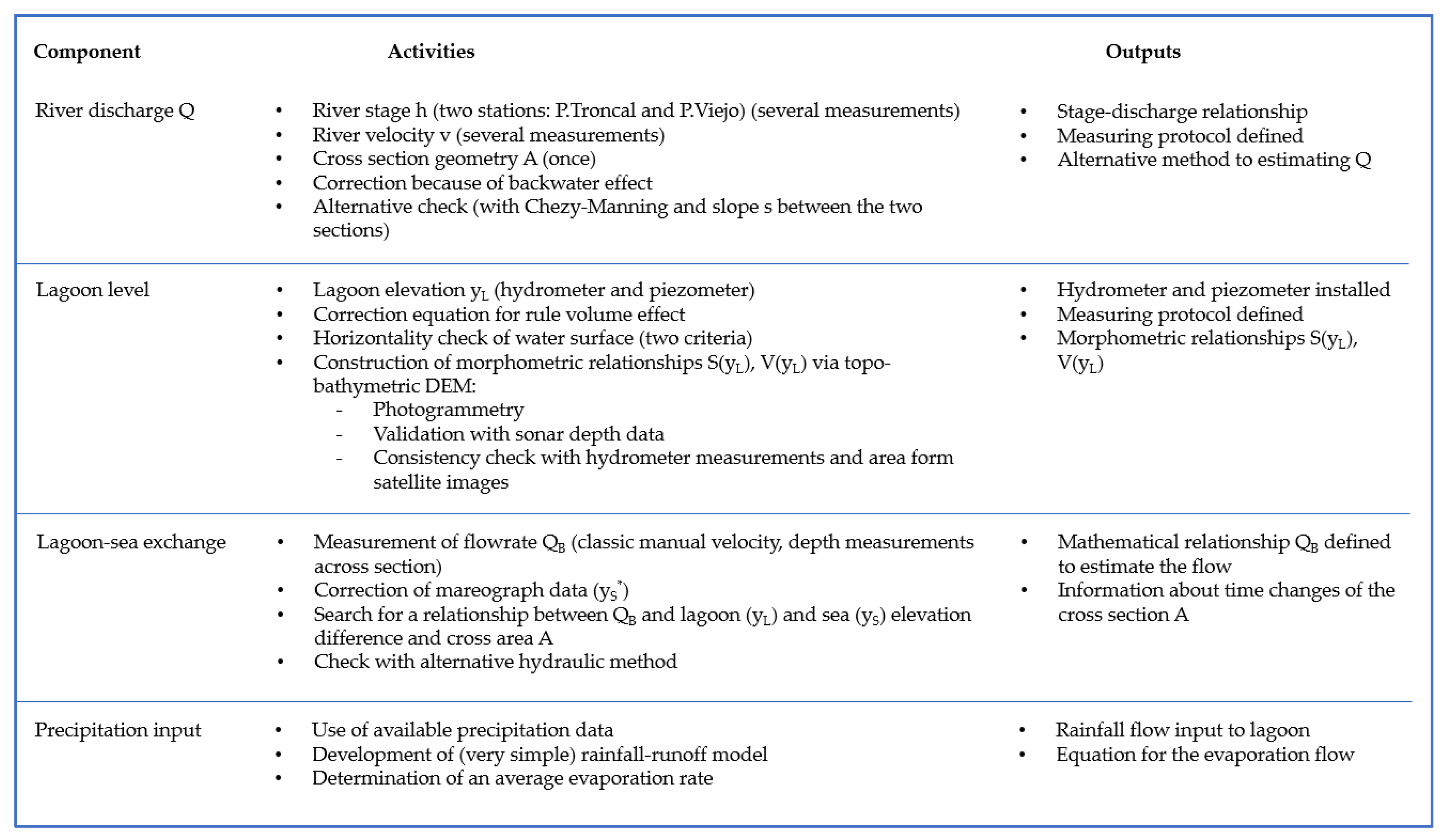
Conceiving and installing a monitoring system for the Camarones lagoon has been a small adventure through which many doubts have been solved and suitable methods and tools have been tested and applied; Figure 26 summarizes the key components of the whole exercise.
Figure 26.
Summary of the whole exercise conducted to set up the hydrological monitoring system.
The system is sufficiently reliable, as the various consistency tests (alternative estimation methods, matching graphs) and the observation of outputs demonstrate. Some weaknesses are nevertheless evident, as the frequent lack of river inputs data.
Although the project already provided information suitable to test a simulation model, which will be described in a forthcoming paper, it is intended to be continued and strengthened. A significant improvement would be the ability to monitor continuously (at least hourly) the river inputs; at the moment, the only way to address this need seems to be the installation of a basic automatic station, integrated by the manual monitoring already put in place and with the awareness that the devices will have to be replaced with a certain frequency because of damages and robbery. Certainly, an automatic station can also be installed in the lagoon site, much more protected, again in parallel with the manual monitoring.
The last point will be the analysis of the future under climate change, by setting up future scenarios of river inflow, evaporation rates and sea level rise, and hypothesizing the morphological evolution.
This experience may clash with the latest groovy advances of science, like in situ automatized sensors, remote sensing, machine learning and digital twins. But it recalls that before the last technological advances, science may emerge even through old, very simple methods when rooted in a sincere, humble search for insight.
Author Contributions
For research articles with several authors, a short paragraph specifying their individual contributions must be provided. The following statements should be used “Conceptualization, AGCN; methodology, AGCN, JIPM; software (to elaborate DEMs and specific Excel sheets to analyze and plot data), JREV, AGCN, JIPM; validation JIPMand AGCN; formal analysis, AGCN; investigation, JIPM, JREV; resources, JIPM, JREV; data curation, JIPM, JREV, AGCN; writing—original draft preparation, AGCN; writing—review and editing, JIPM, JREV; visualization, JIPM, AGCN, JREV; supervision, AGCN; project administration, JIPM; funding acquisition, JIPM. All authors have read and agreed to the published version of the manuscript.” Please turn to the CRediT taxonomy for the term explanation. Authorship must be limited to those who have contributed substantially to the work reported.
Funding
“This research was funded by Ministerio de Ciencia, Tecnología e Innovación of Colombia, call for proposals 890-2020, project 82511, resources administered by the Colombian Institute of Educational Credit and Technical Studies Abroad – ICETEX, but a self-funding share was necessary at the beginning as the start of the formal project suffered a significant delay or about three years.
Data Availability Statement
data generated within this effort are available under direct request to the corresponding authors.
Acknowledgments
This research is grateful to the Universidad de La Guajira for the contributions and grant to Professor JIPM; to the CREACUA Foundation (Riohacha, Colombia) for the impulse given to this initiative. A special greeting goes to Parques Nacionales Naturales de Colombia, and particularly to all the public servants of the Santuario de Fauna y Flora los Flamencos and their illuminated director Nianza Angulo Paredes. We also want to warmly thank Rosa Rodriguez Fernandez for the support in the installation of the measurement systems as well as Jose Fragozo Arevalo for the help in the topographic surveys. Last, but not least, a warm thank to Yesenia Zuñiga for her help in the preparation of figures.
Conflicts of Interest
The authors declare no conflicts of interest.
References
- Kennish, M.J.; Paerl, H.W. Coastal Lagoons : Critical Habitats of Environmental Change; ISBN 9781420088304.
- Pérez-Ruzafa, A.; Molina-Cuberos, G.J.; García-Oliva, M.; Umgiesser, G.; Marcos, C. Why Coastal Lagoons Are so Productive? Physical Bases of Fishing Productivity in Coastal Lagoons. Science of the Total Environment 2024, 922. [CrossRef]
- Pérez-Ruzafa, A.; Marcos, C. Fisheries in Coastal Lagoons: An Assumed but Poorly Researched Aspect of the Ecology and Functioning of Coastal Lagoons. Estuar Coast Shelf Sci 2012, 110, 15–31. [CrossRef]
- Velasco, A.M.; Pérez-Ruzafa, A.; Martínez-Paz, J.M.; Marcos, C. Ecosystem Services and Main Environmental Risks in a Coastal Lagoon (Mar Menor, Murcia, SE Spain): The Public Perception. J Nat Conserv 2018, 43, 180–189. [CrossRef]
- Thompson, J.R.; Flower, R.J.; Ramdani, M.; Ayache, F.; Ahmed, M.H.; Rasmussen, E.K.; Petersen, O.S. Hydrological Characteristics of Three North African Coastal Lagoons: Insights from the MELMARINA Project. Hydrobiologia 2009, 622, 45–84. [CrossRef]
- Bedoya Vásquez, C.J. Caracterización de La Pesquería Artesanal En La Laguna de Navío Quebrado, Departamento de La Guajira, Caribe Colombiano. Trabajo de grado , Universidad Jorge Tadeo Lozano: Bogotá, 2004.
- 2008; 7. Corporación Autónoma Regional de La Guajira [CORPOGUAJIRA] Plan de Ordenamiento y Manejo de La Cuenca Del Río Tomarrazón-Camarones; Riohacha, 2008.
- Urrego, L.E.; Correa-Metrio, A.; González, C.; Castaño, A.R.; Yokoyama, Y. Contrasting Responses of Two Caribbean Mangroves to Sea-Level Rise in the Guajira Peninsula (Colombian Caribbean). Palaeogeogr Palaeoclimatol Palaeoecol 2013, 370, 92–102. [CrossRef]
- Parques Nacionales Naturales de Colombia Programa de Conservación Del Flamenco En El Santuario de Fauna y Flora Los Flamencos, Departamento de La Guajira, Costa Caribe de Colombia; Ediprint Ltd.a, Ed.; Bogotá, Colombia, 2013; ISBN 978-958-8426-42-6.
- Rosado Vega, J.R.; Castro Echavez, F.L.; Márquez Gulloso, E.R. Environmental, Biological, and Fishing Factors Influencing Fish Mortality and Development of the Cachirra Event, Navío Quebrao Lagoon. Tecnura 2022, 26, 17–41. [CrossRef]
- Cardona, L. Non-Competitive Coexistence between Mediterranean Grey Mullet: Evidence from Seasonal Changes in Food Availability, Niche Breadth and Trophic Overlap. J Fish Biol 2001, 59, 729–744. [CrossRef]
- Moreno-M, G.P.; Acuña-Vargas, J.C. Caracterización de Lepidópteros Diurnos En Dos Sectores Del Santuario de Flora y Fauna Los Flamencos (San Lorenzo de Camarones, La Guajira). Boletin Cientifico del Centro de Museos 2015, 19, 221–234. [CrossRef]
- 2022; 13. Corporación Autónoma Regional de La Guajira [CORPOGUAJIRA] Ajuste y/o Actualización Del POMCA Del Río Camarones y Otros Directos al Caribe – La Guajira; Riohacha, Colombia, 2022;
- 2017; 14. INVEMAR Concepto Técnico Sobre La Mortandad de Peces Ocurrida En La Laguna Navío Quebrado (Corregimiento de Camarones, Municipio de Riohacha En La Guajira) En Agosto de 2017, CPT-CAM 021-17; Santa Marta, 2017;
- Blaen, P.J.; Khamis, K.; Lloyd, C.E.M.; Bradley, C.; Hannah, D.; Krause, S. Real-Time Monitoring of Nutrients and Dissolved Organic Matter in Rivers: Capturing Event Dynamics, Technological Opportunities and Future Directions. Science of the Total Environment 2016, 569–570, 647–660. [CrossRef]
- Chan, K.; Schillereff, D.N.; Baas, A.C.W.; Chadwick, M.A.; Main, B.; Mulligan, M.; O’Shea, F.T.; Pearce, R.; Smith, T.E.L.; van Soesbergen, A.; et al. Low-Cost Electronic Sensors for Environmental Research: Pitfalls and Opportunities. Prog Phys Geogr 2021, 45, 305–338. [CrossRef]
- Hamel, P.; Ding, N.; Cherqui, F.; Zhu, Q.; Walcker, N.; Bertrand-Krajewski, J.L.; Champrasert, P.; Fletcher, T.D.; McCarthy, D.T.; Navratil, O.; et al. Low-Cost Monitoring Systems for Urban Water Management: Lessons from the Field. Water Res X 2024, 22. [CrossRef]
- Kabi, J.N.; wa Maina, C.; Mharakurwa, E.T.; Mathenge, S.W. Low Cost, LoRa Based River Water Level Data Acquisition System. HardwareX 2023, 14. [CrossRef]
- Notter, B.; MacMillan, L.; Viviroli, D.; Weingartner, R.; Liniger, H.P. Impacts of Environmental Change on Water Resources in the Mt. Kenya Region. J Hydrol (Amst) 2007, 343, 266–278. [CrossRef]
- Frappart, F.; Blarel, F.; Fayad, I.; Bergé-Nguyen, M.; Crétaux, J.F.; Shu, S.; Schregenberger, J.; Baghdadi, N. Evaluation of the Performances of Radar and Lidar Altimetry Missions for Water Level Retrievals in Mountainous Environment: The Case of the Swiss Lakes. Remote Sens (Basel) 2021, 13. [CrossRef]
- Huang, Q.; Long, D.; Du, M.; Zeng, C.; Li, X.; Hou, A.; Hong, Y. An Improved Approach to Monitoring Brahmaputra River Water Levels Using Retracked Altimetry Data. Remote Sens Environ 2018, 211, 112–128. [CrossRef]
- Tourian, M.J.; Tarpanelli, A.; Elmi, O.; Qin, T.; Brocca, L.; Moramarco, T.; Sneeuw, N. Spatiotemporal Densification of River Water Level Time Series by Multimission Satellite Altimetry. Water Resour Res 2016, 52, 1140–1159. [CrossRef]
- Biancamaria, S.; Lettenmaier, D.P.; Pavelsky, T.M. The SWOT Mission and Its Capabilities for Land Hydrology. Surv Geophys 2016, 37, 307–337. [CrossRef]
- Wu, J.; Li, W.; Du, H.; Wan, Y.; Yang, S.; Xiao, Y. Estimating River Bathymetry from Multisource Remote Sensing Data. J Hydrol (Amst) 2023, 620. [CrossRef]
- Chow, V.T. Open-Channel Hydraulic; McGraw-Hill, Ed.; New York, 1959; ISBN 978-0-07-085906-7.
- Ferro, V. Comments on “Measurement of Dimensionless Chezy Coefficient in Step-Pool Reach (Case Study of Dizin River in Iran)” by Torabizadeh A., Tahershamsi A., Tabatabai M.R.M. Flow Measurement and Instrumentation 2018, 64, 190–193. [CrossRef]
- Tymiński, T.; Kałuża, T.; Hämmerling, M. Verification of Methods for Determining Flow Resistance Coefficients for Floodplains with Flexible Vegetation. Sustainability (Switzerland) 2022, 14. [CrossRef]
- Okhravi, S.; Schügerl, R.; Velísková, Y. Flow Resistance in Lowland Rivers Impacted by Distributed Aquatic Vegetation. Water Resources Management 2022, 36, 2257–2273. [CrossRef]
- Boutron, O.; Paugam, C.; Luna-Laurent, E.; Chauvelon, P.; Sous, D.; Rey, V.; Meulé, S.; Chérain, Y.; Cheiron, A.; Migne, E. Hydro-Saline Dynamics of a Shallow Mediterranean Coastal Lagoon: Complementary Information from Short and Long Term Monitoring. J Mar Sci Eng 2021, 9. [CrossRef]
- García, J., & Cuervo, E. Pronóstico de Pleamares y Bajamares En La Costa Occidental de Colombia Para El Año de 1978.; Instituto Geográfico Agustín Codazzi (IGAC), Ed.; Bogotá, Colombia, 1978;
- Álvarez Machuca, M.C.; Pulido Nossa, D.A.; Solano Trullo, L.J.; Oviedo Barrero, F. Construcción de La Superficie Hidrográfica de Referencia Vertical Para Las Bahías de Buenaventura y Málaga, Pacífico Colombiano. Boletín Científico CIOH 2018, 53–69. [CrossRef]
- Escobar Villanueva, J.; Nardini, A.; Iglesias Martínez, L. Evaluación Del Uso de Topografía LiDAR En El Modelado de Inundaciones Urbanas Con MODCEL ©. Aplicación a La Ciudad Costera de Riohacha, La Guajira (Caribe Colombiano).; Sevilla, October 21 2015; pp. 383–386.
- Shannon, C.E. Communication in the Presence of Noise. Proceedings of the IRE 1949, 37, 10–21. [CrossRef]
- Arregocés, H.A.; Rojano, R.; Pérez, J. Validation of the CHIRPS Dataset in a Coastal Region with Extensive Plains and Complex Topography. Case Studies in Chemical and Environmental Engineering 2023, 8. [CrossRef]
Figure 1.
Scheme of the typical hydrological-ecological cycle of a coastal lagoon in La Guajira: (a) dry season; b) flood season with opening of la boca and outflow of semi fresh water; (c) sea-lagoon exchange according to tide.
Figure 1.
Scheme of the typical hydrological-ecological cycle of a coastal lagoon in La Guajira: (a) dry season; b) flood season with opening of la boca and outflow of semi fresh water; (c) sea-lagoon exchange according to tide.
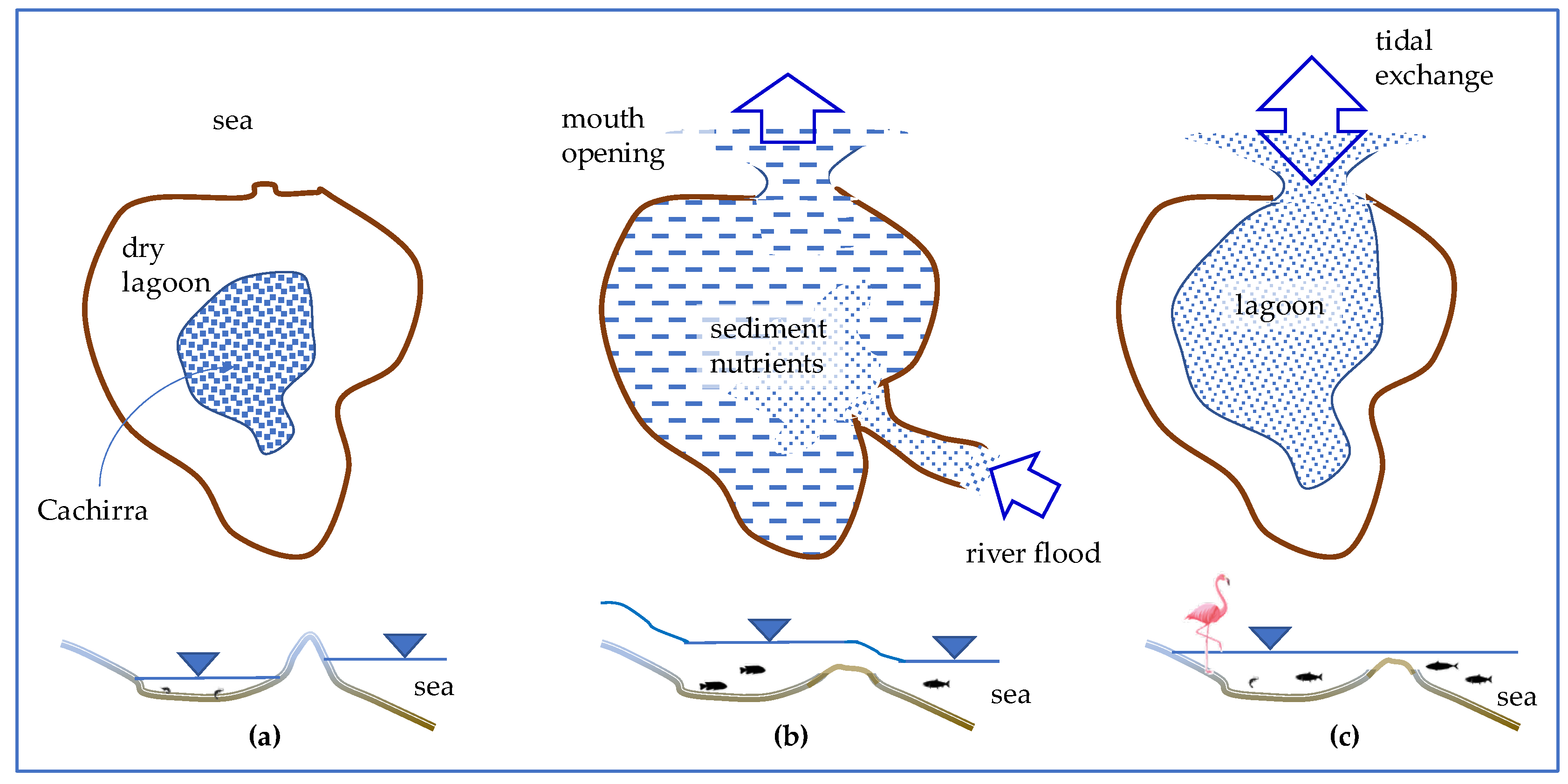
Figure 2.
Navío-Quebrado (Camarones) lagoon: (a) wet season; (b) opening of mouth (“la boca”); (c) the bar between sea and lagoon (closed mouth).
Figure 2.
Navío-Quebrado (Camarones) lagoon: (a) wet season; (b) opening of mouth (“la boca”); (c) the bar between sea and lagoon (closed mouth).
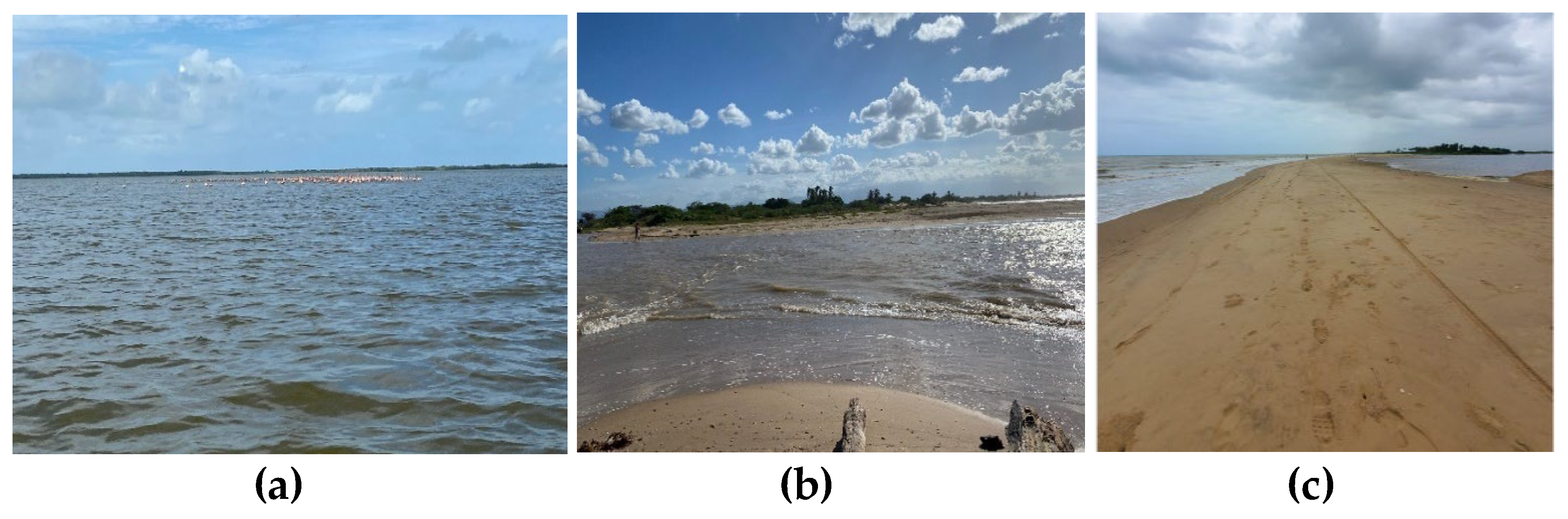
Figure 3.
Study area a) general location; b) location of specific interest points.
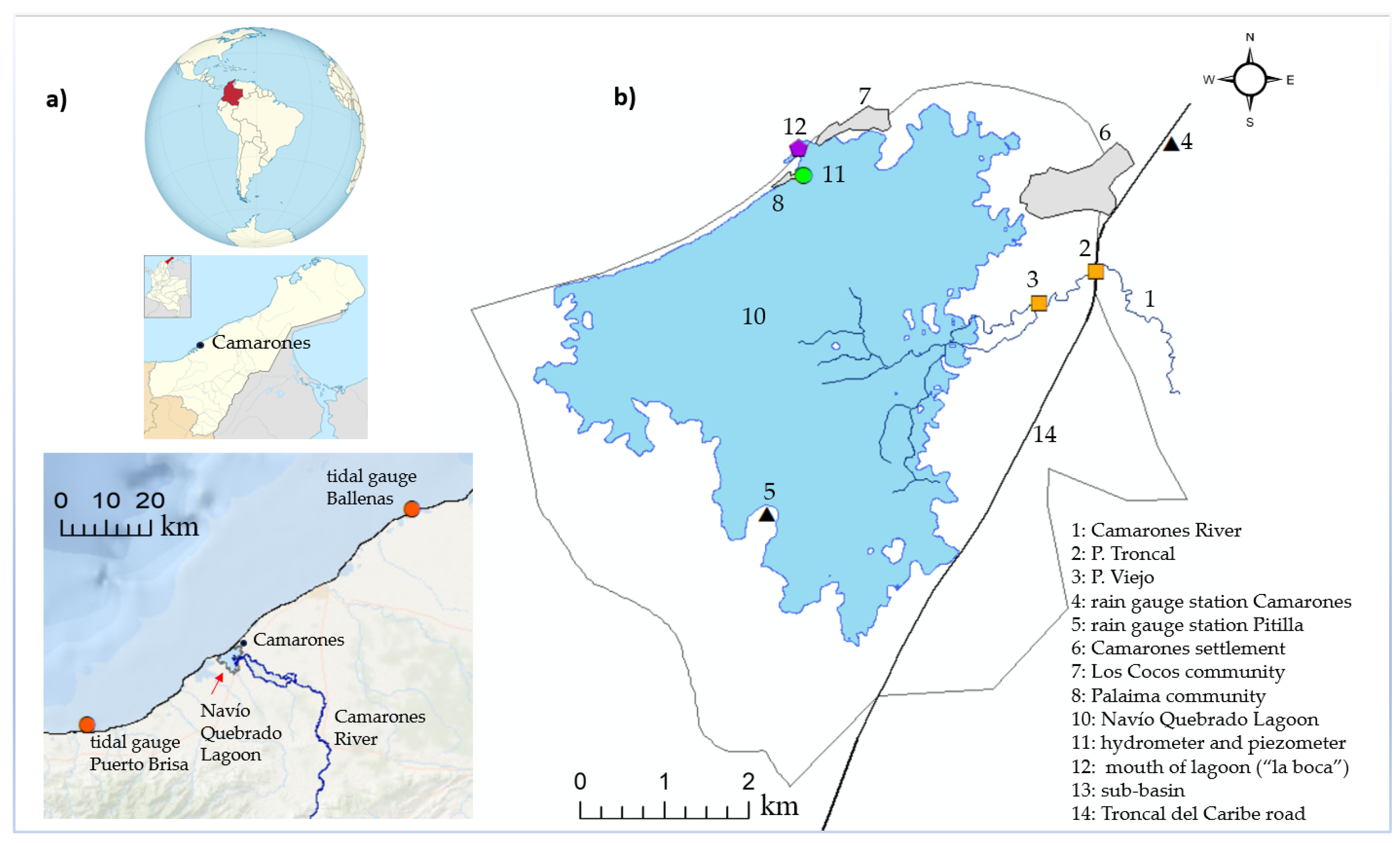
Figure 4.
Location of hydrometers: (a) view from downstream at Puente Troncal; (b) view from observation point at Puente Viejo; (c) rule at Puente Troncal; (d) rule at the same site during a flood (actually this is located on the opposite side of the pillar).
Figure 4.
Location of hydrometers: (a) view from downstream at Puente Troncal; (b) view from observation point at Puente Viejo; (c) rule at Puente Troncal; (d) rule at the same site during a flood (actually this is located on the opposite side of the pillar).
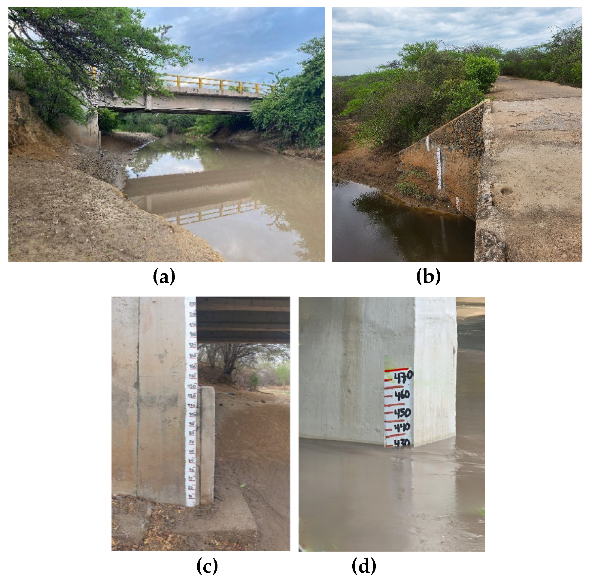
Figure 5.
Cross section at Puente Troncal. It can be noted that the 0 of the hydrometer was placed where water was at the day of installation; but the river can go lower (the depth was estimated by directly wading the section). This means, that negative values of the water height h are also possible.
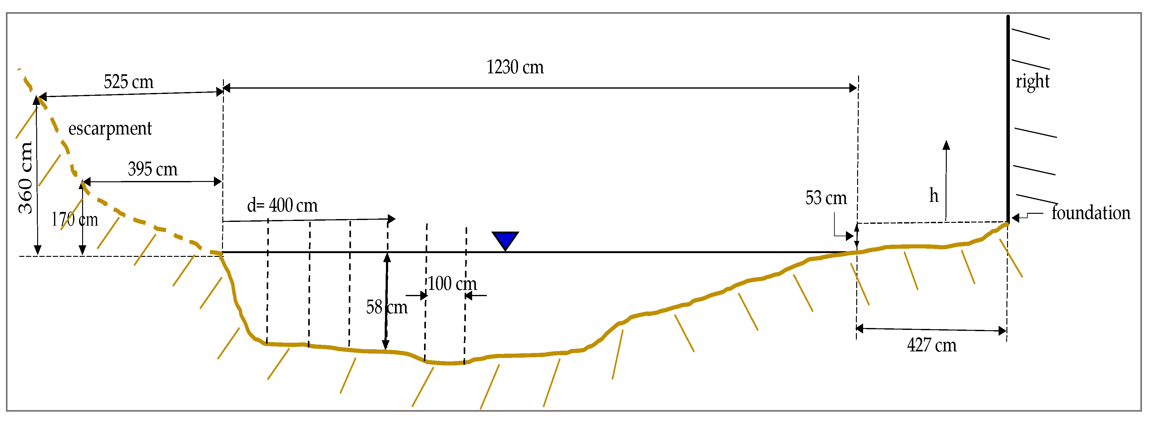
Figure 6.
Difficult Access to the measurements sites: (a) Puente Troncal; (b) Puente Viejo.
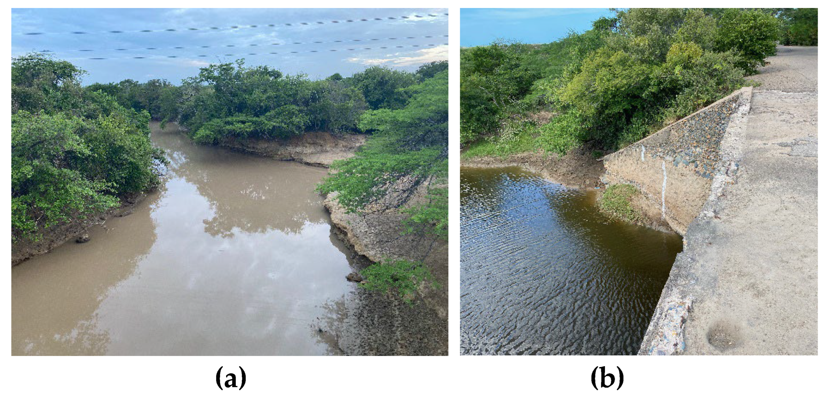
Figure 7.
Stage-discharge relationship (polynomial regression) of Tomarrazon-Camarones River in Puente Troncal with gauging data from 23 April 2022 until 23 October 2023 (y denotes elevation m asl).
Figure 7.
Stage-discharge relationship (polynomial regression) of Tomarrazon-Camarones River in Puente Troncal with gauging data from 23 April 2022 until 23 October 2023 (y denotes elevation m asl).
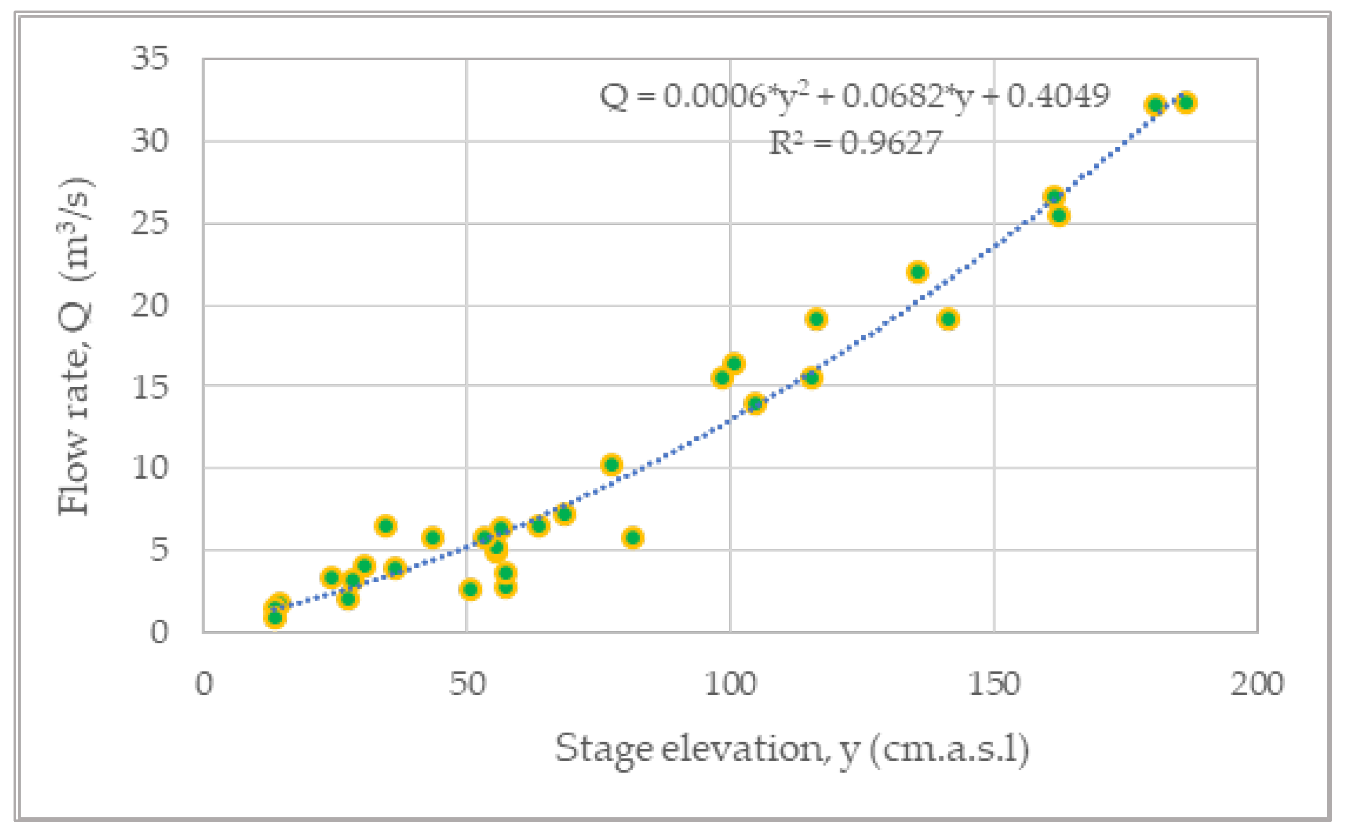
Figure 10.
Surprise from new data of Tomarrazon-Camarones River in Puente Troncal: (a) Stage-discharge relationship (power law regression, R2=0,9172) with gauging data from 23 Abril 2022 until 23 November 2023; (b) matching between measured and estimated values (red line: perfect matching, dotted line: linear regression with R2=0,9119).
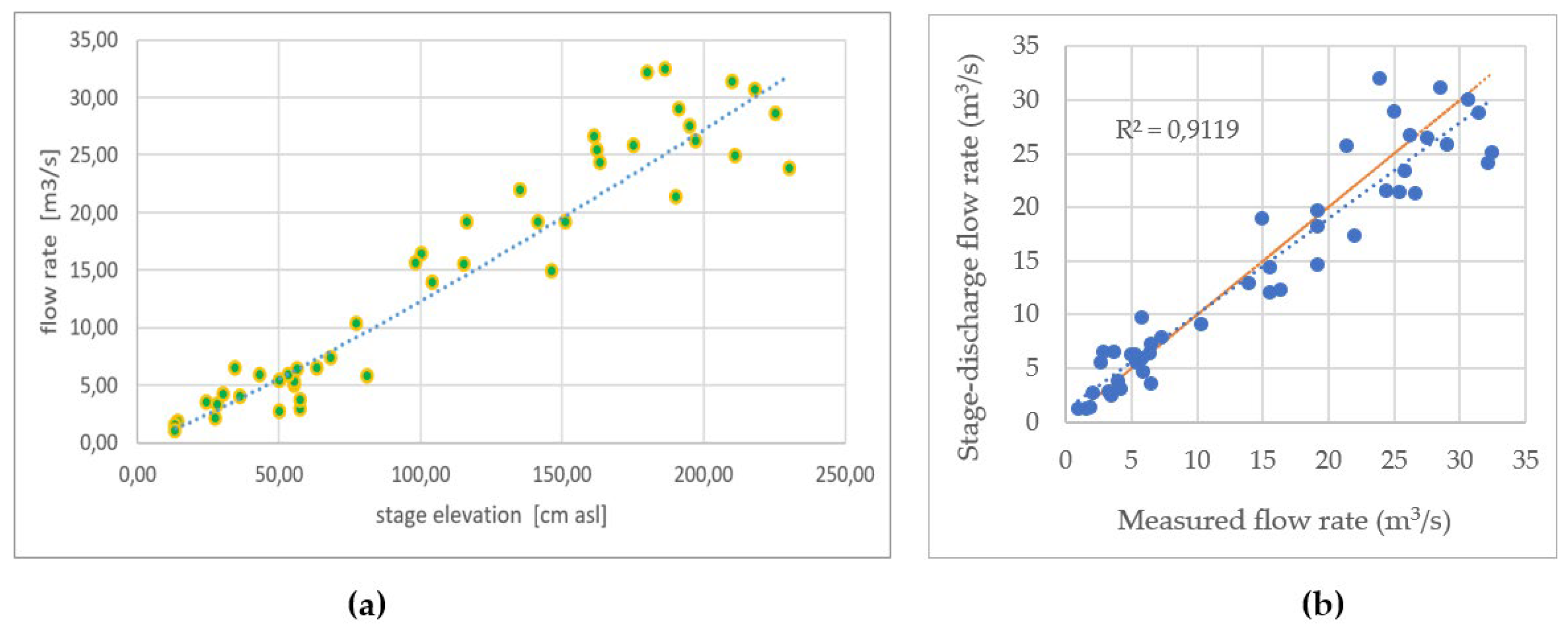
Figure 11.
Deviation Q measured vs Q estimated by the found stage-discharge relationship (m3/s) as a function of the water elevation yLagoon (in cm above sea level).
Figure 11.
Deviation Q measured vs Q estimated by the found stage-discharge relationship (m3/s) as a function of the water elevation yLagoon (in cm above sea level).
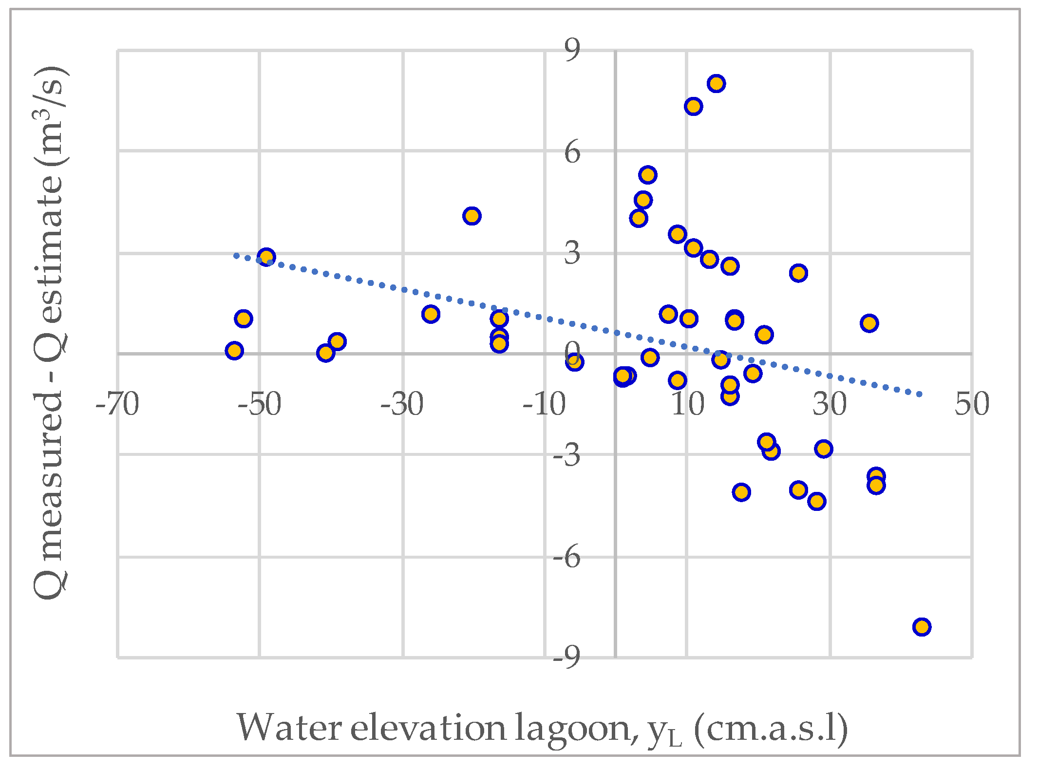
Figure 13.
Extract of the time series of recorded data (at hourly time step) showing the inconsistency between lagoon data and sea data, always higher than 0 and higher than the lagoon level (top: sea elevation data kindly provided by DIMAR: daily moving average in darker line; bottom: lagoon water elevation data collected by our project).
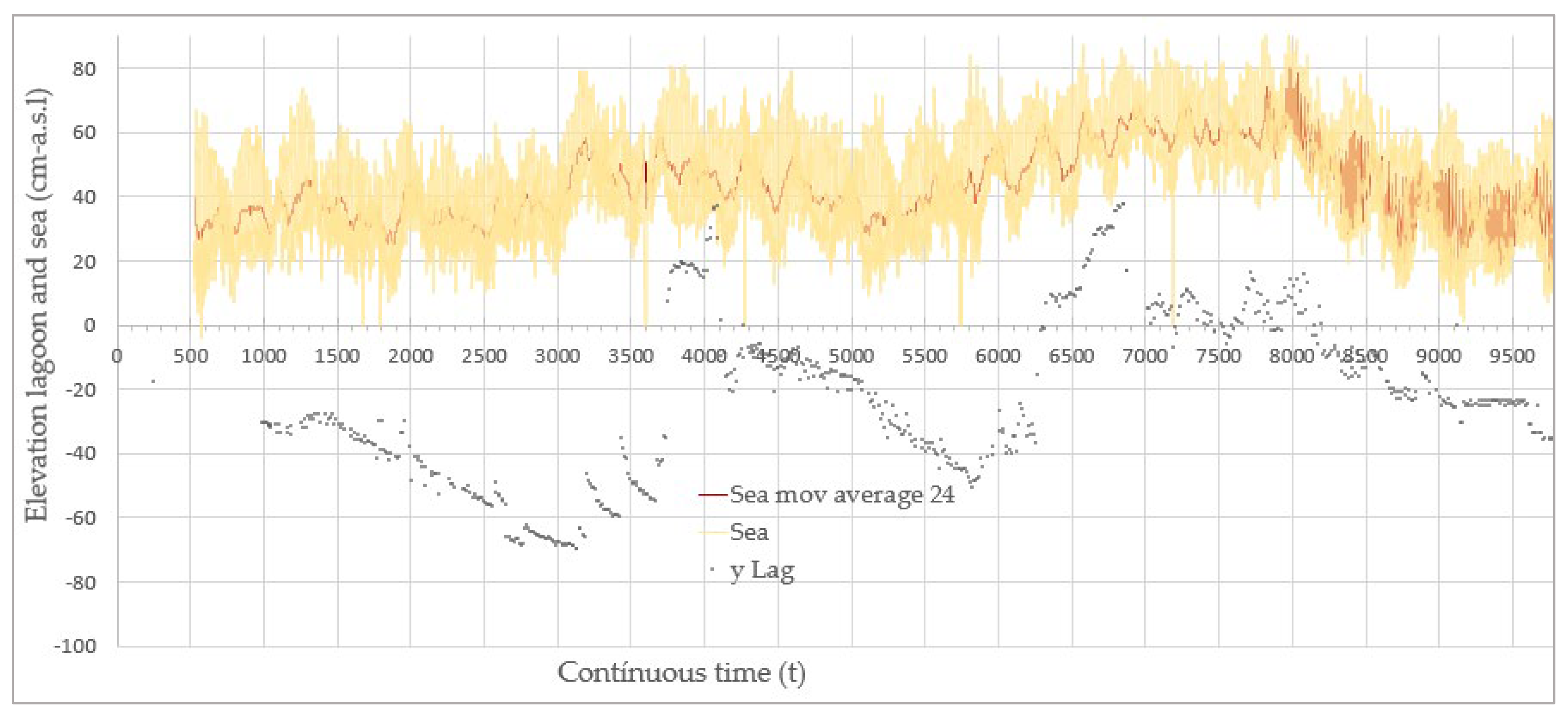
Figure 14.
General view of the lagoon water level measurement system.
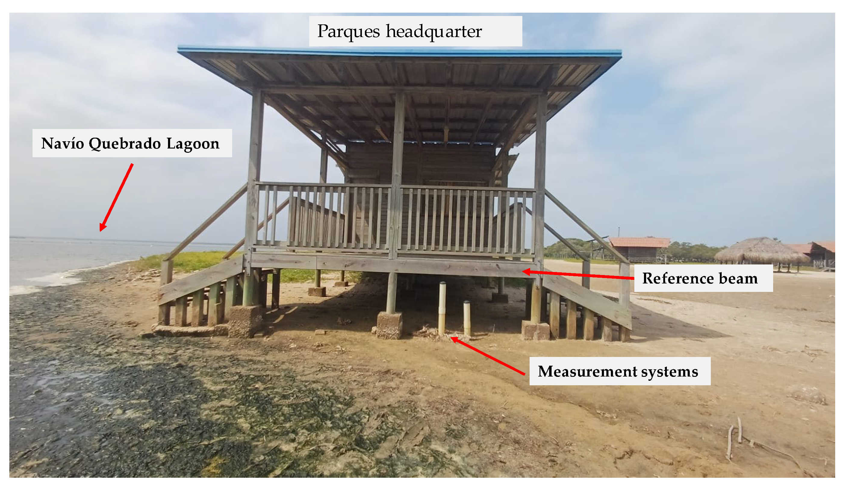
Figure 17.
Alteration of the measurement of the water level h because of the volume of the inserted rule.
Figure 17.
Alteration of the measurement of the water level h because of the volume of the inserted rule.
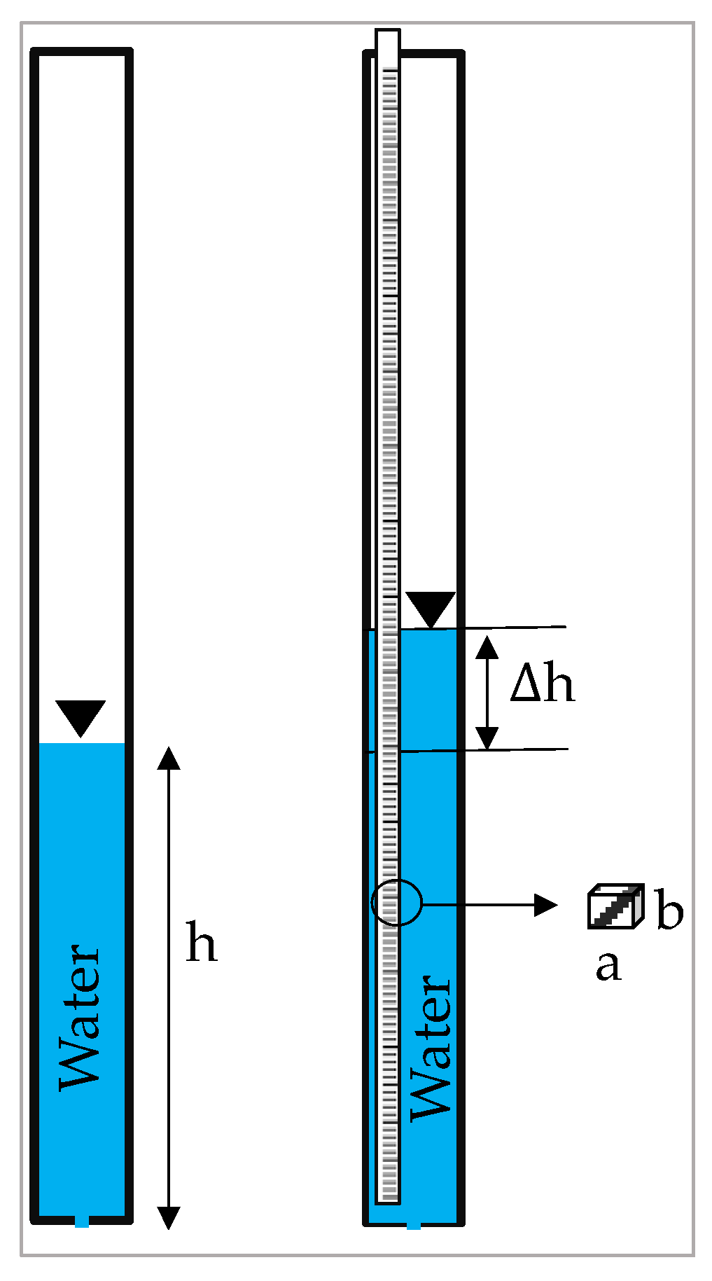
Figure 18.
Elevation pattern of lagoon perimeter according to satellite imagen 2017 (basis of the DEM adopted). The local peaks are attributed to DEM imperfections. The mean elevation is denoted by the brown bar.
Figure 18.
Elevation pattern of lagoon perimeter according to satellite imagen 2017 (basis of the DEM adopted). The local peaks are attributed to DEM imperfections. The mean elevation is denoted by the brown bar.
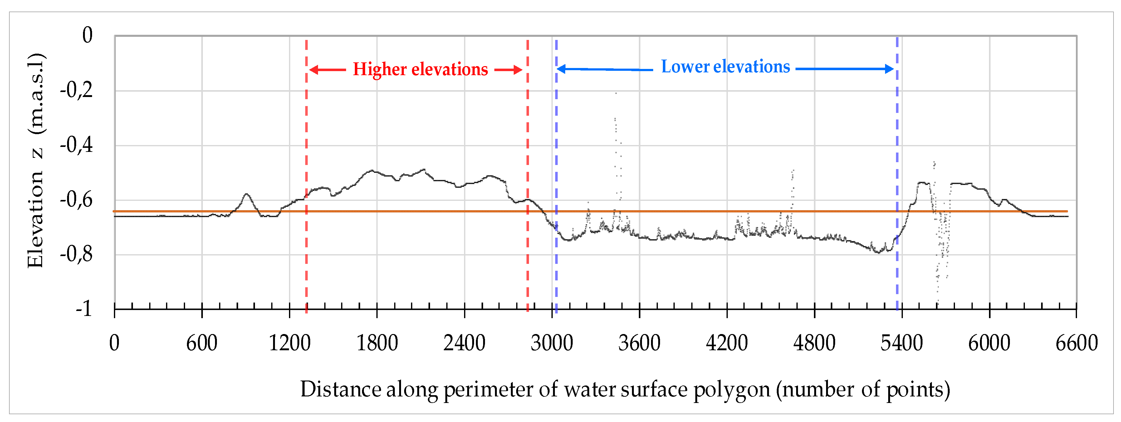
Figure 19.
Horizontality check: synchronic monitoring criterion: (a) original data obtained; (b) three sets of curves refer to three different days of survey (in May, no exchange with the sea nor river inflow and negligible evaporation effect during daytime, so constant values; in June, outgoing flow is emptying the lagoon, although a moderate river inflow was present; in November a significant river inflow is filling the lagoon, in spite of a moderate open mouth); the top curves refer to the lagoon, the bottom ones to the river at the same time: a synchronic behavior is apparent, as well as the existence of an elevation difference of about 12-20 cm.
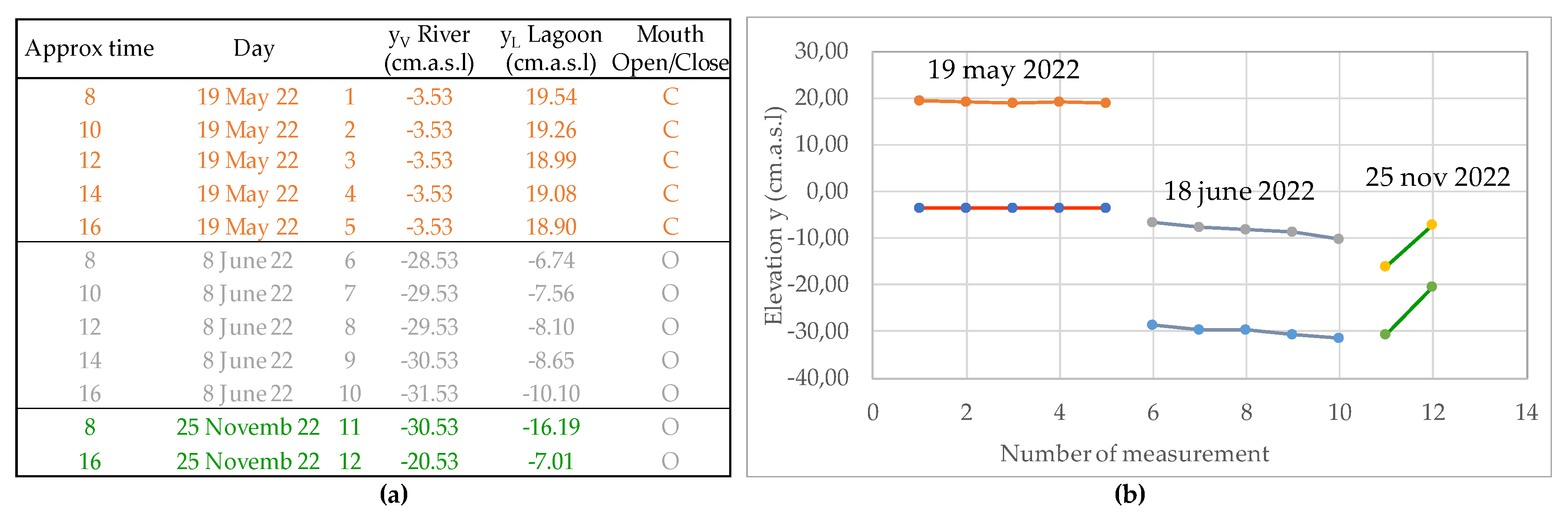
Figure 22.
Spatial pattern of 111 GNSS-RTK points (red). The background image is a Landsat 8 of 20 September 2022 when the lagoon was at maximum filling. The false color image identifies wáter (dark blue tone) under a combination of bands NIR, SWIR1 and Red.
Figure 22.
Spatial pattern of 111 GNSS-RTK points (red). The background image is a Landsat 8 of 20 September 2022 when the lagoon was at maximum filling. The false color image identifies wáter (dark blue tone) under a combination of bands NIR, SWIR1 and Red.
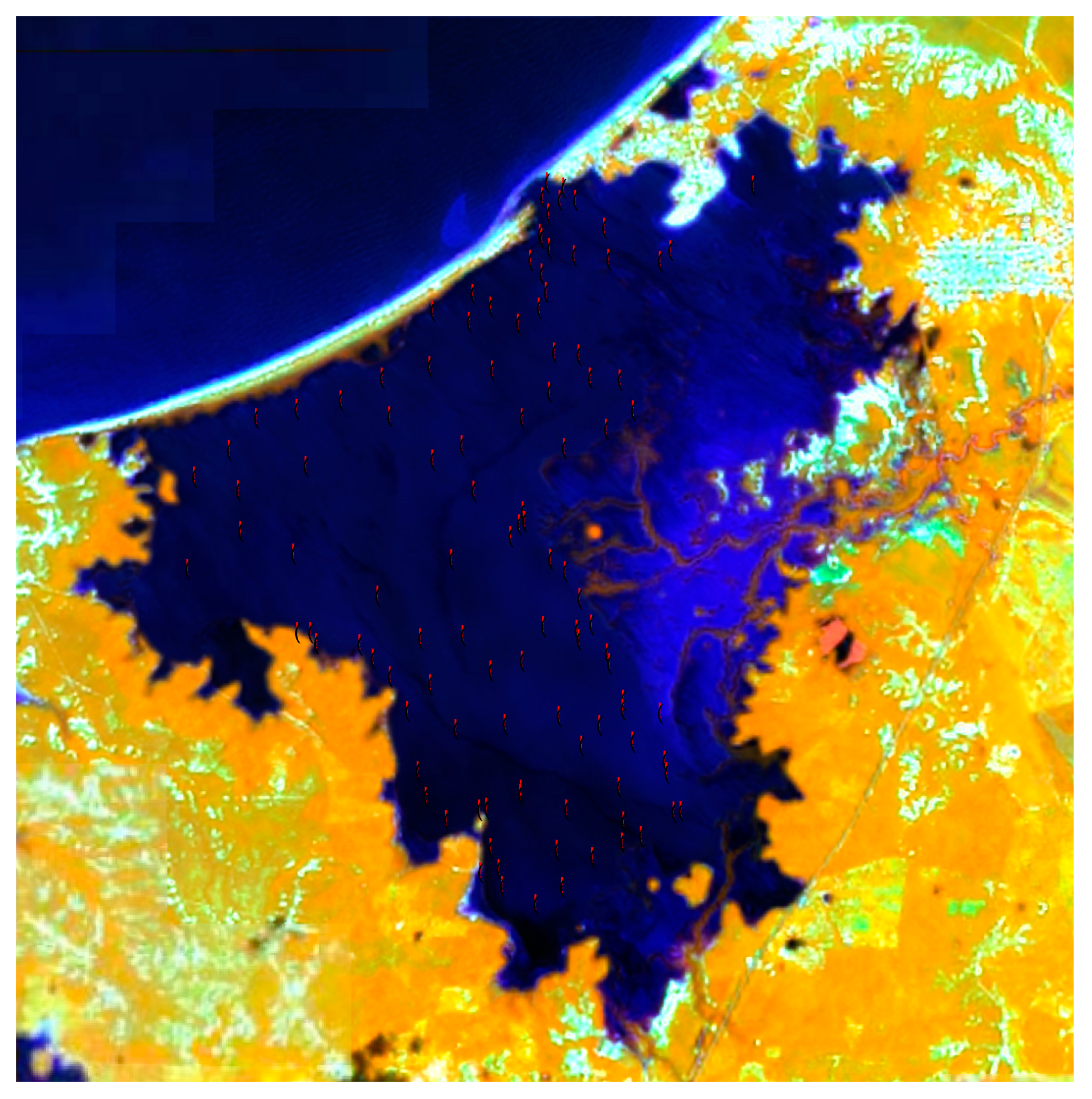
Figure 23.
Hypsometric curves: Surface area S = S(y) (m2); Storage volume V= V(y) (m3) related to lagoon elevation yL [masl]. Polynomial curves: S(y) = 8010914.35 y3 - 8335673.88 y2 + 7166288.16 y + 16056191.36 (R² = 1.00); V(y) = 4983114.71 y2 + 15272088.13 y + 8414661.47 (R² = 1.00).
Figure 23.
Hypsometric curves: Surface area S = S(y) (m2); Storage volume V= V(y) (m3) related to lagoon elevation yL [masl]. Polynomial curves: S(y) = 8010914.35 y3 - 8335673.88 y2 + 7166288.16 y + 16056191.36 (R² = 1.00); V(y) = 4983114.71 y2 + 15272088.13 y + 8414661.47 (R² = 1.00).
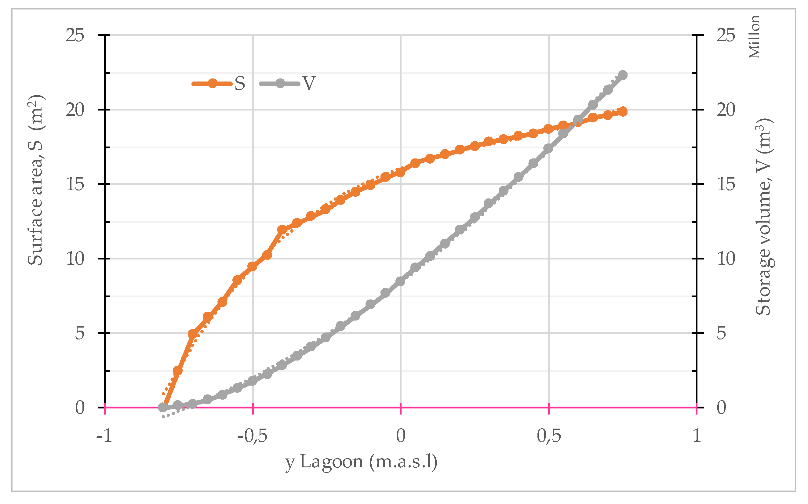
Figure 24.
Climatological variables of the study area (from IDEAM data: Rain from Camarones station ID 15050010. All others from Riohacha station ID 15065180.
Figure 24.
Climatological variables of the study area (from IDEAM data: Rain from Camarones station ID 15050010. All others from Riohacha station ID 15065180.
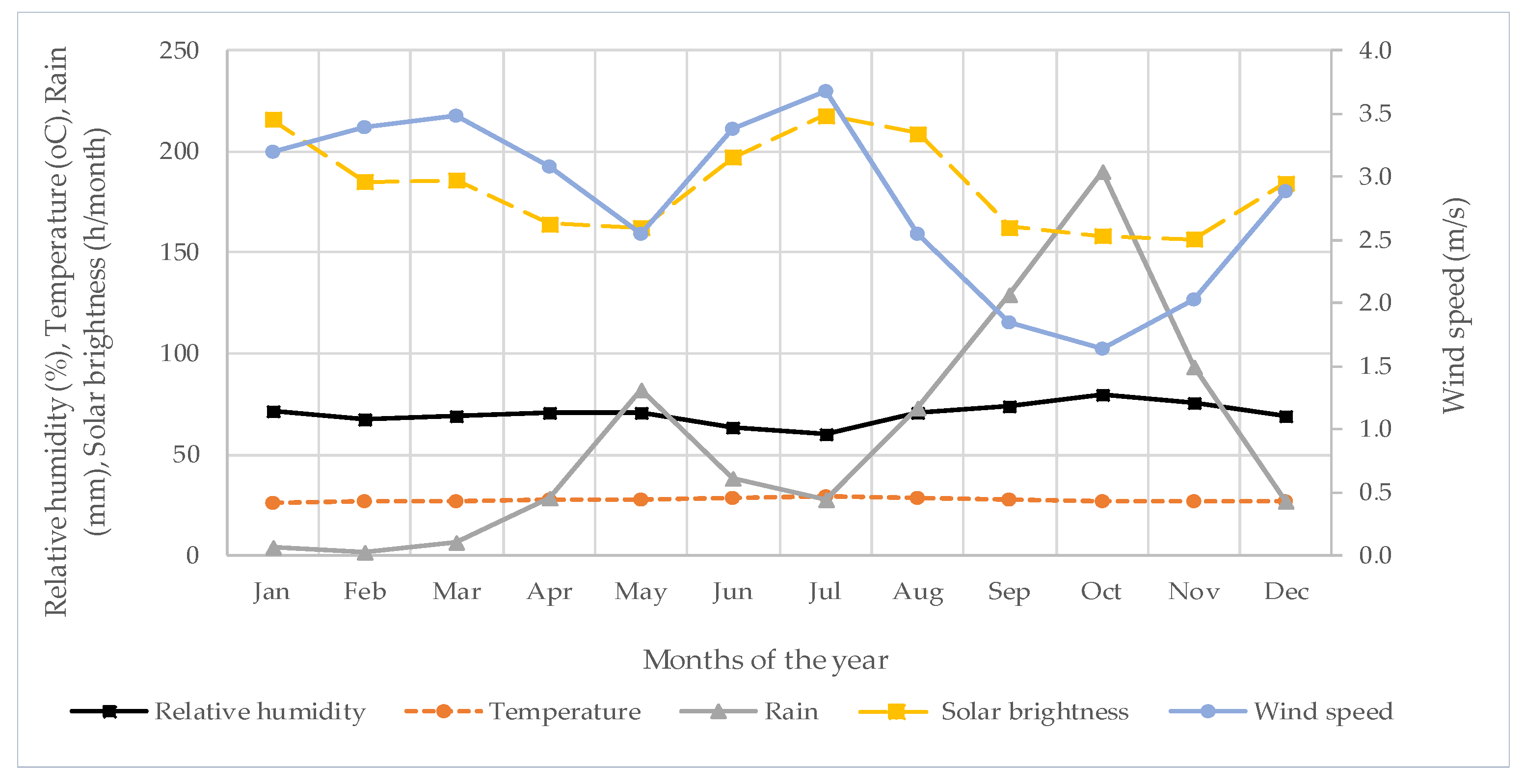
Figure 25.
Output of the monitoring system for the period December 10, 2021 to January 14, 2023 (hourly time step; una square is 500 hours), with no correction for the sea level data. At the bottom the status of the lagoon mouth: C: closed; O: Open; S: Semi open.
Figure 25.
Output of the monitoring system for the period December 10, 2021 to January 14, 2023 (hourly time step; una square is 500 hours), with no correction for the sea level data. At the bottom the status of the lagoon mouth: C: closed; O: Open; S: Semi open.
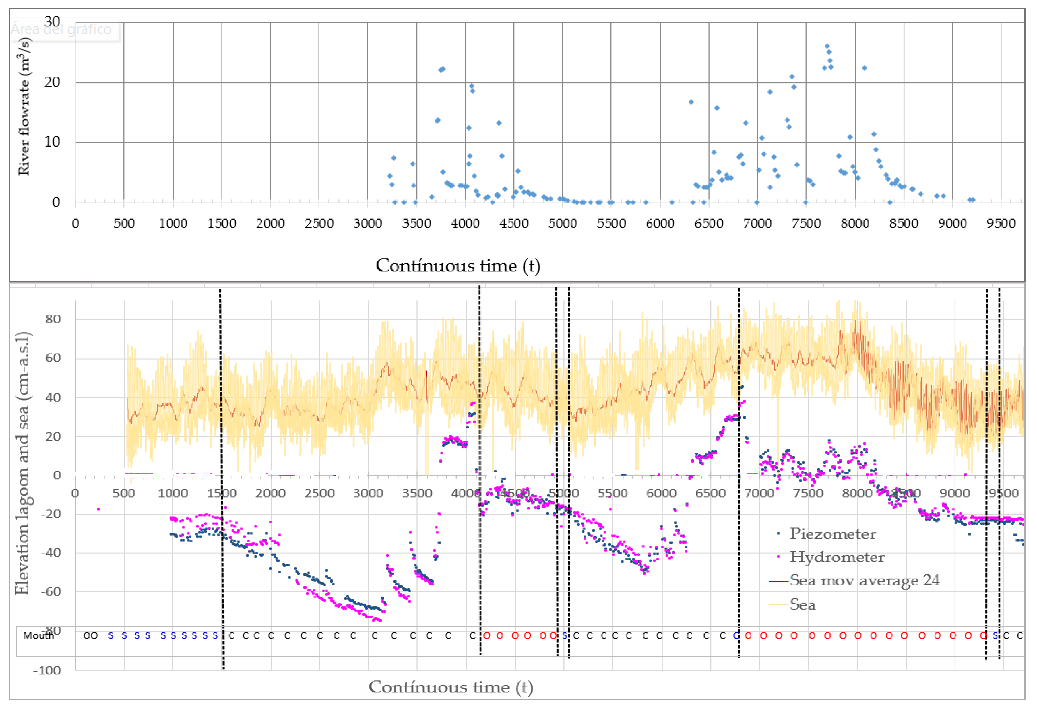

Table 1.
Consistency check between DEM output and measurements of lagoon elevation (“Area satellite I” is the area of the surface identified by satellite image and II after eliminating the holes left by the process; “Y Lag Topo-Bati” is the corresponding elevation determined through the y(S) relationship; “when” discerns the two daily measurements of the piezometer (“Y Lag Piezometer”) and of the hydrometer (“Y Lag Hydrometer”); “Y Lag measured” is the selection between the two according to the threshold -0,2; “Diff” (Y Lag Topo-Bati - Y Lag measured) is the deviation.
|
Date |
Area |
y Lagoon Topo-Bati (m.a.s.l) |
When |
y Lag Piezo (m.a.s.l) |
y Lagoon Hydro (m.a.s.l) |
y Lag measured (m.a.s.l) |
Diff (cm) |
| (m2) | |||||||
| 2023-05-02 | 4,949,302 | -0.707 | morning | -0.711 | -0.770 | -0.711 | 0,004 |
| -0.707 | afternoon | -0.700 | -0.772 | -0.700 | 1,407 | ||
| 2023-03-15 | 8,484,668 | -0.540 | morning | -0.593 | -0.653 | -0.593 | 0,053 |
| -0.540 | afternoon | -0.596 | -0.652 | -0.596 | 0,056 | ||
| 2022-05-31 | 13,673,330 | -0.241 | morning | -0.084 | -0.089 | -0.089 | -0,152 |
| -0.241 | afternoon | -0.156 | -0.161 | -0.161 | -0,080 | ||
| 2022-09-20 | 17,554,393 | 0.263 | morning | 0.446 | 0.367 | 0.367 | -0,104 |
| 0.263 | afternoon | 0.451 | 0.365 | 0.365 | -0,102 |
Disclaimer/Publisher’s Note: The statements, opinions and data contained in all publications are solely those of the individual author(s) and contributor(s) and not of MDPI and/or the editor(s). MDPI and/or the editor(s) disclaim responsibility for any injury to people or property resulting from any ideas, methods, instructions or products referred to in the content. |
© 2024 by the authors. Licensee MDPI, Basel, Switzerland. This article is an open access article distributed under the terms and conditions of the Creative Commons Attribution (CC BY) license (http://creativecommons.org/licenses/by/4.0/).
Copyright: This open access article is published under a Creative Commons CC BY 4.0 license, which permit the free download, distribution, and reuse, provided that the author and preprint are cited in any reuse.


