Hydrological Modelling of the Navio-Quebrado Coastal Lagoon (La Guajira, Colombia): A Challenging Exercise

1. Introduction

Coastal lagoons are delicate environments governed by energy, nutrients and, first of all, water exchanges amongst, mainly, the atmosphere (precipitation and evaporation), the river basin (fluvial freshwater inputs) and the sea (tidal water exchange). A hydrological monitoring exercise has been conducted in the coastal lagoon Navio-Quebrado (Colombia; [1] and the obtained data allowed us to set up a simulation model useful to understand its dynamics by firstly replicating quantitatively its behavior during the recorded period. Such a model can then be used to investigate about future scenarios under climate change; indeed, a key question is about what will happen to the lagoon with a modified fresh water input from the feeding river, a different (increased) evaporation rate, a different pattern of precipitation, a changed morphology of the lagoon (possibly undergoing a sedimentation process) and a risen sea level.

Another lower-level, more technical issue concerns the assessment of strengths and weaknesses of 0D hydrological modelling (dynamic water balance) with respect to a hydrodynamic 2D model: these two tools are here compared in critical terms to provide hopefully useful hints.

In the cited previous paper [1] on the monitoring system the different components have been presented which will be recalled in what follows.

This paper starts with a position on the system schematization where the relevant variables are introduced. We hence define all the factors relevant for a hydrological model of the lagoon (basically a water balance). Then some important aspects of how missing information has been dealt with to set up a complete and consistent dataset to feed the model are provided. Some structural key differences between the 0D and the 2D models adopted are then pointed out. Results are finally presented and discussed for both the simplified and the full model and conclusions derived.

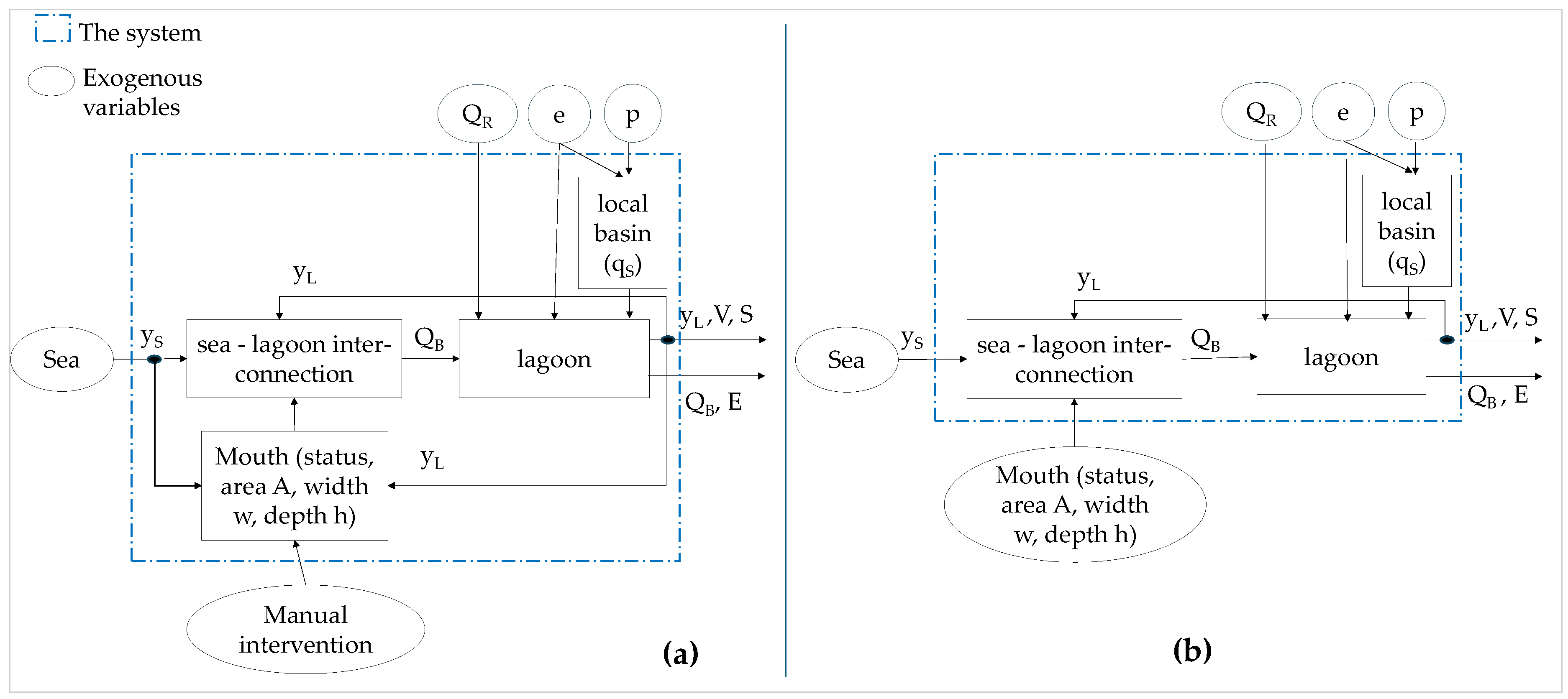
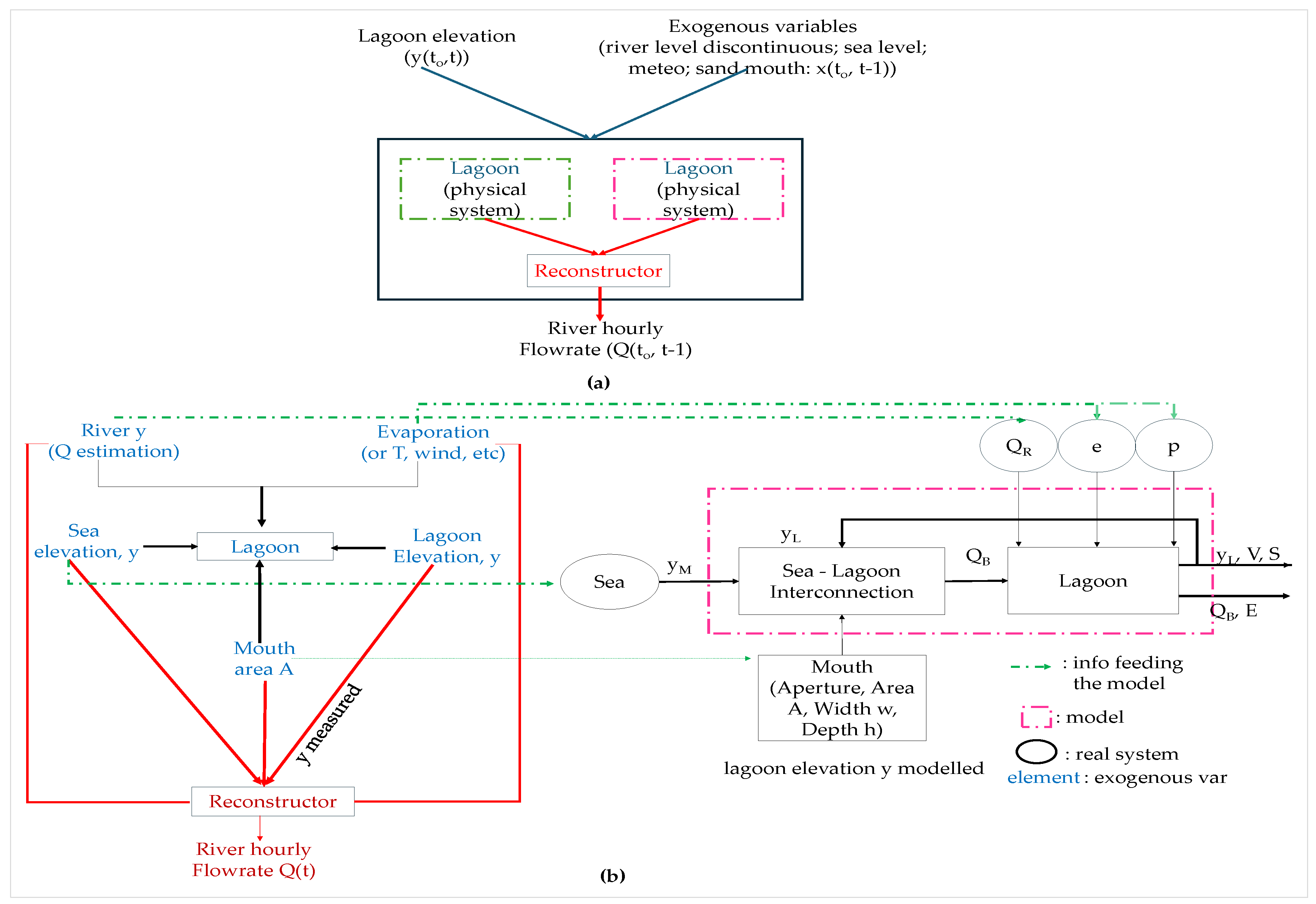
2. System Approach: Two Views of the Same System

As shown in the system sketch of Figure 1a, the hydrological dynamic system “Navio-Quebrado (alias Camarones) coastal lagoon” is subject to a number of exogenous, uncontrollable (or “natural”) input variables, namely: the fresh water inflow from the main river basin Tomarrazón-Camarones; the precipitation p determining the direct inflow input on the water surface S(t) and the runoff q(t) from the local watershed; the climatic variables determining the evaporation rate e(t) (and the evaporation flow E(t)=e(t)S(t)) and the sea level (yS), governing the water exchange with the sea. There is also a human-induced variable, treated here as an exogenous variable: the occasional manual modification of the lagoon mouth. This intervention is sometimes carried out to lower the lagoon’s water level when the mouth has not naturally opened. This latter input affects the dynamic block of the “boca” (i.e. the mouth) that periodically opens, grows, then shrinks and again closes so governing the mouth cross-section area A(t). This complex dynamic behavior is dependent on the elevation yL of the lagoon water surface and that (yS) of the sea. These two variables, together with the cross-section A(t) of the mouth, and possibly other factors (wind, salinity,...) determine the water exchange QB(t) between the sea and the lagoon (positive, when outgoing, or negative, when entering the lagoon).

The system has hence two state variables: the storage volume V(t) and the cross-section area A(t) of the boca. The dynamic behavior of the storage is relatively simple, given all the flows affecting it, as it is a straightforward dynamic water balance. Clearly, a key component is the morphological characteristic of the lagoon shelf, that is, its volume-elevation relationship V=V(yL), as well as its area-elevation relationship S=S(yL).

The dynamic of the boca cross-section is much more complicated: in a dry period, it closes completely because of a sand bar set by the sea waves in front of it; then, it comes the time when it opens again, usually after a significant river flood that rises the level over a given threshold (but sometimes locals intervene manually to “help” the process or sometimes it is the sea that rises anomalously and opens from the outside); then it remains opened for several weeks or months allowing for an alternate lagoon-sea water exchange depending on the tide; and then it shrinks and closes again when the freshwater input drops. This process is often, but not always, repeated twice a year according to the bimodal climatic pattern.

A much more simplified version of the Camarones lagoon system, with just one state variable (the storage), is presented in Figure 1b. This version simply ignores the dynamics of the boca that hence must be specified as an exogenous variable. Clearly this is not suited for the simulation of future scenarios, but it is very well suited to calibrate the core hydrological block (the storage dynamics) by using historical data, i.e. a record of opening and closing sequence of the boca.

Notice that up to now we referred to the “mono dimensional” and “bi dimensional” attribute thinking of the system concepts of number of state variables (one for the simplified version, two for the full version). But both versions can also be classified with regard to their spatial dimensions: the scheme can actually be 0D, when no spatial direction of flow is actually considered (i.e. the lagoon is just a tank, filling and emptying), or 2D when a movement of water in the horizontal x,y directions is considered. The 0D case is managed here as a discrete time dynamic system; while the 2D as a continuous time dynamic system discretized in both time and space.

3. Elements of the Modelled System

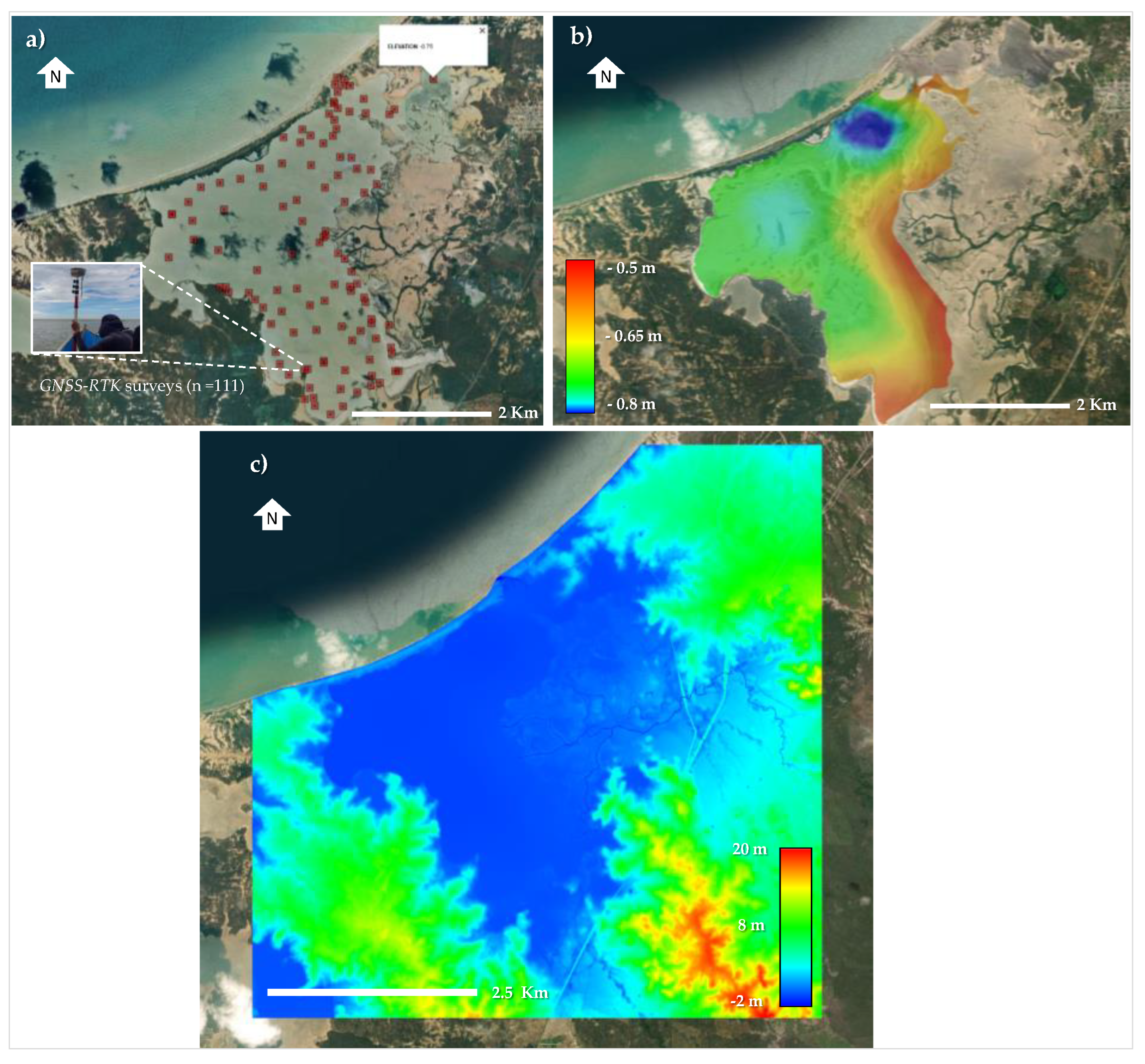
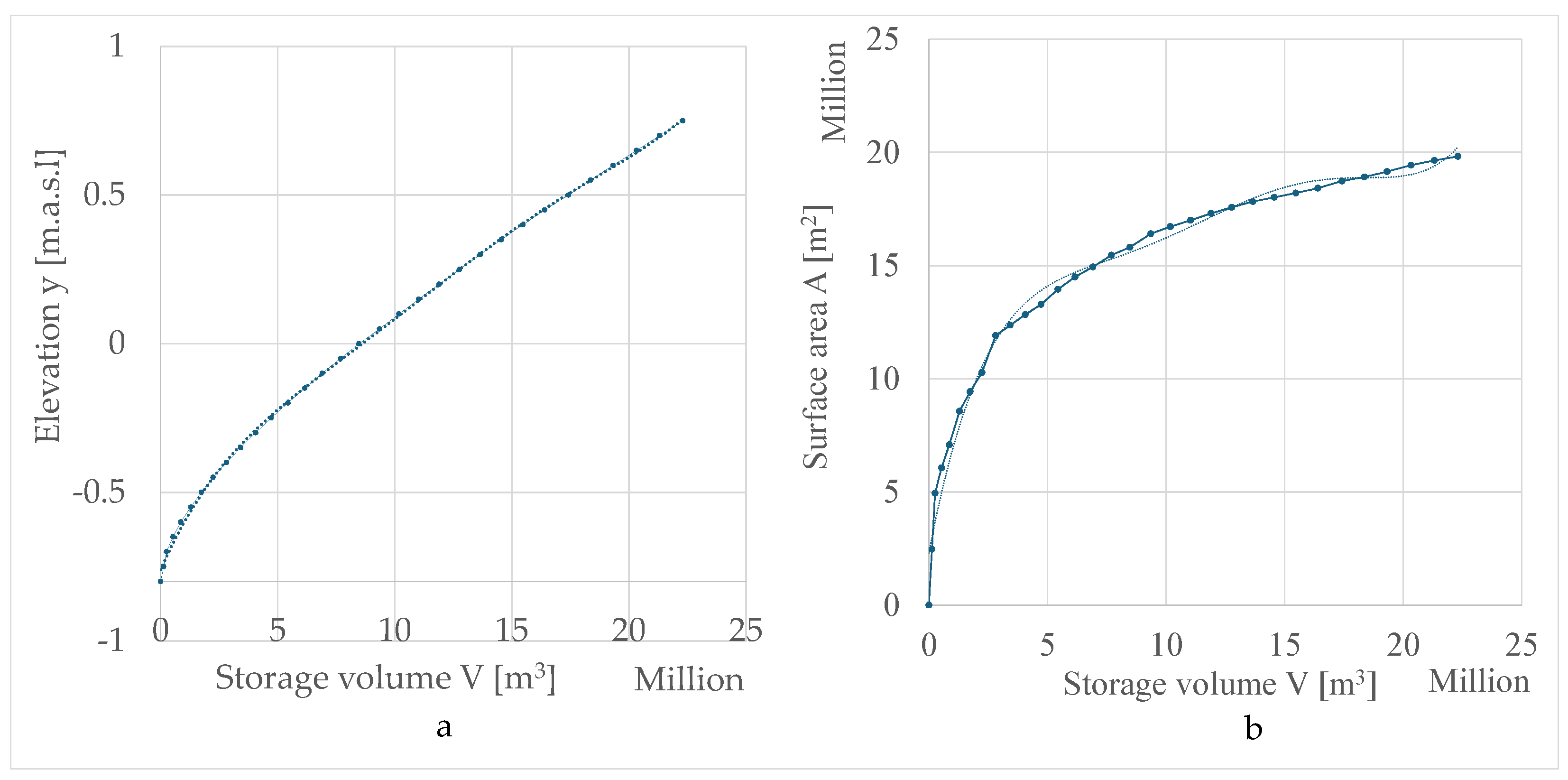
3.1. Morphometrics

The purpose of this analysis was to obtain an area-elevation relationship (curve A(y)) and associated storage-elevation relationship (V(y)) for the lagoon. This includes a bathymetric part (under water) and a topographic part (under the open air), varying of course with the particular moment considered. We relied on three types of data: i) a set of available large-format aerial images captures with a Vexcel UltraCam large digital camera; ii) sporadic data from our survey in situ with a RTK along the limits water-shore and on the bottom (Topcon HiPer V Dual Frequency GNSS Receiver, n= 93 along the shore, n= 111 on the bottom); iii) a sonar survey of the lagoon shelf (Garmin STRIKER™) with 2 transects and a total distance of 12.6 km, while lagoon width is about 3.3 km and its length 3.9 km, hence a point density of 41 points per km2). In addition, an already installed hydrometer recorded the elevation of the water surface referred to the average sea level reference adopted. This latter has been used as a validation tool, as explained further ahead. Figure 2 shows the three steps process adopted to generate the topo-bathymetric Digital Elevation Model (DEM) of the whole lagoon, including its floodable areas (dry at the moment of the survey).

Basically, altimetric data of the floodable area obtained from a crewed aircraft via photogrammetric reconstruction, were integrated with topo-bathymetric data obtained from a survey in situ.

3.1.1. Process

Firstly, we generated the bathymetric surface by interpolation of (orthometric) data obtained with the GNSS-RTK system (n = 111 points, Figure 2a), from a boat; these data, linked to the local geodesic network, were taken on September 19 and 20 of 2022 (Datum MAGNA-SIRGAS central and geoidal model GeoCol2004). Secondly, these data were processed in GIS (Geostatistical Analyst-ArcGIS Pro packed) via kriging interpolation. Thirdly, smoothed elevation curves were extracted that allowed the construction of a Terrain Digital Model in a form of a Triangular Irregular Network (TIN) as adherent to the flat lagoon bottom as possible (Figure 2b). Lastly, this TIN was converted into a bathymetric raster and integrated with the points cloud from photogrammetry so obtaining the desired topo-bathymetric DEM (Figure 2c) with a 1 m spatial resolution.

The photogrammetric points cloud is the output of the processing of georeferenced images obtained with a pixel size expressed in ground or Ground Sample Distance (GSD) image of 20 cm/pixel, taken by the governmental agency Fondo de Adaptación during March 2017.

Finally, the surface-elevation curve A(y) and the volume-elevation curve V(y) were built from the topo-bathymetric DEM by using the r.lake.xy module of GRASS_GIS ([2]).

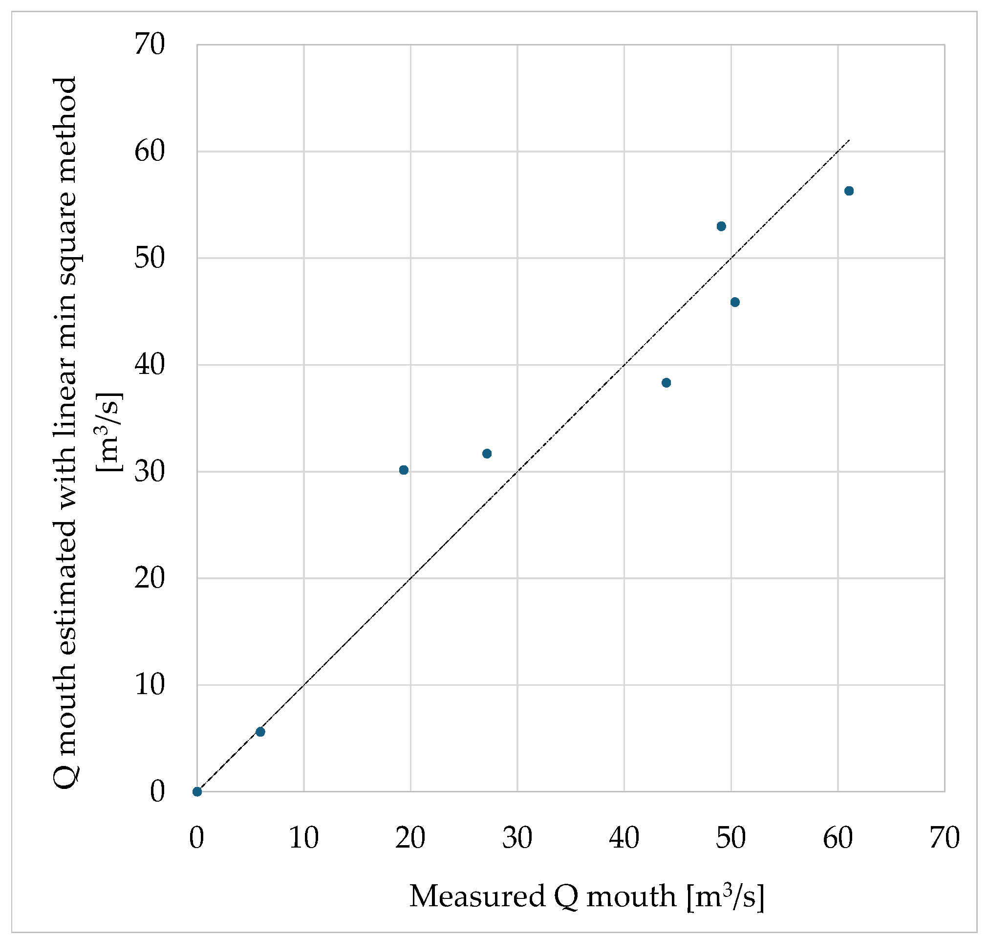
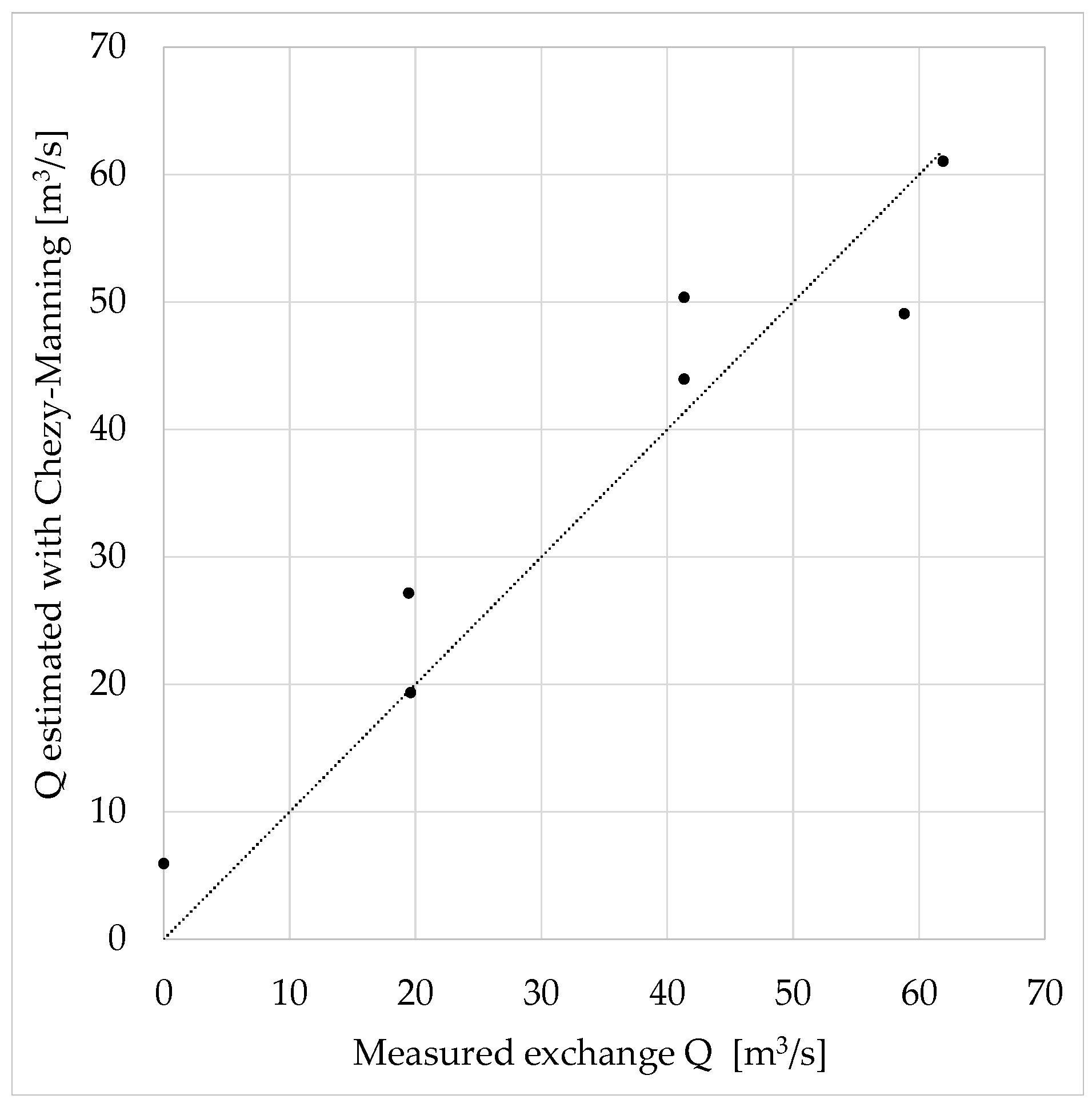
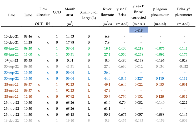
3.1.2. Validation

A checking of our DEM elevations in the dry floodable areas around the lagoon, via a survey carried out with GNSS-RTK (n=93) during a posterior dry season (March 13, 2023), reveals an altimetric average error of 3 cm and a RMSE of 32 cm. As this metric is smaller than 2 times the GSD, we concluded that the absolute precision of our DEM in those areas is satisfactory.

Independently, during the bathymetric campaign, we obtained data of the lagoon depth through a sonar (Garmin Striker) in order to validate the DEM generated, by comparing the values in n = 532 points. The raster map of depths from the topo-bathymetric DEM has been calculated again with the r.lake.xy tool of GRASS GIS, taking as a reference the water mask obtained from a Landsat 8 image of the same day of the campaign. The average error of 11 cm and the RMSE of 21.2 cm speak of an acceptable consistency.

A final validation check was performed by using the A(y) curve and comparing the elevation obtained from it, for a given area A, with the elevation provided by our hydrometer [1]. We considered four different situations of the lagoon; for each one, a water mask was extracted from Sentinel 2 satellite images (EOS Land Viewer Web Interface for Land/Water band combination: https://eos.com/landviewer : May 2, 2023; March 15, 2023; May 31, 2022 and September 20, 2022) . We obtained a satisfactory RMSE of 8.4 cm [1], what supports us in assuming that the obtained model can reliably be used for modelling purposes.

As a final step, we obtained two further relationships needed for modelling purposes: elevation-volume y=y(V) (Figure 3a, equation 1); and area-volume A=A(V) (Figure 3b, equation 2).

y = 1.32E-36x⁵ - 8.37E-29x⁴ + 1.98E-21x³ - 2.22E-14x² + 1.79E-07x - 7.60E-01

(1)

A = 6.11E-29x⁵ - 3.82E-21x⁴ + 8.95E-14x³ - 9.81E-07x² + 5.46E+00x + 2.31E+06

(2)

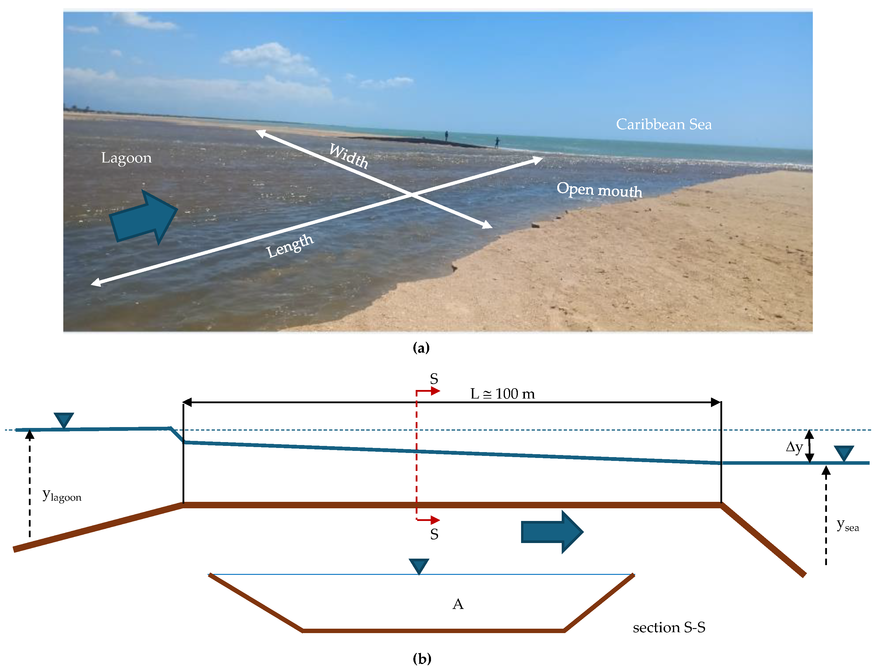
3.2. Mechanisms: Lagoon-Sea Exchange Flows

The idea is assuming that the exchange flow be governed by the height difference (yL-yS) between lagoon and sea (Figure 4), and the size of the cross-section area A of the boca (given as exogenous data), while other possible factors (e.g. shape of the cross-section, wind, salt concentration gradient,…) are ignored. Of course, the flow would be outgoing (lagoon into the sea) when the difference is positive and vice versa incoming (from the sea into the lagoon) when negative.

When looking for a relationship of the type QB = QB(yL, yS), we encountered an inconsistency as already mentioned in [1], apparently it always resulted yL << yS as shown in Table 1, which is physically impossible and most probably is due to a mismatching of the reference elevation adopted. Therefore, we looked for a constant ϕ that, once subtracted from the P.Brisa sea-gauging station data, provided a consistent height difference. We proved that with ϕ = 0.618 m all cases, except one, became consistent (see Table 1). Plotting the Q data with the height difference reveals a meaningful relationship particularly when data are separated into two groups according to the size of the cross-section (not shown for simplicity); this is indeed quite reasonable because the flow must be larger for a larger cross-section.

A simple multiple, linear regression, linking the flow rate QB to the height difference (yL - yS*) and to the cross-section area A (Equation 3 y 4), provides a nice performance (other non-linear relationships can certainly improve this result):

QB= QB (yL , yS, A)

(3)

QB= [k1 (yL - yS*) + k2 A + k3]⁺

(4)

where: QB denotes the exchange water flow [m3/s]; the symbol yS* denotes the corrected sea level datum, that is: yS* = yS - ϕ, with yS the elevation measured at P.Brisa tide-gauge station and ϕ = 0.618 m; [x]+ denotes the absolute value of x;

and: k₁ = 94.6528; k₂ = 0.6150; k₃ = - 6.7008; ϕ = 0.618 m are calibrated parameters.

Figure 5 shows the matching between the measured flows and the estimated ones through Equation 4 which we consider satisfactory, given the rude methods adopted and other uncontrollable factors affecting the outcome (e.g. distance of P. Brisa from the lagoon mouth; presence of wind; etc.). Of course, the relationship is fully valid only within the range of values utilized in its calibration.

To strengthen the quite surprising results obtained, we went through a completely independent verification of the obtained relationship, by applying classic hydraulic concepts. We schematized the boca as a short channel where flow would be governed by the typical Chezy-Manning equation [3], with a length of 100 m and a slope given by the height difference of Table 1 over such length (Figure 4b).

With a calibrated Manning coefficient n=0.040, the consistency of the found values is, once more, surprisingly nice (Figure 6) (we are aware that, for instance, the flow is not uniform and the actual gradient is lower because of the initial acceleration).

As a conclusion, the relationship (Equation 4) found by multiple, linear regression seems well suitable to represent the flow exchange. It adopts as exogenous variable the sea elevation, while the lagoon elevation is a state variable of the dynamic system; but it also needs the cross-section area A so that a rule to describe its evolution as a function of the other variables needs to be defined and is discussed in the following paragraph.

3.3. Mechanisms: Dynamics of the Mouth

The challenge here is to achieve an explanation of the dynamic of the boca in terms, first of all, of its process of opening and closing, and then in terms of cross-sectional area. Without this understanding it is virtually impossible to carry out long term simulations of future scenarios. Developing a credible theory for this dynamic behavior allows us to pass from scheme a) to scheme b) of Figure 1.

From the few observations we have got during our monitoring period (December 10, 2021 - June 30, 2023) it seems legal to infer (Figure 7) that the boca opens when either the lagoon water surface elevation or the sea elevation passes a threshold ϑ₁ (approximately 0,35 m asl). Then, it keeps open for at least a minimum interval τ_min (about 1,5 months) unless one of the following two conditions occur:

- a time superior to the maximum openness duration τ_max elapsed (about 4 months)

- the lagoon level drops below a minimum threshold ϑ₂ (about -0,24 m asl) and the maximum height difference between the lagoon and the sea is below the threshold σ (about 12 cm), i.e. there is enough little energy for the sea to re deposit the mouth bar that closes the lagoon.

Implementing this rule provides a quite nice reproduction of the pattern historically observed during our monitoring, as visible in Figure 7, although the duration does not perfectly coincide with the (supposedly) observed one. No guarantee, however, can be given that this “model” actually behaves reliably well for other periods. Further data will be gathered to explore its validity and possibly modify it suitably.

The dynamic of the cross-section area A is assumed to adhere to the following rules:

- from when it opens, it increases linearly, but quickly (τfull = 5 days) from 0 to the maximum Amax (this in principle could depend on the strength of the opening process, but this is influenced in turn by the human intervention, not recorded up to now, so at the moment it is not possible to establish a relationship); the maximum value recorded is here adopted (Amax = 92 m²)

- then it keeps more or less constant for a certain interval τkeep (about 20 days)

- then it diminishes exponentially until the next closure instant.

The results of applying this “theory”, together with the pattern reconstructed (extrapolated) from the few available measurements, is plotted in Figure 8. It is evident, that some additional mechanisms need to be incorporated in order to modulate the maximum area values, but this needs to wait for further observations and data.

3.4. Inflow from Runoff and Direct Precipitation

We assume that the precipitation over the area usually occupied by waters directly flows into the lagoon, even when it shrinks; but not all of it translates into an actual surface water flow because i) part of it evaporates before it touches the ground; ii) the available data refer to Camarones station (latitude 11°25'43.75", longitude 73° 3'9.83", see [1] and, given the type of meteorological events occurring in the area, certainly cannot be assumed to spread uniformly above the lagoon area. Therefore, a reduction factor μ1 is needed and the equation is (Equation 5):

Q_p [m³/day] = μ₁ p S/1000 [m³/day]

(5)

where S is the lagoon max surface [m²] (directly observed from aerial photos) and p the daily precipitation at Camarones gauging station [mm/day].

To determine the flow generated by direct runoff from the local water basin (see [1]), a kind of hydrological rainfall-runoff model is needed. As a first, basic step, we assume that there is no significant delay nor accumulation so that a constant fraction μ₂ of the precipitation over the surface S_R of such basin (excluding the lagoon itself already accounted for) enters the lagoon; hence the flow is (Equation 6):

Q_R [m³/day] = μ₁ p S_R /1000 [m³/day]

(6)

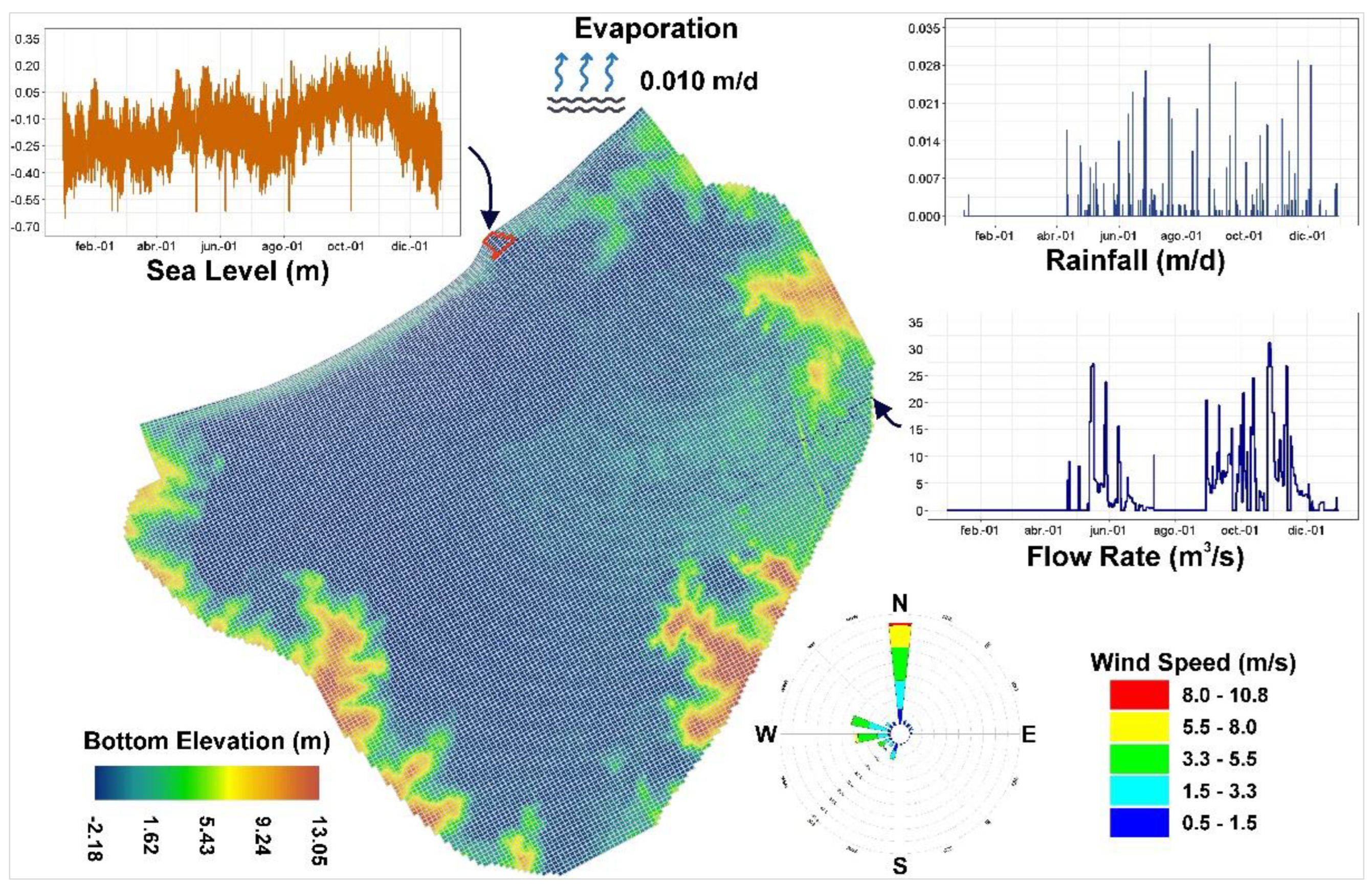
3.5. Evaporation

The evaporation flow from the free surface of the lagoon is determined as expressed by Equation 7 and 8:

e(t) [mm/day] = e (constant)

(7)

E(t) [m³/h] = S(t) * e(t)/(24*1000)

(8)

where E(t) is the evaporation flow from the lagoon in the interval (t, t+1); S(t) [m²] is the lagoon surface at time t, as evaporation is directly linked to the actual water surface present; and e(t) is the daily evaporation rate [mm/day] depending in principle on the specific climatic conditions of that day t. To determine the evaporation rate e(t) several formulas can be applied; their use is however limited by the meteo-climatic data available. As the temperature excursion is very limited in the area (less than 2.0 Celsius for instance in the period 01/10/1985 a 28/03/2020, while no data are available for our period), evaporation varies very little and mainly with wind, not available for our period. As a preliminary approximation, we adopted therefore a constant value of 10 mm/day, consistently with previous works [4].

4. Modelling of the Lagoon

4.1. Characteristics

4.1.1. 0D Spatial Modelling

The “0D” denotes here, as already said, that no spatial dimension is considered: the lagoon is seen as a tank. Additionally, thanks to the simplifying position of Figure 1b, the system has only one state variable: the storage V(t); and modeling the dynamics of the boca is bypassed.

Such a model has of course limitations. The main one is that it cannot see the distribution of flows and depths across the water body. However, the almost omnipresent wind or breeze and the very low depth (mostly less than 1 m) ensure that the complete mixed schematization is acceptable, at least vertically. Possibly, the freshwater input from the river and the incoming exchange flow from the sea are more complex spatially. But, concerning the latter, we observed only once a situation where the mouth was split into two parts with both an incoming and an outgoing flows present in the two separate sections; so that situation certainly is more an exception than the rule.

Although the physical system lives in the continuous time t, a discrete time schematization, with a quite short time step Δ (an hour), is very likely to be acceptable and this is what we adopted (Equation 9):

V(k+1) = [V(k) + Q_R(k) + Q_p(k) + Q_L(k) - Q_B(k) – E(k)]

(9)

where k denotes the time step, and all the terms have already been introduced, but are recalled here (all expressed as m³/hour]:

V(k): lagoon water volume; Q_R(k): freshwater input from the Tomarrazón-Camarones River (exogenous input); Q_p(k): freshwater input (exogenous input) from direct precipitation on the maximum lagoon surface S; Q_L(k): freshwater input (exogenous input) from the runoff into the lagoon from its local catchment; Q_B(k)= Q_B(y_L(V(k)), y_S(k), A(k)): is the exchange flow lagoon-sea (positive when outgoing), completely determined once specified the lagoon surface elevation y_L which is a function of the volume V(k) at that time through the corresponding inverse morphometric relationship so that y_L= y_L(V); while the sea elevation y_S(k), and the cross-section area A(k) of the boca are once again exogenous inputs; E(k) = S(V(k)) e(k): evaporation loss from the lagoon depending on the area S(k) of its surface given, for any volume V(k), by the corresponding indirect morphometric relationship S= S(V); while e(k) is again an exogenous input.

In this schematization all the exogenous inputs, by definition, are completely known given the time k.

The approximation of this formulation does not lie in the fact of being discrete time, rather it lies in the way the terms are computed. Indeed, the approach adopted in Equation 9 is that known as the Euler method [5]; that is, given a continuous time system of the type given by Equation 10 (i.e. that describing the lagoon physical system):

dx(t)/dt = f(t,x(t))

(10)

the discrete time version is approximated as (Equation 11):

x(k+1) = x(k) + f(t,x(k)) Δ

(11)

where dx/dt is the total derivative of time variable x with respect to the continuous time t; f(t,x(t)) is the transition function and x(t) is the state vector of the system. Clearly this is in essence a rude approximation as the continuous state may indeed change (a little?) during the interval (t; t+1), while in the discrete version, the new discrete state vector x(k+1) is computed by disregarding such further changes as if x(t) remained fixed at time t.

Many other approximations exist still within an explicit schemes, like that of the Runge-Kutta method [5], or jumping to implicit schemes [5], more precise, but heavier computationally. The Euler method seems however, sufficiently precise in our case.

4.1.2. 2D Spatial Modelling

For water bodies such as coastal lagoons, where the vertical dimension is much smaller than the horizontal dimensions and the depth is relatively uniform, a 2D model, rather than a full 3D model, is a good cost-effective solution [6]. This kind of models represents well the hydrodynamic behavior by simulating the distribution of flows of water across the water body without the need to describe complex vertical stratifications [7,8]. Two-dimensional models have proven adequate in shallow water flow situations, significantly reducing computational time with respect to the full 3D equation [9].

In principle, they are able to provide extensive information: time series of relevant variables (velocity, depth, water quality), velocity fields and current patterns, sediment transport patterns including the representation of changes in topobathymetry due to erosion and sedimentation processes [10,11,12,13]. Such models can also simulate the opening and closing of the mouth of the lagoon, like in the case of in the case of our Navío Quebrado Lagoon, and finally, they allow the simulation and analysis of the impact of extreme climate events related to climate change.

A 2D model conceptually appears therefore more suited and attractive than a 0D. But the accuracy of numerical models is heavily reliant on the presence and quality of input data. 2D hydrodynamic models for coastal lagoons require indeed a series of detailed and specific input data to configure, implement, and produce accurate results. Among these inputs, topography, and bathymetry (topo-bathymetry) are fundamental since detailed information is required on the conformation of the lagoon bed, the marine area, and the surrounding terrain.

Taking a step back, starting with the simple water budget, a number of issues become hence relevant referring to our exercise. In particular, a first set of issues refers to the ability to reproduce the historical behavior (observed period):

Is it technically possible to model a time varying mouth according to a measured time series? (i.e. a mouth geometry treated as a known exogenous input; actually, an interpolated time series obtained from few, irregularly scattered measures of the mouth width):

▪

Models could dynamically adjust the size, shape, cross-sectional area, and other characteristics of the lagoon mouth based on input time series data as handled by the XBeach model [11,14]. But this exercise involves significant challenges and complexities [14,15].

▪

One simple way to deal with this is to adopt a (topo-bathymetric) DEM including the largest mouth, and then run a number of simulations, each starting with the final state of the previous one and including a border condition with progressively a larger width on top of the DEM mouth, while the mouth is widening and vice versa when it is narrowing. A more elegant solution is to embed directly in the model code (usually not accessible) a time varying border condition.

The answer anyway is hence “positive”, although not straighforward.

Is the 2D model able to reproduce the observed historical behavior (lagoon water level time series), while adopting the same input information utilized in the 0D exercise? (that is: river inflow, sea level, precipitation time series, mouth width and depth and constant evaporation rate).

▪

This implies that the model determines automatically the exchange flows across the mouth, given the sea level and the current lagoon water level. This seems quite feasible according to the very nature of the 2D model approach: at any time, in any cell of the discretization modelling grid, a gradient is computed and a corresponding flow determined (in x,y directions).

▪

Winds are crucial in the phenomena of coastal barrier overflow and favor water exchange between the lagoon and the sea (ebb and flow), so for the case at hand where winds are scarcely known, the 2D model output can be negatively affected.

The answer is therefore in principle positive, but assessing the actual output is a other story and deserves a check.

Is it possible to incorporate within the 2D model a formalized mechanism that determines mouth opening and closure? This is by far a more difficult requirement:

▪

In the 0D model we solved this by just including a very basic rule stating, essentially, that on top of a certain lagoon level (threshold), the mouth would open, while it would close below another threshold.

▪

In the 2D model, the mechanisms of bed morphology change can be embedded in the “physics” of the model itself, so that it autonomously and dynamically adjusts the mouth geometry in response to changing conditions, simulating sediment transport and morphological changes [15]. Several studies on lagoon barrier overtopping events have employed 2D hydrodynamic models to reconstruct the entire process and variability of water flows, including dam formation, breach flow hydrographs, and downstream flooding. This demonstrates the models' ability to capture complex morphodynamic and hydro-sedimentological processes [10,16].

▪

Obtaining however the data required by these sophisticated models (e.g., XBeach) is expensive and logistically challenging, limiting the model applicability in practical situations where data is scarce and generally unreliable [17,18]. In addition, sophisticated algorithms and robust numerical solutions [19] are required as well as specialized knowledge and experience to configure, run the model, interpret its results [14] and occasionally access to source code to perform the necessary adjustments and configurations to the computational algorithm. This level of expertise may not always be available, especially in resource-limited regions, further complicating the practical application of these models.

▪

To model in particular the closure of the mouth, essential input data detailing exogenous forcing inside the lagoon as well as in the marine domain (such as tide levels, waves, solids concentration and sediment transport by marine currents) are fundamental [11,16]. Without detailed, extensive, high-quality data input, hardly obtainable in general, as well as sufficient computational resources, the feasibility and accuracy of these types of models are significantly limited.

We can therefore conclude that, in particular, for the opening stage, the mechanism can possibly work, but it hardly could incorporate the fact that usually opening is supported by human intervention (the 0D model does not see this explicitly, but it does by just appropriately setting the threshold that already incorporates this human behavioral mechanism). For the closing stage, then, the exercise is by far more difficult because the model should incorporate the dynamic mass balance of the sea shore, including the mass transfer along the coast, as it is this input that, when waves prevail on the lagoon emptying process, build up the mouth bar.

In principle hence the answer may again be positive, but in practice it becomes quite challenging.

Finally, another big question deserves attention this time concerning the future:

is it possible to use the 2D model to simulate the lagoon behavior according to (several) long time horizons (and associated hydrological and sea level inputs)?

▪

Here the key issue moves on the computing and processing speed.

▪

Dimensionality reduction can be a way out (as explored for instance by [20]. However, especially concerning the simulation of coastal barrier breaches, significant computational resources are required due to the need for high-resolution numerical meshes and the complexity of the physical processes involved [13]. Mesh refinement in the breach area is generally required, implying an increase in computational cost as it necessitates decreasing the time step to maintain numerical stability. This can be a limiting factor, especially in the case of long-term simulations.

▪

Most probably, the answer becomes hence negative when dealing with a personal computer, while it may be positive when thinking of cloud computing [21].

To explore the practical feasibility to adopt a 2D model we proceeded with the EFDC+ Explorer software package because is a coupled model that solves hydrodynamics, contaminant transport, and water quality kinetics in surface water systems, all in one integrated code, eliminating the need for external coupling between the hydrodynamics and transport modules, with a combination of finite volume and finite difference techniques on a Staggered Cell type grid to solve fluid momentum equations [22,23].

In this study, EFDC+ was used to simulate hydrodynamics coupled with the temperature module to consider the atmospherics conditions, manly evaporation and precipitation. The EFDC+ hydrodynamic module solves the three-dimensional, vertically hydrostatic primitive equations of motion for turbulent flow in a curvilinear orthogonal coordinate system. It incorporates a second-order turbulence closure model, which relates turbulence viscosity and diffusivity to turbulence intensity and length scale. The model employs the state equation that correlates density with pressure, salinity, temperature, and suspended sediment concentration, enabling comprehensive simulation of complex hydrodynamic processes [24,25].

4.2. Replicating the Historical Data Set

The simulation period was established from January 20th, 2022, to June 30th, 2023. Covering several wet and dry periods, as well as incorporating the temporal variability that characterizes the dynamics of the lagoon due to the influence of multiple factors such as tides, winds, river flows and mouth opening/closing.

4.2.1. The 0D Case (Excel® Model)

In order to proceed with a simulation, once the model is implemented in a software (our 0D was made in Excel®), the harshest difficulty found is that the model needs a “continuous” time series of the river freshwater input; more precisely, it needs it on a discrete hourly time basis, but with no missing data. The reality unfortunately is that we can hardly count with few measures (actually, just estimations) of flow rate (gauging exercises). For the major part of the remaining time, instead, we only have one level measurement a day at an irregular time moment (usually between 6 am and 9 am, but sometimes even in the afternoon) at the chosen gauging station of P.Troncal (and that, closer to the lagoon, of P.Viejo, see map in [1]). But in both cases there is no information about what happened the remaining 23 hours of that day. Finally, this time series has “holes” because some days (not many indeed) no measurement was taken at all. A first easy step adopted was to transform the level measurements into flowrate data, thanks to the stage-discharge relationship obtained (see [1]).

Then, to “fill the rest of the day” we just assumed that the flowrate would remain more or less the same by just repeating the same measured or estimated value multiplied by a factor λ to be set by trial and error; this factor would in principle be smaller than unity in case the recorded value were a flood (because it is unlikely that the flood lasts several hours as the river basin is just about 500 km² and events are rapid), while it would be greater than unity in the case the measured value were a low flow case. In the application, one only value of λ was adopted for the whole time series. For days with no measurement, we then adopted the following reconstruction criterion: if the no-data period is one or two days, the reconstructed value is the average of the previous and following measured values; when the period is longer, the flow is null. This is consistent with the policy agreed with our partners that each time a flow was visible in the river, a measurement had to be taken, which implies that in all periods of no flow, no measurement is taken. It is clear, however, that the reverse statement is not necessarily true; this means that structurally it is expected that the river inflow be underestimated.

The sea level is measured on an hourly basis, so that no problem arises except the few days where a datum is missing in which case it is interpolated between the closest data. The level of the lagoon has been measured usually just twice a day (in the morning and in the afternoon), but this is not a problem because we use it just to compare the model answer with reality and assess its reliability, while the lagoon-sea water exchange module uses the state of the system (storage) calculated by model itself.

In the simplified version of the system scheme (Figure 1b) there is need to assign a time series of the status of the mouth (opening/closure and cross-section area); in the periods of “boca cerrada” (closed mouth) it is easy because A=0 and no exchange can occur; in the other periods we just interpolated linearly the few measurements available.

For the direct precipitation inflow and runoff from local catchment and the evaporation rate we just adopted the recorded time series of relevant meteo-climatic variables (temperature and so on) in a nearby station (see [1]).

4.2.2. The 2D Case (EFDC+ Model)

We discretized the domain area with curvilinear orthogonal horizontal coordinates. The grid was generated using the Curvilinear Grid Generator for EFDC (Grid+). The model has 203 elements in the X direction and 186 elements in the Y direction, with ΔX varying from 29.2 to 44.9 m and ΔY varying from 13.4 to 38.5 m, for a total of 25564 active cells (Figure 10). The topo-bathymetry of the study area obtained as described in Par.3.1 was processed into this high-resolution grid.

Atmospheric forcing data

A constant evaporation rate of 0.01 m/day was applied throughout the simulation time, consistently with the 0D exercise. Wind forcing was based on some measured wind speed and direction data available from February 1 to September 7, 2022, and kept constant throughout the period.

Initial conditions

The water surface was set at the level reported from the field measurements record. This implied the assumption of a horizontal water surface and no movement (v=0) everywhere.

Boundary conditions

The two main boundary conditions used were, consistently with what had been done for the 0D, a Dirichlet-type boundary for the discharge of the Tomarrazón River and a Neumann-type boundary for the connection with the sea, where sea level variation was imposed.

The river's boundary condition included the freshwater inflow from the main river basin Tomarrazón-Camarones and the runoff from the local watershed. Figure 9 shows the location of flow river boundary condition.

The boundary condition at the sea interface needs further clarification. To represent the closing and opening of the lagoon mouth, we use the time-varying field for bathymetry option available in EFDC+. This option allows to specify the time or spatially varying forcing factors for each cell over the whole model domain. By using this capability, EFDC+ can receive time varying topo-bathymetric updates within its computational domain from external sources. The area of the sand bar modified to reproduce the opening and closing of the mouth is demarcated with a red polygon in Figure 9. First, the topographic variation in the mouth zone was determined using the field measured mouth surface area (m2). To do this, a fixed width was established to obtain an approximated depth, then with the measured lagoon free surface level data this depth was converted into elevation above sea level. All the cells in that zone were modified by assigning a new bottom elevation each hour. Thus, a file with 527 different time-varying field for bathymetry was created to reproduce the behavior and variation of the mouth throughout the simulation.

5. Results

5.1. Results for 0D Model

Once suitable values of the parameters involved (reduction factor for direct precipitation μ₁ =0,5 and local runoff μ₂ =0,2; modulation factor of the river inflow λ =1,2) have been assigned (not through a formal calibration, but just an approximate trial and error procedure), the main results obtained are as follows:

▪

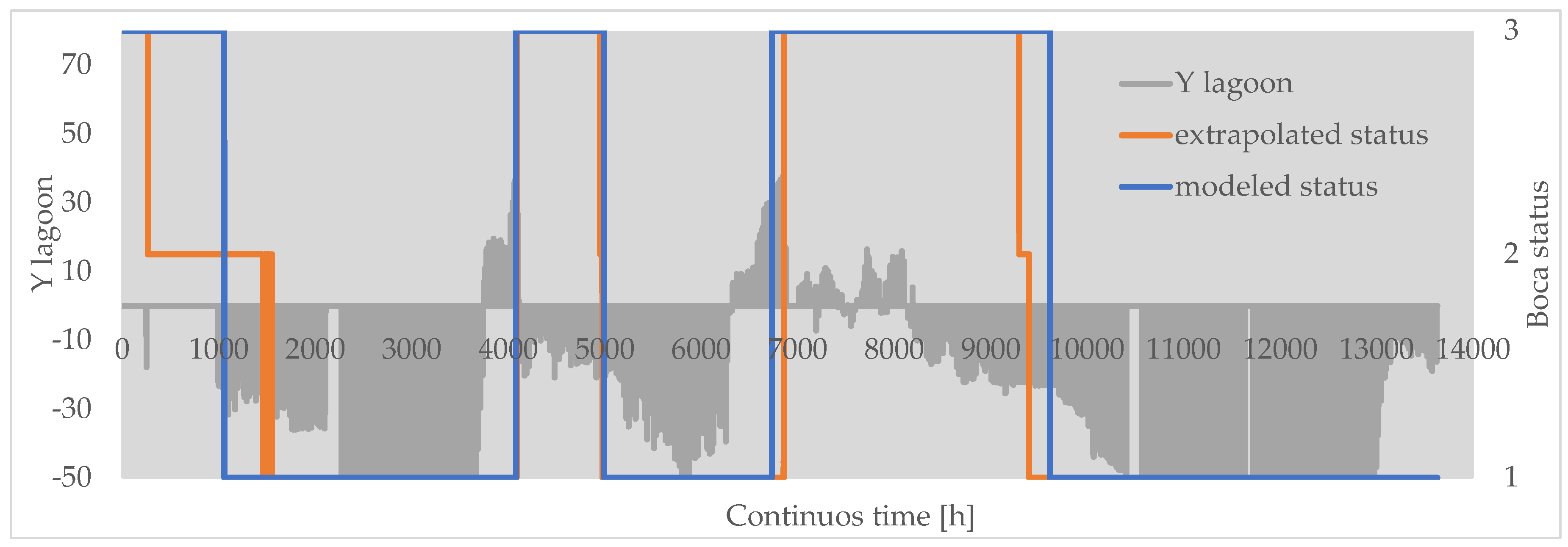
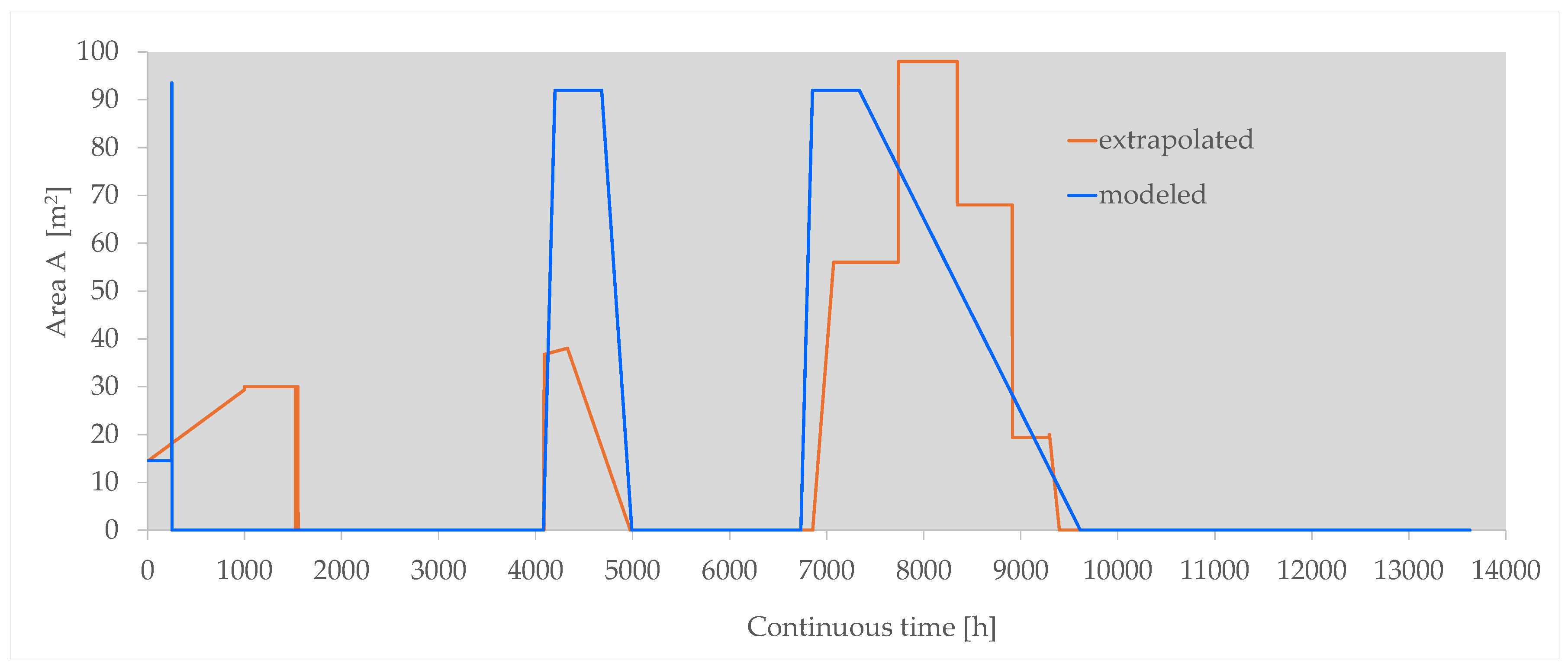
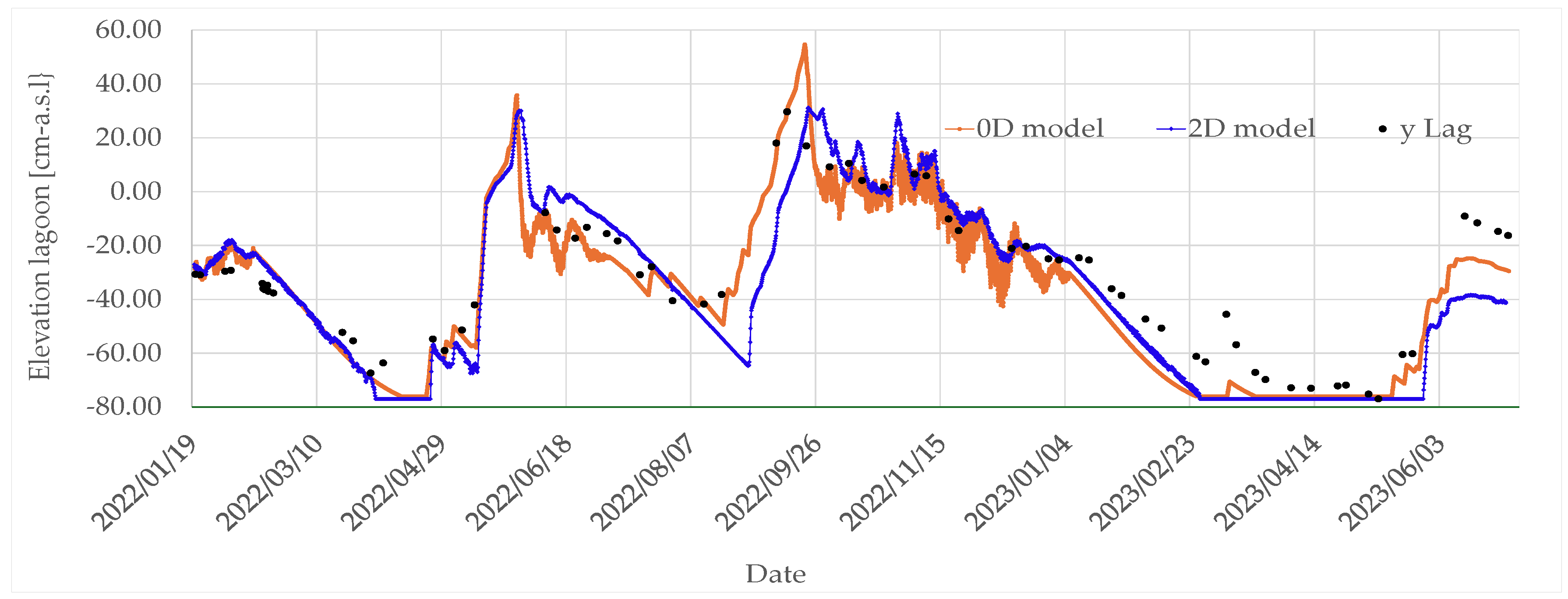
A thorough coherence with the general system behavior is evident (Figure 10)

▪

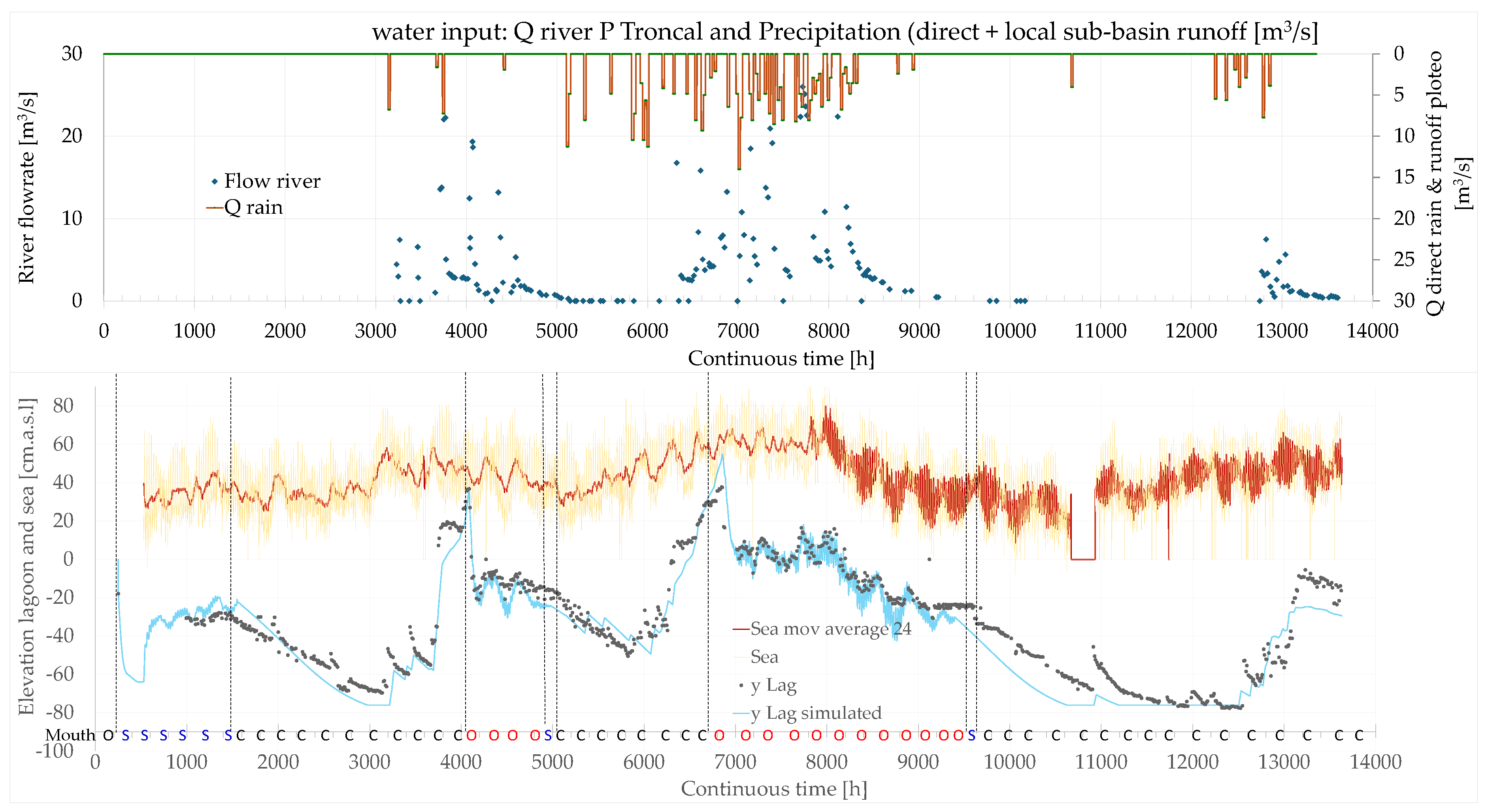
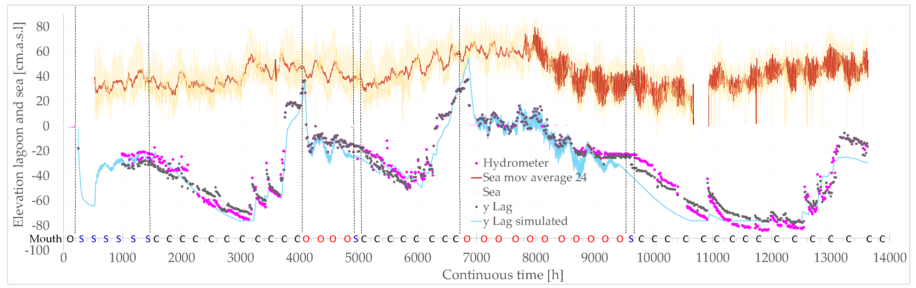
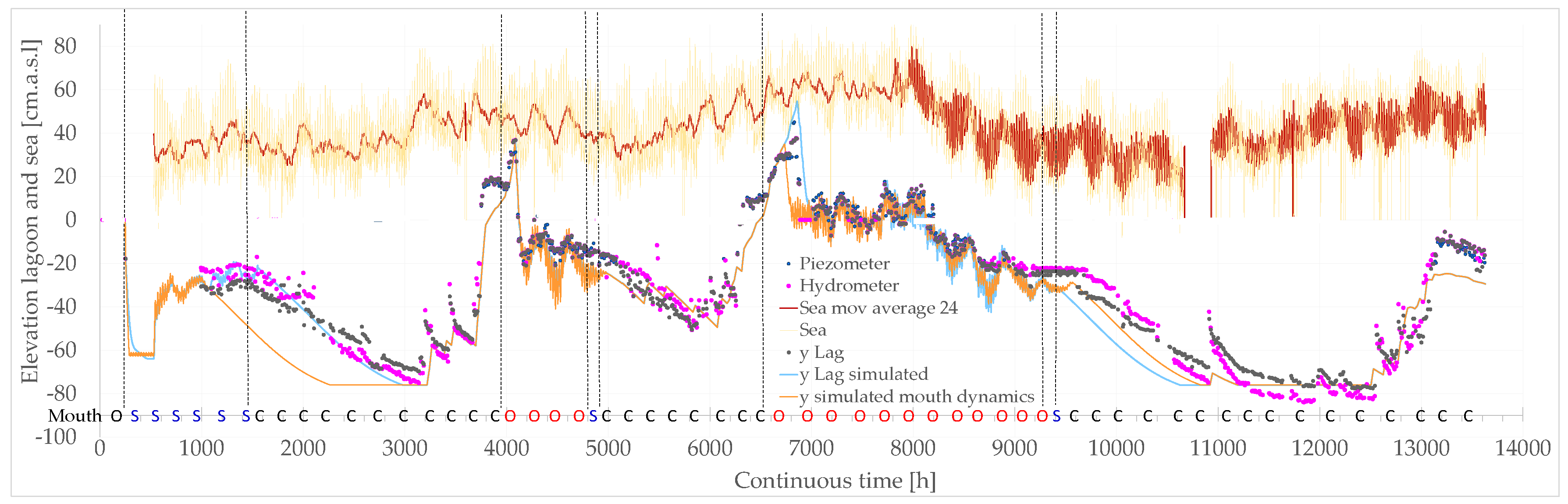
The model represents quite well measurements, although there is a general sub-estimation clearly due to lack of river inflow inputs (particularly between time 8300 and 11000, Figure 11) and a sporadic small overestimation, still lying between the hydrometer and piezometer data boundaries (notice that in the initial period until t=3000, the two instruments, hydrometer and piezometer, needed some adjustments and were less reliable).

▪

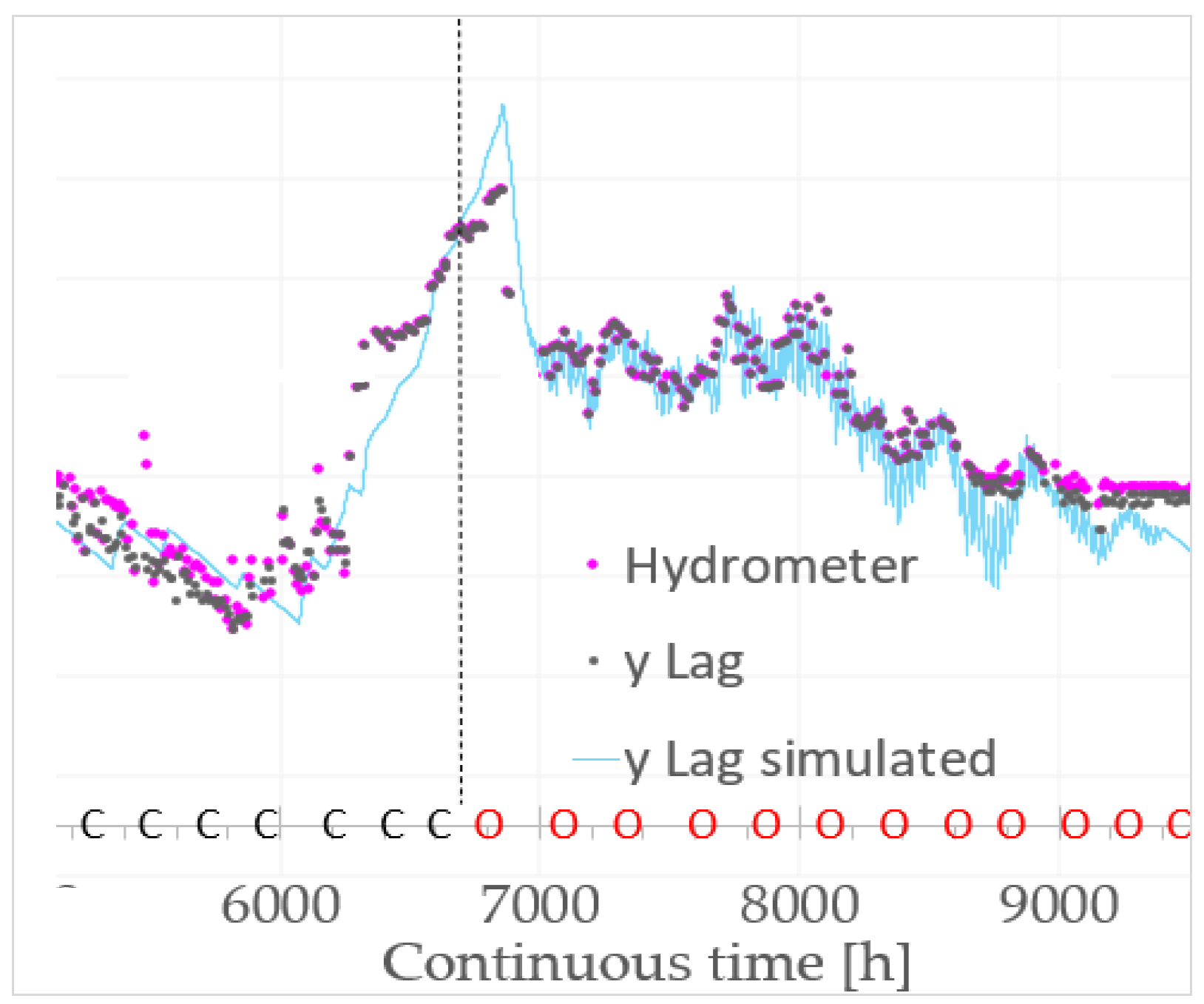
The tide is very “nervous”, with an amplitude of oscillations significantly larger than that of the lagoon; this is more linked to the 24h moving average. In addition, it is evident that between time 7000 until 9300 approximately, the lagoon elevation oscillation is much wider, but so is also the tide (actually its 24 h moving average value). In general, it must be considered that the lagoon elevation measurements only occur twice a day and hence, with such a low frequency sampling, it is very unlikely that the maxima and minima are indeed captured (Figure 12).

▪

There may also be calculation errors; indeed, the Euler method adopted structurally introduces some errors as, for instance, it determines the evaporation flow in the interval (k, k+1) based on the lagoon water surface (S(k) at time k, while it is constantly changing. Other errors may be due to an incorrect numerical representation of the morphometric relationships and to reckoning approximations.

▪

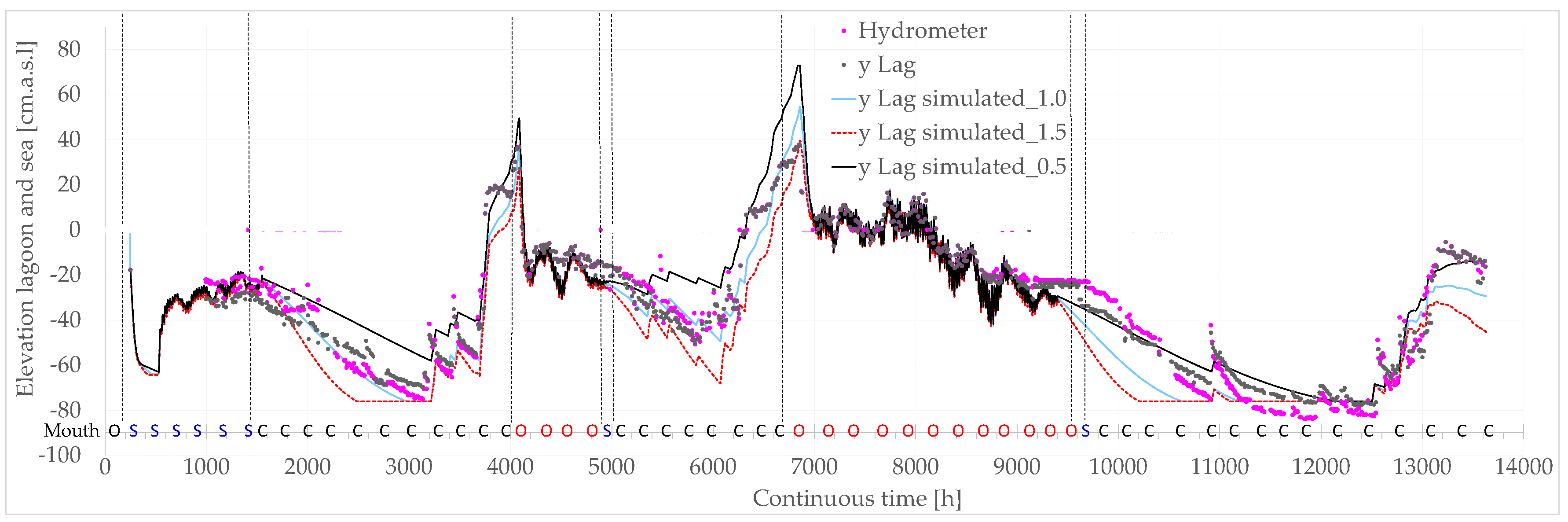
The system appears to be very sensitive to evaporation as shown in Figure 13. This means that more attention should be paid in the determination of the evaporation rate.

▪

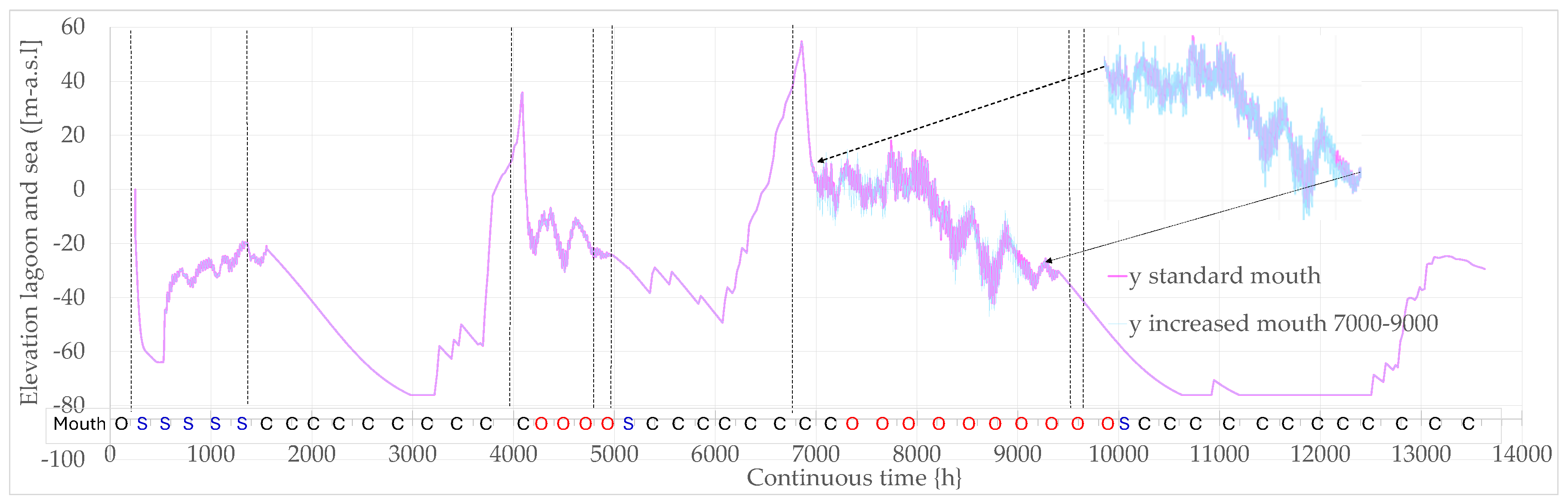
Finally, the cross-section area of the boca determines the amplitude of the water surface oscillations (and the associated flow rates), but not the general pattern of the elevation, as shown in Figure 14 for an increased value of 50% in the period 7000-9000 (as an example).

The Figure 11 to Figure 15 represents the findings. Notice that to allow discerning the lagoon elevation from that of the sea, this latter is reported without the shift correction (ϕ= 0,618 m) that instead the model sees; so, the sea graphs appear in the air, but have to be seen exactly shifted downwards of that quantity.

For the sea, the light dense line on the background is the actual sea level measured; the darker shorter amplitude line on top of it is its 24h moving average.

In Table 2 the water balance is reported for different time intervals. It is apparent that by far the major water input comes from the sea exchange; the river input covers the second priority, while evaporation is approximately double than the precipitation input.

It is worth noting that the mass balance shows a small error. This may be due to i) mutual inconsistency amongst the morphological relationships (the numerical V(y) is not really the integral of the S(y) as it should be) and numerical approximations adopted for their functional forms; ii) errors introduced by the Euler integration method; iii) approximations in the numerical reckonings (as it works at hourly time step, in a considered period of about one and a half year there are more than 13000 steps).

When the dynamics of the boca is incorporated (Par.3.3), results are a bit worse, but still acceptable, as shown in Figure 15. It is noteworthy that the main difference is an underestimation after the closure of the boca, particularly around time 1000-2500; this is due to the too early closure that impede a recharge of the lagoon by sea water. Additionally, the oscillations when the boca is open are in general a bit exaggerated. This latter problem can be solved by modulating the Amax parameter as already noted (see Figure 9); the former problem may improve by adopting a less gradual reduction of the section after reaching the maximum opening (i.e. not the linear pattern adopted, but for instance an exponential one), but the main point is to capture the right closure and with our data set -where the initial data are lacking (particularly the river inflow and the sea level)- this is not possible. This can be addressed once the observation period will be further extended. On the contrary, around time 9500-10500 the full model (incorporating the dynamics of the boca) seems better than the partial one (adopting the extrapolated area based on measurements); this is due to the opposite fact: the closure of the boca occurs later and so an increased volume from the sea can fill the lagoon.

A final observation is that the full model answer perfectly coincides with the partial one (without the dynamics of the boca) in the periods right after the dry out (time 3000 and 11000): this is where the system memory is nullified and a new cycle begins.

5.2. Results for 2D Model

The comparative plot of the time series of water levels in the Navio Quebrado lagoon (Figure 16) which includes measured data and results from 0D and 2D models highlights the key differences between both modelling approaches. The observed fluctuations in water levels are clearly influenced by the temporary opening and closing of the mouth that connects the lagoon to the sea, as well as by the seasonal contributions of the Tomarrazón River. These factors constitute the most important external drivers affecting the dynamics of the lagoon, as they regulate both the water level peaks during periods of highest flow and the decreasing levels when the lagoon is isolated, and evaporation becomes the main mechanism of water loss.

Curiously, the 2D model shows an adequate fit at moments when levels in the lagoon suffers gradual changes or when there are no large fluctuations induced by intense external forcing, that is, during periods without sudden changes. It tends however to overestimate some peaks and has less detailed responses with smaller variations compared to measured data and 0D model.

Again, as expected, there is an underestimation of water level towards the end most probably due to “escaped floods”.

6. Discussion and Conclusions

6.1. Discussion

The exercise we conducted can be considered successful as both models replicate quite satisfactorily the patterns of the measured variables, when the dynamics of the boca is considered an exogenous input (i.e. known from observations).

This result may appear obvious as the system and the model are extremely simple; however, reconstructing the inputs is not a trivial exercise.

A little worse result is obtained when the mouth dynamics is explicitly modeled in the 0D; but it can certainly be improved and can be considered sufficient for exploring future scenarios.

The comparison between 0D and 2D hydrodynamic models unveils the strength of the 0D model: it performs slightly better than the 2D and is evidently much simpler. Possible reasons for this are: i) although the area of the mouth between lagoon-sea has been represented as varying, following the actual system information (exogenous input), its width has been assumed constant, while it should have been modulated as well; ii) the wind was assumed constant throughout the whole period, because of lack of detailed information, while certainly it is not, and this increments the actual evaporation.

Moreover, it is able to replicate the dynamics of the mouth, although in a not perfect fashion, while for the 2D this predictive exercise has not been undertaken and would certainly prove much more difficult (notice that we included the mouth dynamic -as an exogenous input- to replicate the historical data set, but we did not conduct the very prediction of the mouth dynamic, that instead was done for the 0D as explained in Par.3.3). Finally, even if this additional element could (theoretically) be incorporated, simulating very long time series with the 2D model would be a challenge owing to the computational burden.

Importantly, the 0D model enabled us to ascertain that our comprehension of the physical behavior was correct and actually added several pieces of information. For instance, we ascertained that the tide, although determining the major water exchange, does not affect the general time pattern of the surface elevation; a variation of the mouth cross-section area influences the amplitude of the oscillations, while it is its moving average that introduces some real forcing effect, but of course only when the mouth is open. The evaporation flow, although by far smaller than the sea exchange flow and the river inflow, is the governing factor when the mouth is closed and outside of the rainy season. Another finding, although to be ascertained with further data, is that the effective input from the precipitation (directly to the lagoon or indirectly through runoff from its catchment) is much lower than what could be expected from the recorded data, contrary to the initial intuition; the main reason for that probably is the non spatial representativeness of the data. Finally, or first of all, it is essential to determine the full river hydrogram otherwise an underestimation of the lagoon water surface elevation is unavoidable.

The 0D model can be used with future climatic scenarios to assess for instance the frequency of events of dry out and their duration, the frequency of opening and closure events or the duration of the lagoon-sea exchange-phase. All these statistics can be very useful to predict ecological consequences hampering both the natural value of the system and its provisioning ecosystem service.

On the other side, it is evident that the 2D model can be key when simulating water quality issues as horizontal mixing in a shallow lagoon is a complex process that the 0D model cannot reproduce at all. Indeed, 0D models present significant limitations because they treat the system as if it were homogeneous, leading to underestimate sometimes the magnitude of extreme events and to be temporally delayed under changing conditions, as reported by [26]. These characteristics make 0D models unsuitable for simulating phenomena that require high spatial resolution, especially when interactions with the environment vary significantly. Additionally, the flexibility offered by 2D models to handle complex geometries, particularly using curvilinear or nested grids, allows for higher resolution in areas of interest, improving the accuracy in the simulation of water accumulation and redistribution zones [27].

In this context, the integration of 0D and 2D models has been proposed as a hybrid approach to take advantage of the benefits of both methods. According to [28], this combination can provide a more balanced representation of coastal systems, allowing the use of 2D models to accurately simulate extreme events, while 0D models can be employed for more computationally efficient long-term simulations. This strategy not only maximizes the accuracy in resolving the most complex hydrodynamic processes but also optimizes computation time, which is especially relevant in complex environments such as coastal lagoons.

6.2. Conclusions

Before our model can actually be used to explore future climate change scenarios, even if disregarding the mentioned (very important) effects of sediment transport, several improvements have to be made: the dynamics of the boca needs to be better represented and consolidated; evaporation and precipitation need to be better estimated taking into account the spatial patterns of the climatic variables; the Euler computational integration scheme can be improved.

In terms of data acquisition, most importantly, a better method to measure the river input has to be put in place. Certainly, a more automatized gauging station [29,30] would solve our problem, but -as pointed out in [1] - unfortunately the local socio-cultural context ensures that such a system would have short life. For the purpose of modeling the lagoon, possibly no other solution is available. Satellite imagery methods are not applicable here owing to the small width of the river and the dense riparian vegetation.

An indirect approach, however, can be adopted: set up a hydrological rainfall-runoff model of the river basin based on satellite precipitation data (now available) and reconstruct the flowrate based on precipitation data. Then, the problem would be how to calibrate such a model as there exists no official systematic river flow gauging station in our basin. In principle, the low granularity flowrate data available from our own gauging station can serve the purpose; but certainly, adding more data up to the whole hourly time series of river flow data would offer a better resource.

But even a more empirical approach can be explored by observing that the quite primitive monitoring system set up, together with the 0D hydrological model developed, can be used to implement a reconstructor of the river flowrate hydrogram: the idea is that from the variations of the lagoon level not explained by the causal variables that can be easily measured (precipitation and evaporation and sea exchange), one can infer what river flow must have occurred for the model to fit the discrete measurements of the lagoon water surface elevation. In other words, the lagoon monitoring system plus the model constitute a gauging system for the river (Figure 17).

The most basic approach would be to write recursively Equation 9 starting from a measured value yL*(k) of the elevation at discrete time k, until the following measurement yL*(k+Δ) after Δ steps so obtaining an articulated non linear function of the type:

y_L^*(k+Δ) = g(k,y_L^*(k); u(k), u(k+1),…, u(k+Δ-1))

(10)

where the function g(∙,…,∙) is a combination of the recursive use of Eq.1.a and the inverse morphological relationship V=V(y), while [u(k), u(k+1),…, u(k+Δ-1)) ] is the set of the unknown values sought for, being u(k) the generic river inflow, while all other exogenous inputs are supposedly known and hence embedded in the g(∙,…,∙) function. This is a problem with one non-linear equation and Δ unknowns, which by construction has no unique solution (if any); this is not at all surprising, as we are here trying to estimate a high granularity input (the river hydrogram at a hourly level), from low granularity observations (the lagoon elevation measured discretely just twice a day), taking advantage of the fact that these variables are interlinked by the continuity equation. Adding the information related to the following measurement (or to all available measurements) does not improve the situation because a new set of unknowns is also added.

However, if the fitting is assessed not on a single value yL*(k) at each real-world time t, but on the whole set of measurements taken from the last good fitting model time k*(t) until current time t (e.g. with k*(t) located at the end of a significant period of no river inflows), and by introducing some reasonable, practical hypothesis about the shape of the hydrogram portion, there may be a chance that a reasonable solution be found. In any case that would be a much better estimation than…nothing. The discontinuous measurements at the gauging station may greatly help, although are not essential in principle. Rigid schemes like Kalman filter [31] (originally conceived to reconstruct the state, but likely to be extended to estimate model parameters – e.g. [32]- and hence even its inputs that can be seen as special time varying parameters) cannot be applied here owing to the irregular and discontinuous measurement protocol adopted for the lagoon (and even more for the river).

This is a new open challenge to explore further.

References

- Nardini, A.G.C.; Escobar Villanueva, J.R.; Pérez-Montiel, J.I. Hydrological Monitoring System of the Navío-Quebrado Coastal Lagoon (Colombia): A Very Low-Cost, High-Value, Replicable, Semi-Participatory Solution with Preliminary Results. Water (Switzerland) 2024, 16. [Google Scholar] [CrossRef]
- Nartiss, M.R. Lake.Xy Module.
- Chow, V.T. Open-Channel Hydraulic; McGraw-Hill, Ed.; New York, 1959; ISBN 978-0-07-085906-7.
- Corporación Autónoma Regional de La Guajira [CORPOGUAJIRA] Ajuste y/o Actualización Del POMCA Del Río Camarones y Otros Directos Al Caribe – La Guajira; Riohacha, Colombia, 2022.
- Young, D.M.; Gregory, R.T. A Survey of Numerical Mathematics; Ed. orig.: Reading : Addison-Wesley, 1972, Ed.; Courier Corporation: New York, 1988; Vol. 1. [Google Scholar]
- Moraru, A.; Rüther, N.; Bruland, O. Investigating Optimal 2D Hydrodynamic Modeling of a Recent Flash Flood in a Steep Norwegian River Using High-Performance Computing. J. Hydroinformatics 2023, 25, 1690–1712. [Google Scholar] [CrossRef]
- Mao, M.; Xia, M. Seasonal Dynamics of Water Circulation and Exchange Flows in a Shallow Lagoon-Inlet-Coastal Ocean System. Ocean Model. 2023, 186, 102276. [Google Scholar] [CrossRef]
- Torres-Bejarano, F.M.; Torregroza-Espinosa, A.C.; Martinez-Mera, E.; Castañeda-Valbuena, D.; Tejera-Gonzalez, M.P. Hydrodynamics and Water Quality Assessment of a Coastal Lagoon Using Environmental Fluid Dynamics Code Explorer Modeling System. Glob. J. Environ. Sci. Manag. 2020, 6, 289–308. [Google Scholar] [CrossRef]
- Tsanis, I.K.; Wu, J.; Shen, H.; Valeo, C. Environmental Hydraulics: Hydrodynamic and Pollutant Transport Modelling of Lakes and Coastal Waters. In Environmental Hydraulics; Tsanis, I.K., Wu, J., Shen, H., Valeo, C., Eds.; Developments in Water Science; Elsevier, 2006; Vol. 56, pp. vii–360.
- Gunasinghe, G.P.; Ruhunage, L.; Ratnayake, N.P.; Ratnayake, A.S.; Samaradivakara, G.V.I.; Jayaratne, R. Influence of Manmade Effects on Geomorphology, Bathymetry and Coastal Dynamics in a Monsoon-Affected River Outlet in Southwest Coast of Sri Lanka. Environ. Earth Sci. 2021, 80, 238. [Google Scholar] [CrossRef]
- Herrling, G.; Winter, C. Spatiotemporal Variability of Sedimentology and Morphology in the East Frisian Barrier Island System. Geo-Marine Lett. 2017, 37, 137–149. [Google Scholar] [CrossRef]
- Nienhuis, J.H.; Törnqvist, T.E.; Esposito, C.R. Crevasse Splays Versus Avulsions: A Recipe for Land Building With Levee Breaches. Geophys. Res. Lett. 2018, 45, 4058–4067. [Google Scholar] [CrossRef]
- Li, X.; Leonardi, N.; Plater, A.J. Impact of Barrier Breaching on Wetland Ecosystems under the Influence of Storm Surge, Sea-Level Rise and Freshwater Discharge. Wetlands 2020, 40, 771–785. [Google Scholar] [CrossRef]
- Elsayed, S.M.; Oumeraci, H. Combined Modelling of Coastal Barrier Breaching and Induced Flood Propagation Using XBeach. Hydrology 2016, 3. [Google Scholar] [CrossRef]
- Maicu, F.; Abdellaoui, B.; Bajo, M.; Chair, A.; Hilmi, K.; Umgiesser, G. Modelling the Water Dynamics of a Tidal Lagoon: The Impact of Human Intervention in the Nador Lagoon (Morocco). Cont. Shelf Res. 2021, 228, 104535. [Google Scholar] [CrossRef]
- Nienhuis, J.H.; Heijkers, L.G.H.; Ruessink, G. Barrier Breaching Versus Overwash Deposition: Predicting the Morphologic Impact of Storms on Coastal Barriers. J. Geophys. Res. Earth Surf. 2021, 126, e2021JF006066. [Google Scholar] [CrossRef]
- Wright, K.A.; Goodman, D.H.; Som, N.A.; Alvarez, J.; Martin, A.; Hardy, T.B. Improving Hydrodynamic Modelling: An Analytical Framework for Assessment of Two-Dimensional Hydrodynamic Models. River Res. Appl. 2017, 33, 170–181. [Google Scholar] [CrossRef]
- Yang, Q.; Wu, W.; Wang, Q.J.; Vaze, J. A 2D Hydrodynamic Model-Based Method for Efficient Flood Inundation Modelling. J. Hydroinformatics 2022, 24, 1004–1019. [Google Scholar] [CrossRef]
- Kamoun, M.; Zaïbi, C.; Langer, M.R.; Carbonel, P.; Ben Youssef, M. Coastal Dynamics and the Evolution of the Acholla Lagoon (Gulf of Gabes, Tunisia): A Multiproxy Approach. Arab. J. Geosci. 2021, 14, 2021. [Google Scholar] [CrossRef]
- Rohmer, J.; Sire, C.; Lecacheux, S.; Idier, D.; Pedreros, R. Improved Metamodels for Predicting High-Dimensional Outputs by Accounting for the Dependence Structure of the Latent Variables: Application to Marine Flooding. Stoch. Environ. Res. Risk Assess. 2023, 37, 2919–2941. [Google Scholar] [CrossRef]
- Liu, R.; Wei, J.; Ren, Y.; Liu, Q.; Wang, G.; Shao, S.; Tang, S. HydroMP – a Computing Platform for Hydrodynamic Simulation Based on Cloud Computing. J. Hydroinformatics 2017, 19, 953–972. [Google Scholar] [CrossRef]
- Jeong, S.; Yeon, K.; Hur, Y.; Oh, K. Salinity Intrusion Characteristics Analysis Using EFDC Model in the Downstream of Geum River. J. Environ. Sci. 2010, 22, 934–939. [Google Scholar] [CrossRef]
- Mathis, T.J.; Lee, S.-T.; Craig, P.M.; Lam, N.T.; Scandrett, K.; Mishra, A.; Arifin, R.R.; Jung, J.Y. Estuarine Salinity Intrusion and Implications for Aquatic Habitat: A Case Study of the Lower St. Johns River Estuary, Florida. In Proceedings of the World Environmental and Water Resources Congress 2019; 2019; pp. 13–25. [Google Scholar]
- Torres-Bejarano, F.; González-Martínez, J.; Rodríguez-Pérez, J.; Rodríguez-Cuevas, C.; Mathis, T.J.; Tran, D.K. Characterization of Salt Wedge Intrusion Process in a Geographically Complex Microtidal Deltaic Estuarine System. J. South Am. Earth Sci. 2023, 131, 104646. [Google Scholar] [CrossRef]
- Hamrick, J.M. A Three-Dimensional Environmental Fluid Dynamics Computer Code: Theoretical and Computational Aspects. Spec. Rep. Appl. Mar. Sci. Ocean Eng. ; no. 317.. Virginia Inst. Mar. Sci. Coll. William Mary. 1992, 64. [Google Scholar] [CrossRef]
- Protsenko, S. V; Protsenko, E.A.; Kharchenko, A. V Comparison of Hydrodynamic Processes Modeling Results in Shal-Low Water Bodies Based on 3D Model and 2D Model Averaged by Depth. Comput. Math. Inf. Technol. 2023, 6, 49–63. [Google Scholar]
- Hernandez, I.; Castro-Rosero, L.M.; Espino, M.; Alsina Torrent, J.M. LOCATE v1.0: Numerical Modelling of Floating Marine Debris Dispersion in Coastal Regions Using Parcels v2.4.2. Geosci. Model Dev. 2024, 17, 2221–2245. [Google Scholar] [CrossRef]
- Hu, D.; Chen, Z.; Li, Z.; Zhu, Y. An Implicit 1D-2D Deeply Coupled Hydrodynamic Model for Shallow Water Flows. J. Hydrol. 2024, 631, 130833. [Google Scholar] [CrossRef]
- Kabi, J.N.; wa Maina, C.; Mharakurwa, E.T.; Mathenge, S.W. Low Cost, LoRa Based River Water Level Data Acquisition System. HardwareX 2023, 14. [Google Scholar] [CrossRef]
- Notter, B.; MacMillan, L.; Viviroli, D.; Weingartner, R.; Liniger, H.P. Impacts of Environmental Change on Water Resources in the Mt. Kenya Region. J. Hydrol. 2007, 343, 266–278. [Google Scholar] [CrossRef]
- Kalman, R.E. A New Approach to Linear Filtering and Prediction Problems. J. Basic Eng. 1960, 82, 35–45. [Google Scholar] [CrossRef]
- Bavdekar, V.A.; Deshpande, A.P.; Patwardhan, S.C. Identification of Process and Measurement Noise Covariance for State and Parameter Estimation Using Extended Kalman Filter. J. Process Control 2011, 21, 585–601. [Google Scholar] [CrossRef]