
Submitted:
11 July 2024
Posted:
11 July 2024
You are already at the latest version
Abstract
The development of Artificial Intelligence-based tools is having a big impact on industry. In this context, the maintenance operations of important assets and industrial resources are deeply changing both from a theoretical and a practical perspective, even in the field of ship propulsion systems. Namely, conventional preventive maintenance schedules audits and checks at fixed times by using statistics on component failures, but it can be improved by a predictive maintenance based on the real component health status, which is inspected by proper sensors. In this way, time and costs are saved. More in details, data-driven models, through Machine Learning (ML) algorithms, generate the expected values of monitored variables for comparison with real measurements coming from the asset, hence for a diagnosis based on the difference between expectations and observations. Then, a ML-based fault detection starts with the choice of the ML algorithm. This process is often not the consequence of an in-depth deep analysis of the different algorithms available in the literature. For that reason, the authors propose a simple procedure to support a first implementation stage of the so-called Condition Based Maintenance (CBM): a quick benchmarking of the most suitable ML algorithms useful for fault detection. The algorithms are compared by taking into account not only the algorithm output error, shown by the Mean Squared Error between predictions and data, but also the response time, which is a crucial variable for maintenance purpose.
Keywords:
Predictive Maintenance
; Failure Detection
; Machine Learning
; Diesel Engine Simulation
; Diesel Engine Modelling
1. Introduction
In recent years, new technologies have radically changed industry such that the concept of Industry 4.0 has been coined, meaning the pervasive introduction of information technologies that create networks where machines communicate each other [1]. Many sectors have been affected by this deep change, including the maritime one. In fact, the term Shipping 4.0 has been introduced next to Industry 4.0 to refer to "smart ships", namely fully interconnected and potentially autonomous vessels [2]. To make this scenario possible, it is important to design suitable devices able to communicate information to the outside world, that is all the infrastructures correlated to the maritime world, not only the ships. For that reason, the term "smart ship" has been expanded by "smart ports" and "smart transportation" [3]. However, the development of autonomous and smart plants has opened new challenges. An example is given in the maritime sector by the necessity to update the dock-to-dock operations [4]. In this context, the virtual counterpart of the physical asset, namely a Digital Twin (DT), is often used for different purposes, i.e. maintenance or design. In fact, implementing the physical laws in the cyber-space gives the possibility to create both the copy of the whole ship [5] or only the single component, such as the main engine [6]. An important observation is that Industry 4.0 and Shipping 4.0 do not forget humans are the core of the change of paradigm. In fact, technicians are involved in new activities if equipped with new smart devices, such as augmented reality instruments [7].
1.1. Predictive Maintenance by Data-Driven Models
Among all the fields and applications that have been influenced by this revolution, maintenance has radically changed. Maintenance is defined as "any activity carried out on an asset in order to ensure that the asset continues to perform its intended functions, or to repair the equipment" [8]. Until recently, maintenance operations were performed in two different ways: Reactive Maintenance (RM) and Preventive Maintenance (PvM). The first is applied once the failure occurs; the second is based on statistical observations such that, based on similar applications, maintenance is planned before the failure is likely to happen. While RM is now outdated, PvM is still widely used in maritime applications. The main problem of this approach is that it leads to audit or maintenance operations that are not really required, increasing both idle time and waste of money. A new kind of maintenance has been introduced to solve this problem: Predictive Maintenance (PdM) [9,10]. In this case, the aim is to predict failures by using sensors that are installed on-board. Some authors prefer using the Prognostic and Health Management (PHM) definition [11]. The medical term "Prognostic" highlights the fact that it is not only necessary to provide information on the health status of machines but also to predict incoming failures. Some authors call PdM also Condition-Based Maintenance (CBM) [10,12]. Herein, the authors will use the acronym PdM to comprise both PHM and CBM. The advantage of the PdM approach is to give information about when components and machines actually need maintenance. In this way, the audit timetable is not fixed in advance but depends on the current, real machinery health status. The approach reduces the idle time and waste of money for unnecessary inspection. Moreover, an intelligent and continuous parameter monitoring allows us to decrease sudden failures, thereby increasing the safety for ships, transported goods, and passengers.
To be more specific, PdM maintenance can be performed in two different ways, depending on how data are collected:
- (a)
- Offline Monitoring: data are acquired when the machinery is not working. Examples are given by vibration analysis, oil analysis, ultrasound monitoring [13]. In this last paper, once the engine is switched-off, wave spectrum analysis through ultrasonic signals is used as condition-based technique to analyse the health status of the engine. The main advantage of this technique is to provide very precise and helpful information on the engine health status; nevertheless, the engine needs to be switched-off, thus limiting the applicability of the approach because failures can happen during the working hours, e.g. when ships are sailing.
- (b)
- Online Monitoring: data are collected during machinery operations. Examples are given in [14,15], where the main approach consists in training the predictive algorithm on previously acquired data, and then applying it during the operation of the monitored device. The main advantage of this method is that it provides information on the engine health status continuously. In this way, it is easier to catch failures earlier. However, issues related to interruption of data acquisition and noise must be possibly addressed.
Once the data collection strategy is chosen, the next step is to select the failure detection model. They are classified based on the diagnostic strategy [16]:
- (a)
- Data-driven models: they typically apply Machine Learning (ML) or Deep Learning (DL) algorithms for failure detection or prediction. An example is given by [17].
- (b)
- Physics-based models: in this case, the outputs from the real asset are compared to those given by the physical model that is developed to represent the system under maintenance. An example is given in [18].
- (c)
- Knowledge-based models: they try to mimic the experts’ reasoning; the main advantage is that complex physical models are not needed. An example is given by the Bayesan Networks (BN) [19].
Although all the aforementioned methods are valid for diagnosis, the authors focus on online monitoring and data-driven models. The main reason to prefer online monitoring is because providing engine status information continuously is the best way to catch sudden failures in time, avoiding catastrophic accidents (see the Baltimore bridge collapse after cargo-ship power loss, March 2024). Moreover, data-driven models are linked to the technology development, especially in the maritime sector regarding the propulsive systems. In fact, the objectives that must be reached by the 2030 Agenda and Paris Agreement 2050 determined a high interest for investigating new fuels for marine propulsion, such as hydrogen fuel cells [20] and ammonia engines [21]. For that reason, physical models or experts’ knowledge are often not available. Instead, data-driven models do not require the implementation of physical laws, which gives high flexibility to the detection algorithms, such that they can be applied to different engines without deep changes to the algorithmic structure.
In this innovative context, frequently it is not well explained how the algorithms used for diagnostic purpose are chosen. A benchmarking between them is proposed in [22]-[23], but neither analysis is finalized to the choice of the best algorithm to apply to the monitored machinery. For that reason, the aim of the authors is to propose an easy-to-use procedure to apply at the initial stage of CBM implementation in industrial settings. The procedure is developed to easily find the best algorithm. For each component of the system that is subject to faults and is fundamental for the engine operation. In each case, the procedure marks the best algorithm. Finally, once all components have been analysed, the algorithm which is marked for the major number of time is chosen. Moreover, differently from [22], the authors propose to take into consideration also the time variable, that is crucial for maintenance purpose.
1.2. A Bird’s-Eye View of Prediction Models
Data-driven models have been widely investigated in literature, and applied to different diagnosis problems. They can be used as classifiers and as predictors. In both cases, the aim is to answer to three maintenance questions:
- Will there be a fault?
- Where will the fault be?
- When will the failure occur?
Answering to all the questions is necessary to apply the PdM in a good way. In fact, it is possible to know which component is affected by the fault and when the failure is predicted to occur.
Focusing the attention on the maritime sector, the shipowner will have the time to contact the shipyard for managing the audit and to order the spare parts. The difference between classifiers and predictors is the way in which they are applied: a classifier is trained to compare new data with data from the different engine behaviours it was trained on. Then, it associates a score to each comparison, and finally outputs the behaviour with the highest score. Examples of PdM by classification are given in [10,24,25].
On the contrary, predictors are trained to predict the expected values of engine variables. They are then compared with the outputs from the real asset. An example is given in [26], where an Artificial Neural Network (ANN) evaluates the expected values of parameters individuated as failure indicators. Finding failure indicators is decisive in diagnostic and prognostic models. In fact, reducing the computational cost is important to realize an intelligent diagnostic tool that should be installed onboard. For that reason, as concluded by [27], modelling and simulation can be used to overcome the poor availability of faulty data. Synthetic data produced by simulation make it possible to compare healthy with faulty behaviors, and to find the most suitable failure indicators. In other cases, Neural Networks were implemented [28,29]; moreover, in [30,31] Random Forest are applied for maintenance purpose, and, finally, in [32,33] authors propose the application of an Ensemble Neural Networks. One of the main problems of CBM is to guarantee continuous data storage and communication between the ship and on-shore operators. To address this issue, a Hierarchical Data Format version 5 was proposed to store a large amount of data [34].
It is remarked that the main contribution of this paper is to a procedure for choosing the best data-driven algorithm for diagnosis purposes. In the authors’ opinion, finding the best algorithm for machine learning should be the starting point of a condition-based maintenance but, at the best of the authors’ knowledge, it is often a missing point in the studies available in literature.
2. Proposed Methodology
In this section, we describes the proposed strategy for data-driven predictive maintenance. Every industrial machinery has a different number of sensors installed on it. The aim of sensors is to monitor the health status of the main components continuously. These components are all the parts that are more sensitive to failure or that are necessary for the good working of the whole machinery. Taking the oil circuits of a marine Diesel engine as an example, filtering the impurity is important. Both a not optimal filtering operation and an excessive clogging can cause unhealthy engine working conditions. Its consequence is the reduction of the engine life and, in catastrophic situations, it can be dangerous for the ship crew and passengers. So, the oil filter is a critical component and the associated pressure drop must be measured by sensors to detect clogging. Similar considerations can be made for other components.
Assuming that m is the number of sensors, let us indicates as all the monitored variables. Then, are faulty-independent variables chosen as input to the ML algorithms. It means that the algorithms will be trained to provide prediction of by processing the employed inputs. The prediction will not be affected from faults. They will be then compared to the real values from the asset, allowing the technicians to take decisions regarding the maintenance plan.
The next step is to apply different ML algorithms to the m variables. For each variable, the algorithm with the lowest Mean Squared Error (MSE) between predictions and data is chosen. The MSE equation is shown in Equation (1).
Finally, the algorithm which presents the lowest MSE for the major number of times is chosen for the overall prediction. The procedure is summarized in Figure 1. Note that the variables, for , are standardized by the Z-score method to yield , with , as shown in Equation (2).
In the matrix shown in Figure 1, each row is associated to a different algorithm, while each column is associated to a monitored variable. For each column, the lowest MSE is determined (i.e. with indicates such minimum) and the algorithm producing the highest number of minimum MSE values is selected. Finally, is remarked that all algorithms are compared with the same dataset used for training, validation and test.
The following algorithms have been considered for the benchmark after a careful analysis of the literature:
- an Artificial Neural Network (ANN).
- an Ensemble Neural Network (ENN) which provides an arithmetical mean of the outputs from the single neural networks.
- an ENN with the output providing the weighted mean of outputs from single neural networks.
- a Random Forest (RF).
2.1. Artificial Neural Network and Ensemble Neural Network
ANN is a ML algorithm that consists of different interconnected hidden layers, where neurons process the data to produce an output (Figure 2). The output can be a regression or a classification. More details are in [35].
The algorithm is described by the following equations:
where (3) is the equation for computing the output of the neural unit, are the weights, b is the bias and are the inputs. More in details, is the weight associated to the neuron input and the neuron output ; is the bias of neuron; is the bias of the output; is the weight associated to the hidden layer input and the output neuron. The (4) is the sigmoid function, the activation function used in the current study. The (5) and (6) are the equations of the feedforward operations for the hidden layer and the output layer, respectively. They describe the propagation of data for computing the output. Here, is the neuron output of the hidden layer; is the neuron output. Equation (7) describes the backpropagation, namely the error computation for updating the weights: is the learning rate and the error between the network output and real data.
The ENN output is obtained by combining the outputs of several ANNs. Authors propose two different ENNs: the first one generates an output by arithmetically averaging the single neural network outputs; the second one by computing the output as weighted mean of the single neural network outputs. The weights are assigned on the basis of the error made by the single ANN. The ANN with the smallest error has the biggest weight. More details about the procedure are given in Section 4.
2.2. Random Forest
A RF is developed with the same regression purpose. A RF consists of a combination of decision trees [30]. For example, Figure 3 shows a RF composed of three trees. The base of the decision process of the singular decision tree is the Gini index, namely the evaluation of the probability that a sample belongs to a that class:
where C is the total number of the classes. Moreover, the entropy, namely the "measurement" of the disorder of a node, is evaluated as follows:
For a regression problem, called B the total number of trees that compose the forest, the output is evaluated with the following equation:
3. Case Study
An engine model has been developed by using the software GT-Suite®, developed by Gamma Technologies (see https://www.gtisoft.com/gt-suite/). This software implements the conservation laws of mass, energy, and momentum for predicting the engine performance [27]:
where is the density, v the fluid velocity, x the longitudinal dimension of the flow, h the enthalpy, and e the internal energy. All the equations are taken into account in each component of the engine, such as the turbine and compressor, air-cooling system, cylinders and valves. The validity of the results by this software is testified by the amount of technical publications available at https://www.gtisoft.com/gt-suite/publications/. The developed model regards a typical big-size Diesel engine, with three different supercharged systems and sixteen cylinders.
We have chosen the oil filter as the first element to apply the ML algorithms. Figure 4 shows the simplified circuit with the employed sensors: PT is a pressure sensor and TT a temperature sensor. The dashed signal in Figure 4 changes the volumetric flow at the pump inlet. Then, on the basis of the achieved pressure, measured by , the pump increases or decreases its rotational speed that affects the pressure drop . The Brake-Specific Fuel Consumption may increase because the pump is engaged on the main engine, then a higher energy is required to compensate a higher pressure drop. To conclude, a higher filter clogging determines a higher consumption and worse engine operation.
Since the pressure drop is a quadratic function of the volumetric flow rate, both a nominal and an excessive clogging are simulated by multiplying the function by a coefficient , as shown in Figure 5 and explained in [27].
Simulation by GT-Suite® highlighted that the maximum pressure drop for is equal to 1.94 bar. Since the sensor warning starts for a pressure drop equal to 2.0 bar, the last -value for which the clogging is considered nominal is , for which the maximum pressure drop is 1.7 bar. In this way, we keep a certain distance from the condition of excessive clogging.
4. Simulation Results
The developed ANN has the characteristics reported in Table 1.
The results shown in Figure 6 and Figure 7 are obtained by using the pressure given by (see Figure 4) and the pump rotational speed as inputs. It can be seen that the trained ANN is able to predict the expected value of the pressure. Equivalent results have been obtained for other combinations of inputs (e.g. using the temperature given by ).
Since the outputs are the pressures by and , two different Random Forests were trained because a single one gives an output only. The parameters were tuned in MATLAB® by using the maximum number of splits in the tree (MaxNumSplit) and the minimum number of observations required to create a node (MinLeafSize). The different combinations of parameters are compared based on the MSE, and then the best one is chosen. Table 2 reports the specifications for the RF making the prediction, and Figure 8 shows the results.
Simulation was made by a computer with an Intel(R) Core(TM) i7-1065G7 CPU processor and 8.00 GB of RAM. Although the results shown in Figure 6, Figure 7 and Figure 8 may seem similar, tuning the ANN parameters required less time and effort than RF. Moreover, one ANN can provide two different outputs, unlike an RF. For this reason, implementing two different RF could require a higher computational cost. Finally, the MSE is lower with ANN. See Table 3 for a comparison.
After comparing ANN and RF, two different ENNs were developed. A first one was obtained by training three different ANNs and the final output was the arithmetical mean of the three ANNs outputs. A second ENN was obtained by training three different ANNs and the final output was calculated as the weighted arithmetic mean. The weights were assigned based on the MSE of each ANN during the training. Table 4 shows the characteristics of the ENNs.
The results showed that:
- a not well-trained ENN gives better results than a not well-trained ANN;
- an ENN shows a smaller error for a higher number of observations than ANN, even with a lower number of training epochs (i.e., comparing an ENN trained on 25 epochs and an ANN trained on 50 epochs, the first has a smaller error for the 65% of the observations).
The main conclusion arising from the comparison between the ANN and ENN is that the higher computational cost of ENN is motivated by easy tuning and a higher accuracy. This is because multiple ANNs, that is ENN, allow us to overcome the weakness of the individual regressors. For this reason, ENNs can be applied to monitor components or evaluate physical quantities that are crucial for the engine, when faults can impair the operation.
Finally, for each ML algorithm, an aggregate and simple performance index J can weight the values of MSE and computation time T by the formula:
where and are the best values obtained by the three algorithms. The formula yields the following results (higher values of J indicate better performance): (ANN), (RF), (ENN). This gives a compact, easy-to-interpret indication of the best ML algorithm for CBM of the oil filter.
5. Conclusions
Maintenance of Diesel engines, as many other industrial processes, is being affected by the revolution brought by Artificial Intelligence. Then, a thorough change of its fundamental principles and of its application is necessary. This paper follows the path highlighted by ML algorithms but contributes to the early stage engine design, when the choice of the diagnostic algorithm is decisive to have an effective maintenance procedure. For that reason, the authors performed a benchmarking between four different algorithms choosing the best one based on the response time and the MSE. Although the oil filter is chosen as case study, the approach can be easily extended and applied to other plant components. It is remarked that the importance of choosing the best algorithm is crucial, in fact it prevents the a plant working in faulty conditions. The engine will not operate under faulty conditions, thus reducing the polluting emission by 3% [36].
Acknowledgments
Activities described in this paper have been developed within Fincantieri project “Wave 2 the Future” (W2F) funded by the European Union – NextGenerationEU. W2F project is part of IPCEI Hy2Tech.
Conflicts of Interest
The authors declare no conflicts of interest. The funders had no role in the design of the study; in the collection, analyses, or interpretation of data; in the writing of the manuscript; or in the decision to publish the results.
References
- Elijah, O.; Ling, A. P.; Rahim, A. K. S.; Geok, K. T.; Arsad, A.; Kadir, A. E.; Abdurrahman, M.; Junin, R.; Agi, A.; and Abdulfatah, Y. M. , A Survey on Industry 4.0 for the Oil and Gas Industry: Upstream Sector. IEEE Access 2021, 9, 144438–144468. [Google Scholar] [CrossRef]
- Angelopoulos, A.; Giannopoulos, A. V.; Nomikos, N.; Kalafatelis, A.; Hatziefremidis, A.; and Trakadas, P. , Federated Learning-Aided Prognostics in the Shipping 4.0: Principles, Workflow, and Use Cases. IEEE Access 2024, 12, 6437–6454. [Google Scholar] [CrossRef]
- Aslam, S.; Michaelides, M. P.; and Herodotou, H. ;, Internet of Ships: A Survey on Architectures, Emerging Applications, and Challenges. IEEE Internet of Things Journal 2020, 7, 9714–9727. [Google Scholar] [CrossRef]
- Lexau, S. J. N.; Breveik, M.; and Lekkas, A. M. , Automated Docking for Marine Surface-A survey. IEEE Access 2023, 11, 132324–132367. [Google Scholar] [CrossRef]
- Hasan, A.; Widyotriatmo, A.; Fagerhaug, E.; Osen, O. Predictive Digital Twins for Autonomous Ships. In Proceedings of the IEEE Conference on Control Technology and Applications, Bridgetown, Barbados, 16–18 August 2023. [Google Scholar]
- Bondarenko, O.; and Fukuda, T. , Development of a diesel engine’s digital twin for predicting propulsion system dynamics. Energy 2020, 196, 117126. [Google Scholar] [CrossRef]
- Laera, F.; Manghisi, M. V.; Evangelista, A.; Uva, A. E.; Foglia, M. M.; and Fiorentino, M. , Evaluating an augmented reality interface for sailing navigation: a comparative study with a immersive virtual reality simulator. Virtual Reality 2023, 27, 929–940. [Google Scholar] [CrossRef]
- Mushiri, T.; Hungwe, R.; and Mbohwa, C. , An Artificial Intelligence Based Model for Implementation in the Petroleum Storage Industry to Optimize Maintenance. Proceedings of IEEE International Conference on Industrial Engineering and Engineering Management, Singapore, 10–13 December 2017. [Google Scholar]
- Einabati, B.; Baboli, A. V.; and Ebrahimi, M. , Dynamic Predictive Maintenance in industry 4.0 based on real time information: Case study in automotive industries. IFAC PapersOnline 2019, 52-13, 1069–1074. [Google Scholar] [CrossRef]
- Susto, G. A.; Pampuri, S.; McLoone, S.; and Beghi, A. MachineLearningforPredictiveMaintenance:A Multiple ClassifierApproach. IEEE TransactionsonIndustrialInformatics 2015, 11(3), pp.812–820.
- Han, P.; Ellefsen, A. L.; Li, G.; Holmeset, F. T.; and Zhang, H. , Fault Detection With LSTM-Based Variational Autoencoder for Maritime Component. IEEE Sensors Journal 2021, 21, 21903–21912. [Google Scholar] [CrossRef]
- Hashemian, H. M.; and Bean C., W. , State-of-Art Predictive Maintenance Techniques. IEEE Transactions on Instrumentation and Measurement 2011, 60, 3480–3492. [Google Scholar]
- Awang, M. N.; Zali, Z.; Noor N. A., M.; and Nursal, R. S. Main Propulsion Marine Diesel Engine Condition Based Maintenance Monitoring Using Ultrasound Signal. Advancement in Emerging technologies and Engineering Applications. 2020, pp.175–187.
- Zhou, W.; Hu, R.; and Yu, Y. Development of online monitoring system for cylinder pressure of marine low-speed engine based on virtual instrument. In Proceedings of the IEEE 6th Information, Technology, Networking, Electronic and Automation Control Conference, Chongqing, China, 14–26 February 2023. [Google Scholar]
- Schoen, R. R.; Lin, B. K.; Habetler, T. G.; Schlag, J. H.; and Farag, S. , An unsupervised, on-line system for induction motor fault detection using stator current monitoring. IEEE Transaction on Industry Applications 1995, 31, 1280–1286. [Google Scholar] [CrossRef]
- Cheliotis, M.; Lazakis, I.; and Cheliotis, A. , Bayesan and machine learning-based fault detection and diagnostic for marine applications. Ships and offshore structures 2022, 17, 2686–2698. [Google Scholar] [CrossRef]
- Corradu, A.; Oneto, L.; Baldi, F.; Cipollini, F.; Atlar, M.; and Savio, S. , Data-driven ship digitial twin for estimating the speed loss caused by the marine fouling. Ocean Engineering 2019, 186, 106063. [Google Scholar] [CrossRef]
- Bhagavathi, R.; Kufoalor, D. K. M. .; and Hasan A., Digital Twin-Driven Fault Diagnosis for Autonomous Surface Vehicle. IEEE Access 2023, 11, 41096–41104. [Google Scholar] [CrossRef]
- Ventikos, N. P.; Sotiralis, P.; and Annetis, E. , A combined risk-based and condition monitoring approach: developing a dynamic model for the case of marine engine lubrication. Transportation Safety and Environment 2022, 3, 10–1093. [Google Scholar] [CrossRef]
- Haxhiu, A.; Sotiralis, P.; Abdelhakim,A. ; Kanerva S.; and Bogen J., Electric Power Integration Schemes of the Hybrid Fuel Cells and Batteries-Fed Marine Vessels-An Overview. IEEE transaction on transportation electrification 2022, 8, 1885–1905. [Google Scholar]
- Gallucci, M. , The Ammonia Solution: Ammonia engines and fuel cells in cargo ships could slash their carbon emissions. IEEE Spectrum 2021, 3, 44–50. [Google Scholar] [CrossRef]
- B. Einabadi, A. Baboli, and M. Ebrahimi, "Dynamic Predictive Maintenance in industry 4.0 based on real time information: Case study in automotive industries", IFAC Conference papers archive, 2019, 10.1016.
- A. L. Ellfsen, E. Bjorlykhaug, V. ÆSØY, and H. Zhang, "An Unsupervised Reconstruction-Based fault Detection Algorithm for Maritime Components", IEEE Access, vol. 7, pp 16101–16101.
- Chengtao, C.; Chuabin, Z.; and Gang, L., A Novel Fault Diagnosis Approach Combining SVM with Association Rule Mining for Ship Diesel Engine, In Proceedings of IEEE International Conference on Information and Automation, Ningbo, China, 1–3 August 2016.
- Bakdi, A.; Kristensen, N. B.; and Stakkeland, L. , Multiple Istance Learning With Random Forest for Event Logs Analysis and Predictive Maintenance in Ship ELectric Propulsion system. IEEE Transactions on Industrial Informatics 2022, 11, 7718–7728. [Google Scholar]
- Ceglie, F.; Ferrante, F.; and Giannino, G. , Employing Artificial Neural Network for Process Signal Estimation in the Monitoring of Smart Shipboard Diesel Engine Systems. Proceedings of 13th Symposium High Speed Marine Vehicles, Naples, Italy, 23–25 October.
- Rubio, J. A. P.; Vera-Garcia, F.; Grau, J. H. : Camara, J. M.; and Hernandez, D. A. , Marine diesel engine failure simulator based on thermodynamic model. Applied Thermal Engineering 2018, 144, 982–995. [Google Scholar]
- F. Cipollini, L. Oneto, A. Corradu, A. J. Murphy, and D. Anguita, “Condition-based maintenance of naval propulsion system with the supervised data analysis," Ocean Engineering, vol. 149, pp. 268–278, 2018.
- R. Zaccone, M. Altosole, M. Figari, and U. Campora, “Diesel engine and propulsione diagnostic of a mini-cruise ship by using artificial neural networks," Towards Green Marine Technology and Transport, pp. 593–602, 2015.
- A. Bakdi, B. N. Kristensen, and M. Stakkeland, “Multiple instance learning with random forest for event logs analysis and predictive maintenance in ship electric propulsion system," IEEE Transactions on industrial informatics, vol. 18, no. 11, pp. 7718-7728, 2022.
- L. Breiman, “Random Forest," Machine Learning, 45(1), pp. 5–32, 2001.
- A. N. Radonjic and K. Vukadinovic, “Application of ensemble of neural networks to prediction of towboat shaft power", Journal of Marine Science and Technology, vol. 20(1), 2022.
- D. Kim, S. Lee, and J. Lee, “An ensemble-based approach to anomaly detection in marine engine sensor streams for efficient condition monitoring and analysis", Sensors, vol. 20(24), 7285, 2020.
- G. Giannino, M. Tricarico, and, A. Orlando, “Employing HD5F file format for marine engine system storage," The Twelfth Int. Conf. on Data Analytics, Porto, Portugal, pp. 13–20, 25-30 Sep. 2023.
- S. Haykin, Neural Networks: A Comprehensive Foundation, Macmillan, New York, 1994.
- Lazakis, I.; and Ölçer, A., Selection of the best maintenance approach in the maritime industry under fuzzy multiple attributive group decision-making environment. Proceedings of the Institution of Mechanical Engineering Part M Journal of Engineering for Maritime Environment 2015, 230, pp. 297–309.
Figure 1.
Proposed procedure.
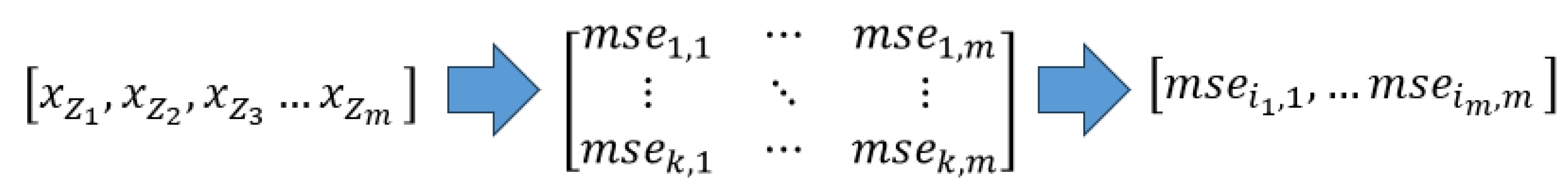
Figure 2.
Structure of Artificial Neural Networks.
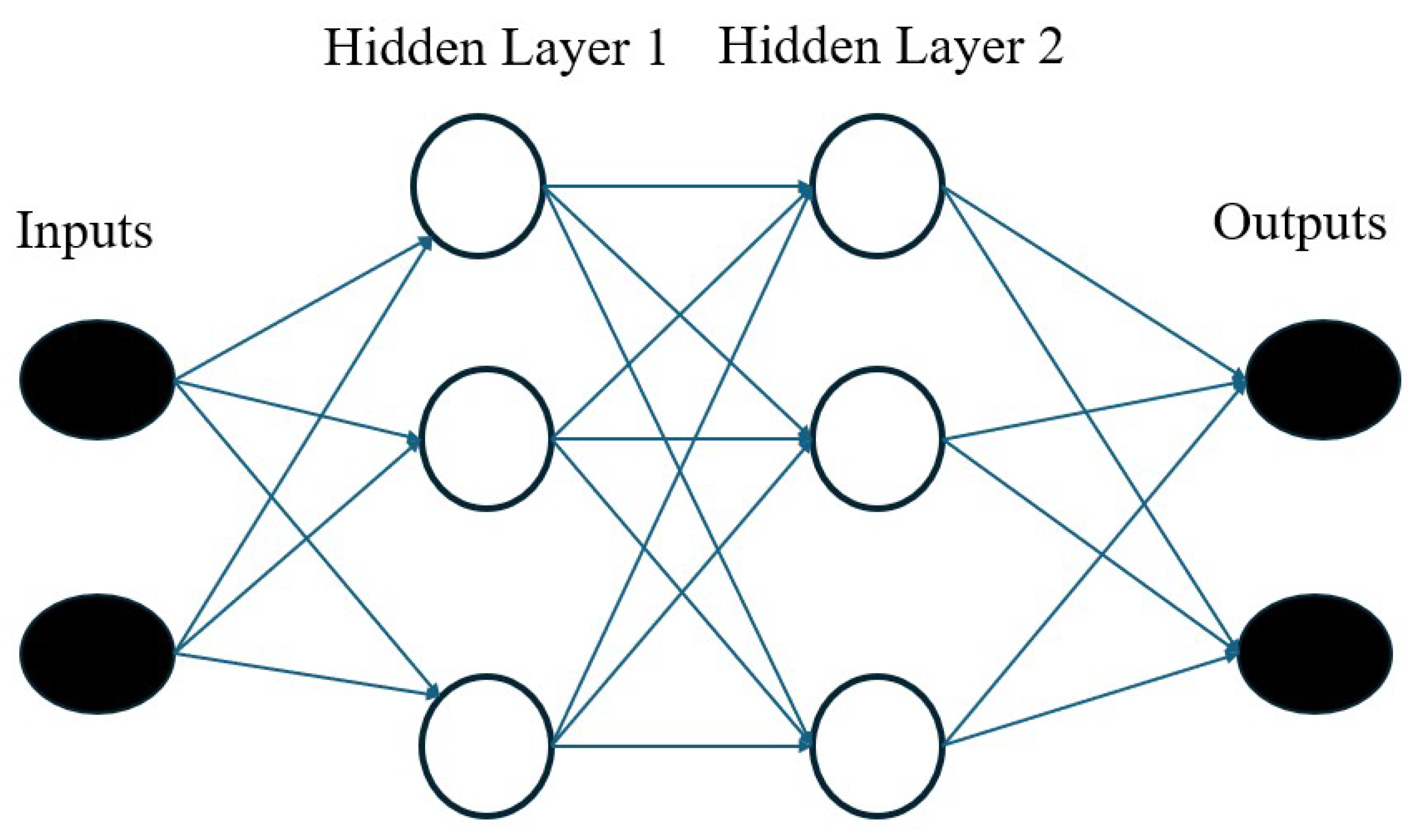
Figure 3.
Structure of a Random Forest.
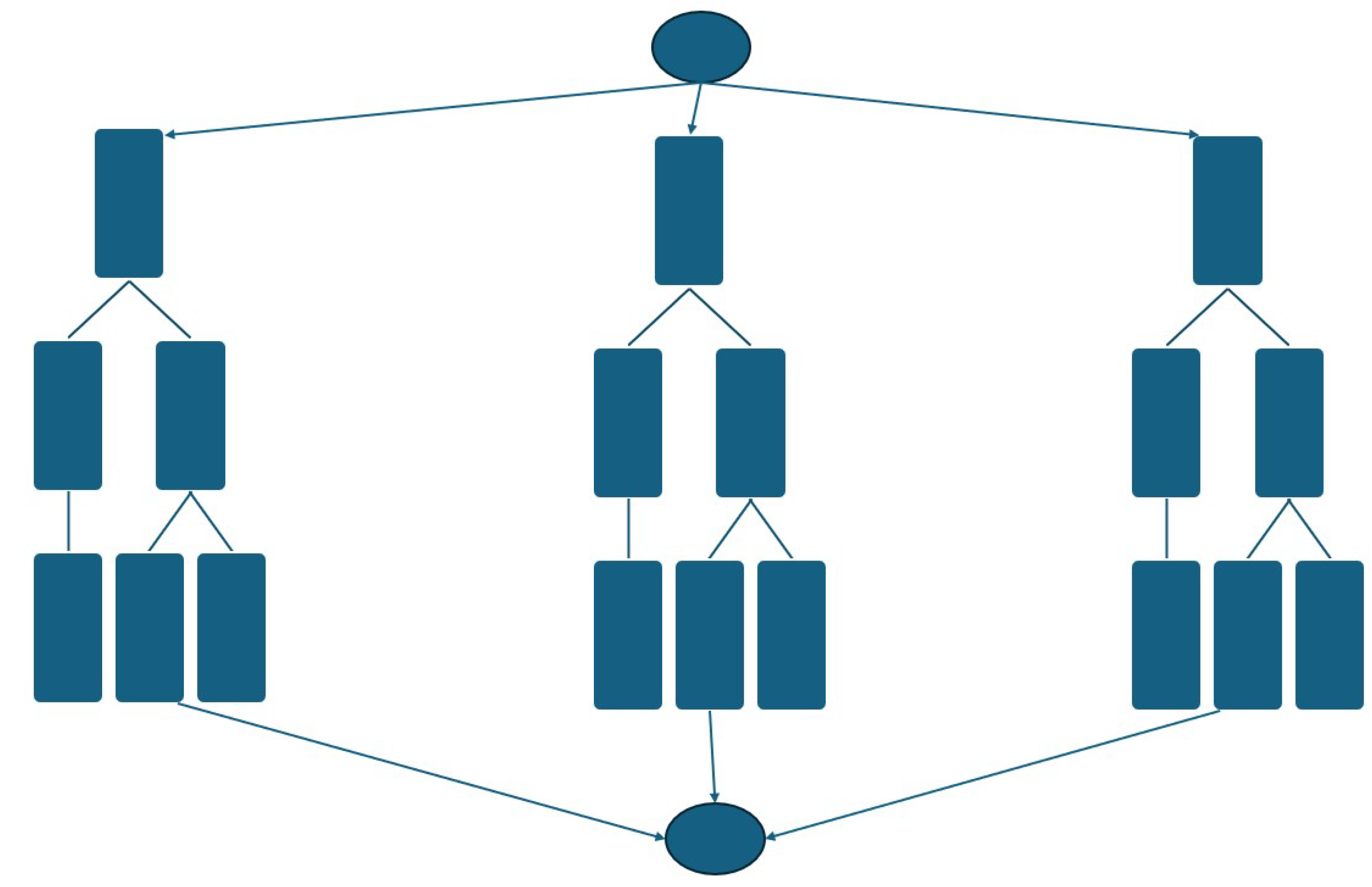
Figure 4.
Oil filter circuit.
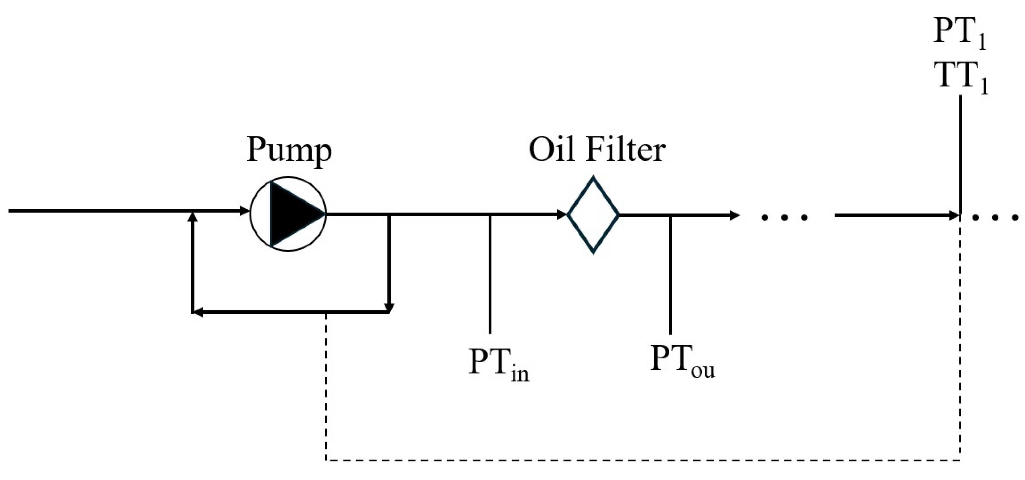
Figure 5.
Simulation of excessive filter clogging.
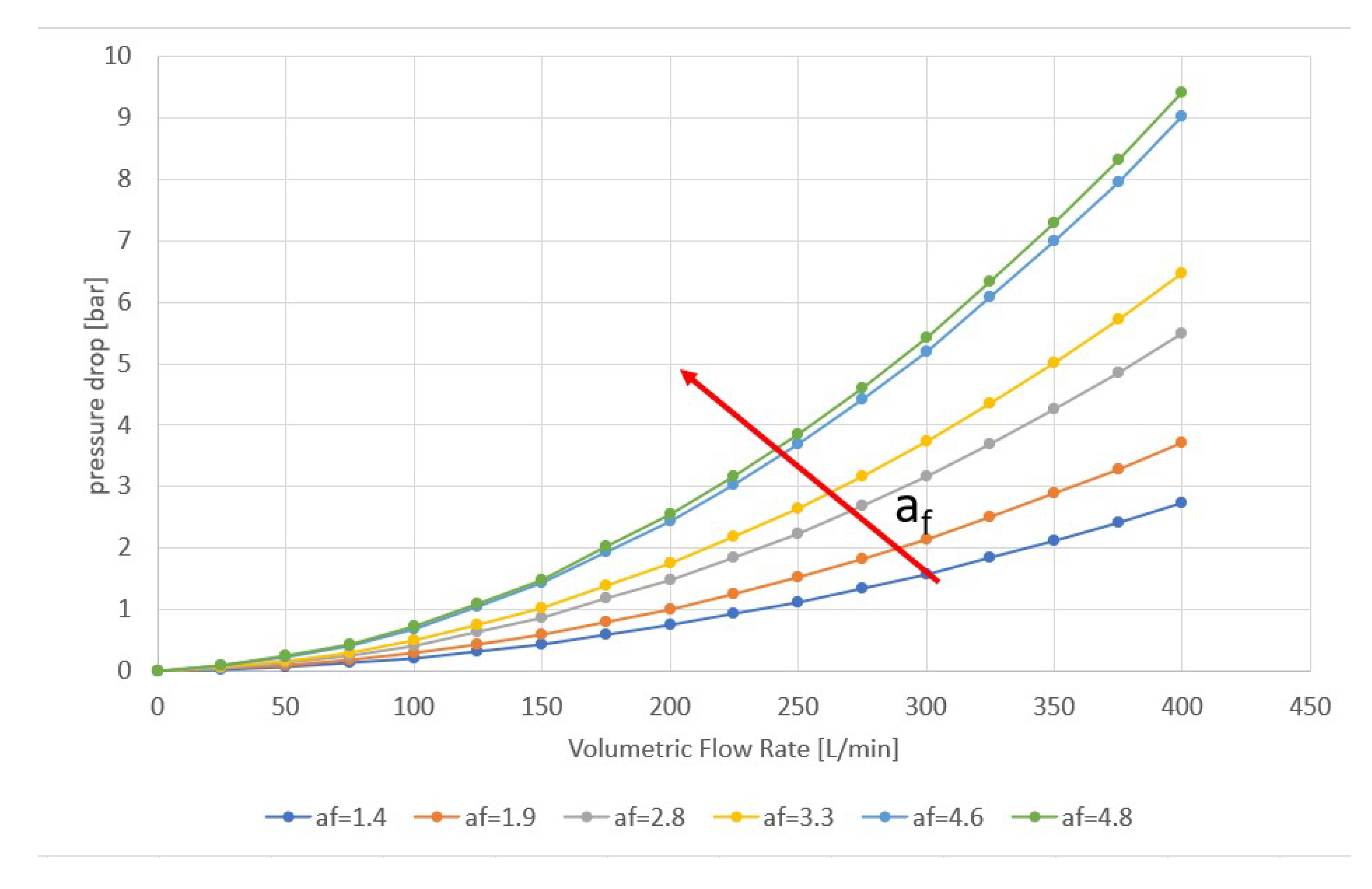
Figure 6.
Results by the Artificial Neural Network for .
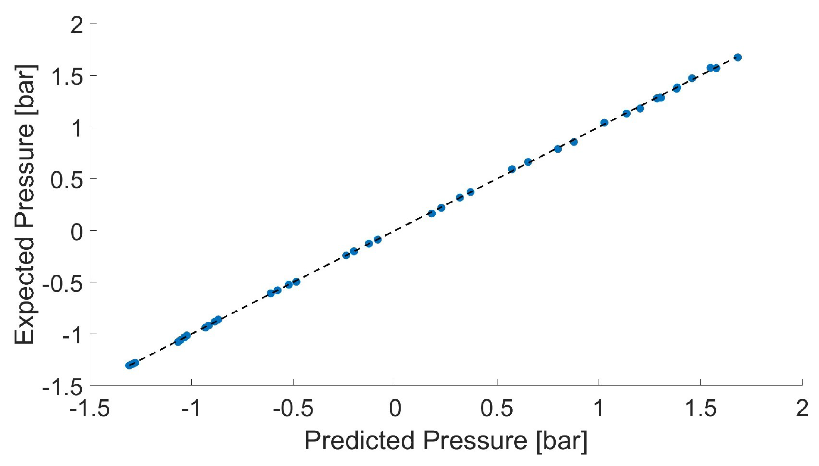
Figure 7.
Results by the Artificial Neural Network for .
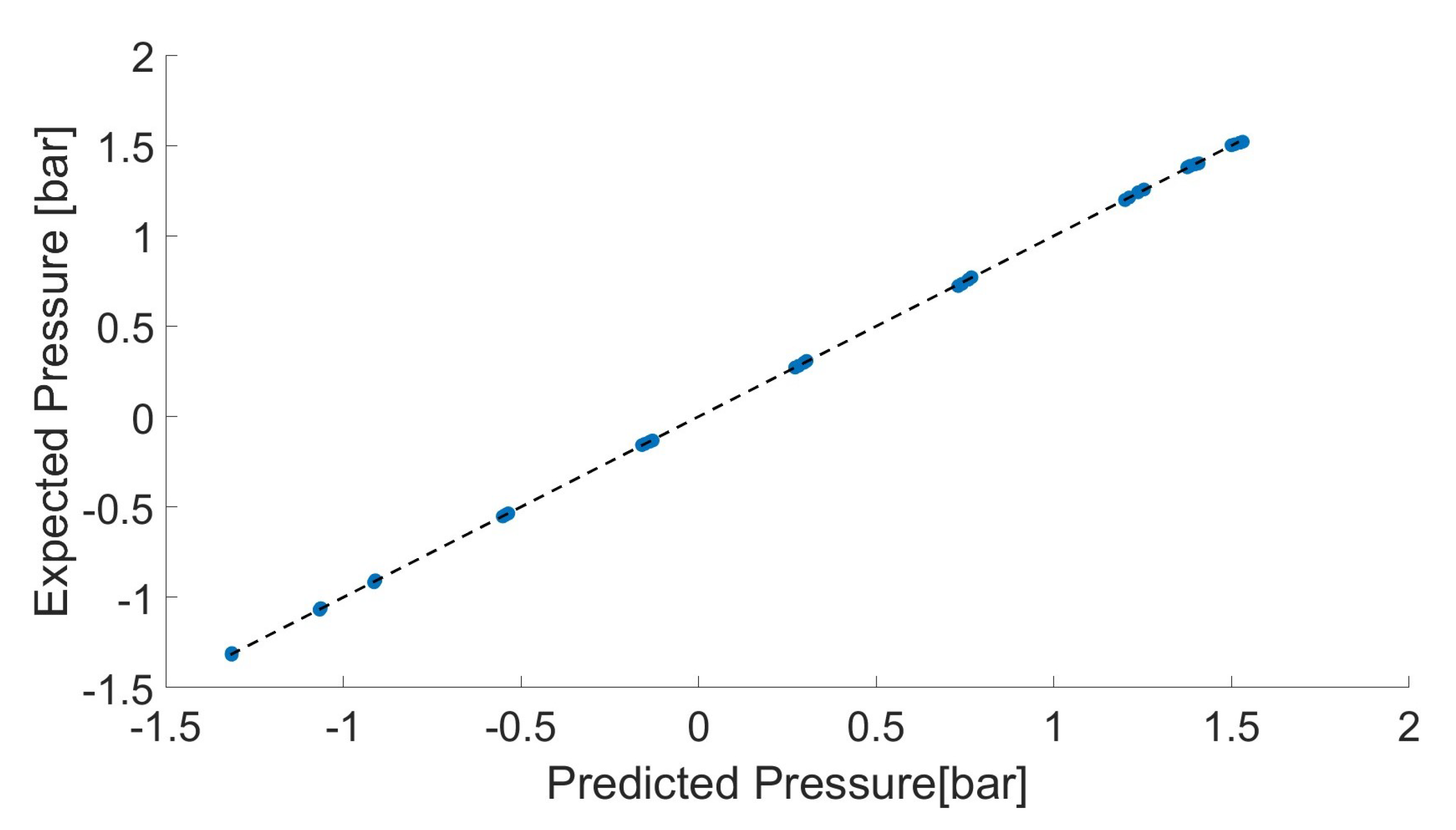
Figure 8.
Results by the Random Forest.
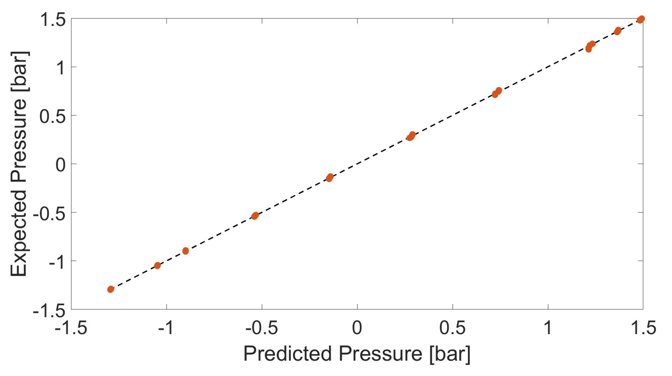
Figure 9.
Results by weighted ENN on input pressure sensor.
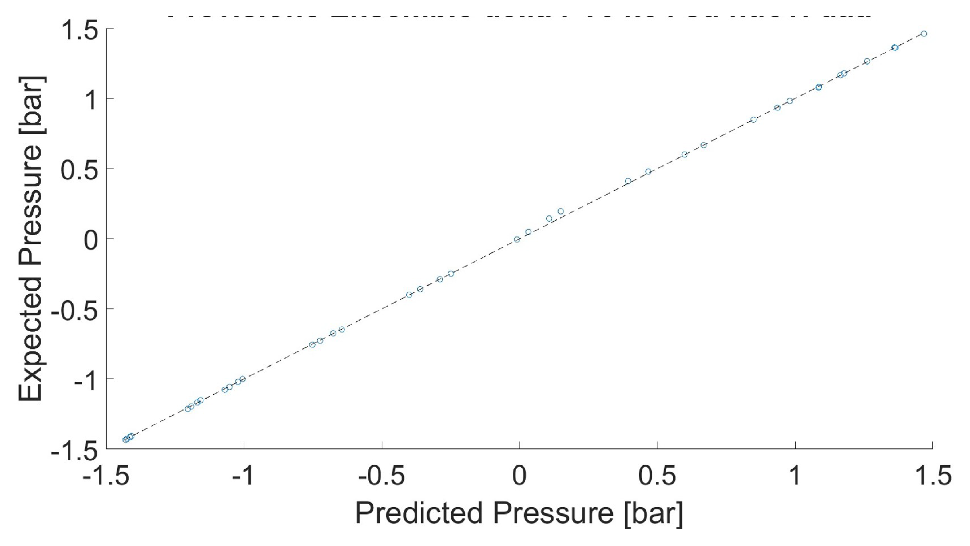

Table 1.
Specifications of the Artificial Neural Network
| Inputs | / and pump rotational speed |
| Outputs | Oil filter pressure drop |
| No. of hidden layers | 2 |
| No. of neurons | 24 (1st hidden layer) & 12 (2nd hidden layer) |
| Training algorithm | Levenberg-Marquardt |
Table 2.
Specifications of the Random Forest for
| Inputs | and pump rotational speed |
| Output | |
| Number of trees | 91 |
| MinLeafSize | 1 |
| MaxNumSplit | 92 |
Table 3.
Comparison between ANN and RF
| Performance | ANN | RF |
|---|---|---|
| MSE | () and () | |
| Computation time | 12 s | 105 s |
Table 4.
Specifications of the Ensemble Neural Networks
| Inputs | and pump rotational speed |
| Outputs | Oil filter pressure drop |
| No. of Neural Networks | 3 |
| Output Logic | arithmetic mean and weighted mean |
| Weight Value | 1.0 and 0.70 |
Table 5.
Results by the Ensemble Neural Networks
| Performance | Arith. mean ENN | Weight. mean ENN |
|---|---|---|
| MSE | ||
| Computation time | 46 s | 24 s |
Disclaimer/Publisher’s Note: The statements, opinions and data contained in all publications are solely those of the individual author(s) and contributor(s) and not of MDPI and/or the editor(s). MDPI and/or the editor(s) disclaim responsibility for any injury to people or property resulting from any ideas, methods, instructions or products referred to in the content. |
© 2024 by the authors. Licensee MDPI, Basel, Switzerland. This article is an open access article distributed under the terms and conditions of the Creative Commons Attribution (CC BY) license (http://creativecommons.org/licenses/by/4.0/).
Copyright: This open access article is published under a Creative Commons CC BY 4.0 license, which permit the free download, distribution, and reuse, provided that the author and preprint are cited in any reuse.


