Submitted:
20 June 2024
Posted:
21 June 2024
Read the latest preprint version here
Abstract
Orificed Hollow Cathodes are electric devices necessary for the functioning of common plasma thrusters for space applications. From their reliability mainly depends the success of a spacecraft’s mission equipped by electric propulsion. The development of plasma models is crucial in the evaluation of plasma properties within the cathodes that are difficult to measure due to the small dimensions. Many models, based on non-linear system of plasma equations, have been proposed in the open literature. These are solved commonly by means of iterative procedures. This paper investigates the possibility to solve them by means of Particle Swarm Optimization method. The results of the validation tests confirm the expected trends for all the unknowns; the confidence bound of the discharge current as function of mass flow rate is very narrow (2÷5V), moreover the results match very well the experimental data except at the lowest mass flow rate (0.08mg/s) and discharge current (1A), where the computations underpredict the discharge current to the utmost by 40%; the highest data dispersion regards the plasma density in the emitter region (± 20 % of the average value) and the wall temperatures (± 50K respect to the average values) of orifice and insert; those of the others variables are very tiny.
Keywords:
cathode
; plasma
; model
; PSO
1. Introduction
Orificed Hollow Cathodes (OHCs) [1] are used both as electronic source and/or neutralizer for Electric Propulsion (EP) devices e.g. Hall Effect Thrusters (HETs), Gridded Ion Thrusters (GITs), High Efficiency Multistage Plasma Thrusters (HEMPTs) [2]. A lot of computational tools, based on phenomenological models, also known as zero-dimensional (0D) or reduced-order models, aimed to predict OHCs’ plasma properties and performances and useful to support their design, have been developed since ’80s [3,4,5,6,7,8,9,10,11,12].
Also the Italian Aerospace Research Centre (CIRA) has developed its own design and analysis tools for Xenon fed OHCs (named PlasMCat) [13], that is based on Albertoni’s et al. model [6], whose plasma equations are corrected according to the suggestion by Wordingham et al. [14] and cathode’s internal pressure is computed by means of the empirical formula proposed by Taunay et al. [15]. Moreover a proper plasma model is included for the cathode-keeper gap.
The equations that constitutes the most of the models presented in the open literature [5,6,7,9,10,11,12] are commonly iteratively solved to face with their own non-linear characteristic. Each author adopts a different approach. PlasMCat follows a procedure similar to Albertoni et al. [6] and in agreement with them, has assessed that the adopted solution technique has limited stability because abrupt changes in geometry, flow rate or discharge current can cause the solution to diverge. This has given motivation to explore different solution strategies.
In this work the possibility to solve the whole system of models’ equations by means of a Particle Swarm Optimization (PSO) algorithm is investigated. PSO is a population based stochastic optimization technique developed by Dr. Eberhart and Dr. Kennedy in 1995 [16], inspired by social behaviour of bird flocking or fish schooling. PSO has been successfully applied in many research and application areas [17] and recently it has also been successfully used in EP application to solve the complex systems of non-linear equations used to model Helicon Plasma Thrusters’ (HPTs) plasma [18].
Hence, because of the relevant number of involved variables and to the associated strong non-linearity, in order to benefit from this approach, a code that searches for all the possible solutions of the plasma equations for OHCs has been built and tested.
The paper is organized as follows: the main definitions and the assumptions of the plasma model (whose equation are recalled in §Section 2.3 for completeness) are discussed in §Section 2; the optimization technique and its detailed model is presented in §Section 3; an application of the methodology is presented in §Section 4 where the results of the simulation are discussed; finally the conclusion are drawn in §Section 5.
2. Plasma Model of Hollow Cathode
2.1. Cathode Architecture
A sketch of a typical Orificed Hollow Cathode configuration is shown Fig. Figure 1. A neutral gas (e.g. Xenon, Argon, Krypton) flows in a conductive tube made of refractory metal (e.g. tantalum or molybdenum) or graphite. A low-work function material, namely insert, is placed inside the main tube. The electrons are extracted from the insert material by means of thermionic effect at a lower temperature with respect to the main tube. The most common insert materials are barium-based and rare-earth emitters (e.g. , ), which have respectively a work function of about 2 eV and 2.7 eV [1]. They provide a current densities as high as at a surface temperature of about 1300 K and 1900 K, respectively. The first type of emitters are highly susceptible to oxygen contamination while rare-earth based emitters react with many refractory metals at high temperatures (in this case a thin graphite sleeves is placed between the emitter and the main tube). An orifice plate is placed at the downstream end of the tube to increase the internal pressure. To warm up the insert to the emission temperature a heater is wrapped around the tube; thermal shields are usually added to reduce the radiation losses. The cathode tube and heater are surrounded by the keeper electrode, whose function is to help the extraction of the electrons to the discharge plasma and to protect the cathode from the ion bombardment.
2.2. Definition and Assumptions
The hollow cathode internal plasma volume is divided into three regions, the keeper region, pedix "k" (which includes the keeper orifice region and the cathode-keeper gap), the insert or emitting region, pedix "e", and the orifice region, pedix "o", as depicted in Fig. Figure 1. A set of conservation equations is written for each region (§Section 2.3) to compute averaged plasma properties (0-D model). The modelled plasma consists of neutrals, singly-charged ions and electrons. The unknown parameters are the electron temperatures (), the plasma densities (), the neutral densities (), the effective emission length (), the sheath potential (), the wall temperature of the emitter (), orifice () and keeper ().
- the heavy particles (ions and neutrals) are in a thermal equilibrium between each other and their temperature is assumed to be equal to the temperature of the wall, i.e. ;
- a chocked gas flow model is used in the orifice regions of both cathode tube and keeper;
- a double sheath potential drop is recorded at the orifice entrance region, thus a planar double sheath is modelled (Fig. Figure 1).
The neutral flow through the cathode’s insert, that is transitional, is not modelled as continuous and governed by the Poiseuille’s law, which is a well established assumption for 0D models [14]. Instead, the cathode internal pressure is computed by means of Taunay et al. formula [15].
For all the simulations described in this paper, Xenon is used as propellant because it is widely used in EP devices. Particularly, the electron-neutral cross section has been updated in order to include only elastic collisions as suggested by Wordingham et al. [14] and to take into account the most recent experimental data, a fit of which is proposed in Ref. [13].
2.3. Plasma Model Equations
The following subsections recall the equations presented in Ref. [13] and used to model the plasma in the three regions in which cathode’s internal volume has been divided.
Keeper
Orifice
The system of equations for the cathode’s orifice region writes a balance for the ion flux Eq.2(a) and for the power Eq.2(b), and states that pressure calculated by means of kinetic theory is equal to that computed with continuum flow and chocked orifice, Eq.2(c). The plasma number density (), the electron temperature (), and the density of the neutrals () in the orifice region are the unknowns.
Here the plasma resistance is calculated as:
The plasma resistivity is generally computed as:
and collision frequencies are:
where the Coulomb logarithm is:
and the fit for the Maxwellian Average elastic electron-neutral cross section () proposed in Ref. [13] for Xenon is:
| Values |
Insert
Four equations are written in order to get the unknown plasma number density (), electron temperature (), neutral density () and emitter sheath voltage drop () in the insert region. These are the balance for the ion flux, Eq.9(a), the current conservation, Eq.9(b) the power balance, Eq.9(c) and the continuity equations, Eq.9(d).
The plasma resistance in the insert region is computed as:
A voltage drop is supposed to be between insert and orifice region; the intensity of this double sheath is computed according to literature [5,6,9] by using the following expression:
The Xenon viscosity in is computed by means of the formula proposed by Goebel and Katz [1]:
True if . In the following, all the expressions for the current densities used in Eq.9 are recall for completeness:
3. Particle Swarm Optimization Methodology
3.1. Method’s Overview
The finding of a solution of a so complex system of equations would have had to be carried out by resorting to a very high number of manual attempts until the correct combination was reached. It was therefore decided to solve the equations system using a heuristic optimizer such as the Particle Swarm Optimization (PSO) [19,20,21].
PSO is a population based stochastic optimization technique developed by Dr. Eberhart and Dr. Kennedy in 1995[16], inspired by social behaviour of bird flocking or fish schooling. The particle swarm optimization concept consists in the generation of a swarm of individuals, each of them characterized by a proper set of variables’ value, and hence, a unique state variable vector, . During the generation of the swarm all these values are randomly assigned in such a way to cover the variables domain as it is defined in the initial problem setup. In fact, all the individuals try to find the problem’s solution searching inside the associated domain and their boundaries, using a performance index as main indicator. This latter is usually called fitness index or cost function. So, once the domain has been defined, it is necessary to determine the structure of the cost function to optimize. In this regard, the cost function can be written as a linear combination of target values and/or any constraints to be imposed. In this work it is required that all the residuals, as defined in the following, are minimized.
Now, deepening in the procedure, at the first iteration, after the swarm generation, the solver is applied to each individual in order to calculate the cost function that defines how much that solution would be good. The calculation of the cost function J is the starting point for the next iteration. In fact, to start the exploration of the variables’ domain, all the individuals need a proper velocity. This latter is calculated as the sum of many different contributions linked to their Personal Best and the Global Best index. The Personal Best (PB) and the Global Best (GB) are, respectively, the best solutions found from a single individual and from the whole swarm, in the exploration history. To understand what is best, each individual of the swarm need to remember the variables’ set associated at the best cost function encountered before. In this way, the information coming from the next iteration k+1 can be compared with the previous one, k, and the exploration process is driven towards the most promising region of the domain. Another contribution to the velocity calculation comes from the velocity itself at the previous iteration. In fact, this term is also called Inertia. With the same criterion, the term due to the PB is called Nostalgia, and the other one, due to the GB, is called Social. The composition of these three terms defines the new velocity for the next iteration k+1, as showed in Figure 2.
So, the Personal Best and the Global Best of that iteration are used to update the individual velocity and hence their position (variables’ set). These positions, in the respective domains, are the starting point for the next iteration. At each time step, the domain can be explored, iteration after iteration, changing the velocity of all the individuals and hence accelerating toward the updated Personal Best and Global Best. The cycle stops with the criteria selected by the user, at a fixed number of iterations, or in dynamic way depending from the number of concluded iterations without significant optimization. In both cases the user obtain the final solution that should also be the optimal one in that domain.
The theory behind the PSO, as for all the others heuristic techniques, excludes that the solution obtained could be effectively the optimal one in absolute sense [21]. This situation could be relevant when this technique is used in scientific field admitting high number of "local optimum" as for example in astrodynamics. Unfortunately, the OHC model seems to be very similar to this situation because of the high number of variables and equations and their strong non-linearity. So, it is reasonable to start the optimization process many times, to overcome, or at least mitigate, the possibility that the result was not the real best solution, in absolute sense. Also for this reason, in the last years, PSO has been updated with many variants and advancements [22,23,24,25] in order to enhance the research capability and/or faster convergence.
A schematic view of the entire cycle is reported in Fig. Figure 3.
3.2. PSO General Model
As aforementioned, the solution of the equation’s system has to be searched in a certain domain. The constrains are set to the ten independent variables i.e. neutral and plasma densities in the orifice and the emitter (), the electron and wall temperatures (), the emission length () and the plasma potential (). In fact, by analysing Eqs. 1, it is simple to verify that the keeper plasma unknowns () depend on the plasma density and the electron temperature of the orifice. Moreover the keeper wall temperature () is set constant to typical value. The ten parameters govern the entire problem and therefore represent the 10-dimensional exploration domain of the PSO method. The boundaries of the exploration domain (min and max) for each variable can be arbitrarily defined; clearly, reasonable values must be used to foster the research and do not waste computational effort in regions representing non-physical operative conditions. Thus, a good way to proceed is to use values in agreement with the typical value reported for cathodes, well characterized in open literature.
Once the domain has been defined it is necessary to initialize the swarm assigning an initial state and velocity for each individual. Between the ten variables defined above, some of those, such the electronic temperature , have a range with a minimum and maximum in the same order of magnitude, and the value of the specific variable can be assigned with a simply random approach. Other variables, instead, are defined in a range with an order of magnitude much greater than one, such as neutral density , that spans from up to . For this second kind of variables a different approach is required for the state generation. Using the notation of and , respectively, for the minimum and maximum of a general variable X of the state vector of the problem, the two different expressions can be considered:
with
and
with . Here is a random operator that randomly assumes values between 0 and 1.
The wider order of magnitude of certain variables is irrelevant for the initial velocity definition as it is quickly updated during the first iterations. Hence, in a simple manner, it is also defined the first velocity of each variable as follow:
At this point, after the swarm initialization, each individual, with its own state vector, represents a possible solution of the problem, hence it is processed in the numerical model, in order to solve the associated equations (plasma density, electronic temperature, etc...), and obtain the residuals of that specific running setup. So, the cost function J is evaluated, for each individual, as the sum of the residuals,
where:
where is the cost function evaluated for the individual at the iteration. Furthermore, all the residuals, as defined above, have been divided to their reference variable (i.e. Discharge Current, Power, and so on) in order to obtain dimensionless residuals with the same order of magnitude. This operation allows the optimization code to operate with different variables, but all with the same weight. Now, all these first cost functions are assigned as the PB of each individual, so:
while the GB has to be selected as the one with minimum value in the entire swarm, hence:
With this latter step, the swarm initialization can be said concluded, and the real optimization process can start. So, to update the state of all the individuals, using the information coming from the exploration, and hence from the swarm, the new velocities can be calculated with the ultimate form:
where i is the individual and k is the iteration, C1-C2-C3 are constants typically comprises between 0 and 2, X refers to the variable whose velocity is being calculated, and is a random operator that assume values between 0 and 1, as mentioned above.
Now, the individuals’ state can be updated with the velocity in order to start effectively the domain exploration:
This updated state is considered as a temporary state since it has to be checked respect to the original domain as defined at the beginning of this section. In fact, it could happen that the updated state results to be out of the domain bounds because of its movement due to the applied velocity. In this case, the state is corrected assigning the boundary value that it was trying to violate during the update.
With the updated state, also the cost function can be updated in order to compare the values with the ones calculated at the iteration before . If results to be minor than the iteration before, for one or more individuals, than its own Personal Best would be updated and so:
The same happens for the Global Best, where its own value is compared with all the PB of the entire swarm. If at least one individual have found a better solution , with respect to the GB of the iteration before , also the Global Best would be updated, so:
This criterion is the fundamental of this optimization technique, since it allow to drive the individuals close to the promising region of the domain where better solutions are found. From this point ahead the cycle is continuously repeated until the stop criterion is satisfied.
3.3. PSO Design and Rebuilding Approach
It has been assessed that the developed PSO-code base solver can be used both to support the preliminary design of new hollow cathodes and for the rebuilding of plasma properties, if the electrical characteristics are known.
To design a new cathode, primarily the cathode geometry (i.e. insert, orifice and keeper diameters, orifice and keeper-orifice lengths), the propellant mass flow rate, the insert material and the current value have to be set. Secondly, a reasonable exploration domain must be defined. Then PSO-code can be run. It will give the evaluation of all the unknowns within a confidence bounds.
It has been verified (this will be clear in the application example of §Section 4), that the trend of emitter wall temperature as function of mass flow rate, can be better reproduced by setting a target total discharge voltage,, calculated as the ratio of the absorbed power on the discharge current .
Thus it’s necessary to modify the formulation of the cost function J since it has to consider a new parameter, i.e. , as in Eq. 29. In fact, in this case, the optimization process have to minimize also the difference between the total voltage and the target value .
It is clear that this last approach can be used also for the rebuilding of plasma properties in an existing Hollow Cathode when the experimental electrical characteristics are known.
4. Results
This section reports the results of an application of the described methodology. The boundaries of the PSO exploration domain (Table 1) for each variable have been defined in agreement with the values estimated for the AlphCA Cathode, that is an OHC developed and tested by SITAEL [26,27]. A keeper surface temperature of 800K has been set for all the calculations according to the experimental measurements.
AlphCA is composed by a Tantalum tube 7.5 mm in diameter, with a polycrystalline LaB6 insert 3 mm in internal diameter and 6 mm in length. The thickness and the length of the tube are approximately equal to 0.3 mm and 20.6 mm, respectively. The orifice has a diameter of 0.4 mm and a length of 0.36 mm. The Molybdenum-alloy keeper presents a 0.6 mm diameter orifice, whereas the cathode-to-keeper gap is 2 mm in the longitudinal direction. Because the length of keeper orifice has not been found, a realistic value of 0.3 mm has been selected to perform the calculation. The propellant is pure Xenon (contamination issues are not considered in the model). The cathode operates at a discharge current ranging from 1 to 3 A and at mass flow rates between 0.08 and 1 mg/s. The electrical characteristics in this operational envelope, measured in diode mode with keeper [27], are reported in Fig. Figure 4, as test2 and test3.
The shaded zone in Fig. Figure 4 represents the confidence bound of the total discharge voltage, limited by the curves, in which the PSO solutions lay. More in detail, the mean , and the variance , have been calculated for the best ten solutions obtained at each mass flow rate value. The mean and the variance are calculated with the standard equation, respectively as follow:
Hence, the standard deviation is used to generate the confidence bound () around the mean values.
Several considerations arise from the observation of Figure 4:
- the confidence bounds range between 2V and 5V for the current span examined;
- the discharge current initially decreases with the mass flow rate, as expected, but it increases at the highest mass flow rates; this could be attributed to the absence of a second double sheath at the cathode orifice exit that could be negative because the plasma density decreases passing from the orifice region to the keeper region (see Fig. Figure 7a, Figure 8a);
- the shaded zone perfectly cover the experimental measurements obtained for a discharge current of 2A and it is slightly higher at 3A; at 1A and at lowest mass flow rates, the discharge current is 40% lower, at its maximum, than the reference data, probably because the system of equation does not adequately describes the plasma physics in those conditions.
Figure 4.
Confidence bound of the total discharge voltage as function of the propellant mass flow rate computed at 1A (a), 2A (b), 3A (c) by means of PSO; experimental measurements from Ref. [27] are reported for comparison.
Figure 4.
Confidence bound of the total discharge voltage as function of the propellant mass flow rate computed at 1A (a), 2A (b), 3A (c) by means of PSO; experimental measurements from Ref. [27] are reported for comparison.
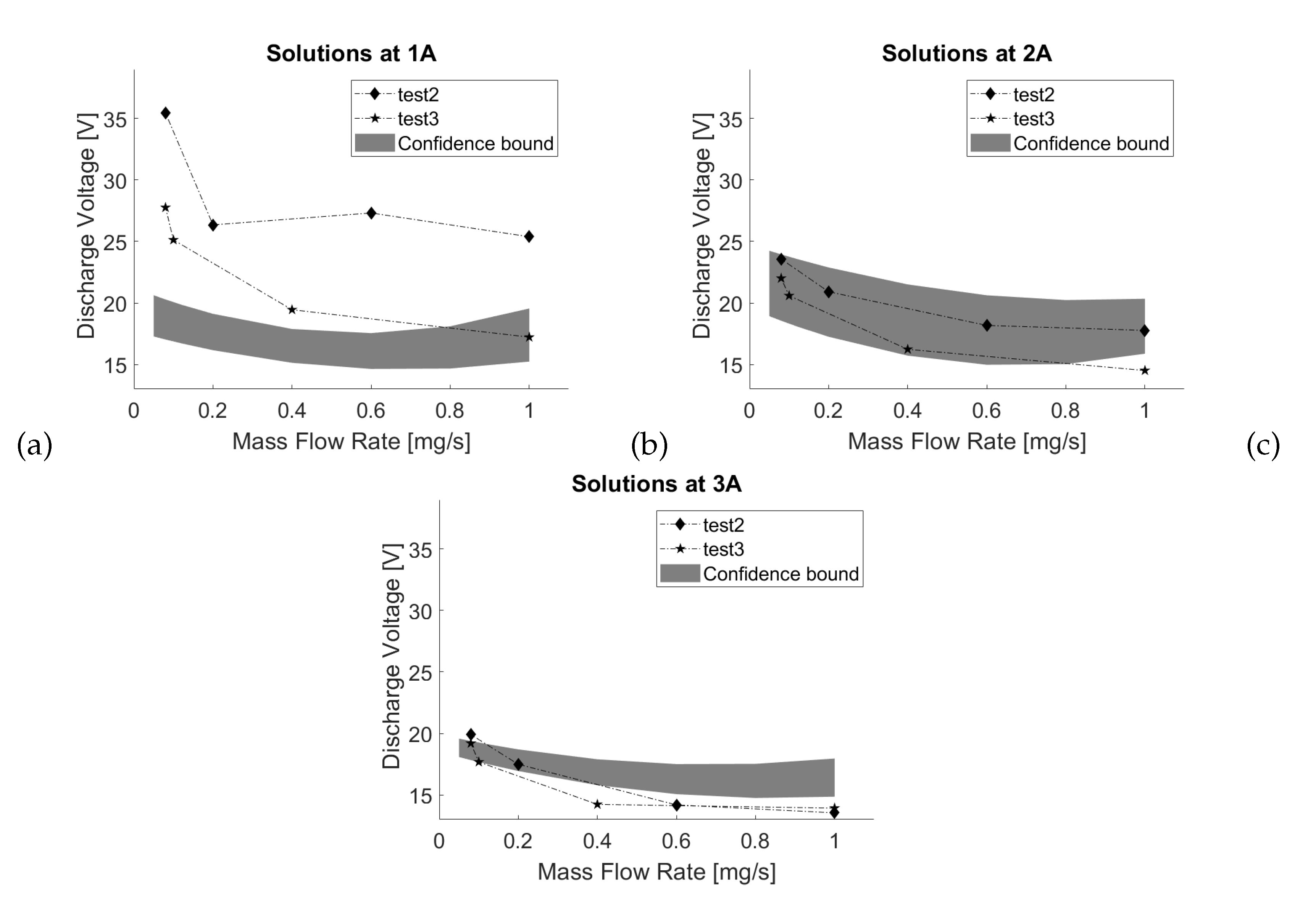
Figure 5.
Residual’s mean value, evaluated for the ten solutions at 2A.
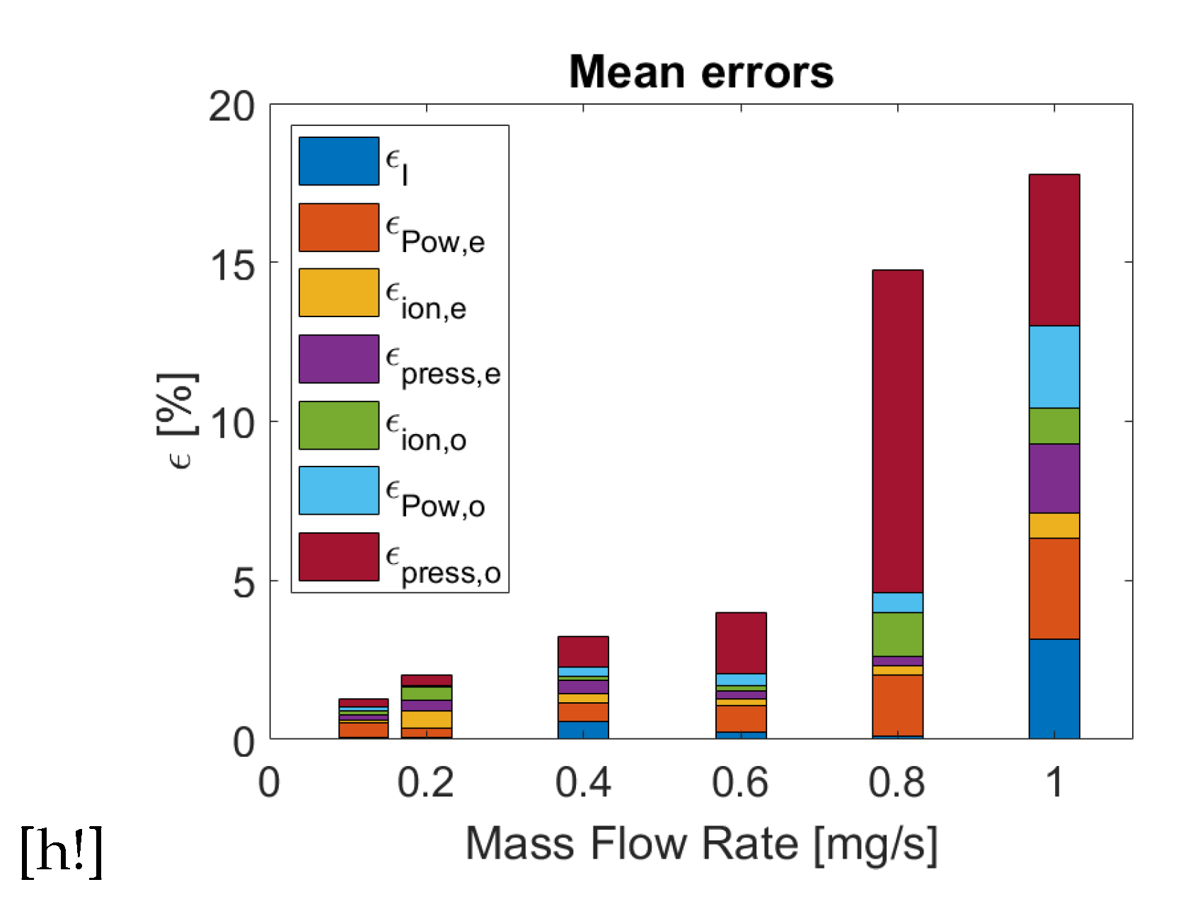
Figure 6.
(a) Plasma density; (b) Neutral density; (c) Electronic Temperature; (d) Emitter Temperature as function of mass flow rate. All the figures refer to physical properties evaluated in the emitter region, in case of operative points at 1A and 2A.
Figure 6.
(a) Plasma density; (b) Neutral density; (c) Electronic Temperature; (d) Emitter Temperature as function of mass flow rate. All the figures refer to physical properties evaluated in the emitter region, in case of operative points at 1A and 2A.
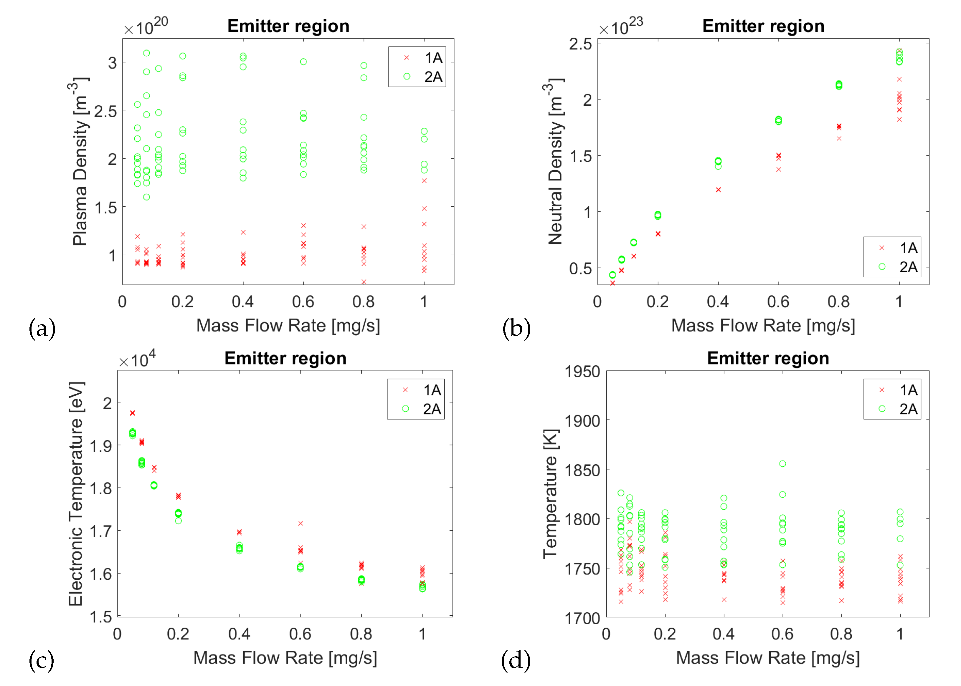
Figure 7.
(a) Plasma density; (b) Neutral density; (c) Electronic Temperature; (d) Emitter Temperature as function of mass flow rate. All the figures refer to physical properties evaluated in the orifice region, in case of operative points at 1A and 2A.
Figure 7.
(a) Plasma density; (b) Neutral density; (c) Electronic Temperature; (d) Emitter Temperature as function of mass flow rate. All the figures refer to physical properties evaluated in the orifice region, in case of operative points at 1A and 2A.
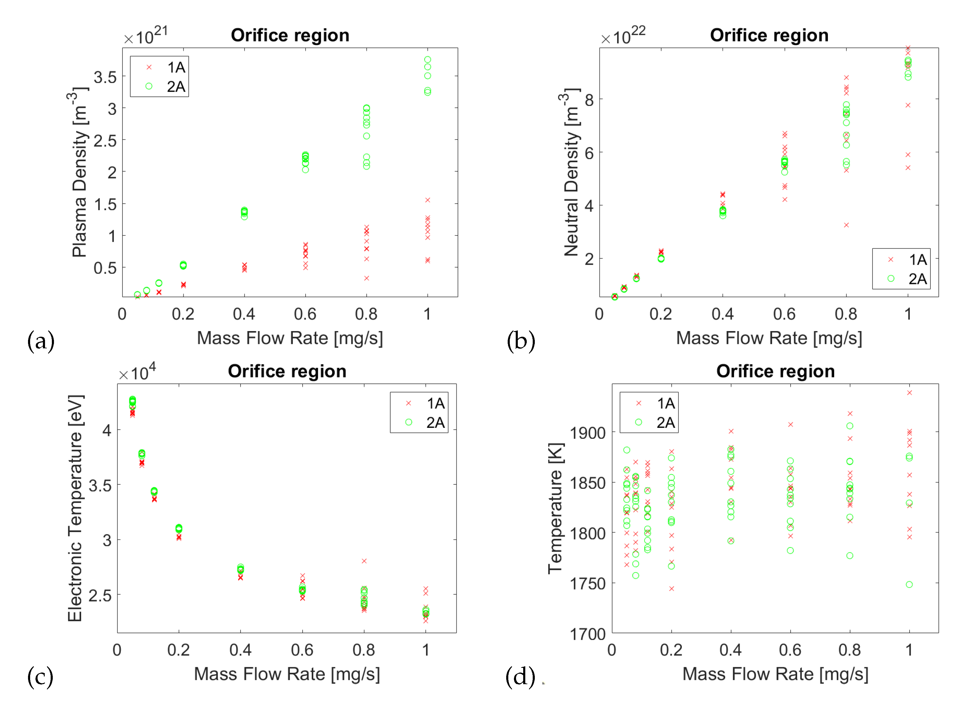
Figure 8.
(a) Plasma density; (b) Neutral density; (c) Electronic Temperature as function of mass flow rate. All the figures refer to physical properties evaluated in the keeper region, in case of operative points at 1A and 2A.
Figure 8.
(a) Plasma density; (b) Neutral density; (c) Electronic Temperature as function of mass flow rate. All the figures refer to physical properties evaluated in the keeper region, in case of operative points at 1A and 2A.

Figure 6, Figure 7, Figure 8 report the best ten solutions obtained for the operative point at 1A and 2A in the whole mass flow rate span. These ten solutions have been selected from the PSO algorithm looking at the cost function. In fact, the cost function J is defined as the sum of the residuals evaluated for each equation, as reported in §Section 3.2. Thus, with this assumption, the value of J can be used as a direct and global index of the solution quality.
Figure 5 presents the errors, , evaluated as the mean value of the ten solutions at 2A, respect to the mass flow rates as example (similar figure would be drawn at 1A). The ten solutions presented at 1A and 2A, Fig. Figure 6- Figure 8, are characterised by a J value that typically remains under the 5% from the minimum mass flow rate up to 0.6mg/s. Beyond this value, and up to 1mg/s, the residuals, , tend to increase as obviously do the cost function J, in consequence. This circumstance is also put in evidence from the greater dispersion of the solutions while moving toward the higher mass flow rate values. Anyway, also in this region of greater uncertainties, the J values are limited to 20% and 40%, respectively for the cases at 2A and 1A. Moreover, also in the worst case, the mean value of a single residual is no greater than 10% as in Fig. Figure 5, where the greater error is due to the calculation of the pressure in the orifice region.
All the trends of plasma properties ( Fig. Figure 6, Figure 7 and Figure 8) reflect those reported in the open literature [5,6]: the electron temperatures decreases with the mass flow rate; the neutral densities increases as well as the plasma densities. The orifice temperature slightly increases whereas no particular trend can be desumed for the emitter temperature.
The Electron Temperatures (Fig.Figure 6c, Figure 7c, Figure 8c) , the plasma (Fig.Figure 6a, Figure 7a, Figure 8a) and neutral (Fig.Figure 6b, Figure 7b, Figure 8b) densities found by PSO are very close to each other, generating a confidence region that seems to be very tight. The higher dispersion is that of emitter plasma density (i.e. ± 20 % of the average value). The wall temperatures of the emitter and orifice lay within less than 100K bound. Nevertheless it must be remarked that the PSO has been able to get the order of magnitude of neutral and plasma densities by searching within a range of three order of magnitudes!
Figure 9 shows the PSO targeting the experimental measurements [27] of the discharge voltage as function of mass flow rate at 2A (i.e. PSO using Eq. 29). It has been found that the results perfectly match the results get without the assumption made with Eq.29 (for this reason they are not shown). The only difference regards the emitter wall temperature. Figure 10 highlights that with this approach the expected increasing trend of the temperature can be detected. Moreover, the confidence bound is narrower.
Computational Effort
The optimization code developed in this framework, namely the PSO, has been written in Matlab environment. Simulations are conducted on a Personal Computer Intel-i7 @ 1.80GHz with 16.0GB RAM. For each research and optimization cycle an amount of 20mln possible solutions are evaluated in less than 7 minutes from which are extracted the best ten solutions. More in detail, a swarm of 2000 individuals for 1000 iterations has been used, for 10 cycles. As aforementioned, the powerful of this method lays in the capability to be very fast and completely independent from the initial condition. In fact, this independence allow to completely overcome the initial condition estimation problem, as reported in the open literature [6]. Anyway, faster or slower convergence can be selected changing the coefficients C1,C2 and C3 in the velocity equation (Eq. 25) to balance the exploration and convergence dominance.
5. Conclusions
The paper has investigated the feasibility of using the Particle Swarm Optimization technique to solve a non-linear system of equations describing the plasma physics within Orificed Hollow Cathodes.
The results of the assessment test cases, conducted on Sitael AlphCA, have shown that the coupling between PSO and plasma model reveals itself as fast, powerful and accurate preliminary design and rebuilding tool for OHCs.
The trends of all the unknowns of the problem are well predicted. Particularly, the discharge current as function of mass flow rate is predicted with a confidence bound in the range 2 ÷ 5V for the current span examined. The computations at 2A and 3A well match the experimental data whereas at 1A and low mass flow rates, the discharge current is underestimated (maximum by 40%), probably because the system of equation is inadequate to describe the plasma physics in those conditions. The discharge current trend as function of mass flow rate is of a parabolic type for all current: it initially decreases, as expected, but it increases at high mass flow rates. This could be due to the absence in the model of a double sheath at the cathode orifice exit that could damp the discharge voltage which increases at high mass flow rate.
All the others unknowns of the problem are computed with a very tiny confidence bound with the exception of the plasma density in the emitter region (± 20 % of the average value) and the wall temperature of the emitter and the orifice (± 50K respect to the average values). Regarding plasma densities, it is worth to remark that the PSO has been able to get within a range of three order of magnitude the right one for neutral and plasma densities.
It has been verified that the confidence bound of the emitter temperature can be reduced and its trend can be improved by targeting the discharge voltage.
The difficulty to find solutions of the complex system of equation characterizing the plasma within the OHC has been fully overcame with the usage of the PSO technique. This enables the possibility to easily perform sensitivity studies on all the geometrical parameters of the cathode model, as well as quickly testing model modifications (i.e. the addiction of the aforementioned double sheath at the cathode orifice exit ).
Short Biography of Authors
 Coppola Giovanni holds a Master degree in Space and Astronautical Engineering at the italian University of Rome, La Sapienza. He works in CIRA (Italian Aerospace Research Center), at the Space Division as researcher of the Space Propulsion Laboratory. He worked as researcher and system engineer in international projects related to hyper-sonic vehicles and electric propulsion systems. He is mainly involved in the CIRA electric propulsion laboratory projects and activity as researcher. The recent activities are associated with the development of numerical tools for the preliminary design of Gridded Ion Thrusters (GITs), Helicon Plasma Thrusters (HPTs) and HEMPT. Other activities are related to plasma modelling and optimization techniques.
 Mario Panelli holds a PhD in Aerospace Naval and Quality Management Engineering from the University of Naples, Federico II. He currently works in CIRA (Italian Aerospace Research Center), being affiliated to the Propulsion and Exploration Division as researcher of the Space Propulsion Laboratory. He worked as researcher, project and system engineer in different national and international project in the topics of methane-based propulsion systems, hybrid propulsion, solid propulsion and electric propulsion. He is involved in the CIRA electric propulsion projects as project engineer and researcher. His most recent activities are associated with design and testing of Orifice Hollow Cathodes (OHCs) and Hall Effect Thrusters (HETs), plasma and erosion modelling, and preliminary design of Gridded Ion Thrusters (GITs), Helicon Plasma Thrusters (HPTs) and HEMPT.
 Francesco Battista holds a PhD in Aerospace Engineering from University of Pisa. He currently works in CIRA (Italian Aerospace Research Center), being affiliated to the Propulsion and Exploration Division as responsible of the Space Propulsion Laboratory. He worked as system engineer and project manager in different national and international project mainly in the topics of methane-based propulsion systems, hybrid propulsion and electric propulsion. He is involved in the CIRA electric propulsion projects as project manager and technical responsible. He is author or co-author of more than 100 papers, published on international journals and conference proceedings.
Author Contributions
Conceptualization M.P.; methodology, G.C. and M.P.; software, G.C.; validation, G.C.; formal analysis, G.C.; data curation, M.P. and G.C.; writing—original draft preparation, G.C. nd M.P.; writing—review and editing, F.B.; visualization, G.C.; supervision, F.B. and M.P.; project administration, F.B. All authors have read and agreed to the published version of the manuscript.
Funding
This research was funded by the Italian research program in aerospace, PRORA DM662/20 (Programma Operativo Ricerche Aerospaziali) entrusted by MIUR (Ministero dell’Istruzione , Ministero dell’Università e della Ricerca).
Institutional Review Board Statement
Not applicable.
Informed Consent Statement
Not applicable.
Data Availability Statement
The data presented in this study are available on request from the corresponding author.
Acknowledgments
The authors would like to thank all the space propulsion laboratory guys for the stimulating research environment.
Conflicts of Interest
The authors declare no conflict of interest.
Abbreviations
The following abbreviations are used in this manuscript:
| OHCs | Orifice Hollow Cathodes |
| EP | Electric Propulsion |
| HETs | Hall Effect Thrusters |
| GITs | Gridded Ion Thrusters |
| HEMPTs | High Efficiency Multistage Plasma Thrusters |
| PSO | Particle Swarm Optimization |
| HPTs | Helicon Plasma Thrusters |
| CIRA | Italian Aerospace Research Centre |
| PlasMCat | Plasma Model for Cathodes |
| RHS | Right Hand Side |
| LHS | Left Hand Side |
| PB | Personal Best |
| GB | Global Best |
Symbols
| A | = Area |
| L | = Length |
| r | = Radius |
| d | = Diameter |
| q | = Elementary charge |
| = Boltzmann’s constant | |
| = Vacuum permittivity | |
| = Residual | |
| = Electric field at the cathode sheath | |
| = Discharge current | |
| j | = Current density |
| = Ionization rate coefficient | |
| = Electron mass | |
| = Ion mass | |
| = Mass flow rate | |
| n | = Density |
| = Ion rate | |
| p | = Pressure |
| P | = Power |
| R | = Resistance |
| T | = Temperature |
| V | = Potential |
| = Work function | |
| = Degree of ionization | |
| = Plasma resistivity | |
| = Collision frequency | |
| = Cross section, standard deviation | |
| = Specific heat ratio | |
| M | = Molecular Weight |
| = viscosity | |
| = Coulomb Logarithm | |
| D | = material-specific Richardson-Dushman constant |
| = Average ionization energy (12.12 eV for Xenon) | |
| Subscripts | |
| n | = neutral |
| p | = plasma |
| e | = emitter, electron |
| o | = orifice |
| k | = keeper |
| = electron-neutral | |
| = electron-ion | |
| i | = ion moving at Bohm speed |
| = ion or ionization | |
| = electron recombination | |
| = thermionic emission | |
| = thermal | |
| = effective | |
| s | = emitter surface |
| w | = wall |
| = double sheath |
References
- Goebel, D.M.; Katz, I. Fundamentals of electric propulsion: ion and Hall thrusters; Vol. 1, John Wiley & Sons, 2008.
- Lev, D.R.; Mikellides, I.G.; Pedrini, D.; Goebel, D.M.; Jorns, B.A.; McDonald, M.S. Recent progress in research and development of hollow cathodes for electric propulsion. Reviews of Modern Plasma Physics 2019, 3, 6. [Google Scholar] [CrossRef]
- Siegfried, D.; Wilbur, P. An investigation of mercury hollow cathode phenomena. 13th International Electric Propulsion Conference, 1978, [https://arc.aiaa.org/doi/pdf/10.2514/6.1978-705]. [CrossRef]
- Salhi, A. Theoretical and experimental studies of orificed, hollow cathode operation. PhD thesis, Ohio State University, 1993.
- Domonkos, M.T. Evaluation of low current orificed hollow cathode. PhD thesis, Michigan University, 1999.
- Albertoni, R.; Pedrini, D.; Paganucci, F.; Andrenucci, M. A Reduced-Order Model for Thermionic Hollow Cathodes. IEEE Transactions on Plasma Science 2013, 41, 1731–1745. [Google Scholar] [CrossRef]
- Korkmaz, O., Global numerical model for the evaluation of the geometry and operation condition effects on hollow cathode insert and orfice region plasmas. In MSc dissertation, Bogazici University; 2015.
- Taunay, P.Y.C.; Wordingham, C.J.; Choueiri, E. A 0-D model for orificed hollow cathodes with application to the scaling of total pressure. AIAA Propulsion and Energy, Indianapolis, IN, 2019.
- Gurciullo, A.; Fabris, A.L.; Potterton, T. Numerical study of a hollow cathode neutraliser by means of a zero-dimensional plasma model. Acta Astronautica 2020, 174, 219–235. [Google Scholar] [CrossRef]
- Gondol, N.; Tajmar, M. A volume-averaged plasma model for heaterless C12A7 electride hollow cathodes. CEAS Space Journal 2023, 15, 431–450. [Google Scholar] [CrossRef]
- Potrivitu, G.C.; Laterza, M.; Ridzuan, M.H.A.B.; Gui, S.Y.C.; Chaudhary, A.; Lim, J.W.M. Zero-Dimensional Plasma Model for Open-end Emitter Thermionic Hollow Cathodes with Integrated Thermal Model. Proceedings of 37th International Electric Propulsion Conference Massachusetts Institute of Technology, Cambridge, MA, USA, 2022, Vol. IEPC-2022-116.
- Potrivitu, G.C.; Xu, S. Phenomenological plasma model for open-end emitter with orificed keeper hollow cathodes. Acta Astronautica 2022, 191, 293–316. [Google Scholar] [CrossRef]
- Panelli, M.; Giaquinto, C.; Smoraldi, A.; Battista, F. A Plasma Model for Orificed Hollow Cathode. 36th International Electric Propulsion Conference, Wien, Austria, 2019, Vol. IEPC-2019-452.
- Wordingham, C.J.; Taunay, P.Y.C.R.; Choueiri, E.Y. Critical Review of Orficed Hollow Cathode Modeling. 53rd AIAA/SAE/ASEE Joint Propulsion Conference, Atlanta, GA, 2017.
- Taunay, P.Y.C.; Wordingham, C.J.; Choueiri, E., An empirical scaling relationship for the total pressure in hollow cathodes. In 2018 Joint Propulsion Conference; [https://arc.aiaa.org/doi/pdf/10.2514/6.2018-4428]. [CrossRef]
- Kennedy, J.; Eberhart, R. Particle swarm optimization. Proceedings of ICNN’95 - International Conference on Neural Networks, 1995, Vol. 4, pp. 1942–1948 vol.4. [CrossRef]
- Kulkarni, M.N.K.; Patekar, M.S.; Bhoskar, M.T.; Kulkarni, M.O.; Kakandikar, G.; Nandedkar, V. Particle swarm optimization applications to mechanical engineering-A review. Materials Today: Proceedings 2015, 2, 2631–2639. [Google Scholar] [CrossRef]
- Coppola, G.; Panelli, M.; Battista, F. Preliminary design of helicon plasma thruster by means of particle swarm optimization. AIP Advances 2023, 13, 055209. [Google Scholar] [CrossRef]
- Zhang, Y.; Wang, S.; Ji, G.; others. A comprehensive survey on particle swarm optimization algorithm and its applications. Mathematical problems in engineering 2015, 2015. [Google Scholar] [CrossRef]
- Houssein, E.H.; Gad, A.G.; Hussain, K.; Suganthan, P.N. Major advances in particle swarm optimization: theory, analysis, and application. Swarm and Evolutionary Computation 2021, 63, 100868. [Google Scholar] [CrossRef]
- Bai, Q. Analysis of particle swarm optimization algorithm. Computer and information science 2010, 3, 180. [Google Scholar] [CrossRef]
- Jain, M.; Saihjpal, V.; Singh, N.; Singh, S.B. An overview of variants and advancements of PSO algorithm. Applied Sciences 2022, 12, 8392. [Google Scholar] [CrossRef]
- Kulkarni, M.N.K.; Patekar, M.S.; Bhoskar, M.T.; Kulkarni, M.O.; Kakandikar, G.; Nandedkar, V. Particle swarm optimization applications to mechanical engineering-A review. Materials Today: Proceedings 2015, 2, 2631–2639. [Google Scholar] [CrossRef]
- Ramírez-Ochoa, D.D.; Pérez-Domínguez, L.A.; Martínez-Gómez, E.A.; Luviano-Cruz, D. PSO, a swarm intelligence-based evolutionary algorithm as a decision-making strategy: A review. Symmetry 2022, 14, 455. [Google Scholar] [CrossRef]
- Moazen, H.; Molaei, S.; Farzinvash, L.; Sabaei, M. PSO-ELPM: PSO with elite learning, enhanced parameter updating, and exponential mutation operator. Information Sciences 2023, 628, 70–91. [Google Scholar] [CrossRef]
- Ducci, C., O.S.D.D.A.R.; Andrenucci, M. HT100D performance evaluation and endurance test results. Proceedings of 33rd Int. Electric Prop. Conf., IEPC2013, Washington, D.C., 6-10, Oct., 2013, Vol. IEPC-2013-140.
- Albertoni, R., P.D.P.F.; Andrenucci, M. Experimental Characterization of a LaB 6 Hollow Cathode for Low-Power Hall Effect Thrusters. Proceedings of Space Propulsion Conference, SPC2014, Cologne, Germany, 19-22, May, 2014.
- Meeker, D., inite Element Method Magnetics–Version 4.0 User’s Manual; 2006.
Figure 1.
(a) Schematic of typical Orifice Hollow Cathode and (b) sketch of plasma model regions.
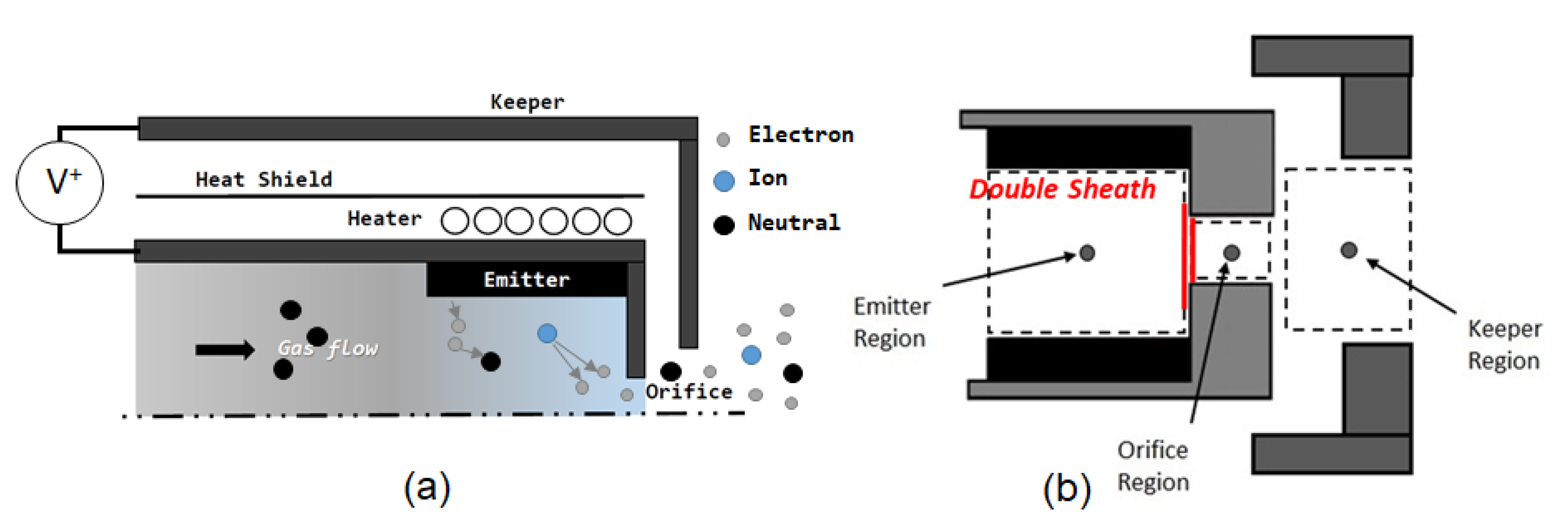
Figure 2.
PSO:Schematic view of the velocity contributions.
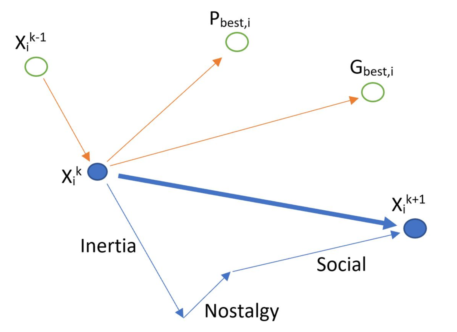
Figure 3.
Schematic view of the PSO algorithm developed for OHCs.
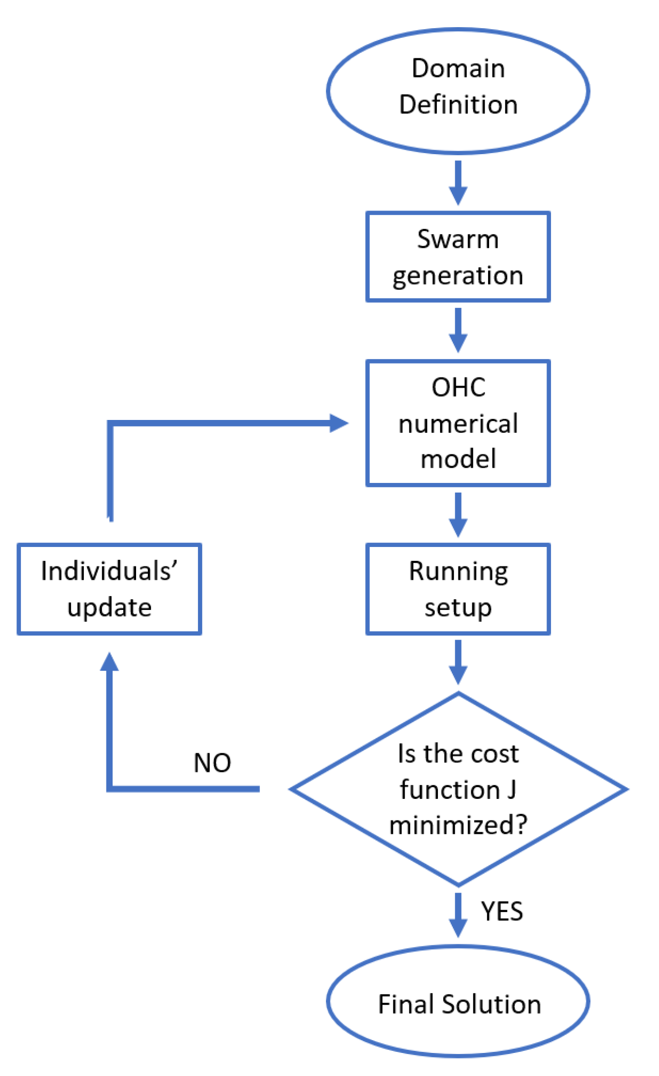
Figure 9.
PSO targeting the experimental measurements [27] of the discharge voltage as function of mass flow rate at 2A.
Figure 9.
PSO targeting the experimental measurements [27] of the discharge voltage as function of mass flow rate at 2A.
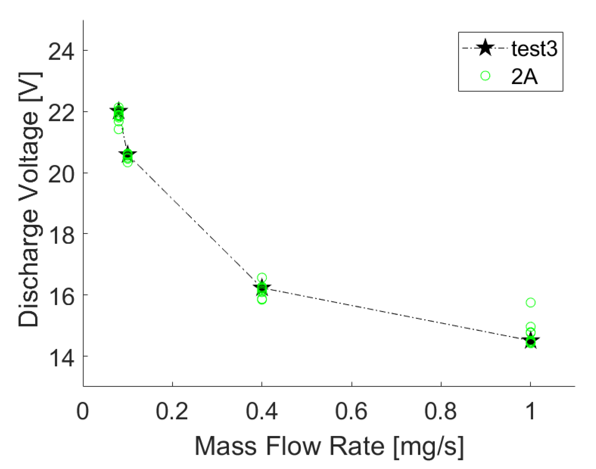
Figure 10.
Emitter Temperature when PSO is targeting the experimental measurements [27] of the discharge voltage as function of mass flow rate at 2A.
Figure 10.
Emitter Temperature when PSO is targeting the experimental measurements [27] of the discharge voltage as function of mass flow rate at 2A.
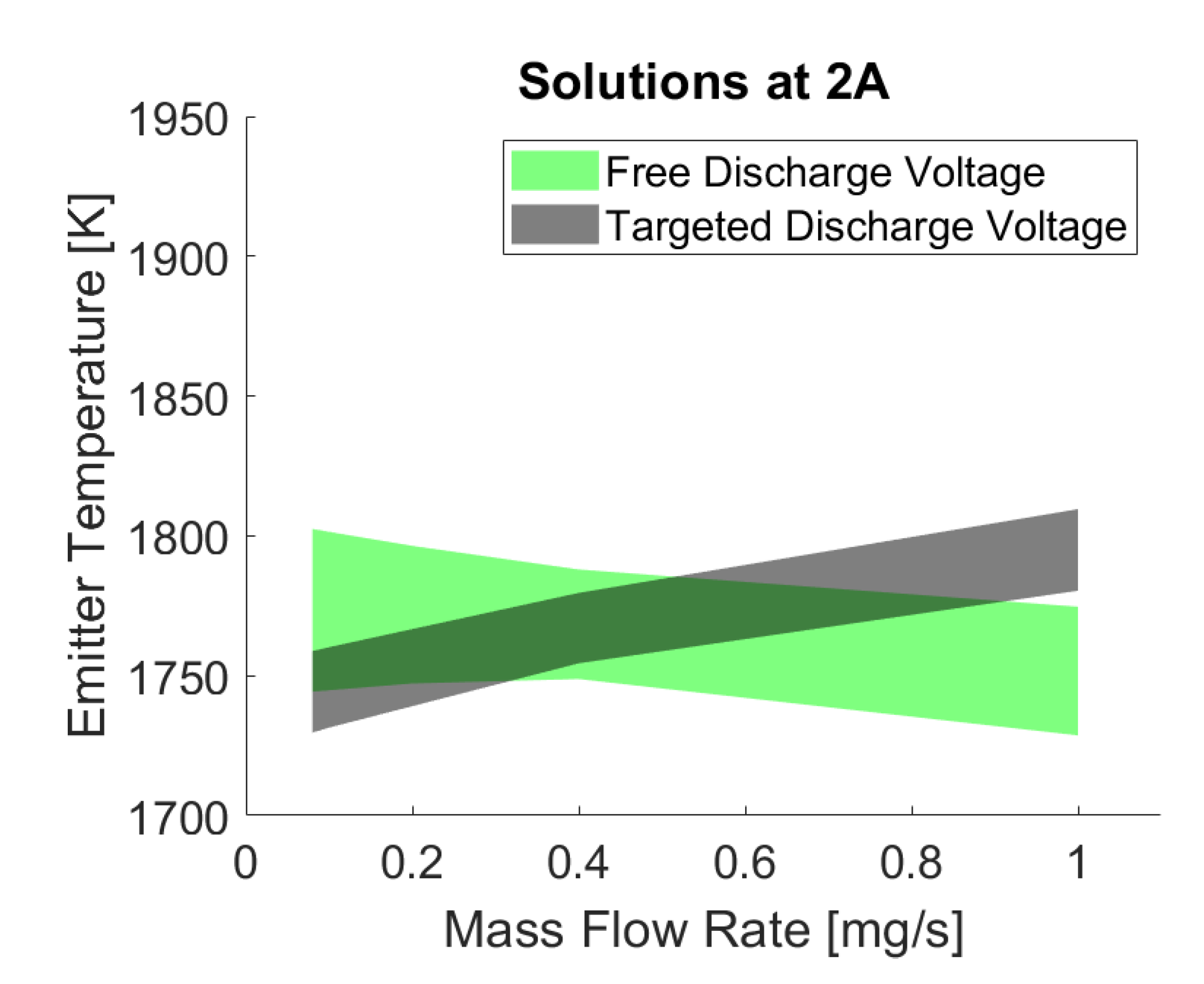

Table 1.
Boundaries of the PSO exploration domain.
| Variable | min | MAX | Unit |
|---|---|---|---|
| 1e21 | 1e24 | ||
| 1e18 | 1e21 | ||
| 5 | 50 | V | |
| 1 | 4 | ||
| 1e21 | 1e23 | ||
| 1e18 | 1e22 | ||
| 1 | 4 | ||
| 1700 | 1950 | K | |
| 1e-3 | 6e-3 | m | |
| 1700 | 1950 | K |
Disclaimer/Publisher’s Note: The statements, opinions and data contained in all publications are solely those of the individual author(s) and contributor(s) and not of MDPI and/or the editor(s). MDPI and/or the editor(s) disclaim responsibility for any injury to people or property resulting from any ideas, methods, instructions or products referred to in the content. |
© 2024 by the authors. Licensee MDPI, Basel, Switzerland. This article is an open access article distributed under the terms and conditions of the Creative Commons Attribution (CC BY) license (http://creativecommons.org/licenses/by/4.0/).
Copyright: This open access article is published under a Creative Commons CC BY 4.0 license, which permit the free download, distribution, and reuse, provided that the author and preprint are cited in any reuse.


