
Submitted:
16 September 2025
Posted:
17 September 2025
You are already at the latest version
Abstract
CREATE-FXB is a Finite Element Method solver specifically developed to address the fixed-boundary problem, namely the determination of the Magnetohydrodynamic equilibrium of an axisymmetric plasma confined within a toroidal nuclear fusion device. Although several solvers are already available and widely used, CREATE-FXB repre-sents a valuable alternative with further improvements, as it introduces a set of dis-tinctive capabilities that extend its applicability and accuracy in modelling this class of problems. Its key features include the design of plasma scenarios in tokamaks, the derivation of linearized plasma response with high accuracy, the treatment of a wide class of current density profiles including non-smooth distributions, and an improved capability of interfacing with other existing codes.
Keywords:
nuclear fusion
; tokamaks
; magnetohydrodynamics
; fixed boundary problems
; finite element methods
; optimization problems
1. Introduction
Numerical models solving the Grad-Shafranov equation in magnetically confined toroidal plasmas are crucial both for the design phase of plasma scenarios [1] and for the development of active magnetic control systems [2]. For these applications, a variety of procedures and associated codes for the calculation of Magnetohydrodynamic (MHD) equilibria are widely used [3,4,5,6,7,8], offering an adequate trade-off between computational efficiency and precision.
In tokamaks, a fixed-boundary equilibrium problem assumes a known plasma shape as input, whereas a free-boundary equilibrium problem simultaneously provides both the plasma shape and internal equilibrium conditions as results. Fixed-boundary problems are computationally simpler and faster, while free-boundary problems are typically employed to test plasma control system performance and analyse experimental data.
The present work focuses on fixed-boundary problems. This approach reduces computational effort, as only the plasma region is meshed, i.e., where the Grad-Shafranov equation needs to be solved. Furthermore, it enables the determination of the plasma response to external poloidal fields without explicitly defining the external coil system. Consequently, it can be used to obtain linearized plasma response to any geometry and number of poloidal field coils, improving flexibility.
This paper presents a new tool called CREATE-FXB, a Finite Element Method (FEM) solver for fixed-boundary problems. The code incorporates several features that make it particularly suited for tokamak applications, including the design of plasma scenarios, high-accuracy derivation of linearized plasma responses, treatment of a wide class of current density profiles (including non-smooth distributions), and improved interoperability with other existing codes. CREATE-FXB employs an innovative nodal numerical formulation, which allows for the treatment of generic current density profiles provided by transport codes [9,10], including profiles with points of non-regularity, in both fixed-boundary problem resolution and subsequent linearization. An optimization tool is also included for estimating the equilibrium currents once the geometry of the magnetic system is fixed.
The paper is organized as follows. Section 2 describes the main assumptions. Section 3 presents the Grad-Shafranov equilibrium equation and its numerical resolution with the formulation used by CREATE-FXB. Section 4 illustrates some applications of the procedure. Finally, Section 5 draws the conclusions and discusses potential future developments compatible with the model.
2. Assumptions
2.1. Basic Equations
At a generic point of the plasma region , static (zero plasma velocity v=0) and stationary (∂/∂t=0) plasma equilibria are well described by the following basic equations below, obtained by means of simplifications of the more complex MHD model [11]:
where is the current density, is the magnetic field, is the vacuum magnetic permeability assumed in the plasma, and p is the kinetic pressure.
Under the 2D axisymmetric assumption in a cylindrical reference coordinate system , using Ampere’s law (1) and the divergence-free condition for the magnetic field (2), both and can be expressed in terms of two scalar functions, the magnetic poloidal flux per radian function and poloidal current function :
where is a 2nd order elliptic operator defined by:
Referring to the plasma region , by substituting (4) and (5) into the (3) and noting that (5) implies:
the Grad-Shafranov (G-S) equation is derived:
The functions and are named free functions.
In the fixed boundary problems, the differential problem is closed by coupling the PDE to some Dirichlet boundary conditions at the plasma boundary :
The problem resolution requires the expression of . Thus, the free functions must be assigned or derived in some way.
2.2. Current Density Modelling
The current density modelling passes through the derivation of the free functions and . Usually, they are given as function of the non-dimensional variable defined as follows:
where and are the values of the flux per radian at the magnetic axis and at the plasma boundary, respectively.
These functions can be obtained by coupling a simplified one-dimensional version of the Grad-Shafranov equilibrium to the transport equations [9,10], adopting iterative schemes to solve the non-linear system and derive the plasma pressure and poloidal current function . Afterwards, these profiles are given to specific 2D axisymmetric codes coupled to circuit equations like CREATE-NL+ [5] to get the time evolution of the poloidal flux map.
An alternative procedure takes and from suitable family of functions . The variable is a set of shape parameters necessary to model the features of the current density profile as shown in [12]. They represent the degrees of freedom of the parameterization , linked to the main plasma quantities, namely plasma current , poloidal beta , and internal inductance , which can be defined as follows:
where is the magnetic field component in the poloidal plane .
However, different definitions of and can also be employed [13]. The choice of this parameterization is motivated by the fact that the flux surfaces outside the plasma boundary are nearly identical for two equilibria with different current density profiles but the same values of , and [14]. Therefore, the magnetic coupling of the plasma with the external conductors can be modelled by means of a suitable choice of the parameters.
These parameters are calculated using iterative methods, i.e., by solving (7)-(9) until the desired values of plasma quantities (11) are obtained. The computational effort depends on the number of degrees of freedom (DoFs). Therefore, the choice of should be made so as to ensure coverage of the widest possible range of plasma quantities with a limited amount of computational effort.
Several methods have been proposed to model the current density profile in terms of . For instance, power functions can be employed for both and , as in the CREATE-L code [5], which usually implements a formulation featuring three DoFs:
which corresponds to bell-shaped current density profiles due to the term This bell-shaped expression is relatively simple, but it cannot be used for plasma equilibria characterized by low values of , where the current density typically exhibits a hollow profile and tends to concentrate near the boundary. A new family of functions must be determined to be non-monotonic with for specific values of α correspondent to a low internal inductance. Moreover, it should be as simple as possible, to guarantee convergence with sufficient rate.
The CREATE-FXB code can also use the following parameterization in terms of the four parameters , derived by modifying the McCarthy class of profiles [15]:
which enables the treatment of a wide class of plasmas, as shown in Section 4. It is worth noticing that the filter function plays a key role in shaping the plasma current density.
In some cases, the profiles both and provided by transport codes may be highly rough and irregular. Examples of treatment of this kind of profiles are also shown in Section 4, where an innovative technique based on information from the mesh nodes has been adopted.
All these features represent a challenge more for the linearization procedure than for the numerical resolution of the fixed boundary problem: indeed, the coupling between standard FEM with linear triangular elements with iterative fixed-point scheme (Picard iterations) is quite robust to face the non-linearity in the computation of the plasma equilibrium quantities. On the other hand, the derivation of the linearised model becomes challenging, because the linearization involves the numerical calculation of profiles derivatives, which cannot be rigorously evaluated in the non-regularity points. For these reasons, adequate meshing processes and suitable numerical techniques to treat the irregularities of the profile are crucial for derivation of the linear model. In this context, the so-called nodal formulation, a numerical technique formalized in the subsequent paragraphs, which represents a suitable way to overcome the limitations of conventional methods. Additionally, a procedure of adaptive refinement of mesh can also be used.
3. Finite Element Method Formulation in CREATE-FXB
3.1. Picard Iterations
Equation (8) is a non-linear elliptical partial differential equation, perfectly suited for the resolution using the standard FEM. The first step is to convert it into the weak formulation, by multiplying all the members by a weight function and applying integration by parts:
The non-linearity appears in the right-hand side, since the toroidal current density depends on the unknown .
The plasma domain is discretized into a set of triangular elements with N nodes, corresponding to the vertices of the triangles. The unknown solution is approximated via a linear combination of shape functions :
where at the -th node, is zero at the other nodes, and is piecewise linear within the elements containing the l-th node.
The unknown variable can thus be represented as a numerical vector of length N rather than as a function, so that independent equations are required to find the solution. These are obtained from weak formulation (14) by applying Galerkin’s approach, which selects :
which, in a compact form, become the matrix relation:
where:
At this point, Dirichlet’s boundary conditions must be imposed on (17), according to (9). In this case the last term , which would be needed in case of Neumann boundary conditions, becomes redundant. To this end, the set of nodes is partitioned into two subsets: corresponding to internal nodes, and of internal and boundary nodes, marked by indices ii and ib, respectively. The same operation is done for the nodal values of . In system (17) K is then rewritten in block format:
where clearly due to properties of functions, can be ignored since only the first subset of equations is required for the next step, is known (Dirichlet’s boundary condition) and depends on .
Therefore, a Picard scheme is adopted to solve the non-linearity, with the unknown vector uniquely determined by solving, at each step :
until a convergence criterion is satisfied.
Additional information on the well-posedness of system (17) can be found in [16].
3.2. Nodal Formulation for
A critical aspect in solving the Grad–Shafranov equation is the accurate evaluation of the current density , especially in the presence of steep gradients or discontinuities in the equilibrium profiles. Standard approaches use linear triangular elements and Gauss integration, e.g., in the CREATE-NL+ code [5], where the term in (18) is computed iteratively from the values of and the shape functions in each triangle barycentre as well as the map is determined in these points, while the free function values are read from the diagrams and . However, the main issue arises when the profiles present discontinuities. In such cases, if the level at which is discontinuous falls into a bend of elements, the integrals are done with a wrong value of . To address this limitation, a nodal formulation is introduced, in which the current density is reformulated in terms of nodal quantities, ensuring a smoother and more robust treatment of discontinuities.
The main issue arises when the profiles present discontinuities. In such cases, if the level at which is discontinuous falls into a bend of elements, the integrals are calculated with a wrong value of .
In order to properly handle the high steep current density regions within the plasma domain, as well as the possible discontinuities of respect to , the current density is reformulated as follows:
where and , are computed from and defined at the mesh nodes according to their respective profile functions. In this way, spatial discontinuities resulting from discontinuities in and are smoothed out. As a result, the computation of (the flux source) becomes more accurate, and consequently, so does the evaluation of the flux itself. The singularity in the right-hand side of (21) wherever can easily be handled. Indeed, the flux gradient is typically zero for well defined values of , namely at the magnetic axis () and at the null points at the plasma boundary ().
The nodal formulation is particularly suited in two cases that are beyond the scope of this paper, namely:
- the free boundary problem in cases where the current density is non-zero at the plasma edge;
- the derivation of the linearized plasma response to external currents and profile variations.
3.3. Accurate Calculation of the Magnetic Flux and Field
The above MHD equilibrium calculation with linear triangles provides a piecewise constant value of the flux gradient and yield magnetic field discontinuities across elements.
To tackle these issues, especially when the derivative of the magnetic field is needed, two different actions are undertaken. The first action is a mesh refinement wherever the discontinuities in the flux gradient and/or the gradients of the current density exceed prescribed thresholds.
The other method is a post-processing algorithm that requires very limited computational effort while ensuring the regularity of field derivatives, which is crucial for certain applications. This method is based on Helmholtz’s theorem [17] and employs the finite element method (FEM) with linear shape functions to calculate and in the second order calculation. With the technique proposed in [18], the poloidal magnetic field can be determined by post-processing the standard FEM flux map as the solution to the minimization problem:
where, from (4), , while are suitable non-dimensional constants.
The quantities , and , which is the tangential component of , are obtained from the first order FEM solution of the G-S equation. This formulation ensures continuity and achieves a convergence rate of order O(h2) also for , where h is the mesh size. These properties are highly useful, offering a high level of accuracy and enabling the derivation of reliable linearized models with limited computational effort, especially when compared to other methods, such as [19].
3.4. Optimization of Poloidal Field Coil Currents
The optimization of the number, position and dimension of the Poloidal Field (PF) coils in a tokamak is a challenging task, due to linear and nonlinear constraints related to maintenance requirements, and technological limits on electric power, current density, magnetic fields, and vertical forces [8,9,10,11,20]. Here, the problem of the optimization of the currents of the PF coils in air core tokamaks while keeping their positions fixed has been addressed [4,5,6,7]. It is based on the linearization of the GS equation around the desired plasma equilibrium. An iterative optimization problem, subject to both linear and quadratic constraints, is then solved.
The total flux per radian at the plasma boundary is the sum of two terms:
Here , the flux pre radian due to the PF coils, can readily be computed using Green functions based on elliptic integrals [21]. The calculation of the plasma contribution using elliptic integrals may be cumbersome, since the boundary is in contact with the source currents. A solution, having the same degree of accuracy as FEM can be obtained by surrounding the fixed mesh boundary (i.e., the plasma contour) with a halo region made of a few layers of elements, and solving:
where is given by the solution of Section 2.1 in , and vanishes in .
The boundary condition on is computed using Green functions from . This method gets rid of the singularities, since the minimum distance between the points of the boundary and the sources is the thickness of the layer.
The PF coil currents are then optimized using one of the methods described in [8,9,10,11,20]. Since the optimized flux per radian is hardly equal to the difference between and , it is necessary to check whether the free boundary equilibrium is sufficiently close to the desired fixed boundary configuration. This task is fulfilled by a specific version of the CREATE-NL+ code, solving the free boundary equilibrium code in a semicircle of the rz plane in the first and fourth quadrants, adding further elements to the mesh used for solving the fixed boundary problem. In this version of the free boundary code, the PF equilibrium currents are treated as a set of filaments at the same locations used for Gauss integration of elliptic integrals.
3.5. Linearization
The formulation described in this paper can effectively be used to derive a linearized plasma response model. The description of the details of the linearization procedure is outside the scope of the present paper. However, it is worth noticing that linearized models obtained with this procedure are extremely accurate and can efficiently be employed for plasma identification, magnetic control, and optimization of PF coil current waveforms.
4. Results and Discussion
This section shows the flexibility of parameterization (13) and demonstrates the reliability of the CREATE-FXB code with a number of benchmark cases, obtaining a very good agreement with available analytical solutions and other numerical results in the literature.
4.1. Envelopes for Current Density Parameterization
This section compares the limits of validity of three parameterization choices for the current density in the - plane for an elliptic plasma (Figure 1a).
The CREATE-FXB parameterization proposed here in (13) is able to obtain plasmas with a wide range of and values. Figure 1 shows that the upper bounds (more than 20 for and more than 4 for ) are clearly larger than those obtained with the other parameterizations. As stated in Section 2, the CREATE-FXB parameterization (13) is also able to obtain low values of , i.e., down to about 0.2 like McCarthy’s family, whereas the corresponding lowest value for CREATE-L is about 0.5.
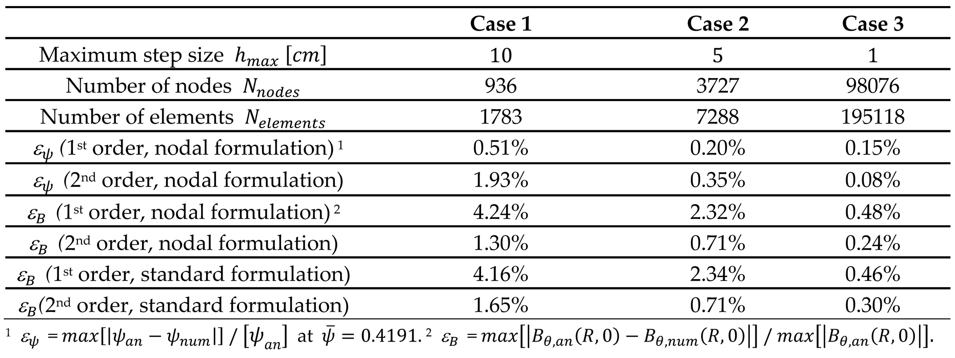
4.2. Circular Plasma with a Large Aspect Ratio and Discontinuous Current Density Profile
The robustness of the nodal formulation is shown by comparing the standard and new numerical solutions with the analytical one, in a case with a very large aspect ratio and a discontinuous current density profile. The test case is hence a circular plasma with a minor radius , a major radius , and current density profile defined by:
This 1D problem, which has a straightforward analytical solution, is solved as a 2D problem using FEM. Figure 2 shows the azimuthal field in the plasma region evaluated both using the standard and the nodal formulation of the current density in the numerical solver. Moreover, for each formulation, the 2nd order procedure has been applied.
Two aspects are highlighted in Table 1, which reports the values of the numerical error. Firstly, the nodal formulation provides better results when the discretization is coarse. Secondly, higher accuracy and smoothness of the magnetic field is obtained by post-processing the FEM solution with the method introduced in [18] and summarized in Section 3.3, no matter about the involved formulation.
4.3. Non-Circular Low Aspect Ratio Plasma Equilibrium
The procedure has been applied also to a low-aspect ratio plasma equilibrium with an available analytical solution. The reference case is described in [22], with
where is the poloidal flux per radian at the magnetic axis, is the radial coordinate of the magnetic axis, and is a non-dimensional constant (there is a typo in [22] in the exponent of .
The analytic solution of the Grad-Shafranov equation is given by:
By fixing the previous parameters as follows:
and choosing as boundary flux per radian:
the coordinates of the separatrix are shown in Figure 3a.
In this case the nodal and the standard formulations yield exactly the same results, since the current density is linear in each triangular element. Figure 3b shows the trend of the numerical error on the flux with the infinity norm as a function of the maximum element size , which scales with , as shown in [16].
4.4. Optimization of PF Equilibrium Currents in DTT
The fixed boundary solver has been used to determine the set of PF current needed to keep in equilibrium a single plasma in DTT.
Figure 4 shows the target plasma boundary at 27 s in the DTT plasma scenario with =5.5 MA, , , and [23]. The CREATE-FXB code has firstly calculated the fixed boundary equilibrium in , and then the flux per radian due to the plasma , obtained in the region , using the procedure described in Section 3.4.
Afterwards, the CREATE-FXB code minimizes , which is the difference between (flux per radian due to the PF system at the plasma boundary) and the desired equilibrium value, namely - . The PF system includes 12 circuits and 24 coils. The details are given in [23]. Figure 5a shows the as a function of the maximum current in the circuits . Figure 5b shows the optimal currents in comparison with those reported in [23]. The slight improvement of CREATE-FXB is due to a different choice of the figure of merit, since the procedure used in [23] optimizes the entire scenario adding further constrains.
The validity and the effectiveness of the CREATE-FXB procedure is in any case demonstrated in Figure 5c, where the free boundary equilibrium obtained by the CREATE-NL+ code using the PF circuit currents obtained by CREATE-FXB provides a plasma boundary almost coincident with the desired shape, since the maximum distance is less than 9 mm.
5. Conclusions
In this work, CREATE-FXB is presented as a new fixed-boundary solver for the Grad–Shafranov equation, based on the Finite Element Method with an innovative technique. The code provides an efficient and accurate tool for plasma equilibrium analysis in tokamaks, offering robust handling of non-smooth current density profiles, second-order accuracy in the evaluation of magnetic flux and field, and an integrated framework for PF coil current optimization.
Validation against the free-boundary code CREATE-NL+ has confirmed the reliability of the approach for scenario design and equilibrium current estimation. Future extensions will focus on the systematic use of the derived linearized models for plasma identification and control, on the integration of plasma response-based scenario optimization strategies.
Overall, CREATE-FXB constitutes a flexible and accurate complement to the CREATE code family, enhancing its capability to address fixed-boundary problems in tokamak applications.
Author Contributions
Conceptualization, Raffaele Albanese (R.A.), Marco Neri (M.N.) and Pasquale Zumbolo (P.Z.); methodology, R.A., M.N. and P.Z.; software, R.A., M.N. and P.Z ; formal analysis, R.A., M.N. and P.Z ; investigation, R.A., M.N. and P.Z ; resources, R.A., M.N. and P.Z ; data curation, R.A., M.N. and P.Z ; writing—original draft preparation R.A., M.N. and P.Z ; writing—review and editing, R.A., M.N. and P.Z ; supervision, R.A.; project administration, R.A.; funding acquisition, R.A.. All authors have read and agreed to the published version of the manuscript.
Funding
This work was supported in part by the PRIN Project P2022KNM7B “TRAINER - Tokamak plasmas daTa-dRiven identificAtIon and magNEtic contRol”, CUP E53D23014670001 funded by EU in NextGenerationEU plan through the Italian “Bando Prin 2022 - D.D. 1409 del 14-09-2022” by MUR. This work was also partially supported by the Italian Research Ministry under the PRIN Project 2022JCZJ33”. Advanced control techniques for the alternative divertor plasma configurations in nuclear fusion tokamaks”, CUP: E53D23000670006.
Conflicts of Interest
The authors declare no conflicts of interest.
References
- Mattei, M., Albanese, R., Ambrosino, G., & Portone, A. (2006, December). Open loop control strategies for plasma scenarios: linear and nonlinear techniques for configuration transitions. In Proceedings of the 45th IEEE Conference on Decision and Control (pp. 2220-2225). IEEE.
- Mele, A., Albanese, R., Ambrosino, R., Castaldo, A., De Tommasi, G., Luo, Z. P., ... & Xiao, B. J. (2019). MIMO shape control at the EAST tokamak: simulations and experiments. Fusion Engineering and Design, 146, 1282-1285.
- Albanese, R., Blum, J., & De Barbieri, O. (1987, September). Numerical studies of the Next European Torus via the PROTEUS code. In 12th Conf. on Numerical Simulation of Plasmas, San Francisco.
- Albanese, R., & Villone, F. (1998). The linearized CREATE-L plasma response model for the control of current, position and shape in tokamaks. Nuclear Fusion, 38(5), 723.
- Albanese, R., Ambrosino, R., & Mattei, M. (2015). CREATE-NL+: A robust control-oriented free boundary dynamic plasma equilibrium solver. Fusion Engineering and Design, 96, 664-667.
- Miki, N., Verrecchia, M., Barabaschi, P., Belov, A., Chiocchio, S., Elio, F., ... & Utin, Y. (2001). Vertical displacement event/disruption electromagnetic analysis for the ITER-FEAT vacuum vessel and in-vessel components. Fusion engineering and design, 58, 555-559.
- Portone, A. (2004). Perturbed solutions of fixed boundary MHD equilibria. Nuclear fusion, 44(2), 265.
- Lazarus, E. A., Lister, J. B., & Neilson, G. H. (1990). Control of the vertical instability in tokamaks. Nuclear Fusion, 30(1), 111.
- Pereverzev, G. V., & Yushmanov, E. P. (2002). ASTRA. Automated System for TRansport Analysis in a tokamak.
- Khayrutdinov, R. R., & Lukash, V. E. (1993). Studies of plasma equilibrium and transport in a tokamak fusion device with the inverse-variable technique. Journal of Computational Physics, 109(2), 193-201.
- J.P. Freidberg, Ideal magnetohydrodynamic theory of magnetic fusion systems, (1982) Reviews of Modern Physics, 54 (3), pp. 801 - 902, DOI: 10.1103/RevModPhys.54.801. [CrossRef]
- Lao, L. L., John, H. S., Stambaugh, R. D., Kellman, A. G., & Pfeiffer, W. (1985). Reconstruction of current profile parameters and plasma shapes in tokamaks. Nuclear fusion, 25(11), 1611.
- Wesson, J. &Campbell, D.J. (2004). Tokamaks. ISBN 9780198509226, Clarendon Press.
- Luxon, J. L., & Brown, B. B. (1982). Magnetic analysis of non-circular cross-section tokamaks. Nuclear Fusion, 22(6), 813.
- Mc Carthy, P. J. (1999). Analytical solutions to the Grad–Shafranov equation for tokamak equilibrium with dissimilar source functions. Physics of Plasmas, 6(9), 3554-3560.
- Quarteroni, A. (2006). Il metodo di Galerkin-elementi finiti per problemi ellittici. Modellistica numerica per problemi differenziali, 37-96.
- Neittaanmäki, P., & Saranen, J. (1981). On finite element approximation of the gradient for solution of Poisson equation. Numerische Mathematik, 37(3), 333-337.
- Albanese, R., Iaiunese, A., & Zumbolo, P. (2023). Solution of Grad-Shafranov equation with linear triangular finite elements providing magnetic field continuity with a second order accuracy. Computer Physics Communications, 291, 108804.
- Jardin, S. C. (2004). A triangular finite element with first-derivative continuity applied to fusion MHD applications. Journal of Computational Physics, 200(1), 133-152.
- Albanese, R., Ambrosino, R., Castaldo, A., & Loschiavo, V. P. (2018). Optimization of the PF coil system in axisymmetric fusion devices. Fusion Engineering and Design, 133, 163-172.
- Byrd, P. F., & Friedman, M. D. (2013). Handbook of elliptic integrals for engineers and physicists (Vol. 67). Springer.
- Schnack, D.D.: Toroidal Equilibrium; The Grad–Shafranov Equation. Lect. Notes Phys. 780, 107–120 (2009) c Springer-Verlag Berlin Heidelberg 2009. doi:10.1007/978-3-642-00688-3 18.
- Castaldo, A.; Albanese, R.; Ambrosino, R.; Crisanti, F. Plasma Scenarios for the DTT Tokamak with Optimized Poloidal Field Coil Current Waveforms. Energies 2022, 15, 1702. [Google Scholar] [CrossRef]
Figure 1.
Limits of validity of three parameterization choices and envelopes in βpol-li plane: a) plasma shape and FEM mesh; b) McCarthy parameterization [15]; c) CREATE-L parameterization [5]; d) CREATE-FXB parameterization proposed here in (13).
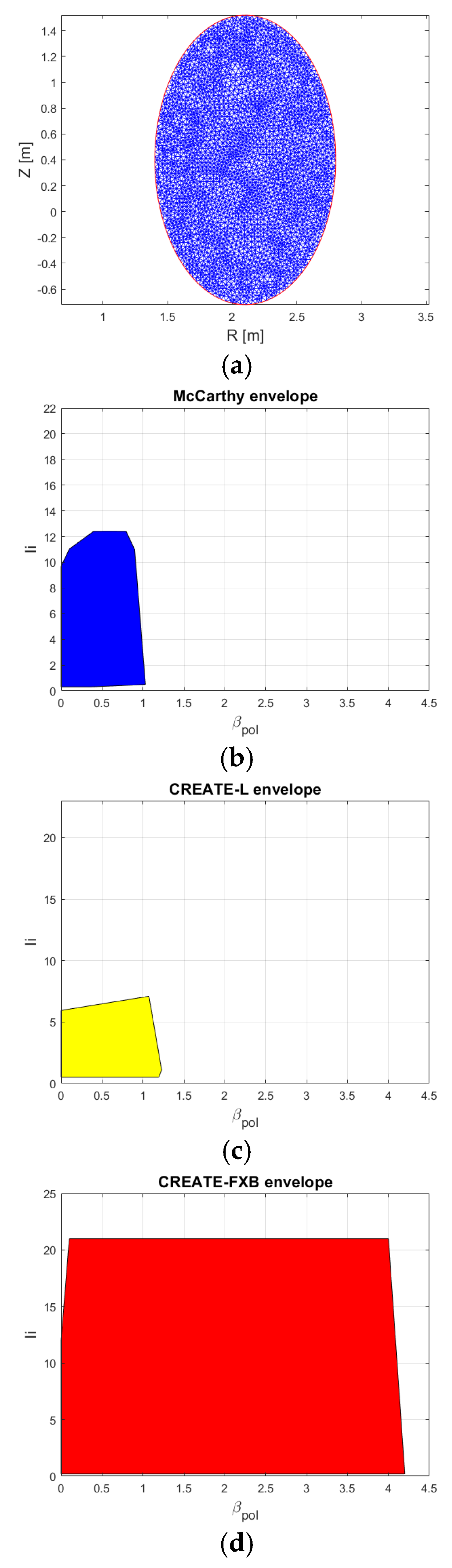
Figure 2.
Analytical and numerical evaluation of the azimuthal magnetic field Bθ along the pinch radius R∈[0,1 m] at Z = 0: a) FEM mesh, with 936 nodes and 1783 elements; b) profile; c) comparison between the classic 1st and 2nd order magnetic field solutions, using the nodal and the standard formulation of Jϕ; (c) zoom at R∈[0.4,1] m,Bθ∈[0.15,0.32] T.
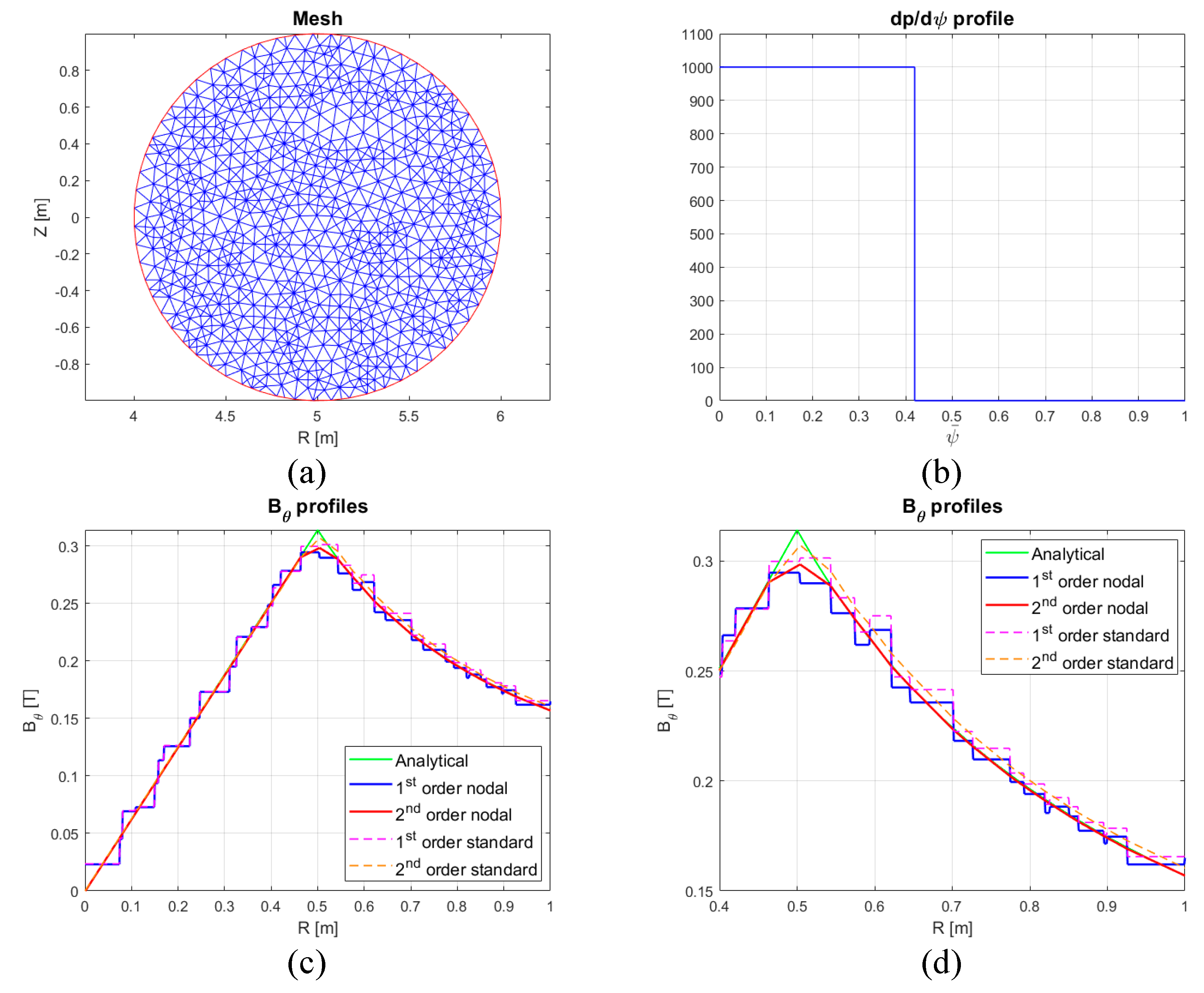
Figure 3.
Non-circular low aspect ratio plasma equilibrium. Comparison between numerical and analytic solution: a) analytical flux levels inside the plasma region; b) trend of the relative error on the poloidal flux per radian 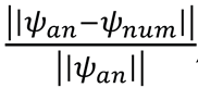 , with ψ at the mesh nodes; c) Bθ profile along the line at Z = 0; d) numerical error on the magnetic field
 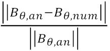 at Z = 0.
, with ψ at the mesh nodes; c) Bθ profile along the line at Z = 0; d) numerical error on the magnetic field at Z = 0.
Figure 3.
Non-circular low aspect ratio plasma equilibrium. Comparison between numerical and analytic solution: a) analytical flux levels inside the plasma region; b) trend of the relative error on the poloidal flux per radian , with ψ at the mesh nodes; c) Bθ profile along the line at Z = 0; d) numerical error on the magnetic field at Z = 0.
, with ψ at the mesh nodes; c) Bθ profile along the line at Z = 0; d) numerical error on the magnetic field at Z = 0.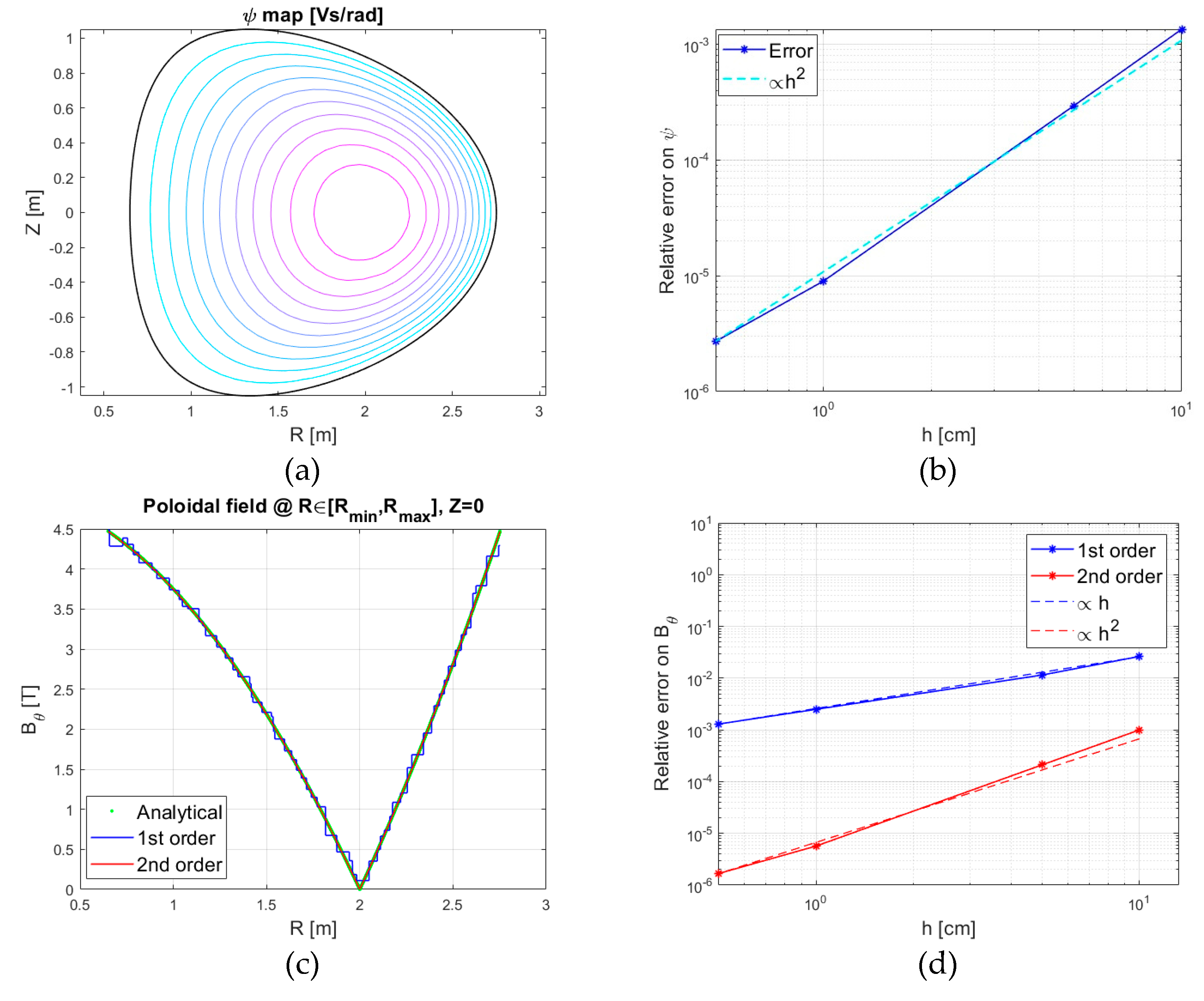
Figure 4.
Target plasma boundary at 27 s in the DTT plasma scenario with Ipl=5.5 MA, ψ=0.70 Vs/rad, βpol=0.10, and li=0.80 [23]: a) fixed boundary solution obtained by CREATE-FXB in Ωpl, ; b) ψpl (flux per radian due to the plasma) in Ωpl ∪ Ωh.
Figure 4.
Target plasma boundary at 27 s in the DTT plasma scenario with Ipl=5.5 MA, ψ=0.70 Vs/rad, βpol=0.10, and li=0.80 [23]: a) fixed boundary solution obtained by CREATE-FXB in Ωpl, ; b) ψpl (flux per radian due to the plasma) in Ωpl ∪ Ωh.

Figure 5.
PF circuit current optimization in DTT plasma scenario at 27 s: a) minimum value of the discrepancy between PF flux per radian and its desired value as a function of the maximum circuit current; b) optimal currents in comparison with those reported in [23]; c) desired shape and plasma edge provided by the free boundary CREATE-NL+ code using the circuit currents provided by CREATE-FXB (the maximum distance is less than 9 mm).
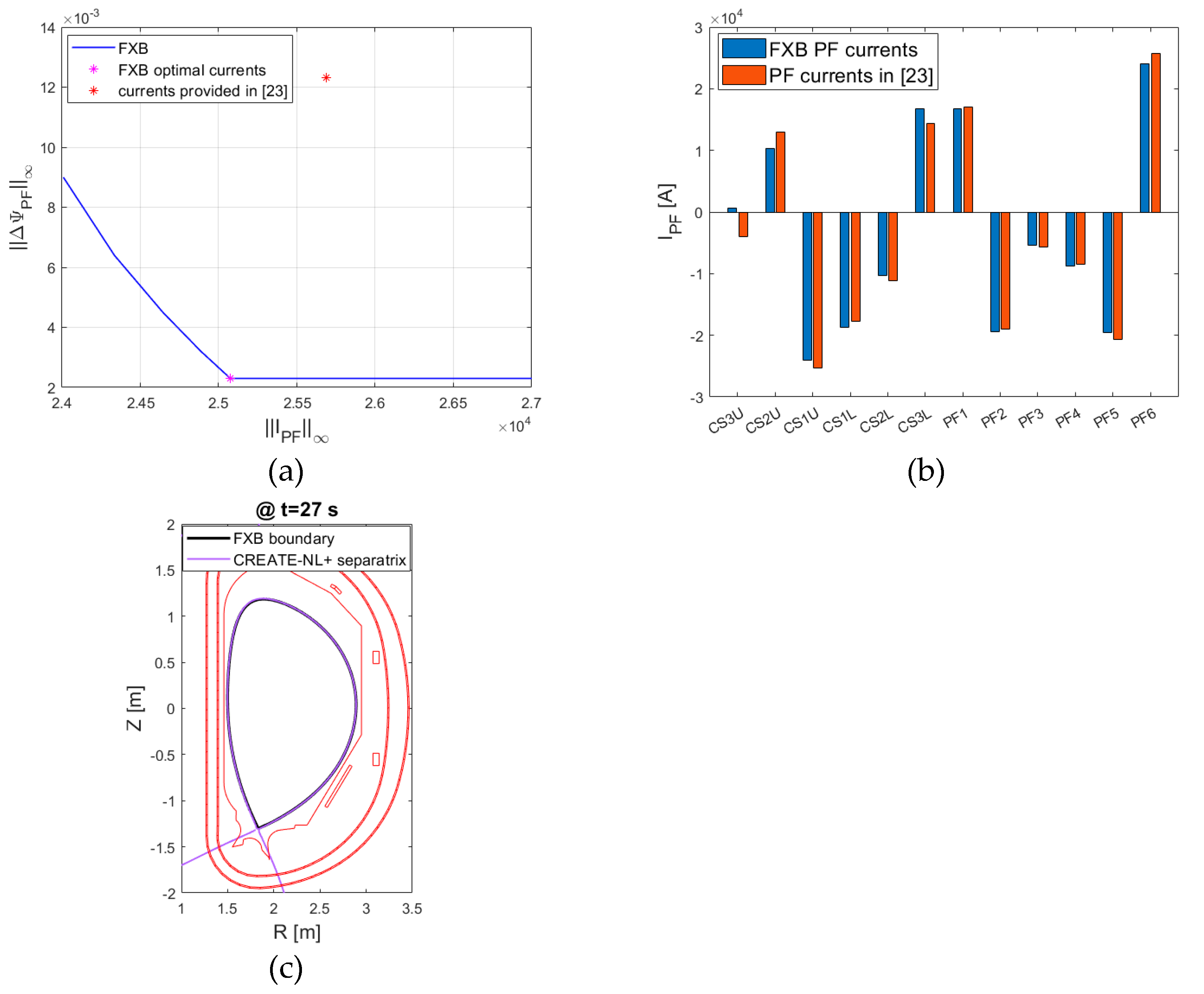

Table 1.
Circular plasma with a large aspect ratio and discontinuous current density profile: numerical errors.
Table 1.
Circular plasma with a large aspect ratio and discontinuous current density profile: numerical errors.
 |
Disclaimer/Publisher’s Note: The statements, opinions and data contained in all publications are solely those of the individual author(s) and contributor(s) and not of MDPI and/or the editor(s). MDPI and/or the editor(s) disclaim responsibility for any injury to people or property resulting from any ideas, methods, instructions or products referred to in the content. |
© 2025 by the authors. Licensee MDPI, Basel, Switzerland. This article is an open access article distributed under the terms and conditions of the Creative Commons Attribution (CC BY) license (http://creativecommons.org/licenses/by/4.0/).
Copyright: This open access article is published under a Creative Commons CC BY 4.0 license, which permit the free download, distribution, and reuse, provided that the author and preprint are cited in any reuse.


