

Submitted:
19 June 2024
Posted:
20 June 2024
You are already at the latest version
Abstract
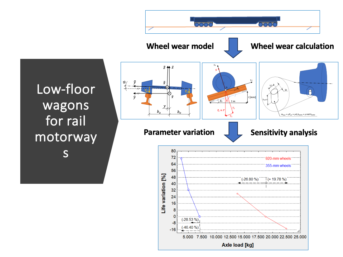
This paper shows the usage of a numerical analysis model which enables the calculation of the life of a railway wheels used for low-floor freight wagons as a function of its primary operating factors, which allows carrying out sensitivity analyses. Low-floor wagons are being increasingly used for combined transport applications and many types of bogies have been proposed in order to constitute the wagons. Due to the uniqueness of this type of wagons, the bogie configurations in terms of wheelbase and axle load have hardly been analyzed so far. The numerical analysis model used addresses the primary challenges that arise in the vehicle – track interaction and establish the relations among them. The main aspects of this model have been described in the paper, which has been later used to calculate the life of an ordinary-diameter wheel for several wheelbase and axle load values. This study has been replicated with reduced-diameter wheels, which are commonly used for low-floor wagons. In this way, it is possible to know the evolution of the life depending on the wheelbase and the axle load. The root causes underlying the observed behaviors can be explained by the entire understanding of the rolling phenomenon provided by the full analytical work.
Keywords:
sensitivity analysis
; vehicle-track interaction
; freight transport
; sustainable transport
; rail motorway.
1. Introduction
The objective of this work is to determine the sensitivity of the wheelbase and axle load in wheel wear, which allows finding out convenient configurations for the bogies with which low-floor wagons are equipped. For that, a calculation model able to determine the life of a wheel as a function of its primary operating factors is used. The model allows varying the wheel diameter as well, which makes it possible to compare different types of wheels commonly found on these wagons.
Nowadays, the needs in the field of logistics are changing and new transportation models are arising. One of the models that is becoming more popular in the last years is the rail motorway model, which consists in transporting whole freight articulated vehicles on railway wagons. This model cuts down CO2 emissions, saves fuel, reduces road congestion and may be more profitable than road transportation for some routes. It can also be used to skip certain obstacles, harsh routes or remote-access zones (Fomento, 2018). The concept of loading the whole heavy-duty vehicle avoids breakbulk shipping whereas it brings the loading and unloading time down to 1 minute, since the vehicles can run on / off board the wagons quickly and then their wheels are secured quickly as well (Jaro & Folgueira, 2012). Figure 1 shows a schematic diagram of this concept:
Notwithstanding, the adoption of this model often encounters the problem of loading gauge. Due to the height of the articulated vehicles used for road transportation, around 4 m (European Council, 1996), placing them on wagons leads to a further height increase over the rails that may conflict with the height limitations found in some tunnels or under some overpasses. Figure 2 illustrates this conflict:
In order to avoid interferences between the load (the heavy-duty vehicles) and the civil structures (tunnels and overpasses found in the railway route) and keep transporting those road vehicles, there is one economically-feasible alternative, as it does not require any civil works on the route: lowering the loading plane height. As it can be seen in Figure 2, this height depends on the wheel diameter among other factors, so it can be lowered by using reduced-diameter wheels (Jaro & Folgueira, 2012).
An ordinary wheel has about 920-mm diameter, while a reduced-diameter wheel has a diameter value between half and third of the ordinary one. From this variety of wheels, another variety of bogie originates: the wheels can be arranged on the bogies with different wheelbases, and they can be loaded more or less intensely, which along with the number of axles determines the axle load.
For that, the calculation model sought must take into account many railway factors involved in vehicle – track interaction. These parameters can be grouped so: wheel, wagon, railway superstructure and external factors. The process consists in defining a mathematical model under the behavioral equations extracted from the models explaining wheel degradation, each of which includes a set of hypotheses. Additional hypotheses will be formulated so as to take out the least influential factors on degradation. These hypotheses regard significant degradation phenomena as rolling contact fatigue (RCF).
Regarding the vehicle, the infrastructure and their interaction, the work aims to focus on the Spanish conventional railway network. This is because rail motorways are currently being fostered in Spain and this country presents some obstacles to their implementation: the conventional railway network presents an unfavorable loading gauge (Fomento, 2018), which prompts the adoption of low-floor wagons, and, additionally, the tight curves and the steep gradients inflict severe damage to wheels, being possible to mitigate it with smoother operating factors. These wheels are arranged in wheelsets, with a wheelset being the rigid union of an axle with a pair of wheels. Wheelsets are usually arranged in two-axle (two-wheelset) bogies and, according to the same reference, two bogies are enough for a flat-bed (and low-floor) wagon used on a rail motorway, so this is the type of railway vehicle that is to be considered for wheel degradation.
With that being said, the analysis will be limited to freight transport and to the Spanish national railway network, whose track gauge is specific: 1,668 mm. The analysis will exclude external factors just as the weather or the presence of pollutants, as these are fairly volatile and difficult to forecast.
This research paper can be compared to other cutting-edge work on wheel wear calculation, but differs in some significant respects. These differences are commented upon next: To start with, reference (Cui et al, 2016) performs a sensitivity analysis with the key bogie parameters (suspension stiffness and wheel rolling radii difference, mainly) and uses the wear as an indicator, with the goal of reducing wheel flange wear and rail gauge corner wear and, thus, addressing the importance of wheel wear, although the rail vehicle modeled is an electric multiple unit (EMU) and axle load and wheelbase are not tackled. Reference (Corrêa et al., 2023) carries out a sensitivity analysis of the primary suspension longitudinal clearance and stiffness and shows how significantly they can affect wear and increase maintenance costs, yet it does not deal with axle load and wheelbase. Reference (Zhai et al, 2020) shows the importance of addressing uneven wear and its impact on the railway system and the fact that reducing wheel diameter can impact wear patterns and dynamics, which is part of the theoretical foundation of the work hereby presented, which has also performed the variation of axle load and wheelbase, differently to the former work. Reference (Wang et al. 2021) emphasizes the relevance of considering the interaction between wheel and rail materials and their hardness in understanding wear behavior, which has been regarded in the current work, besides performing a sensitivity analysis. Reference (Seo, Hur & Known, 2022) found that the wear rate of materials with large total hardness used for the rail and wheel decreased, indicating a potential correlation between wheel diameter and wear rate, which has been also tackled in the current article, besides undertaking a sensitivity analysis. References (Sang. et al., 2023) and (Soleimani & Moavenian, 2017) stated that controlling and reducing friction and wear rate can be achieved through methods such as lubrication and load regulation, highlighting the effects of acceleration because of the impact of traction torque and creepages (load transfer phenomenon in suspension can make the wheel-rail interaction more intense than at a constant speed), albeit the current work focuses on a sensitivity analysis with real axle load and also wheelbase values. To end with, reference (Yenealem, 2023) simulates wear performance analysis using multibody simulation software and MATLAB and the results indicate that the wheel wear rate increases proportionally with load, however, the work focuses on ordinary-diameter wheels and does not vary the wheelbase values.
The main contribution of this work consists in finding the evolution of wheel wear as a function of its operating factors for low-floor wagons, which has been hardly treated due to their uniqueness. The work is insightful, given that wheel, wheelset and bogie kinematics and dynamics have been analyzed, so it provides comprehension as to why wheel life is not the same regardless of the parameters of interest and why dependencies exist.
Differently to the previous research, several realistic scenarios basing on rail motorways have been proposed and only those parameters of interest have been varied in the procedure of analysis developed, keeping the rest of the procedure the same or with equivalent parameters, which makes comparisons at the same level possible.
Once the analysis procedure has been validated, the methodology is open to changes, so that more factors can be added or some of the behavioral laws can be altered or swapped in future research works in order to improve the accuracy and computational effort of the sensitivity analyses.
To conclude with the introduction, it is worth remarking that in order to carry out this research work it has been necessary to review many analytical models which enable the calculation of wheel wear. Some of these models are based on rolling kinematics, while others are on dynamics. The most recurring references are (Fissette, 2016), (Larrodé, 2007), (Moody, 2014), (Pellicer & Larrodé, 2021), (Oldknow, 2015), (Ortega, 2012), (RENFE, 2020), (Rovira, 2012) and (Sichani, 2016). It is worth mentioning that (Pellicer & Larrodé, 2021) serves as a guide as it reviews the models and bridges the gaps between them by creating mutual interconnections and doing numerical checks when necessary. Additionally, those standards expedited by the Spanish normalization agency (AENOR) and the Spanish railway infrastructure manager (ADIF) which are applied to rail – wheel interaction have also been regarded so as to collect real data and know the actual restrictions.
2. Materials and Methods
This work follows a deductive method, as explained next:
First, the rail – wheel contact problem has been studied basing on the contact friction mechanics theory and the works and studies conducted since the second half of the 18th century. Thanks to this study it has been possible to choose the contact models with a higher accuracy and a lower computational cost: Hertz’s solution, Polach’s method, center of friction, energy transfer and fatigue index; which have been applied to tackle the main problems arising in the vehicle – track interaction.
These models include their own application hypothesis, but additional hypotheses are required in order to delimit the problem, so a series of hypotheses have been proposed. These hypotheses are fundamental to include important aspects or discard aspects that will not have a significant impact on the problem solution.
Each of this models consists of a set of equations, which can be used to interrelate the models, so it is possible to construct a numerical analysis model in the form of an algorithm and program it on mathematical equation solving software, which allows solving all of the equations after inputting the data required.
Then the calculation scenarios are defined and the data required by the algorithm is inputted. Running the algorithm with different input data is the base of the sensitivity analyses, conducted by varying the wheelbase and the axle load for wheels of different diameters.
Afterwards, the results are plotted for all of the scenarios: the wheel life is obtained for different wheelbase and axle load values.
Finally, the results are compared and discussed, which allows not only finding out convenient bogie configurations, but also drawing conclusions upon the wheelbase and axle load influence on wheel wear.
2.1. List of Abbreviations
The abbreviations used in the article can be consulted in Table A1 for those with Latin symbols (Appendix A) and Table A2 for those with Greek symbols (Appendix A).
2.2. Hypthoteses
The following hypotheses have been regarded besides the application hypotheses of Hertz’s solution, Polach’s method and wear calculation:
- The procedure is based on global calculations for the contact patch, without discretizing it into finite elements.
- It is stationary, that is, it does not consider the variation of variables over the time. At transition curves, where these variations are greater, mean values are computed.
- It disregards any rail wear and it does not consider the previous wheel wear either (it does not update the contact parameters as the profile wears out, but this profile is assiduously renovated).
- It is applied on all of the bogie wheels. For each wheel, the parameters and wear calculations are separately saved. This is because the wear is not the same for all of the wheels mounted on the same bogie (Rovira, 2012).
- It is applied on one bogie belonging to a wagon. A wagon normally consists of two bogies, but they can mostly rotate independently with respect to the other.
- It disregards the tractive and compressive forces that some wagons transmit to the next ones through couplings when curving, which is due to the existing coupling slacks (Moody, 2014).
- Creepage is obtained from a kinematic analysis of the wheelsets rather than from the non-dimensional slips.
- In this kinematic analysis, the displacements from bogie suspensions and anti-yaw dampers are not included.
- Only abrasive and adhesive wear are considered, without considering defects such as cracks, spalling, squats, flats, etc. (Ortega, 2012), (RENFE, 2020).
- RCF is only predicted, without computing the extent of the damage produced, often sub-surface cracks (Ortega, 2012).
- The bogie wheels are considered to be non-powered, so at the wheel-rail interfaces.
- The bogie wheels are considered to be equipped with disk brakes, which do not wear the wheels out (Pellicer & Larrodé, 2021).
- The railway vehicle is presumed to negotiate curves (circular or transition ones) at a constant speed, so it brakes (if necessary) before negotiating them, so at a curve. There is an exception when the vehicle is running downhill, as explained in the next hypothesis.
- The railway vehicle is assumed to brake slightly when running downhill and reducing or cutting off traction is not enough to keep a constant speed at curves.
- The infrastructure parameters that modify the wear conditions, such as warp, rail deflection, joints, impacts against switch frogs and track devices and track irregularities are not considered (Larrodé, 2007).
- The influence of manufacturing or assembly tolerances of any element is not considered.
- By not considering rail deflection or manufacturing and assembly tolerances, it is possible to assume that the longitudinal rail curve radius () tends to infinity, so that the associated curvature () tends to zero and can be taken as such.
- The bogie wheels are assumed not to derail or block (this was numerically verified in (Pellicer & Larrodé, 2021)). Also, and they are assumed not to displace laterally under cant deficiency or excess and low static friction conditions (Pellicer & Larrodé, 2021).
- There is not any hunting oscillation at the speed ranges considered (this was numerically proven in (Pellicer & Larrodé, 2021)).
2.3. Calculation Process
An algorithm consisting of input data blocks, calculation blocks and two output blocks has been constructed. In Figure 3, input data blocks are represented in green, intermediate equation blocks are shown in blue (light for kinematics and dark for dynamics) and the output blocks are in purple. As to the symbols, the orange one with a diagonal cross inside represents the addition of values, the orange one with a Greek cross inside indicates a disjunctive, the gray one indicates that only one flow is inputted and, finally, the yellow one a bifurcation:
2.4. Calculation Model
The calculation model is defined in this subsection, starting with the reference frames definition and following with the mathematical description of each of the equation blocks shown in Figure 3 (Section 2.3) The blocks belonging to the left main branch (those related with kinematics) are presented first, while the blocks of the right main branch (related with dynamics) are presented then.
2.4.1. Reference Frames Definition
Four reference frames have been defined for the kinematics and dynamics analyses described in the next pages. These frames are described below and shown in Figure 4 for a wheelset (for the whole bogie does not need a specific reference frame):
- Absolute reference frame , clockwise, fixed and whose origin set on the rolling plane, anchored to the track beginning and centered between the rails.
- Track reference frame , clockwise, mobile at the vehicle speed and whose origin is set on the rolling plane and along the track middle line, holding the axis always tangent to that line.
- Axle reference frame , clockwise, mobile at the axle speed and whose origin is set at the gravity center of the wheelset.
- Contact area reference frame , clockwise, mobile at the contact area speed and whose origin is set on the center of the area.
2.4.2. Kinematics Equations Blocks
References (Fissette, 2016), (Moody, 2014), (Oldknow, 2015), (Ortega, 2012), (Rovira, 2012) and (Sichani, 2016) explain how to obtain the kinematic parameters for the wheelsets through relations dependent on the railway line geometry. Not only does Reference (Pellicer & Larrodé, 2021) collect these relations, but it also extends them to all of the possible geometries that can be found in a railway line: straight section, circular curve and transition curve (clothoid, quadratic parabola or cubic parabola).
The parameters obtained at these geometries are described in Reference (Pellicer & Larrodé, 2021): uncentering and uncentering speed, average uncentering and uncentering speed, yaw angle and yaw angle variation speed / rate, average sinus of yaw angle and of yaw angle variation, average yaw angle, combination of the uncentering and yaw angle effects, angle of longitudinal displacement of the contact area and, finally, tilt and tilt speed / rate.
As explained in References (Oldknow, 2015), (Ortega, 2012), (Rovira, 2012) and (Sichani, 2016), the total uncentering of a wheelset (*) can be computed by adding the original uncentering and the uncentering coming from wheelset rotation (this rotation is in reality that of the bogie pivot with respect to the tangent line to the track centerline).
The reason why uncentering must be saturated is because there exists a geometrical constraint: total uncentering cannot be greater than the addition of half the track play / slack (the so – called “flangeway clearance) and the existing gauge widening (equal or different to 0). When total uncentering reaches that value, then the flange belonging to the outer wheel touches the outer rail.
As for the creepages, they are the rigid slip velocities divided by the vehicle speed in order to turn them into non-dimensional (although the spin creepage is dimensional as the resulting units are “rad/m”). References (Fissette, 2016), (Ortega, 2012) and (Sichani, 2016) explain how to compute creepage from kinematics parameters, whereas Reference (Pellicer & Larrodé, 2021) collects this information and proves the formulae. The creepages can be longitudinal, lateral and spin, as explained below:
- Longitudinal creepage: Difference between the nominal wheel radius and the real rolling one (generating ), application of tractive or braking torques to the wheel () and variation of yaw angle ().
- Lateral creepage: Not null yaw angle (generating ), adoption of a new equilibrium position by the wheelset () and not null tilt angle ().
- Spin creepage: Conicity (generating , alternatively known as the camber effect (Ortega, 2012)) and variation of yaw angle (generating ).
Finally, Figure 5 shows how a wheelset is positioned on a narrow curve and its main kinematics parameters are shown. Below the figure, the main kinematics equations are presented: uncentering (1), its saturation (2 – 5), creepages definition (6 – 8), longitudinal creepage (9 – 11), transversal creepage (12 – 14) and spin (15 – 17):
2.4.3. Dynamics Equation Blocks
The normal force is exerted by the rail on the wheel as a response to the opposite force (due to gravity or components of accelerations such as the centrifugal one) that the latter exerts on the former. References (ADIF, 1983 – 2021), (ADIF, 2023), (Andrews, 1986), (Fissette, 2016), (Jiménez, 2016), (Moody, 2014), (Rovira, 2012), (Santamaría et al., 2009) and (Tipler & Mosca, 2014) provide some information on how to compute the normal force on each wheel.
However, the most important Reference is (Pellicer & Larrodé, 2021), as it is the one which fills the gaps and obtains the normal force on each wheel as a function of these factors: axle load (), center of gravity of the axle load (), gradient angle () (directly inferred from the inclination ()), cant angle (), lateral acceleration () and, finally, wheel contact angle () and longitudinal displacement angle of the contact patch (). This allows obtaining the normal force on the outer and inner wheel in relation to a curve ( and , respectively) and decomposing it in their perpendicular and parallel components ( and ). It should be noted that at a straight section, and would be identical ().
On the other hand, an isolated wheel transmits its own weight and its load to the rail, with which is shares an interface: the contact area. The contact area must be greater than zero in order to avoid an infinite normal stress. Both the contact area (geometry problem) and the normal stress must be determined so as to compute the wear and know where it acts (normal problem). As explained in Reference (Sichani, 2016), whenever two bodies make contact, that contact can be non-conformal or conformal. In the first type of contact, the contact area is relatively small in comparison with the characteristic size of the bodies; while in the second type of contact, the geometry of a body adapts to the geometry of the other body, resulting in a relatively big contact area (this could happen when the wheel and rail are so worn-out that their geometries coincide). Conformal contacts can be further simplified if the quasi-identity relation is fulfilled, which means that a relation between the shear modulus and the Poisson’s ratio exists; this condition is fulfilled in this case given that the materials in contact are the same (steel).
Both the geometric and the normal contact problem are solved together, and in References (Ortega, 2012), (Rovira, 2012) and (Sichani, 2016), these theories for solving them are commented upon. As stated in Reference (Pellicer & Larrodé, 2021), which collects the theories, the Herztian contact theory is the most common due to its high accuracy, low computing effort and because the hypotheses it brings are fulfilled for most of the cases:
- The bodies in contact are homogeneous, isotropic and linear elastic.
- Displacements are supposed to be infinitesimal (much smaller than the bodies’ characteristic dimensions).
- The bodies are smooth at the contact zone, that is, without any roughness.
- Each body can be modeled as an elastic half-space, which requires non-conformity.
- The bodies’ surfaces can be approximated by quadratic functions in the vicinity of the maximum interpenetration point. This implies that the curvatures (the second derivates of the functions) are constant.
- The distance between the undeformed profiles of both bodies at the maximum interpenetration point can be approximated by a paraboloid.
- The contact between the bodies is made without friction, so only normal pressure can be transmitted.
More details on Hertz’s solution (theory, parameters, equations, etc.) are given in References (Greenwood, 2018), (Hertz, 1882).
Nonetheless, the Hertzian model ignores the forces and torques due to friction: as a consequence of the relative motion between the wheel and the rail in the longitudinal and lateral directions and around the vertical axis ), opposing forces and torques appear. These are associated with tangential stresses and deformations at the contact area, specifically at the slip region of the ellipse (split into one stick and one slip region). There are two ways to compute these variables:
- Analytical: The values are globally computed for the whole contact patch. A set of analytical equations are used, and the tangential problem can be decoupled from the geometric and normal ones because non-conformity and quasi-identity are satisfied.
- Finite-element: The values of the variables are locally computed and are added thereafter so as to obtain the global values. For that, the contact patch is meshed.
In the current work, the analytical way is chosen, inasmuch as that it allows tackling the problem with an algorithm which comes to the results at a good accuracy – computational effort ratio. For the computation of these tangential forces and also the spin torque, in References (Rovira, 2012), (Sichani, 2016) and (Ortega, 2012) some models are commented upon. Reference (Pellicer & Larrodé, 2021) collects them, concluding that Polach’s method is the most appropriate for considering the spin effect, since it brings accurate results with a low effort.
Reference (Pellicer & Larrodé, 2021) collects all of these theories and concludes that Polach’s method is the most appropriate for considering the spin effect on the variables, inasmuch that it brings accurate results with a low computational effort. References (Polach, 2000) and (Polach, 2005) provide more details on the method.
Another important part of dynamics is the flange – rail contact. This is an aggressive contact appearing at tight / narrow curves where gauge widening is not enough for a smooth curve negotiation, so the wheel flange presses laterally against the rail and the rail exerts a reaction force on the flange. It is important to remark that under the hypotheses considered, the tread – rail contact does not cease to exist.
For finding the reaction that the rail exerts on the flange, Reference (Andrews, 1986) proposes the center of friction model. This model states that every bogie, when curving, has a point at which, if a wheel were mounted there, this wheel would spin ideally, that is, with no slip. This point is called the center of friction and determining it allows computing the forces exerted by the rail on the flange – rail contact through force and torque balances. There can be one flange – rail contact (free motion) or two (restricted motion): the latter occurs at the tightest curves when the two wheels of a diagonal touch the rails.
As for the load distribution on the flange and the tread contact areas, Reference (Piotrowski & Chollet, 2005) explains the Sauvage model, a heuristic method to obtain the total indentation () as the sum of the indentation at the tread – rail contact () and that at the flange – rail contact (). Reference (Pellicer & Larrodé, 2021) simplifies the Sauvage model by introducing the load distribution coefficient (), ranging from 0.5 (same normal load for both contacts) and 1 (the tread contact would become discharged). Its usual values are taken from the results of the Sauvage model: 0.7 – 0.8. At the end, this method is combined with the center of friction one.
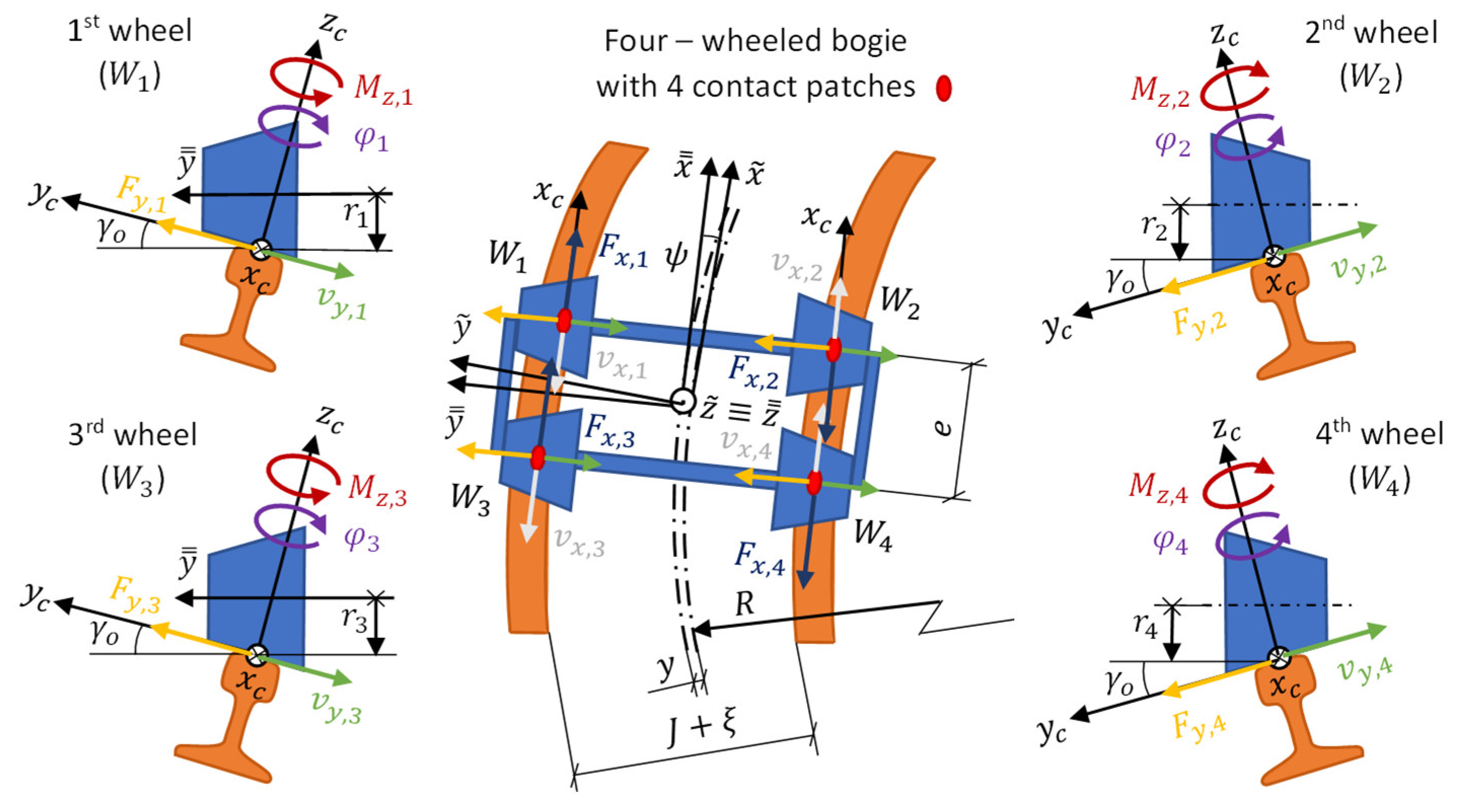
Finally, Figure 7 shows the tangential forces and torques associated with the creepages at each wheel of a four-wheeled bogie. The main dynamics equations are introduced thereafter: those for normal force computation on each wheel (Eqs. 18 – 26), those which allow applying Hertz’s solution (Eqs. 27 – 36), those which allow applying Polach’s method (Eqs. 37 – 46) and, finally, those of the center of friction model (Eqs. 47 – 51):
Figure 6.
Tangential forces and torques associated with the creepages at each wheel of a four-wheeled bogie. Source: Own elaboration.
Figure 6.
Tangential forces and torques associated with the creepages at each wheel of a four-wheeled bogie. Source: Own elaboration.
2.4.4. Calculation of Wear and Prediction of RCF
Wear is the damage to the wheels which reduces their useful life drastically. This wear is due to abrasive and adhesive wear and there exist models based on a wear rate which enable obtaining the wear depth and, hence, characterizing the damage (Sichani, 2016). Abrasive wear is due to the relative movement between the wheel and rail surfaces and their roughness, which cause friction and this, in turn, the loss of wheel and rail material. In contrast, adhesive wear is due to plastic deformation and to the cohesive forces appearing between both surfaces (Van der Waals, electrostatic or chemical), which ends up producing a material transfer from one surface to the other (Rovira, 2012).
For wheel wear characterization, Reference (Rovira, 2012) listed the following hypotheses:
- The equations are parametrized for abrasive wear and not for adhesive wear as both phenomena are already included in the resulting wear law if they have been experimentally calibrated.
- The different mathematical tools study the wear on the wheel profile, where the wear estimated at every instant is cumulative.
- Wear is assumed to be regular: the variation of the transversal profile is studied, not pattern formation along the longitudinal (circumferential) direction. Thus, the wear at a certain position and instant is extrapolated to the whole circumference.
- At the contact interface there are not any pollutants. The effect of pollutants is considering by modifying the friction coefficient or introducing new wear laws.
Considering these hypotheses, the models commented upon in references (Rovira, 2012) and (Sichani, 2016) can be applied to wheel wear characterization. In reference (Pellicer & Larrodé, 2021), energy transfer models and the RAK model are collected and assessed and it was determined that the energy transfer using the USFD wear law since its wear law is continuous, so small errors do not lead to great errors in the end.
Moreover, under high axle loads, the stress distribution around the contact patch may cause fatigue cracks on the wheel surface or inside it. For only predicting if RCF is to appear or not, the fatigue index model developed by reference (Dirks, Ekberg & Berg, 2015) and presented in reference (Sichani, 2016) is useful. The fatigue index () is simply the utilized friction term () minus the shakedown limit () and by comparing its value with zero, 3 situations can be observed: if , RCF is not enough for initiating cracks, while if , this is the limit situation and cracks are not initiated yet. However, if , RCF initiates cracks on the surface since the tangential force is elevated.
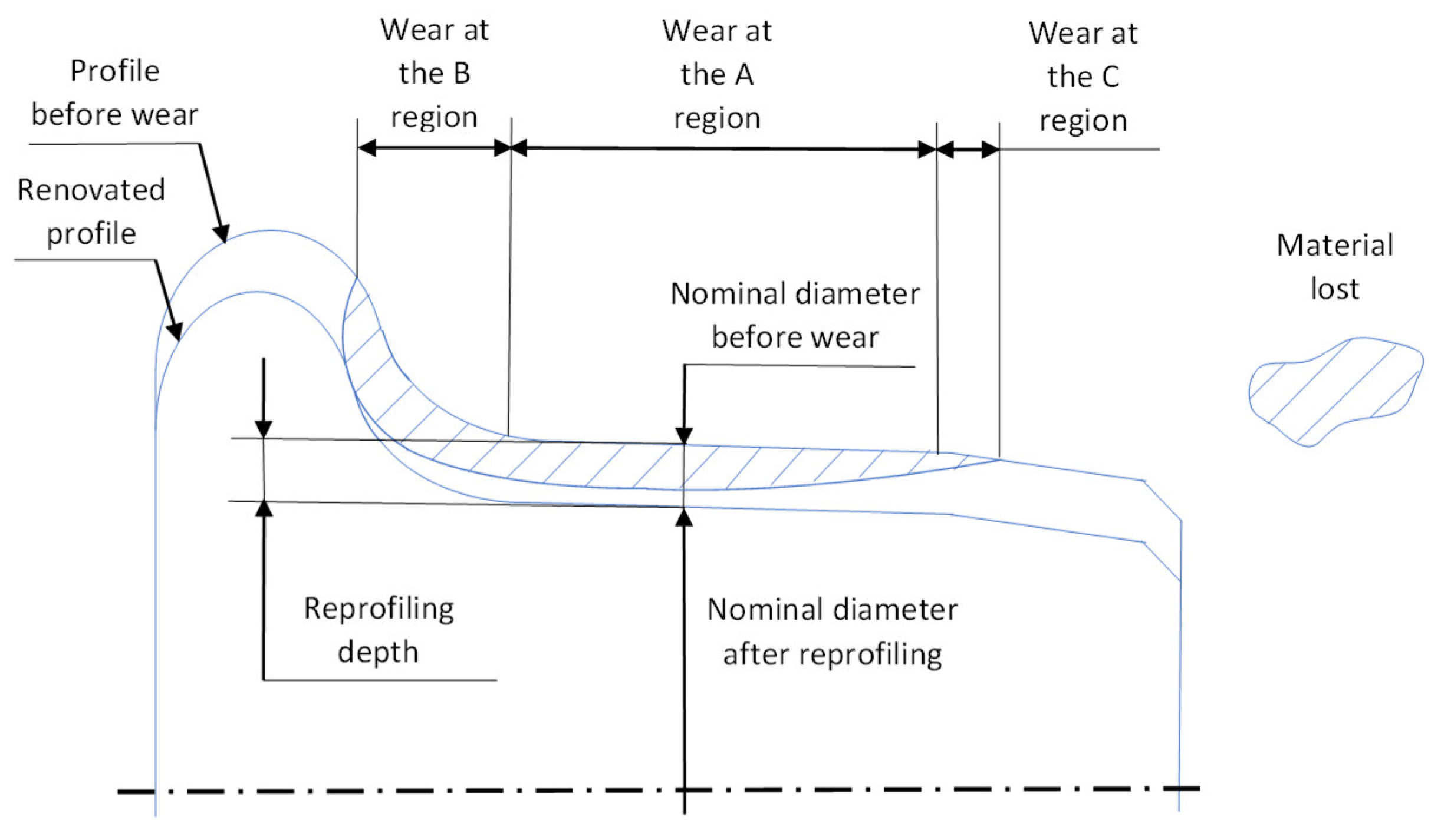
Lastly, Figure 7 shows the wear calculation according to the USFD, which can be eliminated by reprofiling when its depth reaches a certain threshold (Alba, 2015), (Peng et al., 2019), (RENFE, 2020). The main equations of the USFD model are displayed thereafter (Eqs. 52 -56) and the main ones of the fatigue index model (Eqs. 57 – 59) are right next:
Figure 7.
Reprofiling of a wheel which has lost material to wear. Source: Own elaboration.
2.5. Software Choice
Once the algorithm has been defined, it must be implemented in an equation solving program. Due to the large number of input data, equations, relations, functions, procedures and subroutines which had to be implemented, only software capable of processing the entire volume of data in an agile way has been considered. After considering several options (Mathematica, Matlab and Engineering Equation Solver), Engineering Equation Solver (Klein, 1993) has been chosen as it allows building algorithms with any architecture, basing on functions, procedures and subroutines defined in F-Chart programming language, which is a variation of Pascal. The program rearranges internally the equations blocks defined by the user, takes the inputs needed for the new blocks and obtains the requested outputs by means of iterations. These results are obtained after an undetermined number of iterations, depending on adjustable stop criteria such as the relative residuals, which can be as low as 10−10, or the limit of iterations. The specific version used is Engineering Equation Solver Professional V9.457-3D (EES). The chosen program, besides solving algorithms, can create parametric tables and graphs derived from those equations.
2.6. Calculation Scenarios
The objective is to perform a sensitivity analysis of the wheelbase and axle load for low-floor wagons, so as to study their influence on wear. Prior to getting the results, which will be expressed in terms of wheel wear, the calculation scenarios and the input data must be set.
In reference (Pellicer & Larrodé, 2021), many types of bogies are reviewed and, as it can be seen, those bogies with reduced-diameter wheels need more wheels to take up the same load. This is because reduced-diameter wheels can withstand lower axle loads than ordinary-diameter wheels (obviously, smaller wheels have less material), so more wheels are needed for the same bogie load. Also, the minimum diameter after the reprofiling cycles is more restrictive in reduced-diameter wheels for operating safety reasons.
For the sensitivity analysis, these two commercial bogies, used or proposed on rail motorways, have been chosen:
- Y – 25: This bogie consists of four wheels (thus, it is composed of two wheelsets) and it can take up 45 t in total (22.5 t/axle) at a maximum speed of 120 km/h. The nominal wheelbase () is 1.800 m and the wheels are braked, in general, by brake shoes. The wheel nominal diameter () ranges from 920 mm (original, maximum) to 840 mm (operational minimum).
- Graz Pauker 702: This bogie is composed of eight wheels (so four wheelsets) and it can withstand 20 t (5 t/axle) at 100 km/h. The nominal total wheelbase () is 2.700 m (1 + 0.700 + 1 m are the nominal partial wheelbases ()) and the wheel nominal diameter () ranges from 355 to 335 mm.
The sensitivity analysis will be performed for both bogies, for which four calculation scenarios will be established for each (eight scenarios in total, ranging from (a) to (h)). The values chosen for each and every scenario are presented in Table 1:
The rest of conditions are the same (for instance, the rail radii) and are discussed in the Input data section. Only realistic, feasible and plausible values are set and even variations in the geometry and friction are considered (the variation of dry friction with speed).
Taking all of this into account, the eight scenarios are established: Scenario (a) – Scenario (h). For each of them, the input data is entered at first, and then the program runs the algorithm for every stretch of the railway line, switching the direction when the end station is reached. When the wear depth reaches a certain threshold, then the wheel is reprofiled and the scenario execution starts over with a new wheel profile (with a lesser diameter now). After a certain number of reprofiling cycles is reached, the minimum allowed diameter is reached, and the scenario execution ends. All of this is registered in the wheel diameter – mileage curves, which are presented in the Results section.
As for the wear depth threshold, this must be as low as possible for the wheel profiles are not updated as they wear out, so they must be renewed frequently. A sensible value is 1 mm for the three scenarios (this is not an input value, but rather a stop criterion). The lathe will have to remove a bit more for a right reprofiling: 1.5 mm. Converting this radial data into diametral data, 2 and 3 mm are obtained.
Finally, Figure 8 illustrates the placement of the reference frame for the bogies (this reference frame is necessary for the center of friction model), the wheels entering a curve first are shown (wheels and will be half of the times leading and the other half trailing) and the wheel and rail profiles are geometrically adjusted, paying also attention to the flange – rail contact:
2.7. Input Data
As it can be seen in Figure 3, the algorithm needs to input information about the vehicle and the infrastructure before it runs.. The vehicle speed can be linked to the railway line definition if it runs at the maximum allowed speed at the infrastructure.
For the eight scenarios, the wheel profile portrays the geometry of the 1/40 standard profile and is made from ER8 steel grade, while the rail profile portrays the geometry of the 60E1 standard profile and is made from R260 steel grade (AENOR, 2011 – 2021). Most of the wheelset and bogie characteristics, which are taken from the bogie comparison carried out in reference (Pellicer & Larrodé, 2021) are also common to the three scenarios. The same for the parameters used to modify the friction with speed according to Polach’s method (implemented with variable friction under dry conditions). These common input data are shown in Table A3 (Appendix B).
As for the railway line parameters, the calculation is performed for the three scenarios with data from a non-existing railway line. The design parameters of a railway line are defined in references (ADIF, 1983 – 2021) and (Vera, 2016), although not all of the parameters are used for wear calculation.
In reference (Pellicer & Larrodé, 2021), a railway line is defined stretch by stretch, with these parameters:
- Initial and final metric points ( and , respectively).
- Type of stretch: RECTA (straight), CIR (circular curve), CLO (clothoid), PARACUAD (quadratic parabola) or PARACUB (cubic parabola).
- Direction of the curve: NING (the stretch is straight), IZDA (curve to the left) or DCHA (curve to the right).
- Position of the bogie at the curve: NING (the stretch is straight), ENT (the bogie is entering the curve), SAL (the bogie is exiting the curve).
- Curve radius (), cant () and inclination ().
- Initial and final maximum speed allowed ( and , respectively).
Constant values as the track gauge (1.668 m) are the same for all of the stretches, and the gauge widening is a piecewise-defined function which can be directly imported from reference (ADIF, 1983 – 2021), which specifies the gauge widening parameter () as a function of the curve radius (). For example, is null for curves with greater than 300 m and is equal to 20 mm for curves with between 100 and 150 m. Other values as the transition curves parameters are pre-defined and others can be inferred through equations. For instance, the distance traveled between two metric points is their difference.
The 333 stretches defined in reference (Pellicer & Larrodé, 2021) can be found in the supplementary material. The curve radii range from a minimum of 265 m (the ratio is less than 0.01 and according to this heuristic rule, any restricted movements will not appear) to a maximum tending to infinity at straight sections (∞ is not accepted on EES, so it is assimilated to ), with 200 – 800-m radii as the most frequent. For more realism, the station 1 is called Albarque, the station 2 is called Zacarín and there is even an intermediate station called Milbello (all of these are fictional names).
Finally, it is noteworthy that the attached material also includes the polynomial fittings of Hertz’s and Kalker’s coefficients, as well as other equations (displayed making part of the algorithm already) (Pellicer & Larrodé, 2024).
3. Results
3.1. Scenarios for 920-mm Wheels, from (a) to (d)
After executing the algorithm, the diameter – mileage curves are obtained. Here, the diameter is expressed in [mm], whereas the distance traveled is in [km]. The results are discussed in the Discussion section, but some numbers can be anticipated:
- When the 920-mm wheels are mounted on a bogie with m and kg, they can travel for 147,844 km until reaching an 840-mm diameter, losing 2 mm in diameter at every reprofiling cycle. At that point, the worn-out profile will be discarded for safety and operational reasons.
- When the 920-mm wheels are mounted on a bogie with m and kg, they can travel for 98,501 km until reaching an 840-mm diameter, losing 2 mm in diameter at every reprofiling cycle. At that point, the worn-out profile will be discarded for safety and operational reasons.
- If instead the 920-mm wheels are assembled on a bogie with m and kg, they can travel for 134,992 km until reaching an 840-mm diameter.
- Lastly, if the 920-mm wheels are on a bogie with m and kg, they can travel for 83,808 km until reaching an 840-mm diameter.
Figure 9 displays the four diameter – mileage curves. They have been plotted using the same scales on both axes for the sake of visual comparison. As it can be seen, the wheel always starts with a 920-mm nominal diameter (at the tread). Right after reaching the wear depth limit (1 mm in radius or 2 mm in diameter, reached at the flange first), the wheel is sent to the workshop for lathing. This process starts with a diameter close to 920 mm at the tread (barely worn-out) and ends with a 917-mm diameter at the tread. Therefore, 3 mm material are removed (1,5 mm in radius, at each side if looked on a cross-section). The wheel exits the workshop with a 917-mm diameter and it wears out until 915 mm, then it is reprofiled from 917 to 914 mm, and so on:
3.2. Scenarios for 355-mm Wheels, from (e) to (h)
After executing the algorithm, the diameter – mileage curves are obtained. Here, the diameter is expressed in [mm], whereas the distance traveled is in [km]. The results are discussed in the Discussion section, but some numbers can be anticipated:
- When the 355-mm wheels are mounted on a bogie with m and kg, they are able to travel for 60,474 km until reaching their minimum allowed diameter: 335 mm. This is the real life end for this wheel, yet the wear – reprofiling cycles have been extended, as if the final diameter could be 275 mm for the difference between 355 and 275 is the same as that of 920 and 840. In this fictional situation, the wheel would have traveled 221,042 (fictional life end).
- When the 355-mm wheels are mounted on a bogie with m and kg, they are capable of traveling 47,089 km until reaching their minimum allowed diameter: 335 mm. This is the real life end for this wheel, yet the wear – reprofiling cycles have been extended, as if the final diameter could be 275 mm for the different between 355 and 275 is the same as that of 920 and 840. In this fictional situation, the wheel would have traveled 171,116 km (fictional life end).
- If instead the 355-mm wheels are assembled on a bogie with m and kg, then they are capable of traveling 44,699 km until reaching their minimum allowed diameter: 335 mm. In this scenario, the life end could fictionally be 163,382 km (fictional life end).
- Lastly, if the 355-mm wheels are on a bogie with m and kg capable of traveling 25,742 km until reaching their minimum allowed diameter: 335 mm. In this scenario, the life end could fictionally be 94,089 km (fictional life end).
Figure 10 displays the four diameter – mileage curves. They have been plotted using the same scales on both axes for the sake of visual comparison. As it can be seen, the wheel always starts with a 355-mm nominal diameter. Right after reaching the wear depth limit (1 mm in radius or 2 mm in diameter), the wheel is lathed. This process starts with a diameter close to 355 mm at the tread and ends with a 352-mm diameter at the tread. Therefore, 3 mm material are removed. The wheel exits the workshop with a 352-mm diameter and it wears out until 350 mm, so then it is reprofiled from 352 to 349 mm, and so on:
4. Discussion
A model capable of calculating wheel wear has been presented in this work and it has been used to perform a sensitivity analysis by varying influential factors on wear: wheelbase and axle load. For the understanding of these results and the observation of trends, it is necessary to review certain aspects found when analyzing all of the work overall, delving also into the underlying equation blocks which eventually lead to the diameter – mileage curves:
- Scenarios from (a) to (d) can compare to the life of a 920-mm wheel with m and kg: 115,476 km, computed in reference (Pellicer & Larrodé, 2021).
- The 920-mm wheel can operate for 147,844 km in scenario (a), which implies a 28.03 % increase; for 98,501 km in scenario (b), implying a 14.70 % decrease; for 134,992 km in scenario (c), yielding a 16.90 % increase; and, finally, for 83,808 km in scenario (d), so a 27.42 % decrease.
- Scenarios from (e) to (h) can compare to the life of a 355-mm wheel with m and kg: 35,311 km (real life end) and 129,066 km (fictional life end), calculated in reference (Pellicer & Larrodé, 2021).
- Regarding real life ends, the 355-mm wheel can operate for 60,474 km in scenario (e), which implies a 71.26 % increase; for 47,089 km in scenario (f), implying a 33,36 % increase; for 44,699 km in scenario (g), yielding a 26,59 % increase; and, finally, for 25,742 km in scenario (h), so a 27.10 % decrease.
- Regarding fictional life ends, the 355-mm wheel can run for 221,042 km in scenario (e), which implies a 71.26 % increase; for 171,116 km in scenario (f), implying a 32.58 % increase; for 163,382 km in scenario (g), yielding a 26.59 % increase; and, finally, for 94,089 km in scenario (h), so a 27.10 % decrease.
- As it can be seen, increasing axle load is worse than increasing wheelbase (which has an enormous percentual increase). This is because increases in axle load augment both wear depth and the width of the contact patch, whereas increases in wheelbase only augment the former.
- The distance difference between reprofiling (the reprofiling span) is very variable. Should the wagons perform routes Albarque – Zacarín – Albarque (75.272 km) a week, then reprofiling periodicity should be . Because the reprofiling span is not constant inside any of the scenario, the mean value must be computed for everyone.
- According to the reprofiling periodicity criterion, some scenarios are much more unfavorable than others. Scenarios (b), (d) and (h) have a mean reprofiling span below 4,000 km, while in scenario (e) more than 8,000 km are reached. The next bar plot, in Figure 12, displays this information:
- From a maintenance economy perspective, scenarios (e), (f) and (g) are preferrable over (a), (b), (c) and (d), and even scenario (h) is superior to (b) and (d). This means that using Graz Pauker 702 bogies (with 355-mm wheels) with any axle load below 7 t/axle and with a wheelbase equal or less than 1.800 m is better than using Y-25 (with 920-mm wheels) when it comes to maintenance economy.
- In spite of that, Y-25 bogies are commonly used for rail motorways due to its high load capacity. If every wagon incarnates a couple of Y-25 bogies, it will have 4 axles in total, which means that the wagon total load (tare plus payload) will reach 90 t at 22.5 t/axle. By contrast, wagons with a couple Graz Pauker 702 bogies have 8 axles in total, which means that the wagon total load will only reach 40 t at 5 t/axle.
- Comparing the scenarios symmetrically (that is, (a) to (e), (b) to (f), (c) to (g) and (d) to (h)), it can be checked that the fictional life of 355-mm wheels is always higher that the real life of 920-mm ones. The (fictional) life increases, unexpected at first, respond to the different kinematic response of reduced-diameter wheels when negotiating curves. As demonstrated by Redtenbacher’s formula, uncentering is proportional to wheel radius (to wheel diameter in turn, as radius is the half), so not only do reduced-diameter wheels uncenter less than ordinary-diameter ones, but also their flanges will push against the rails less intensely. Moreover, the bogies where reduced-diameter wheels are mounted are less loaded, which will further reduce the force exerted by the rail on the flange (coming from force and torque balances). Figure 13(a) illustrates partial uncentering (differential effect) for the three scenarios and shows how saturation () is reached at a lower radius threshold for reduced-diameter wheels, while Figure 13(b) shows total uncentering (adding bogie rotation) in the worst case (leading wheelset, outer wheel), but even in this case, flange – rail contact is less aggressive owing to dynamics:
- RCF is predicted for every flange – rail contact (except for isolated cases where the 355-mm wheel is negotiating curves with radii close to the threshold radius) as a consequence of the high normal pressure (4 – 5 GPa) at the flange contact area with the rail. This pressure stacks up hydrostatically over a small contact area.
- The effects caused by RCF can be mitigated by setting a reduced wear depth limit (as in the current work). In real operation, the economical factor forces the operators to find the trade-off between crack growth and wear depth limit. Moreover, due to operational safety reasons, their internal regulations forbid eliminating more than 80 mm in diameter for a 920-mm wheel and more than 20 for a 355-mm one.
5. Conclusions
A sensitivity analysis has been carried out and some trends have been observed, all of which have been compared in terms of wheel wear, which is a physical problem affecting railway maintenance economy, and has been tackled through mathematical modeling.
The algorithm constructed interconnects some calculation models and methods by other authors, all of which exhibit good accuracy – computational effort ratios. Moreover, it allows taking into account the main factors impacting wheel wear, some of which are associated with the vehicle (wheel and wagon factors), while others are associated with the superstructure. By introducing boundary conditions and hypothesis complementing those of the calculation models used, the algorithm enables computing the wear with a parametric variation (diameter variation, among others).
In the case presented, wheel wear computations have been utilized for the obtention of diameter – mileage curves for eight scenarios. The main conclusions extracted are:
- Varying axle load has a more acute effect than varying the wheelbase, which can be explained theoretically: Increases in axle load augment both wear depth and the width of the contact patch, whereas increases in wheelbase only augment the former.
- If only maintenance economy is regarded, then Graz Pauker bogies with any load below 7 t/axle and any wheelbase below or equal to 1.800 m is the best option. However, the load capacity is still very limited and Y-25 bogies can carry the double load with half of the wheels. That is why Y-25 bogies are often used in rail motorways.
- Reduced-diameter wheels have a longer life than ordinary-diameter wheels, which can be explained theoretically as well: Regarding kinematics, reduced-diameter wheels negotiate curves more smoothly than ordinary-diameter wheels; while regarding dynamics, their flange – rail contact is softer as well due to less intense uncentering forces and also the fact that the bogie load capacity is lower.
- RCF is predicted for every flange – rail contact, so adopting mitigation strategies will be necessary.
Finally, as a continuation of this research work, a list with the following steps to be carried out is presented:
- Variation of less influential factors in order to develop sensitivity analyses with the goals of tune-fining.
- Reformulation of the algorithm in order to mesh the contact patch and execute calculations globally, including all of the elastic microslips.
- Consideration of conformal contacts, also by means of finite elements as it is not possible to apply Hertz’s solution to this type of contacts.
- Addition of rail wear, which would have an impact on wheel wear as the rail curvatures would change (favorably, in general) and the contact positions would differ.
- Update of the contact parameters immediately after the wheel starts to wear out. This would allow for the computation of the actual semi-conicity, contact angle and radii.
- Inclusion of the wheel and rail surface roughness, which would require a powerful software, able to characterize surfaces with a micrometric resolution.
- Consideration of a different friction coefficient for the tread and flange as it is not always the same, as well as other weather conditions and flange lubrication.
- Study of the effect of brake shoes on the tread. The shoes would tend to increase tread wheel, yet the overall effect is not very pronounced (the shoes wear out first) and the shoes are also helpful for wiping pollutants off of the wheels (for example, leaves).
- Optimization of the maximum wear depth taking into account economic factors: often reprofiling would lower derailment and crack-failure risks; however, that would come at a high cost, so the trade-off point should be optimized.
Author Contributions
Conceptualization, D.S.P. and E.L.; methodology, D.S.P.; software, D.S.P.; validation, D.S.P. and E.L.; formal analysis, D.S.P.; investigation, D.S.P.; resources, D.S.P. and E.L.; data curation, E.L.; writing—original draft preparation, D.S.P.; writing—review and editing, E.L.; visualization, D.S.P.; supervision, E.L.; project administration, E.L.; funding acquisition, E.L. All authors have read and agreed to the published version of the manuscript.
Funding
This research received no external funding.
Data Availability Statement
The data presented in this study are openly available at the MDPI website.
Acknowledgments
This research work is a summary of the Master’s thesis previously completed by the authors.
Conflicts of Interest
The authors declare no conflicts of interest.
Appendix A

Table A1.
Latin-symbol abbreviations.
| Abbreviation | Definition | Unit (SI) | Abbreviation | Definition | Unit (SI) |
|---|---|---|---|---|---|
| Longitudinal semi-axis of Hertz’s ellipse | Degree of the function deceleration - time | ||||
| Lateral acceleration experienced by the vehicle | Number of axles on the vehicle | ||||
| Relative longitudinal curvature | Number of axles on the bogie | ||||
| Hertz’s ellipse area | Lateral Hertz’s coefficient | ||||
| Ratio between the minimum friction coefficient (infinite slip speed) and the maximum (null slip) | Reaction force of the rail on the wheel on the normal contact direction (normal force) | ||||
| Lateral semi-axis of Hertz’s ellipse | Reaction force of the rail on the wheel in the normal direction to the contact area at the (tread flange) at a wheel experiencing flange – rail contact | ||||
| Distance from track center to the rolling radius of the (inner| outer) wheel in relation to the curve | Normal force acting on the (outer| inner) wheel in relation to the curve | ||||
| Distance from track center to rolling radius | Normal force component in the radial |tangential direction (the tangential one is perpendicular to the radial one) | ||||
| Relative lateral curvature | Normal force component acting on the wheel (perpendicularly| tangentially) to contact area | ||||
| Exponential constant at friction law | Existing offset between the track gauge minus the flange – rail play and the distance between the nominal radius center of the wheelset wheels | ||||
| Effective size of contact patch | Horizontal distance between the center of the flange contact area center and the center of the wheel | ||||
| Contact tangential stiffness | Maximum contact normal pressure | ||||
| Contact tangential stiffness for the pure spin case | Initial | final metric point | ||||
| Longitudinal| lateral| vertical Kalker’s coefficient | Theorical rolling radius of the (outer| inner) wheel in relation to the curve | ||||
| Kalker’s coefficient (longitudinal |lateral) corrected according to non-dimensional slip components | Rolling radius of the (outer| inner) wheel in relation to the curve including the displacement due to the yaw angle | ||||
| Kalker’s coefficients on plane | Nominal rolling radius | ||||
| Nominal wheel diameter | Wheel radius measured until the flange contact patch | ||||
| Total bogie wheelbase (measured from its leading to trailing wheelset) | Real rolling radius | ||||
| Partial bogie wheelbase (measured between 2 next wheelsets) | Vertical Hertz’s coefficient | ||||
| Equivalent Young’s modulus of the materials in contact | Curve radius (measured from its center to the track axis) | ||||
| Young’s modulus of the rail | wheel | Rail lateral radius | ||||
| Sagitta of the inner rail in relation to the curve | Wheel lateral radius | ||||
| Magnitude of tangential force vector | Rail longitudinal radius | ||||
| Braking force | Longitudinal wheel radius | ||||
| Traction force | Magnitude of non-dimensional slip vector | ||||
| Longitudinal |lateral tangential force | Longitudinal| lateral non-dimensional slip | ||||
| Longitudinal |lateral tangential force translated to the reference frame | Magnitude of non-dimensional slip corrected with the spin contribution | ||||
| Lateral tangential force (lateral force) corrected with the spin contribution | Lateral non-dimensional slip corrected with the spin contribution | ||||
| Increase in lateral force due to spin | Wear index for the USFD law | ||||
| Maximum tangential force before rolling contact fatigue appears | Coordinate in the axis of the wheel contact area, in the reference frame | ||||
| Fatigue index | Coordinate in the axis of the flange outer part, in the frame | ||||
| Gravity acceleration | Coordinate in the axis of the wheel contact area, in the frame | ||||
| Equivalent shear modulus of the materials in contact | Coordinate in the axis of the flange outer part, in the frame | ||||
| Shear module of the rail | wheel | Longitudinal| lateral creepage | ||||
| Real cant of the railway line | Vehicle speed | ||||
| Center of gravity of height over the rolling plane | Final |initial vehicle speed | ||||
| Center of gravity of height over the rolling plane | Longitudinal| lateral slip speed | ||||
| Center of gravity of height over the rolling plane | Wheel width | ||||
| Total wheel wear depth (USFD law) | Wear rate (USFD law) | ||||
| Railway line gradient / slope | Wheelset uncentering | ||||
| Track gauge | Total wheelset uncentering | ||||
| Wheel semi-conicity or inclination | Available play for the bogie leading wheelset when it uncenters towards the outside of a curve | ||||
| Reduction coefficient for the initial slope of the traction curve at the stick | slip region | Available play for the bogie trailing wheelset when it uncenters towards the inside of a curve | ||||
| Auxiliary coefficient for the calculation of | Wheelset uncentering rate | ||||
| Length really rolled by a wheel | Total wheelset uncentering rate | ||||
| Longitudinal Hertz’s coefficient | Number of wheels on the bogie | ||||
| Spin torque |
Table A2.
Greek-symbol abbreviations.
| Abbreviation | Definition | Unit (SI) | Abbreviation | Definition | Unit (SI) |
|---|---|---|---|---|---|
| Fraction of the force normal to the wheel falling on the flange contact patch | Initial friction coefficient or maximum (null slip speed) | ||||
| Gradient angle | Equivalent Poisson’s ratio of the materials in contact | ||||
| Wheel contact angle | Poisson’s ratio of the rail | wheel | ||||
| Maximum indentation between the two bodies in contact | Gauge widening (at tight curves) | ||||
| Auxiliary coefficient for the obtention of coefficient | Density of the wheel material | ||||
| Tangential stress gradient at the stick region | Longitudinal displacement angle of the contact patch | rad | |||
| Tangential stress gradient at the stick region for the pure spin case | Maximum tangential stress transmitted | ||||
| Load (horizontal| vertical) on the flange contact patch | Tangential yield stress of the wheel material | ||||
| Play between the flange and the rail | Tilt angle | ||||
| Hertz’s angle | rad | Variation angle of tilt angle | |||
| Real cant angle | rad | Spin (rotational creepage) | |||
| Axle load | Yaw angle | ||||
| Vehicle tare | Variation rate of yaw angle | ||||
| Payload transported by the vehicle | Angular slip speed when braking per unit length | ||||
| Dynamic friction coefficient (or adhesion coefficient) |
Appendix B
Table A3.
Input values common to the three scenarios (920 and 355-mm wheels).
| Variable | Value | Variable | Value | Variable | Value |
|---|---|---|---|---|---|
| () | 0.400 | () | 1.235 – 2.747 | () | 1.432 |
| (s/m) | 0.600 | () | 1 | () | 1.432 |
| (m) | 1.800 | () | 0.400 | () | 51 – 70 |
| (Pa) | (m) | (m) | |||
| (Pa) | (m) | (kg) | 20,000 | ||
| (m·s-2) | (m) | () | 0,400 | ||
| (Pa) | (m) | () | 0.550 | ||
| (Pa) | (m) | () | |||
| (m) | 0.512 | (m) | () | ||
| (m) | 1.573 | () | 0 | (kg·m-3) | |
| (m) | (m) | (Pa) | |||
| () | 0.025 | (m) | 0.140 | ||
| () | 0.025 | () | 0.750 |
Notes: (1) Tread’ is the tread of the wheel opposed to the wheel experiencing flange – rail contact. (2) Some values are expressed as ranges since flange – rail contact geometry is a little different at every contact. (3) means that the value tends to infinity (∞ is not accepted on EES).
References
- ADIF. Calificación, geometría, montaje y diseño de la vía. 1983–2021.
- ADIF. Declaración sobre la red. Annual Report. 2023. Available online (in Spanish): https://www.adif.es/sobre-adif/conoce-adif/declaracion-sobre-la-red (accessed on 19 June 2024).
- AENOR. Aplicaciones ferroviarias. Ruedas y carriles. 2011–2021.
- Alba, M. V. Optimización de la Política de Reperfilado de Ruedas para el Citadis 302, en la explotación de Metro Ligero Oeste. Revista Vía Libre Técnica 2015, 9, 29–38. [Google Scholar]
- Andrews, H. I. Railway Traction. The Principles of Mechanical and Electrical Railway Traction, 1st ed.; ElSevier Science: Oxford, 1986. [Google Scholar]
- Corrêa, P.H.A.; Ramos, P.G.; Fernandes, R.; Kurka, P.R.G.; dos Santos, A.A. Effect of primary suspension and friction wedge maintenance parameters on safety and wear of heavy-haul rail vehicles". Wear 2023, 524–525, 204748. [Google Scholar] [CrossRef]
- Cui, D.; Zhang, W.; Tian, G.; Li, L.; Wen, Z.; Jin, X. Designing the key parameters of EMU bogie to reduce side wear of rail. Wear 2016, 366–367, 49–59. [Google Scholar] [CrossRef]
- Dirks, B.; Enblom, R.; Ekberg, A.; Berg, M. The development of a crack propagation model for railway wheels and rails. Fatigue & Fracture of Engineering Materials & Structures 2015, 18, 1478–1491. [Google Scholar]
- European Council. Directive 96/53. Official Journal of the European Communities 1996, L 235/59. [Google Scholar]
- Fissette, P. Railway vehicle dynamics. Teaching content. Catholic University of Louvain, Louvain. 2016. Available online: https://es.scribd.com/document/559372304/RailVehicles (accessed on 19 June 2024).
- Greenwood, J. A. Hertz theory and Carlson elliptic integrals. Journal of the Mechanics and Physics of Solids 2018, 119, 240–249. [Google Scholar] [CrossRef]
- Hertz, H. R. Über die Berührung fester elastische Körper. Journal für die reine und angewandte Mathematik 1882, 92, 156–171. [Google Scholar]
- Jaro, L.; Folgueira, C. A. Las Autopistas ferroviarias: ¿Una apuesta de futuro en líneas mixtas de alta velocidad? Revista de Alta Velocidad 2012, 2, 73–96. [Google Scholar]
- Kalker, J. J. Rolling contact phenomena - linear elasticity, CISM International Centre for Mechanical Sciences, 411th ed.; Springer: Vienna, Austria, 2000. [Google Scholar]
- Klein, S.A. Development and integration of an equation-solving program for engineering thermodynamics courses. Computer Applications in Engineering Education 1993, 1, 265–275. [Google Scholar] [CrossRef]
- Larrodé, E. Ferrocarriles y tracción eléctrica, 1st ed.; Editorial Copy Center: Zaragoza, España, 2007. [Google Scholar]
- Ministerio de Fomento; Ministère de l’Environnement, de l’Énergie et de la Mer. Servicios de Autopista Ferroviaria (AF) en los ejes Atlántico y Mediterráneo. Convocatoria de manifestaciones de interés. Consulta a los fabricantes y diseñadores de material móvil. Report. 2018. Available online (in Spanish): https://www.ecologie.gouv.fr/sites/default/files/180410_AMI_Constructeurs_rapport_ES-min.pdf (accessed on 19 June 2024).
- Ministerio de Fomento. Orden FOM/1630/2015, de 14 de julio, por la que se aprueba la “Instrucción ferroviaria de gálibos”. Boletín Oficial del Estado 2015, 185. [Google Scholar]
- Moody, J. C. Critical Speed Analysis of Railcars and Wheelsets on Curved and Straight Track. Bachelor’s Thesis, Bates College, Lewison, USA, 2014. Available online: https://core.ac.uk/download/pdf/230689735.pdf (accessed on 19 June 2024).
- Oldknow, K. Wheel–Rail Interaction Fundamentals. Course content. 2015. Available online: https://www.coursehero.com/file/185769149/PC-1-3-Wheel-Rail-Interaction-Fundamentals-WRI-2017-20170604pdf/ (accessed on 19 June 2024).
- Ortega, E. Simulación del contacto rueda–carril con Pro/ENGINEER, Bachelor’s Thesis, Universidad Carlos III, Madrid, España, 2012. Available online: https://e-archivo.uc3m.es/entities/publication/1ad42047-7a29-4236-a081-52f4c2ec2646 (accessed on 19 June 2024).
- Pellicer, D. S.; Larrodé, E. Analysis of the rolling phenomenon of a reduced-diameter railway wheel for freight wagons, as a function of operating factors. Master’s Thesis, University of Zaragoza, Zaragoza, Spain, 2021. Available online: https://deposita.unizar.es/record/64448 (accessed on 19 June 2024).
- Pellicer, D. S.; Larrodé, E. Supplementary material of “Sensitivity analysis for low-floor wagons”. Mendeley Data, 1st version, 2024. Available online: https://doi.org/10.17632/8dfxgyvk99.1 (accessed on 19 June 2024). [CrossRef]
- Peng, B.; et al. D. Comparison of wear models for simulation of railway wheel polygonization. Wear 2019, 436 – 437. [Google Scholar] [CrossRef]
- Piotrowski, J.; Chollet, H. Wheel–rail contact models for vehicle system dynamics including multi-point contact. Vehicle System Dynamics 2005, 43, 455–483. [Google Scholar] [CrossRef]
- Polach, O. A Fast Wheel – Rail Forces Calculation Computer Code. Vehicle System Dynamics 2000, 33, 728–739. [Google Scholar] [CrossRef]
- Polach, O. Creep forces in simulations of traction vehicles running on adhesion limit. Wear 2005, 258, 992–1000. [Google Scholar] [CrossRef]
- RENFE. Temario específico para las pruebas presenciales de la Especialidad Máquinas – Herramientas. Material de studio. 2020. Available online: https://www.renfe.com/content/dam/renfe/es/Grupo-Empresa/Talento-y-personas/Empleo/2024/ingenier%C3%ADa-y-mantenimiento/04.%20IYM%20Manual_%20Especialidad_Maquinas_Herramientasv2.pdf (accessed on 19 June 2024).
- Rovira, A. Modelado del contacto rueda-carril para aplicaciones de simulación de vehículos ferroviarios y estimación del desgaste en el rango de baja frecuencia. PhD Thesis, Polytechnical University of Valencia, Valencia, Spain, 2012. Available online: https://riunet.upv.es/handle/10251/14671 (accessed on 19 June 2024).
- Sang, H.; Zeng, J.; Qi, Y.; Mu, J.; Gan, F. Study on wheel wear mechanism of high-speed train in accelerating conditions. Wear 2023, 516–517, 204597. [Google Scholar] [CrossRef]
- Santamaría, J.; Vadillo, E. G.; Gómez, J. Influence of creep forces on the risk of derailment of railway vehicles. Vehicle System Dynamics 2009, 47, 721–752. [Google Scholar] [CrossRef]
- Seo, J.-W.; Hur, H.-M.; Kwon, S.-J. Effect of Mechanical Properties of Rail and Wheel on Wear and Rolling Contact Fatigue. Metals. 2022, 12, 630. [Google Scholar] [CrossRef]
- Sichani, M. S. On Efficient Modelling of Wheel – Rail Contact in Vehicle Dynamics Simulation. PhD Thesis, KTH Institute of Technology, Stockholm, 2016. Available online: https://kth.diva-portal.org/smash/record.jsf?dswid=6030 (accessed on 19 June 2024).
- Soleimani, H.; Moavenian, M. Tribological Aspects of Wheel–Rail Contact: A Review of Wear Mechanisms and Effective Factors on Rolling Contact Fatigue. Urban Rail Transit 2017, 3, 227–237. [Google Scholar] [CrossRef]
- Tipler, P. A.; Mosca, G. Physics for Scientists and Engineers Vol. I, 6th ed.; Macmillan Education: London, UK, 2014. [Google Scholar]
- Vera, C. Proyecto Constructivo de una Línea Ferroviaria de Transporte de Mercancías y su Conexión a la Red Principal. Bachelor’s Thesis, University of Seville, Seville, Spain, 2015. Available online: https://idus.us.es/handle/11441/44482 (accessed on 19 June 2024).
- Wang, H.; Han, J.; Su, M.; Wan, S.; Zhang, Z. The relationship between freight transport and economic development: A case study of China. Research in Transportation Economics 2021, 85, 100885. [Google Scholar] [CrossRef]
- Yenealem, H.G.; Redda, D.T.; Mohammedseid, A. Influence of Axle Load on the Wear of Railway Wheel Material. Modelling and Simulation in Engineering 2023, 6730640. [Google Scholar] [CrossRef]
- Zhai, W.; Jin, X.; Wen, Z.; and Zhao, X. Wear Problems of High-Speed Wheel/Rail Systems: Observations, Causes, and Countermeasures in China. ASME. Appl. Mech. Rev. 2020, 72, 060801. [Google Scholar] [CrossRef]
Figure 1.
Rail motorway train ready for articulated vehicles (un)loading. Source: Own elaboration.

Figure 2.
European and Spanish loading gauges and their possible interferences with a rail motorway. Source: Modification of a diagram from (Fomento, 2015).
Figure 2.
European and Spanish loading gauges and their possible interferences with a rail motorway. Source: Modification of a diagram from (Fomento, 2015).
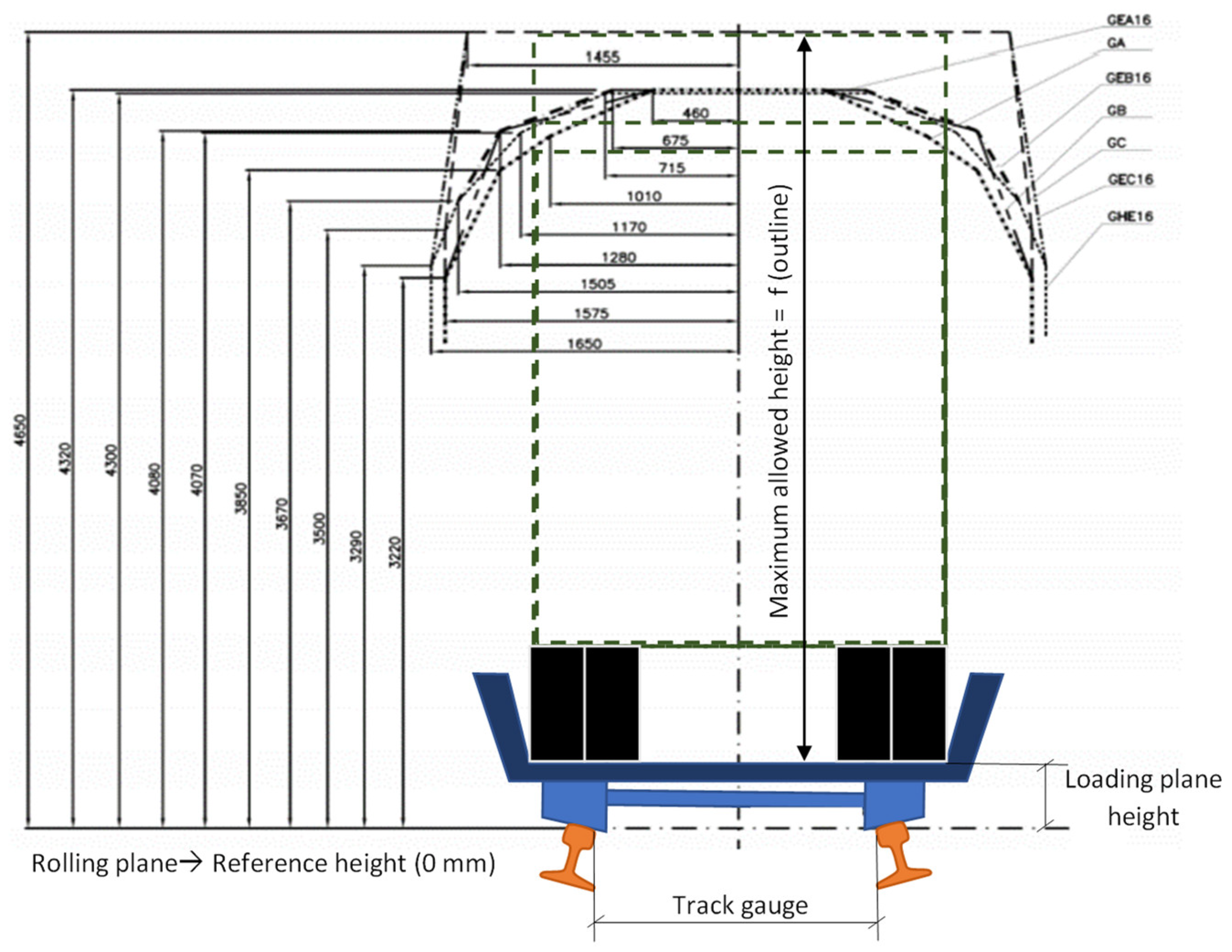
Figure 3.
Flow diagram of the calculation process (algorithm). Source: Own elaboration.
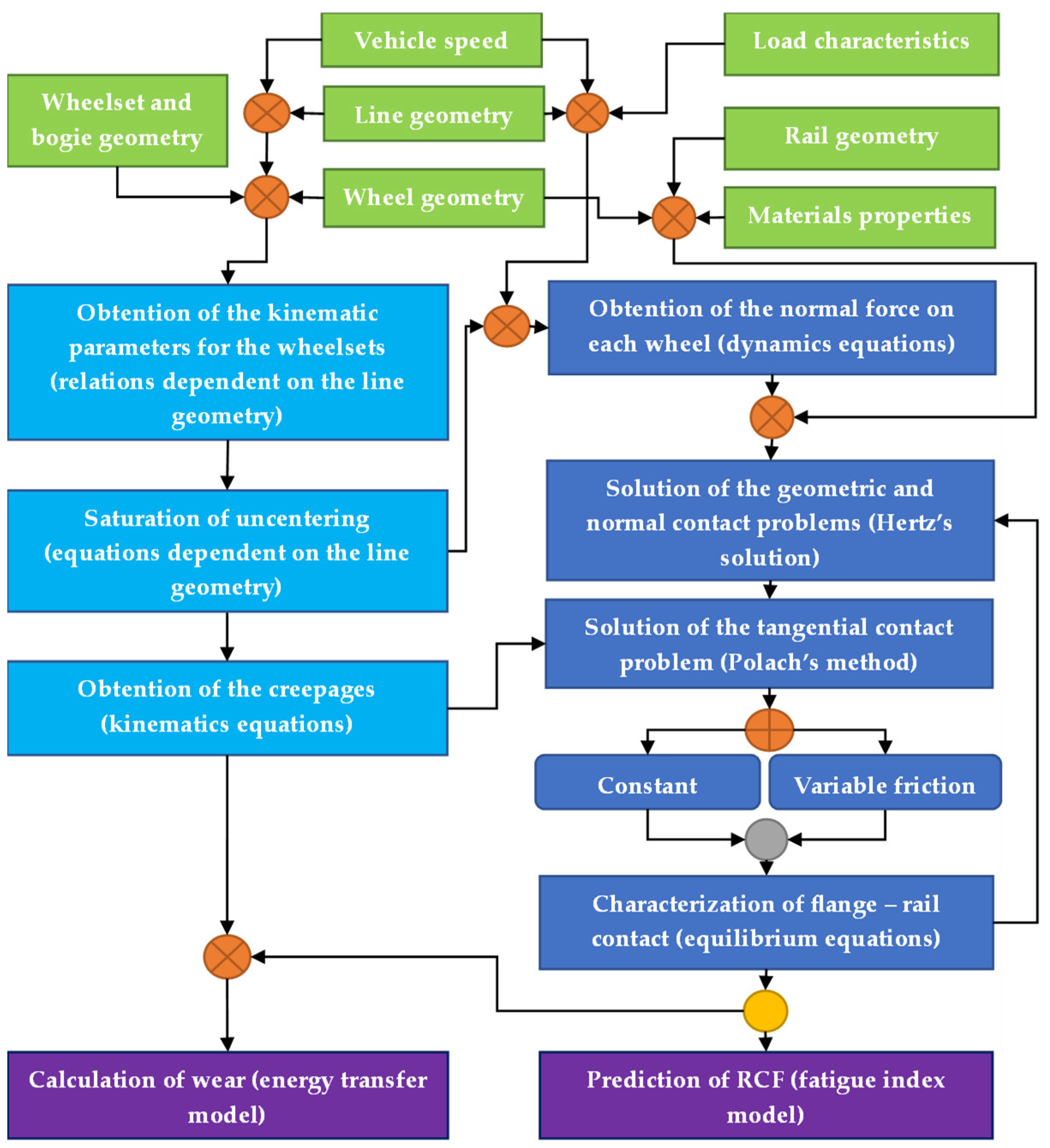
Figure 4.
Reference frames definition. Source: Own elaboration.
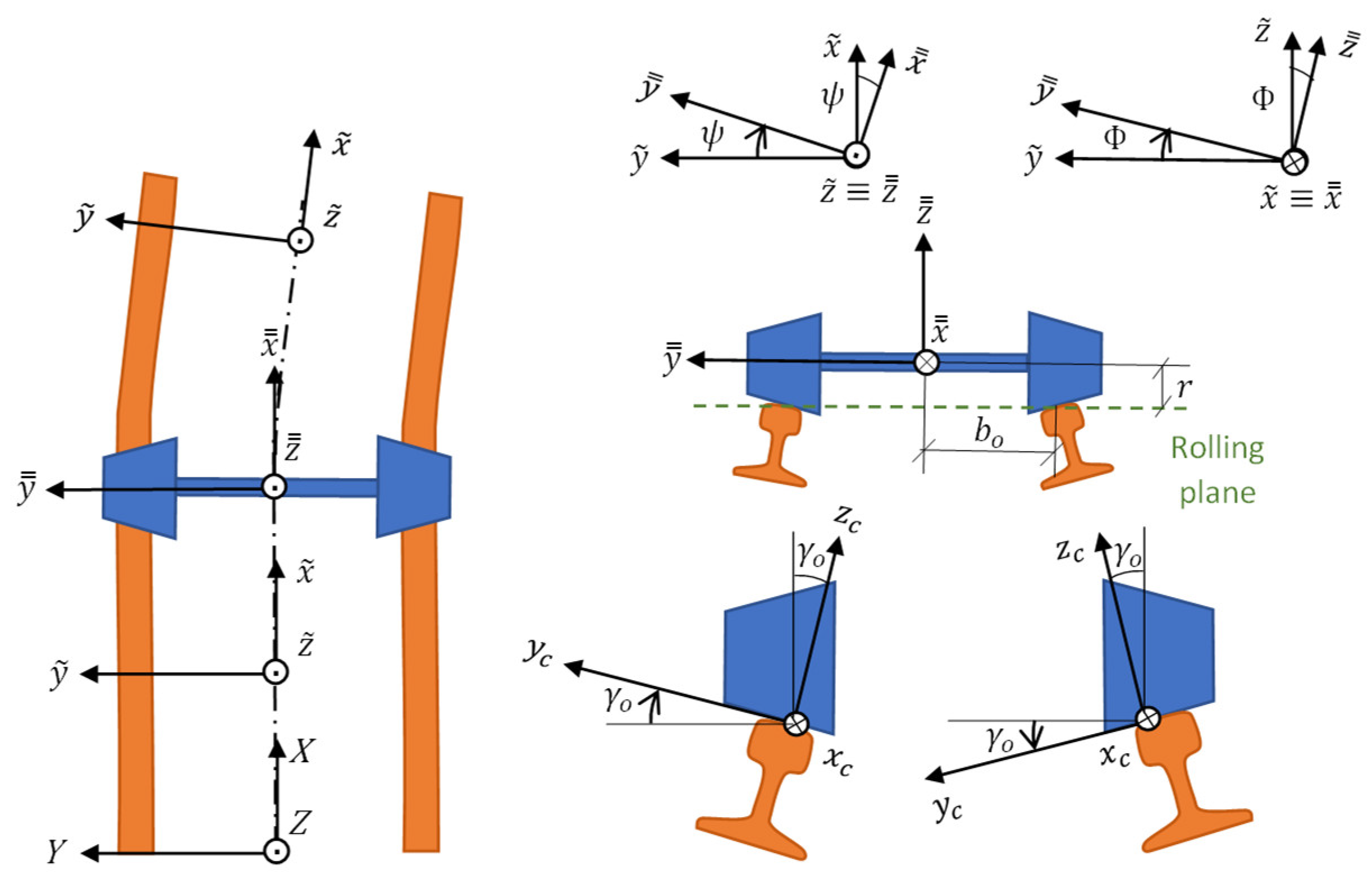
Figure 5.
Wheelset positioning on a narrow curve where there is an uncentering limit imposed by geometrical constraints (for Iberian gauge, mm and , so mm).
Figure 5.
Wheelset positioning on a narrow curve where there is an uncentering limit imposed by geometrical constraints (for Iberian gauge, mm and , so mm).
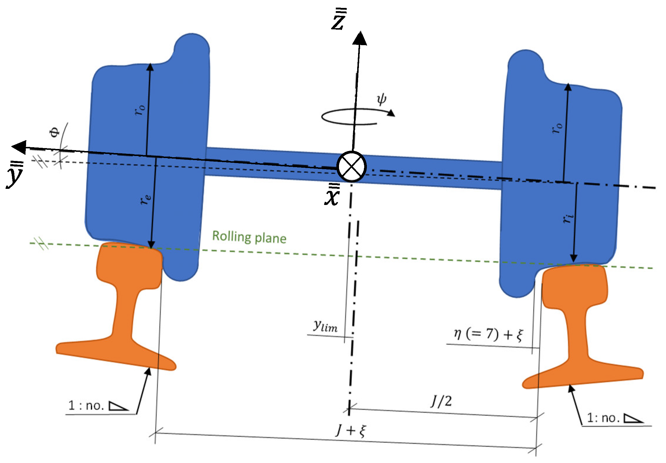
Figure 8.
(a) Placement of the reference frame for the bogies considered; (b) Position of the wheelsets according to the curve direction; (c) Relative positioning of the right wheel and rail at straight sections, with all of the placement dimensions required; (d) Relative positioning of the left wheel and rail at straight sections; (e) Adjustment between the left flange and rail for wear distribution when flange – rail appears. Source: Own elaboration.
Figure 8.
(a) Placement of the reference frame for the bogies considered; (b) Position of the wheelsets according to the curve direction; (c) Relative positioning of the right wheel and rail at straight sections, with all of the placement dimensions required; (d) Relative positioning of the left wheel and rail at straight sections; (e) Adjustment between the left flange and rail for wear distribution when flange – rail appears. Source: Own elaboration.
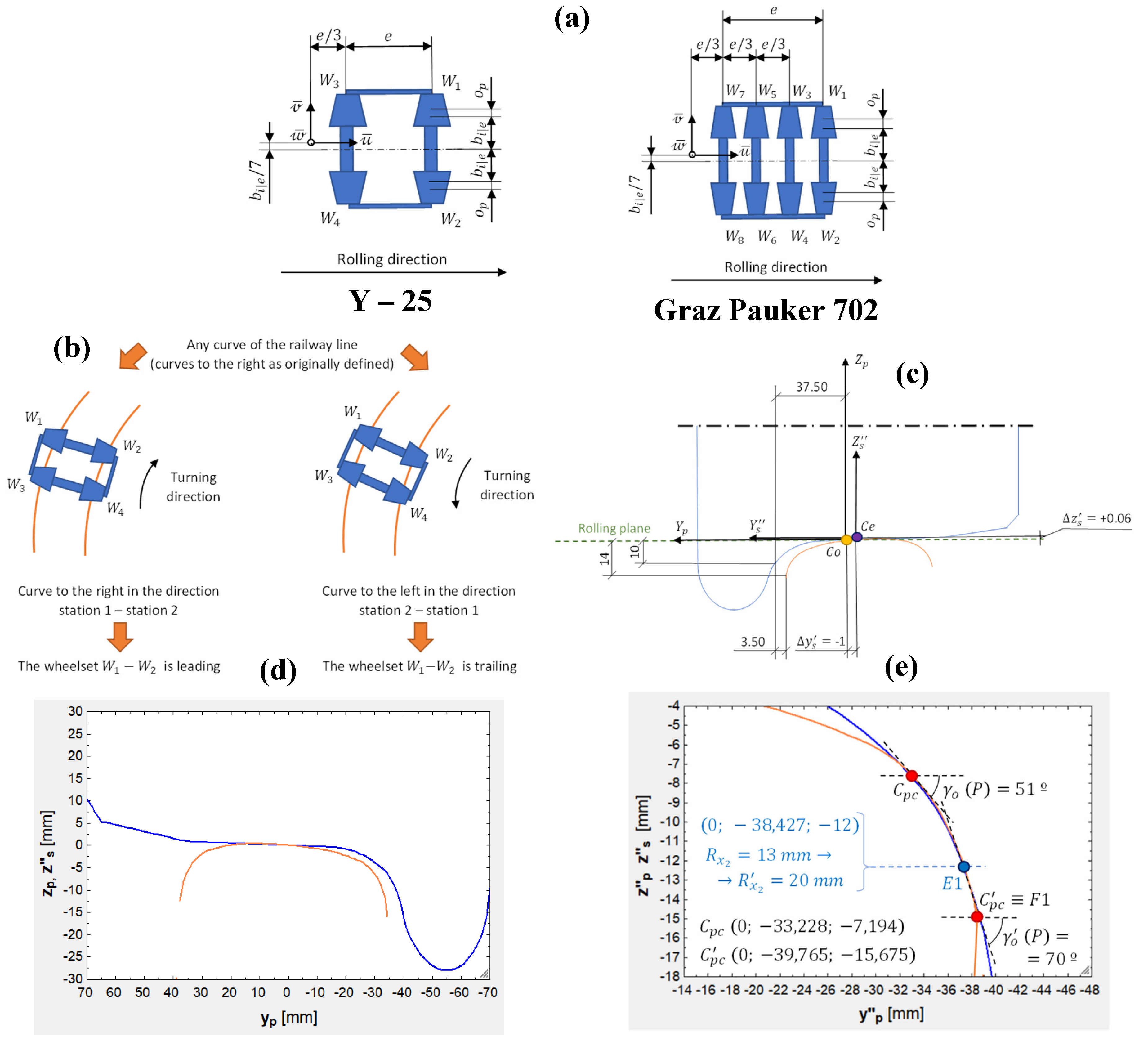
Figure 9.
(a) Diameter – mileage curve for the 920-mm diameter wheel with m and kg; (b) Results for the same wheel, but with m and kg; (c) Results for the same wheel, but with m and kg; (d) Results for the same wheel, but with m and kg.
Figure 9.
(a) Diameter – mileage curve for the 920-mm diameter wheel with m and kg; (b) Results for the same wheel, but with m and kg; (c) Results for the same wheel, but with m and kg; (d) Results for the same wheel, but with m and kg.
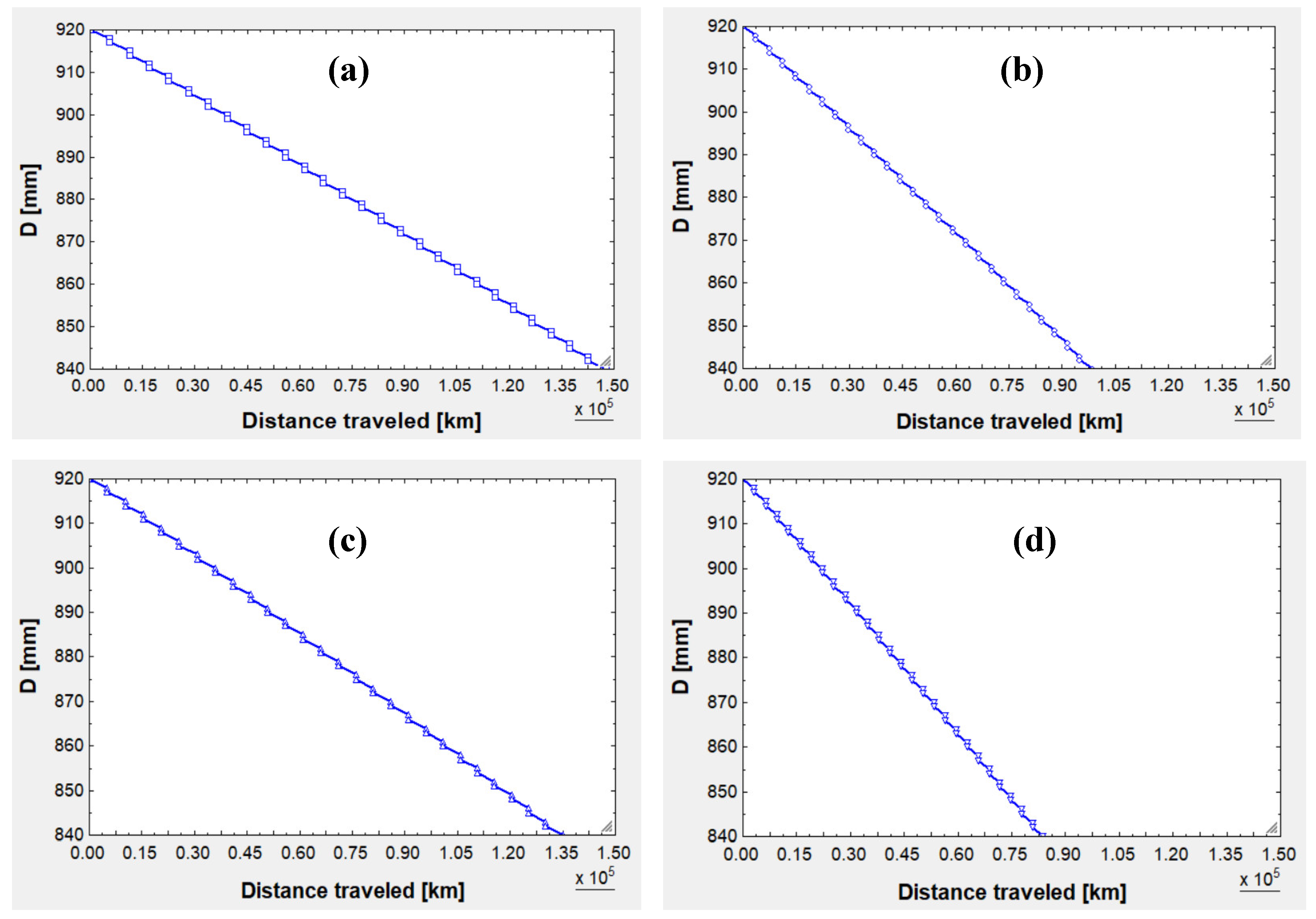
Figure 10.
(e) Diameter – mileage curve for the 355-mm diameter wheel with m and kg; (f) Results for the same wheel, but with m and kg; (g) Results for the same wheel, but with m and kg; (h) Results for the same wheel, but with m and kg.
Figure 10.
(e) Diameter – mileage curve for the 355-mm diameter wheel with m and kg; (f) Results for the same wheel, but with m and kg; (g) Results for the same wheel, but with m and kg; (h) Results for the same wheel, but with m and kg.
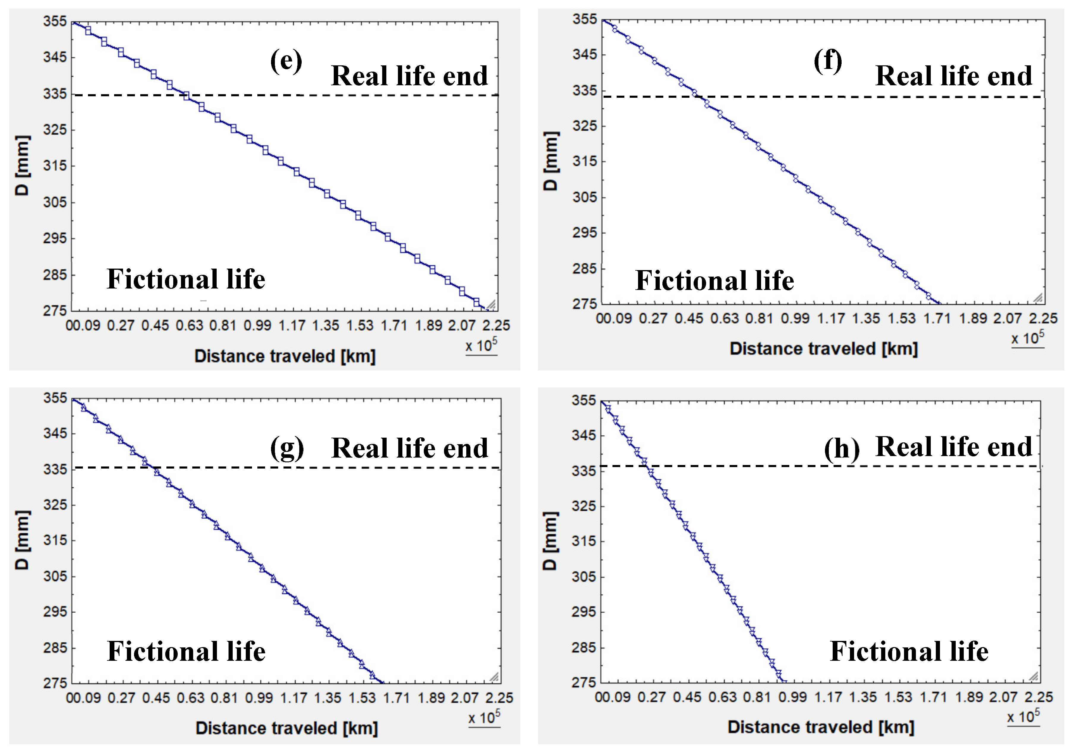
Figure 11.
(a) Life variation with axle load for 920 and 355-mm wheels; (b) Life variation with wheelbase for the same wheels.
Figure 11.
(a) Life variation with axle load for 920 and 355-mm wheels; (b) Life variation with wheelbase for the same wheels.
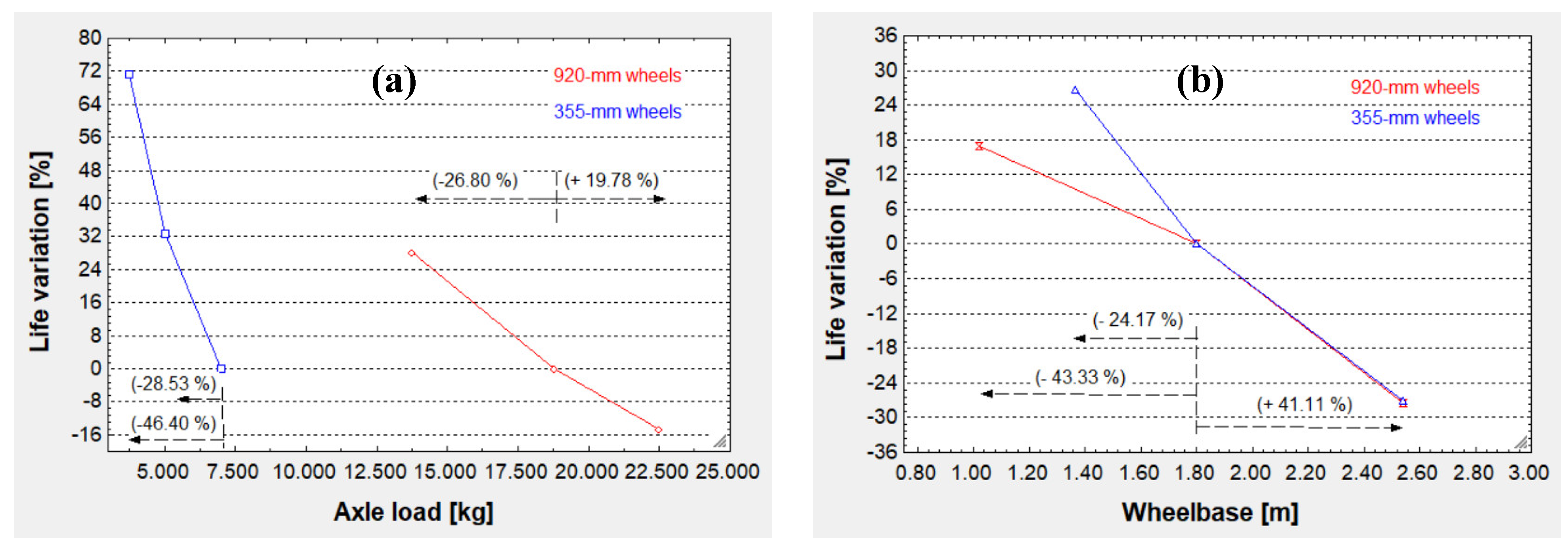
Figure 12.
Mean reprofiling span for each scenario.
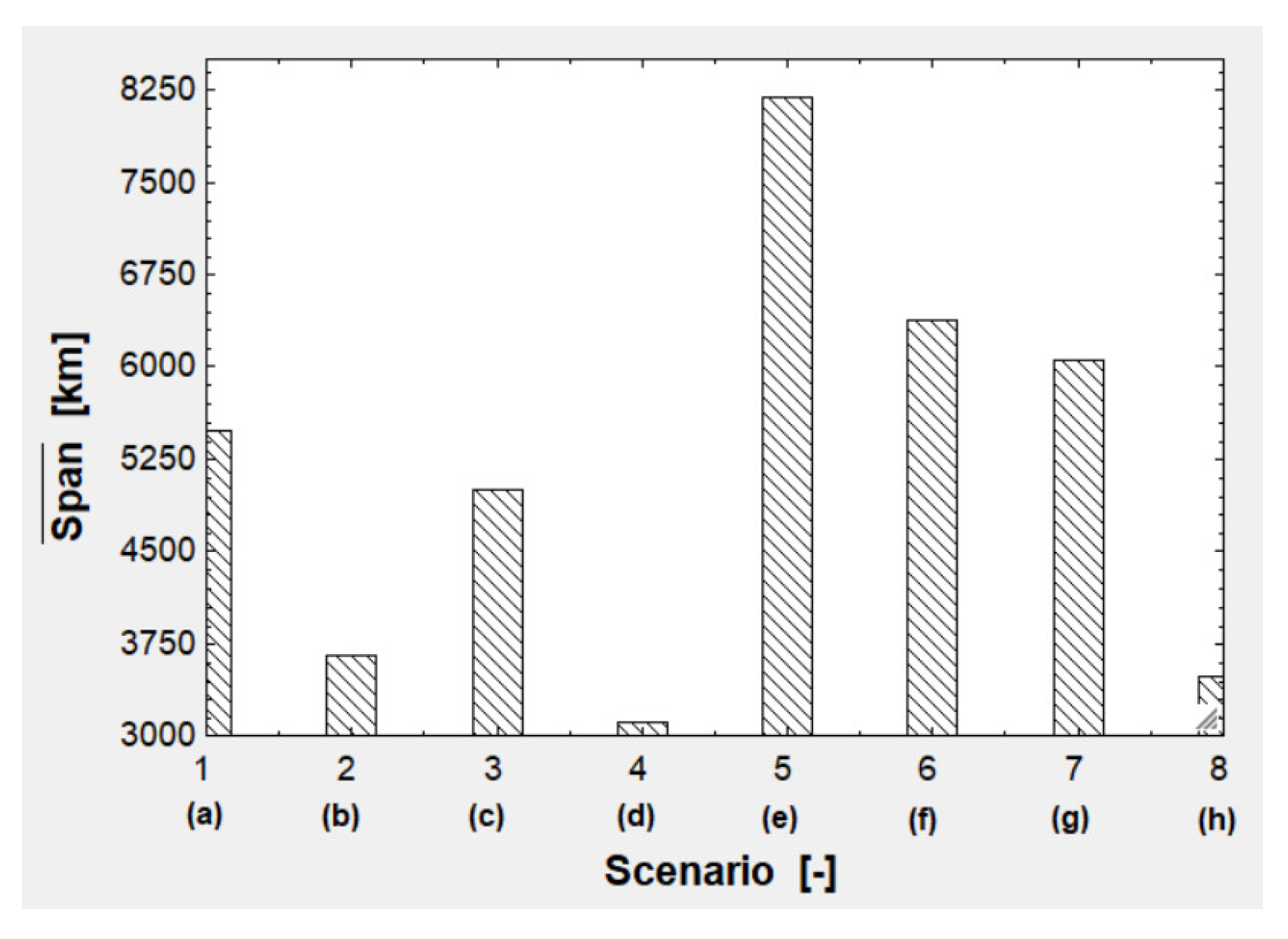
Figure 13.
(a) Partial uncentering for different and values; (b) Total uncentering for the same values, in the worst case (leading wheelset and outer wheel).
Figure 13.
(a) Partial uncentering for different and values; (b) Total uncentering for the same values, in the worst case (leading wheelset and outer wheel).
Table 1.
Specific input values for each of the eight scenarios.
| Variable | (m) | ) | (m) | (m) | (kg) |
|---|---|---|---|---|---|
| (a) | 0.920 | 4 | 0.467 – 0.475 | 1.800 | 13,750 |
| (b) | 0.920 | 4 | 0.467 – 0.475 | 1.800 | 22,500 |
| (c) | 0.920 | 4 | 0.467 – 0.475 | 1.020 | 18,784 |
| (d) | 0.920 | 4 | 0.467 – 0.475 | 2.540 | 18,784 |
| (e) | 0.355 | 8 | 0.185 – 0.193 | 1.800 | 3,750 |
| (f) | 0.355 | 8 | 0.185 – 0.193 | 1.800 | 5,000 |
| (g) | 0.355 | 8 | 0.185 – 0.193 | 1.365 | 6,996 |
| (h) | 0.355 | 8 | 0.185 – 0.193 | 2.540 | 6,996 |
Note: (1) The flange radius () is obtained as the addition of the nominal rolling radius , half of ) and a constant. (2) The total wheelbase () values must be within this range: [, since ensuring that minimum avoids wheel interference and that maximum avoids restricted movement (less than 1 % of the tightest curve radius, as explained in Section 2.7). (3) The axle load values 18,784 kg for 920-mm diameter wheels and 6,996 kg for 355-mm wheels are equivalent in relation with the material quantity: Specifically, both values generate a 1,235 MPa normal pressure, which is a mean pressure value (maximum axle loads usually induce 1,100 – 1,300 MPa on the wheel), even if the load value for the smaller wheel surpasses the manufacturer’s limit. Further details are gathered in reference (Pellicer & Larrodé, 2024).
Disclaimer/Publisher’s Note: The statements, opinions and data contained in all publications are solely those of the individual author(s) and contributor(s) and not of MDPI and/or the editor(s). MDPI and/or the editor(s) disclaim responsibility for any injury to people or property resulting from any ideas, methods, instructions or products referred to in the content. |
© 2024 by the authors. Licensee MDPI, Basel, Switzerland. This article is an open access article distributed under the terms and conditions of the Creative Commons Attribution (CC BY) license (http://creativecommons.org/licenses/by/4.0/).
Copyright: This open access article is published under a Creative Commons CC BY 4.0 license, which permit the free download, distribution, and reuse, provided that the author and preprint are cited in any reuse.


