
Submitted:
06 June 2024
Posted:
10 June 2024
You are already at the latest version
Abstract
We examine the impact of temperature (T) on the Seebeck coefficient S, i.e., the T dependence of S for the single-component molecular conductor Pd(dddt)_2] (dddt = 5,6-dihydro-1,4-dithiin-2,3-dithiolate) with a half-filled band, where the coefficient is obtained from a ratio of the thermal conductivity to the electrical conductivity. The conductor exhibits Dirac electrons with a nodal line, which shows the energy variation around the chemical potential and the density of states (DOS) with a minimum. Using a three-dimensional tight-binding (TB) model in the presence of both impurity and electron--phonon (e--p) scatterings, we study the Seebeck coefficient S_y for the molecular stacking and the most conducting direction. The impact of T on S_y exhibits a sign change, where S_y > 0 with a maximum at high temperatures and S_y < 0 with a minimum at low temperatures. The T dependence of S_y suggests that the contribution from the conduction (valence) band is dominant at low (high) temperatures.The result is examined using a spectral conductivity \sigma_y(\epsilon,T) as a function of the energy $\epsilon$ close to the chemical potential \mu. Further, the Seebeck coefficients for perpendicular directions (x and z) are examined, to show both S_x and S_z being positive and no sign change in contrast to S_y.
Keywords:
Seebeck coefficient
; nodal line semimetal
; single-component molecular conductor
; spectral conductivity
; DOS
; tight-binding model
1. Introduction
Massless Dirac fermions exhibit characteristic properties of electrons, which originate from the energy band with a linear dispersion [1]. The Dirac electron in a bulk system has been found in the following two kinds of molecular conductors [2,3].
One is the organic conductor -(BEDT-TTF)2I3 under pressures [(BEDT-TTF = bis(ethylenedithio) tetrathiafulvalene], in which the Dirac cone is discovered [4,5] using the tight-binding (TB) model with the transfer energy estimated by the extended Hückel method [6,7,8]. The conductor exhibits a zero-gap state (ZGS) with the density of states (DOS), which vanishes linearly at the Fermi energy. The Dirac cone was confirmed by the first-principles DFT calculation. [9]. Further, a two band model [10,11] has been proposed to examine the Dirac electron in the organic conductor. Several properties of the Dirac cone appear in the temperature (T) dependence of physical quantities. The reversal of the sign of the Hall coefficient, which occurs for the chemical potential being equal to the energy of the Dirac point, was proposed theoretically [12] and was also observed experimentally in the Hall conductivity [13]. The conductivity of Dirac electrons has been examined using a two-band model with the conduction and valence bands. The static conductivity at absolute zero temperature remains finite with a universal value, i.e., independent of the magnitude of the impurity scattering owing to a quantum effect [14]. At finite temperatures, the conductivity depends on the magnitude of the impurity scattering, , which is proportional to the inverse of the life-time by the disorder. With increasing temperature, the conductivity increases for [15]. Although a monotonic increase in the conductivity is expected, the measured conductivity (or resistivity) on the above organic conductor shows an almost constant behavior at high temperatures [16,17,18,19,20]. Noting the electron-phonon (e-p) interaction enhances the resistivity of the conventional metal at high temperatures, a nearly constant conductivity at high temperatures is explained by adding an acoustic phonon scattering to a two-band model with the Dirac cone [21].
Another Dirac electron system has been found in a single-component molecular conductor, [Pd(dddt)2], (dddt = 5,6-dihydro-1,4-dithiin-2,3-dithiolate) [3] which exhibits a three-dimensional Dirac electron system under a high pressure with almost temperature independent resistivity [22]. First-principles calculations [23] show a three-dimensional Dirac electron system, consisting of HOMO (Highest Occupied Molecular Orbital) and LUMO (Lowest Unoccupied Molecular Orbital) bands, and a TB model exhibits a loop of Dirac points [24]. This system is one of systems, called as a nodal line semimetal, i.e., a loop of Dirac points [25,26,27]. There are several studies on the effective Hamiltonian, where a general two-band model is introduced [28] and the explicit calculation is performed for the nodal line semimetal [29]. The conductivity was also examined [30] to comprehend the almost temperature independent conductivity. Recently a TB model was improved using the crystal structure, which was obtained under high pressure [31]. This band calculation shows the DOS, which depends linearly in a wide region of the energy being compatible with the temperature corresponding to almost constant conductivity. Thus, we recalculated the almost constant resistivity in [Pd(dddt)2] using the newly found TB model and by taking account of both impurity and acoustic phonon scatterings [32]. It was shown that an interplay of two kinds of scattering explains the T dependence of the resistivity obtained by the experiment. In addition to two-dimensional systems with Dirac points, three-dimensional system with nodal line semimetal is of interest due to anisotropic conductivity and a common feature of the almost constant conductivity.
Seebeck coefficient, which is proportional to a ratio of the thermal conductivity to the electrical conductivity, is a quantity displaying a competition between the conduction and valence bands in Dirac electrons. It does not depend on details of the e–p interaction and impurity scattering. The general formula has been established in terms of linear response theory [33,34,35]. For the Seebeck coefficient, ( x and y) of the organic conductor -(BEDT-TTF)2I3, there are experiments on the T dependence under hydrostatic pressures , [36,37] where the sign of (perpendicular to the molecular stacking axis) is positive except for low temperatures depending on samples. There are theoretical studies for at ambient pressure with a correlation [38] and for under a uniaxial pressure [39] Using a TB model, [40] which has been derived from the DFT calculation with the experimental lattice structure, it has been shown that the Seebeck coefficient under hydrostatic pressures is positive, i.e., at finite temperatures. However, the Seebeck coefficient of the nodal line semimetal has not yet been clarified.
In the present paper, we examine the Seebeck effect of [Pd(dddt)2] in addition to the conductivity, [32] where the T dependence of takes a crucial role. In Section 2, the model and formulation for the Seebeck coefficient of [Pd(dddt)2] with 1/2-filled band are given. The electronic states are examined by calculating the energy band, the nodal line of Dirac points, DOS, and the T dependence of the chemical potential. In Section 3, we present the Seebeck coefficient and the electric conductivity for both directions being parallel and perpendicular to the molecular stacking (y) axis. They are analyzed in terms of the spectral conductivity [39] Section 4 is devoted to summary and discussion.
2. Formulation
2.1. Model
We consider a two-dimensional Dirac electron system given by
Here, denotes a TB model of the single-component molecular conductor consisting of four molecules per unit cell, which is shown below. The second term denotes the harmonic phonon given by with and ℏ =1. The third term is the electron–phonon (e–p) interaction with a coupling constant ,41]
with , which is obtained by the diagonalization of as shown later. The e–p scattering is considered within the same band (i.e., intraband) owing to the energy conservation with , where [10] denotes the averaged velocity of the Dirac cone. The last term of Equation (1), , denotes a normal impurity scattering.
Figure 1 displays the crystal structure of [Pd(dddt)2] [3,24] which consists of four molecules (1, 2, 3, and 4) with HOMO and LUMO per unit cell providing eight molecular orbitals. These molecules are located on two kinds of layers with the x–y plane, where the layer 1 includes molecules 1 and 3, and the layer 2 includes molecules 2 and 4, respectively. The z axis is perpendicular to the x–y plane of the layers 1 and 2 forming a three-dimensional system.
A revised TB model corresponding to Figure 1 has been recently obtained using the crystal structure observed under pressure [31]. There are several kinds of transfer energies between two molecular orbitals, which are listed in Table 1. The interlayer energies in the z direction are given by a (1 and 2 molecules, and 3 and 4 molecules), and c (1 and 4 molecules, and 2 and 3 molecules). The intralayer energies in the x–y plane are given by p (1 and 3 molecules) and q (2 and 4 molecules) and b (along the molecular stacking y axis). Further, these energies are classified by three kinds of transfer energies given by HOMO-HOMO (H), LUMO-LUMO (L), and HOMO-LUMO (HL).
The TB model Hamiltonian in Equation (1) is expressed as
where are transfer energies between nearest-neighbor sites and is a state vector. The spin degree of freedom is discarded. = H1, H2, ⋯, L3, and L4.
Using a Fourier transform with a wave vector , Equation (3) is rewritten as
where , . We take the lattice constant as unity and then in the first Brillouin zone. is 8 × 8 matrix Hamiltonian, where . denotes a Fourier transform of with a complex conjugate relation . , where the corresponds to the molecular staking axis and the lattice constant is taken as unity. Matrix elements are given in the previous work [32]. These energies in the unit of eV are listed in Table 1, where the gap between the energy of HOMO and that of LUMO is taken as 0.696eV to reproduce the energy band of the first principle calculation [24].
The energy band and the wave function , are calculated from
where and
with H1, H2, H3, H4, L1, L2, L3, and L4.
2.2. Dirac Points and DOS
Since the electron close to the chemical potential is relevant for the electron-hole excitation, we consider only and , i.e., the valence and conduction bands for the present calculation. Thus and are replaced by and for the calculation of the transport, while represents not only the Dirac cone but also full dispersion of and in the first Brillouin zone. The present energy bands provide a nodal line, i.e., a loop of the Dirac point , which is obtained from
The chemical potential is determined self-consistently from
where with T being temperature in the unit of eV and . Equation (8) is the condition of the half-filled band due to the HOMO and LUMO bands. denotes a density of states (DOS) per spin and per unit cell, which is given by
where .
2.3. Electric Transport
The conductivity is given by [42]
3. Electronic States
3.1. Energy Band
Figure 2a shows energy bands (j=4 and 5) for the fixed , where (upper band) and (lower band) correspond to the conduction and valence bands, respectively. It is found that and . One-dimensional band is seen along direction. Two bands correspond LUMO and HOMO, which are convex downward and upward respectively. When HOMO-LUMO coupling is absent, there is an intersection due to an overlapping. When HOMO-LUMO coupling is present, the intersection disappears due to a gap except for a Dirac point . LUMO (HOMO) corresponds to (), when LUMO band is larger than HOMO band. The relation is reversed when LUMO band is smaller than HOMO band. Figure 2b shows energy bands (j=4 and 5) on the – plane for the fixed , The Dirac point exists between and , which correspond to HOMO or LUMO in similar to those of Figure 2a. Note that of Figure 2a is smaller than that of Figure 2b.
3.2. Nodal Line and DOS
Figure 3a shows Dirac points in 3D momentum space forming a nodal line, where A (B) on the line corresponds to a minimum (maximum) of the energy and exists on a plane of (). The width of the energy variation along the nodal line is given by . The chemical potential is located between A and B. The energy is symmetric with respect to the point, and . Figure 3b shows DOS as function of , where denotes the chemical potential at T=0. It is found that due to the nodal line, where the energy varies around . There is an asymmetry of with respect to , which shows for , and for [32] The dashed line denotes , which is defined by . Noting that without tilting of the Dirac cone, which is proportional to the inverse of the averaged velocity of the Dirac cone, [42] the velocity of the valence band () is larger than that of the conduction band () except for the momentum around the the nodal line. The inset denotes the T dependence of , which increases slightly for close to the nodal line and decreases with increasing T for being away from the nodal line.
4. Seebeck Coefficients
Since the present salt of [Pd(dddt)2] shows the largest conductivity along the y–axis, we first examine the Seebeck coefficient . Next we examine ( = x and z) with the direction perpendicular to the y-direction. Further, the mutual relation between the conductivity and the Seebeck coefficient is clarified, where both quantities are determined by the spectral conductivity.
4.1. Coefficient for the y-Axis Direction
Figure 4 shows the conductivity and the components as a function of T for some choices of = 0.0003 and 0.0005 with . ( ) corresponds to the valence band (conduction band), which is given by (). However such a correspondence is invalid in a small region of due to the variation of the energy on nodal line. It is found that at low temperatures (), while at high temperatures (). Thus, the contribution from the valence band is larger (smaller) than that from the conduction band at high (low) temperatures. Such a relation can be understood from DOS in Figure 3b, where the average velocity of the Dirac cone of the conduction band is larger (smaller) than that of the valence band for the electron with ( . The component normalized by the total shows a small dependence on (impurity scattering), while the total one decreases clearly by the increase of .
In Figure 5, the Seebeck coefficient ( 0.0003 and 0.0005) is examined with some choices of 1, 2 and 4. It turns out that there is a sign change of around , where at high temperatures takes a maximum and at low temperatures takes a minimum. At high temperatures, decreases with the increase of R due to the effect of the e–p interaction, which is enhanced by the increase of T as seen from Equation (15a). Note that for is almost independent of R. At low temperatures, reduces to zero in the limit of as seen from Equations (21) and (22) [39]. The Seebeck coefficient with is compared with . The increase of reduces implying that the reduction of is larger than that of . The temperature corresponding to the sign change () decreases for increasing R, but remains almost the same for the increase of .
Figure 6 shows the components of the Seebeck coefficients and for with . comes from the conduction band with , which is obtained from LUMO band outside the nodal line and from HOMO band inside the nodal line. comes from the valence band with , which is given by HOMO band outside the nodal line and by LUMO band inside the nodal line The off diagonal component is negligibly small compared with the diagonal components and . The total contribution is shown by the right hand axis, where at low temperatures and at high temperatures and , i.e., the sign change occurs at . The dotted line denotes and is compared with , where their intersection gives .
4.2. Coefficients for the x and z-Axes Directions
Figure 7 shows and for and z. The conductivity with and z is much smaller than due to the large anisotropy of the velocity , since the transfer energy for the y axis is largest due to the molecular stacking direction. Both and show no sign change. The fact that and at high temperatures suggests that the effect of the conductivity is larger than that of the thermal conductivity. At high temperatures, is much larger than and decreases rapidly. Note that takes a minimum at low T and at . Such a minimum suggests that is close to the sign change as discussed later.
Figure 8 shows components of the normalized conductivity with (solid line) and z (dashed line) for = 0.0003 and . The total conductivity is given by ( = ). Quantities and ( and ) correspond to intraband (interband) contribution, where the interband contribution is negligibly small. The difference between (the valence band) and (conduction band) increases by the increase of T. The difference between and is small compared with that between and . Thus, the main contribution for the conductivity is given by the valence band at high temperatures.
Figure 9 shows components of Seebeck coefficient for and z, which are mainly determined by the intraband contributions, i.e., and . The contribution from the valence band has a positive sign and that of the conduction band has a negative sign. The total Seebeck coefficient has a positive sign due to . The difference between and is negligibly small, while is larger than except for low temperatures. The minimum of at in Figure 7 is compatible with a fact that at low temperatures in Figure 9 (the solid line is compared with the dotted line).
4.3. Spectral Conductivity
The Seebeck coefficient is obtained from the spectral conductivity, which is expanded in terms of . From Equations (21) and (22), the Seebeck coefficient is written as
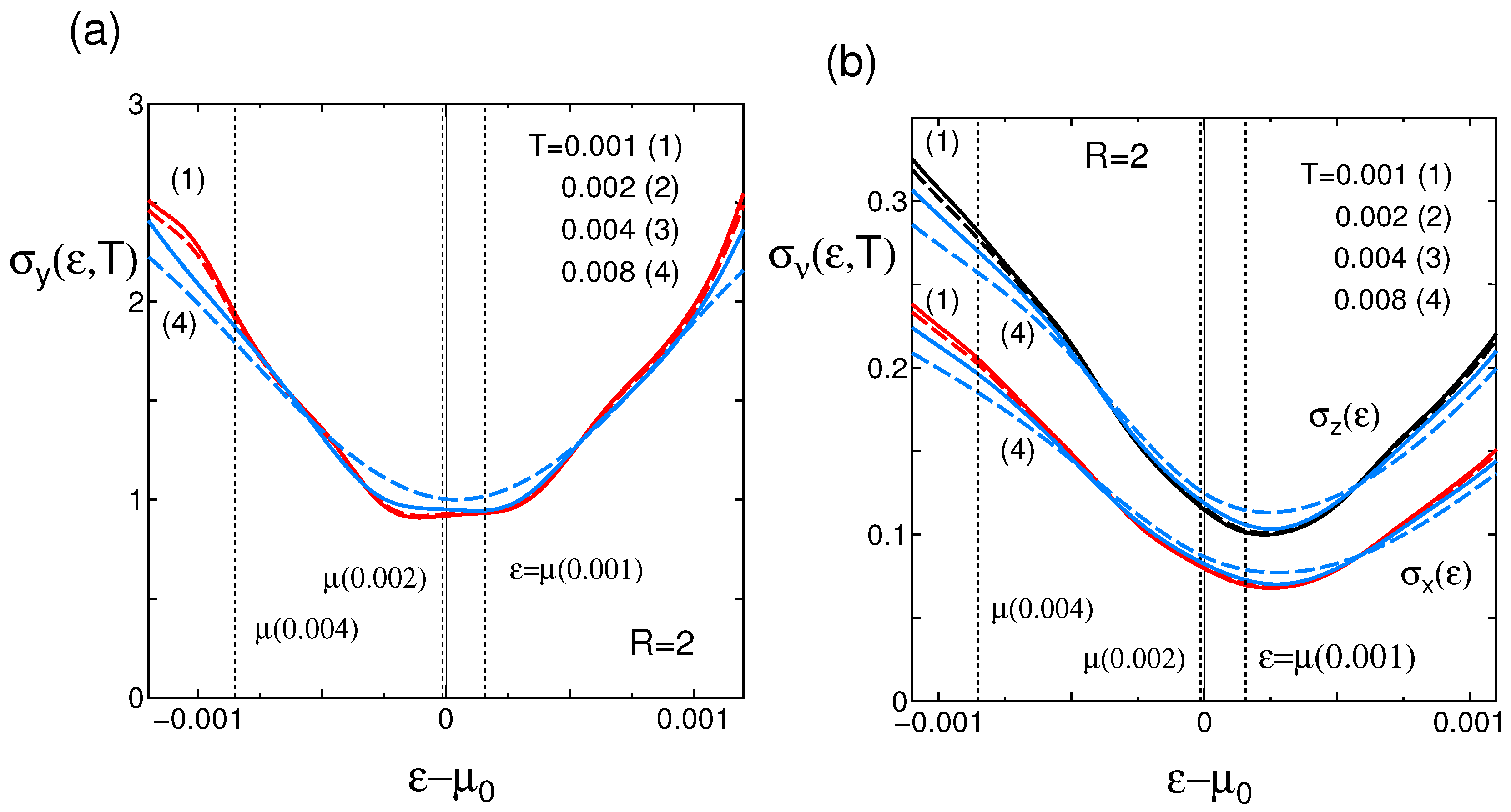
In the limit of low T, the sign of is determined by that of due to . Since the sign change of is determined by zero of the numerator, the temperature for the sign change deviates slightly from that of . In Figure 10a,b, spectral conductivities are shown as a function of .
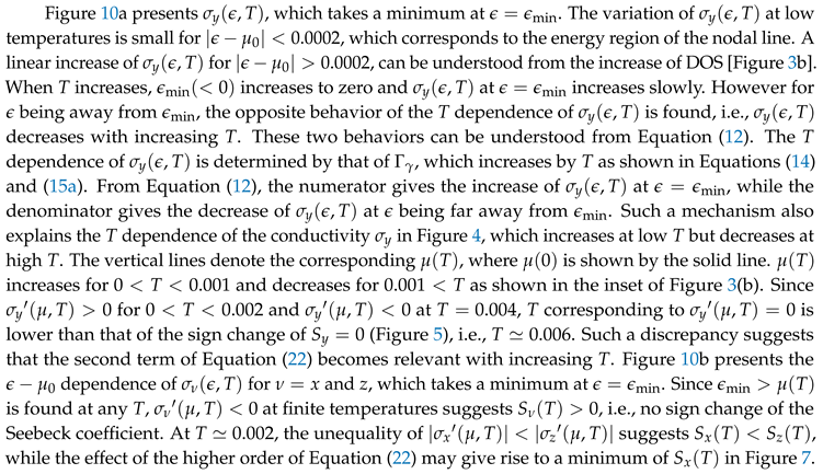
Figure 10.
(Color online) Spectral conductivity as a function of with = 0.0003 and for T = 0.001(1), 0.002 (2), 0.004, and 0.008 (4). The vertical lines denote for the corresponding T. T = 0 and 0.002.
Figure 10.
(Color online) Spectral conductivity as a function of with = 0.0003 and for T = 0.001(1), 0.002 (2), 0.004, and 0.008 (4). The vertical lines denote for the corresponding T. T = 0 and 0.002.
5. Summary and Discussion
In summary, we calculated the T dependence on the Seebeck coefficient ( and z) of the molecular conductor [Pd(dddt)2] under a high pressure and examined in terms of the spectral conductivity . The conductor exhibits the largest conductivity along the y direction corresponding to the molecular stacking, where the z axis is perpendicular to a two-dimensional y–z plane.
Noticeable behavior is found in the T dependence of . With decreasing T, changes the sign from the positive to negative one as seen from Figure 5. This implies the crossover of the dominant contribution from the hole of the valence band () to the electron of the conduction band () (Figure 6). The Seebeck coefficient in Figure 5 is determined by the dependence of the velocity . The sign change is also understood from the energy dependence of DOS being proportional to the inverse of the averaged velocity [Figure 3b], where the average velocity of the conduction (valence) band is larger than that of the valence (conduction) band close to (away from) . This is quantitatively understood from the crossover of the component of the conductivity (Figure 4), where at lower temperatures and at higher temperatures. The result of at low temperature is consistent with the spectral conductivity at low temperature (Figure 10a), i.e., at T = 0.001. Note that such a sign change has been also found for -(BEDT-TTF)2I3 under a uniaxial pressure, [39] which is understood from the components of the conductivity and the spectral conductivity. However, the relevance of the Seebeck coefficient to the asymmetry of the Dirac cone is unclear in the case of the uniaxial pressure.
Finally, we note the T dependence of with and z. There is a large anisotropy of the conductivity, where and are much smaller than suggesting that the velocity for x and z are much smaller than that for y. In this case, it is complicated to discuss the Seebeck coefficient in terms of the dependence of DOS. In fact, there is no change of the sign at low temperatures, i.e., and (Figure 7) implying that the contribution from the valence band is always larger than that from the conduction band (Figure 8 and Figure 9). No sign change at low temperature is also understood from the spectral function, where at low temperatures (Figure 10b). This result shares a common feature with the Seebeck coefficient of the -(BEDT-TTF)2I3 under a hydrostatic pressure, where the hole-like behavior at finite temperatures with the zero doping is obtained [40].
Acknowledgments
The author thanks M. Ogata for useful discussions on the present work.
References
- K. S. Novoselov, A. K. Geim, S. V. Morozov, D. Jiang, M. I. Katsnelson, I. V. Grigorieva, S. V. Dubonos, and A. A. Firsov, Nature 438, 197 (2005).
- K. Kajita, Y. Nishio, N. Tajima, Y. Suzumura, and A. Kobayashi, J. Phys. Soc. Jpn. 83, 072002 (2014).
- R. Kato, H. B. Cui, T. Tsumuraya, T. Miyazaki, and Y. Suzumura, J. Am. Chem. Soc. 139, 1770 (2017).
- S. Katayama, A. Kobayashi, and Y. Suzumura, J. Phys. Soc. Jpn. 75, 054705 (2006).
- A. Kobayashi, S. Katayama, K. Noguchi, and Y. Suzumura, J. Phys. Soc. Jpn. 73, 3135 (2004).
- T. Mori, A. Kobayashi, Y. Sasaki, H. Kobayashi, G. Saito, and H. Inokuchi, Chem. Lett. 13, 957 (1984).
- R. Kondo, S. Kagoshima, and J. Harada, Rev. Sci. Instrum. 76, 093902 (2005).
- R. Kondo, S. Kagoshima, N. Tajima, and R. Kato, J. Phys. Soc. Jpn. 78, 114714 (2009).
- H. Kino and T. Miyazaki, J. Phys. Soc. Jpn. 75, 034704 (2006).
- A. Kobayashi, S. Katayama, Y. Suzumura, and H. Fukuyama, J. Phys. Soc. Jpn. 76, 034711 (2007).
- M. O. Goerbig, J.-N. Fuchs, G. Montambaux, and F. Piéchon,Phys. Rev. B 78, 045415 (2008).
- A. Kobayashi, Y. Suzumura, and H. Fukuyama, J. Phys. Soc. Jpn. 77, 064718 (2008).
- N. Tajima, R.. Kato, S. Sugawara, Y. Nishio, and K. Kajita, Phys. Rev. B 85, 033401 (2012).
- N. H. Shon and T. Ando, J. Phys. Soc. Jpn. 67, 2421 (1998).
- N. M. R. Peres, F. Guinea, and A. H. Castro Neto, Phys. Rev. B 83,125411 (2006).
- K. Kajita, T. Ojiro, H. Fujii, Y. Nishio, H. Kobayashi, A. Kobayashi, and R. Kato, J. Phys. Soc. Jpn. 61, 23 (1992).
- N. Tajima, M. Tamura, Y. Nishio, K. Kajita, and Y. Iye, J. Phys. Soc. Jpn. 69, 543 (2000).
- N. Tajima, A. Ebina-Tajima, M. Tamura, Y. Nishio, and K. Kajita, J. Phys. Soc. Jpn. 71, 1832 (2002).
- N. Tajima, S. Sugawara, M. Tamura, R. Kato, Y. Nishio, and K. Kajita, EPL 80, 47002 (2007).
- D. Liu, K. Ishikawa, R. Takehara, K. Miyagawa, M. Tanuma, and K. Kanoda, Phys. Rev. Lett. 116, 226401 (2016).
- Y. Suzumura and M. Ogata, Phys. Rev. B 98, 161205 (2018).
- H. B. Cui, T. Tsumuraya, Y. Kawasugi, R. Kato R. presented at 17th Int. Conf. High Pressure in Semiconductor Physics (HPSP-17), (2016).
- T. Tsumuraya, H. B. Cui, T. Miyazaki, R. Kato, presented at Meet. Physical Society Japan, (2014).
- R. Kato and Y. Suzumura, J. Phys. Soc. Jpn. 86, 064705 (2017).
- S. Murakami, New J. Phys. 9 356 (2007).
- M. Hirayama, R. Okugawa, S. Murakami, J. Phys. Soc. Jpn. 87, 041002 (2018).
- A. Bernevig, H. Weng, Z. Fang, X. Dai, J. Phys. Soc. Jpn. 2018, 87, 041001 (2018).
- Z. Liu, H. Wang, Z.F. Wang, J. Yang, F. Liu, Phys. Rev. B 97, 155138 (2018).
- T. Tsumuraya, R. Kato, Y. Suzumura, J. Phys. Soc. Jpn. 87, 113701 (2018).
- Y. Suzumura, H. B. Cui, R. Kato, J. Phys. Soc. Jpn. 87, 084702 (2018).
- R. Kato, H. Cui, T. Minamidate, H. H.-M. Yeung, and Y. Suzumura, J. Phys. Soc. Jpn. 89,124706 (2020).
- Y. Suzumura, R. Kato, and M. Ogata, Crystals 10, 862 (2020). see also http://arxiv.org/abs/2009.05272.
- R. Kubo, J. Phys. Soc. Jpn. 12, 570 (1957).
- J. M. Luttinger, Phys. Rev. 135, A1505 (1964).
- M. Ogata and H. Fukuyama, J. Phys. Soc. Jpn. 88, 074703 (2019).
- R. Kitamura, N. Tajima, K. Kajita, R. Reizo, M. Tamura, T. Naito, and Y. Nishio, JPS Conf. Proc..1, 012097 (2014); N. Tajima, private communication.
- T. Konoike, M. Sato, K. Uchida, and T. Osada, J. Phys. Soc. Jpn. 82, 073601 (2013).
- D. Ohki, Y. Omori, and A. Kobayashi. Phys. Rev. B 101, 245201 (2020).
- Y. Suzumura and M. Ogata, Phys. Rev. B 107, 195416 (2023).
- Y. Suzumura, T. Tsumuraya and M. Ogata, J. Phys. Soc. Jpn. 93, 054704 (2024).
- H. Fröhlich, Proc. Phys. Soc. A 223, 296 (1954).
- S. Katayama, A. Kobayashi, and Y. Suzumura, J. Phys. Soc. Jpn. 75, 023708 (2006).
- A. A. Abrikosov, L. P. Gorkov, and I. E. Dzyaloshinskii, Methods of Quantum Field Theory in Statistical Physics (Prentice-Hall, Englewood Cliffs, NJ, 1963).
- M.J. Rice, L. Pietronero, and P. Brüesh, Solid State Commun. 21, 757 (1977).
- H. Gutfreund, C. Hartzstein, and M. Weger Solid State Commun. 36, 647 (1980).
Figure 1.
(Color online) Crystal structure of [Pd(dddt)2] shown in the x–z plane, [24] where the molecule is stacked along the y direction perpendicular to the plane. Layer 1 (molecules 1 and 3) and Layer 2 (molecules 2 and 4) are parallel to the x–y plane and alternated along the z direction. The notations , and z correspond to , and c of the conventional crystallography.
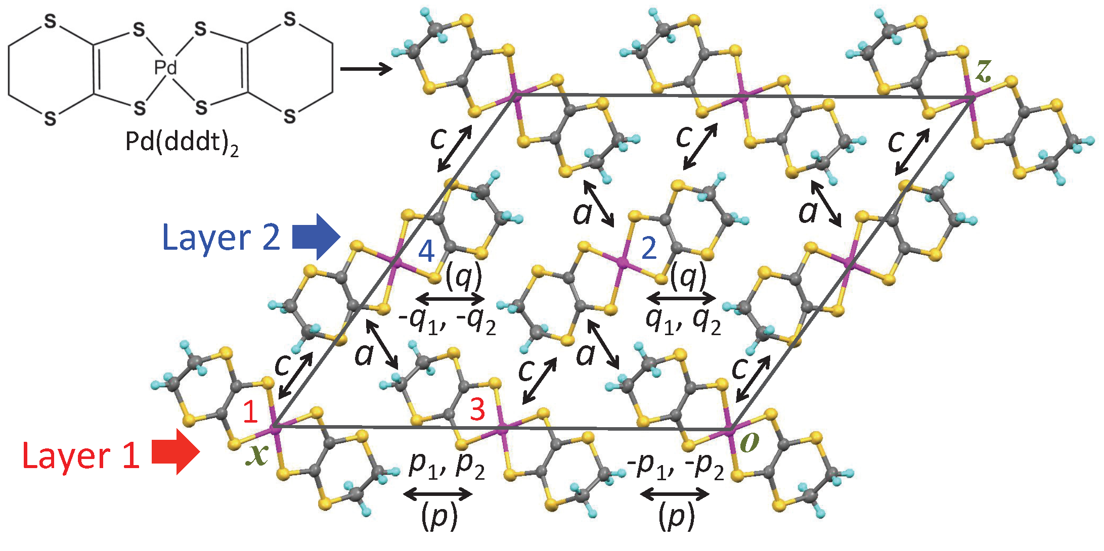
Figure 2.
(Color online) (a) Energy band at where the Dirac point is given by (b) Energy band at where the Dirac point is given by
Figure 2.
(Color online) (a) Energy band at where the Dirac point is given by (b) Energy band at where the Dirac point is given by
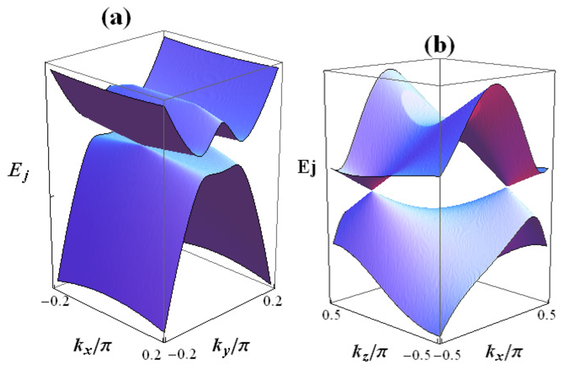
Figure 3.
(Color online) Nodal line (a) and DOS (b) [32] (a) Closed circle denotes Dirac point in 3D momentum space (, , ), which gives a nodal line. The points A and B on the line correspond to a Dirac point in Figure 2a and Figure 2b respectively. They provide a minimum and a maximum of the energy on the nodal line. The chemical potential exists on the line between A and B. (b)DOS [)] is shown as a function of , where denotes the chemical potential at T=0. The dashed line is drawn to compare with the blue line, where the dashed line and the red line is symmetric around . Inset denotes the T dependence of with .
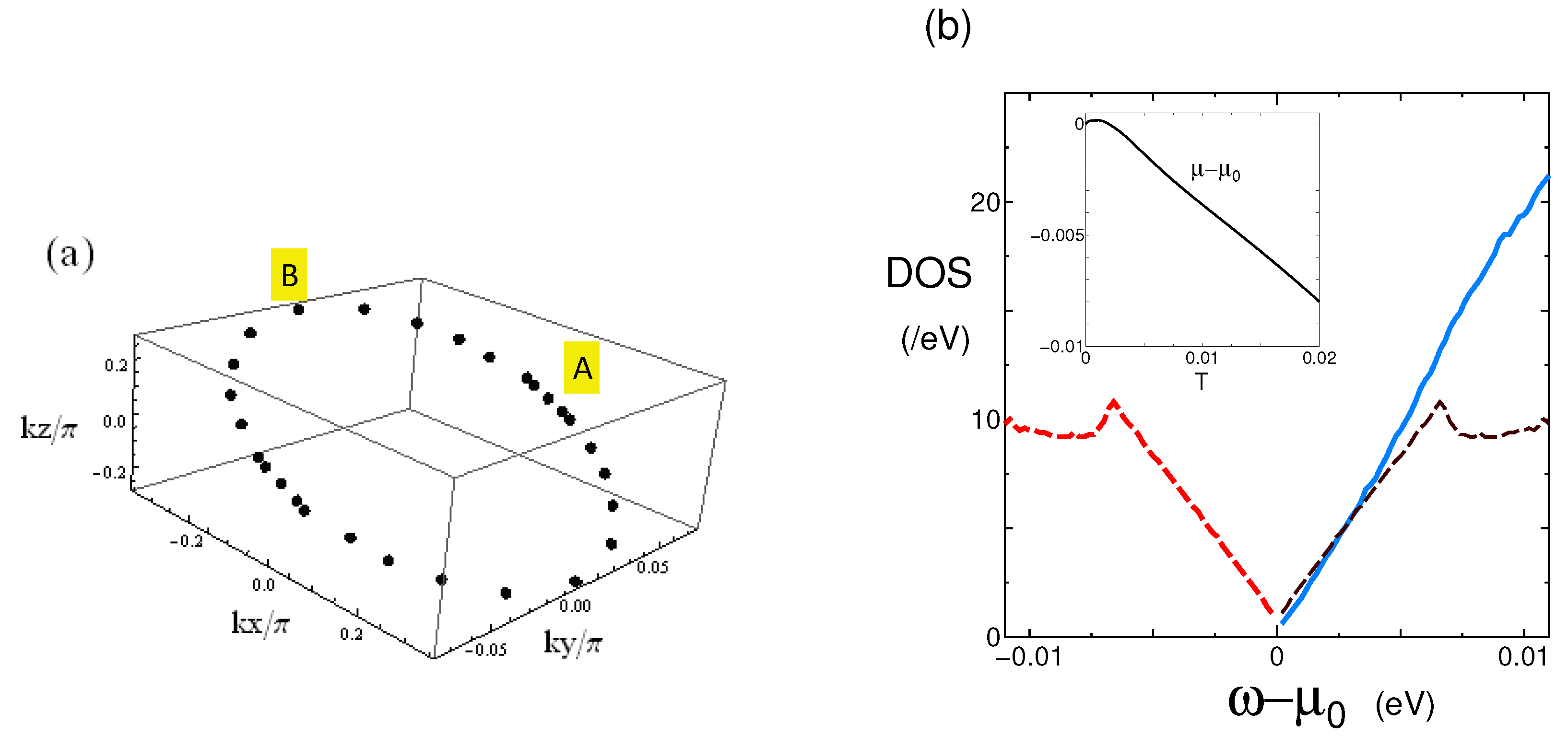
Figure 4.
(Color online) T dependence of the conductivity (right axis) and the components (left axis) for = 0.0003 (solid line) and 0.0005 (dotted line ) with , where . Quantities and ( and ) correspond to intraband (interband) contribution.
Figure 4.
(Color online) T dependence of the conductivity (right axis) and the components (left axis) for = 0.0003 (solid line) and 0.0005 (dotted line ) with , where . Quantities and ( and ) correspond to intraband (interband) contribution.
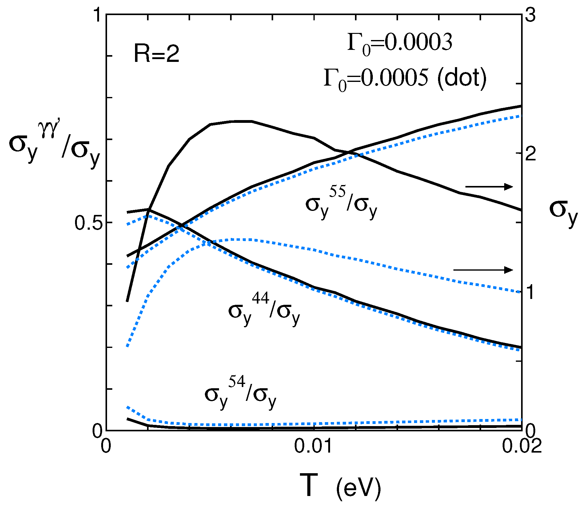
Figure 5.
(Color online) T dependence of the Seebeck coefficient with 1 (dot-dashed line), 2(solid line) and 4(dashed line) for and (dot).
Figure 5.
(Color online) T dependence of the Seebeck coefficient with 1 (dot-dashed line), 2(solid line) and 4(dashed line) for and (dot).
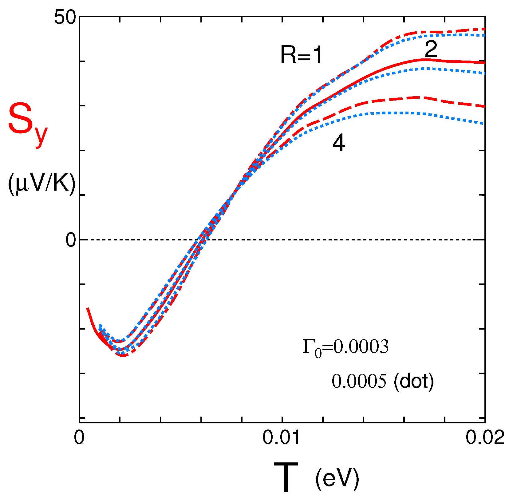
Figure 6.
(Color online) T dependence of the components of the Seebeck coefficients and for with . is negative due to the conduction band with , while is positive due to the valence band with . The interband component is negligibly small compared with the intraband components and . The total contribution is shown by the right hand axis, where at low temperatures and at high temperatures leading to at . The (dotted line) is shown to compare with .
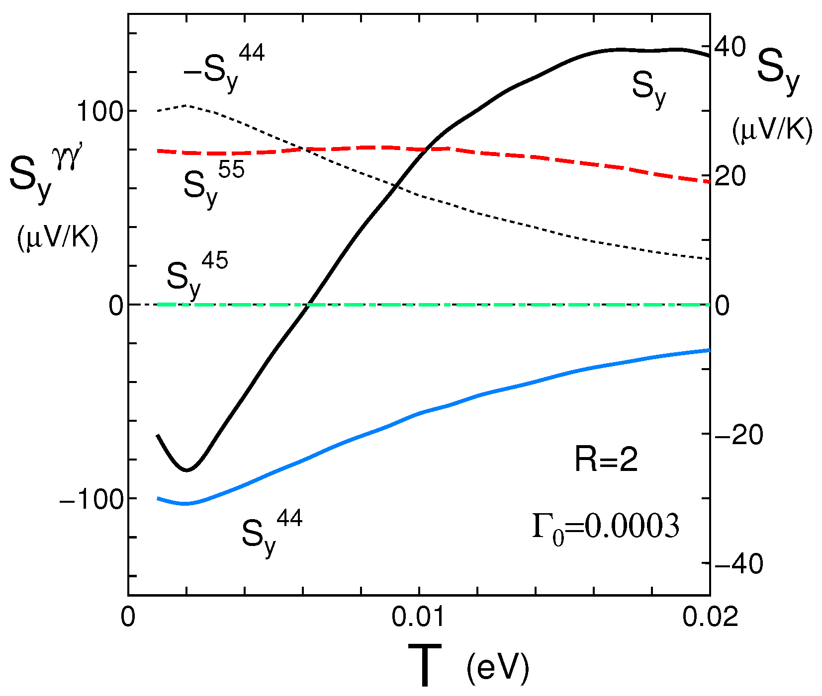
Figure 7.
(Color online) Seebeck coefficient and conductivity for and z with fixed and .
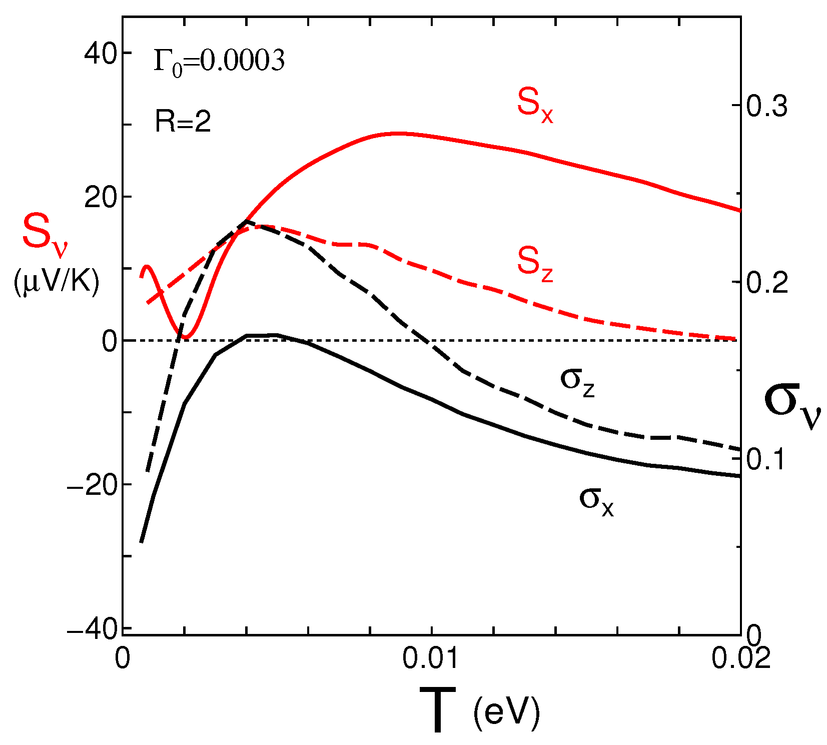
Figure 8.
(Color online) Components of the normalized conductivity with (solid line) and z (dashed line) for = 0.0003 and , where . Quantities and ( and ) correspond to intraband (interband) contribution.
Figure 8.
(Color online) Components of the normalized conductivity with (solid line) and z (dashed line) for = 0.0003 and , where . Quantities and ( and ) correspond to intraband (interband) contribution.
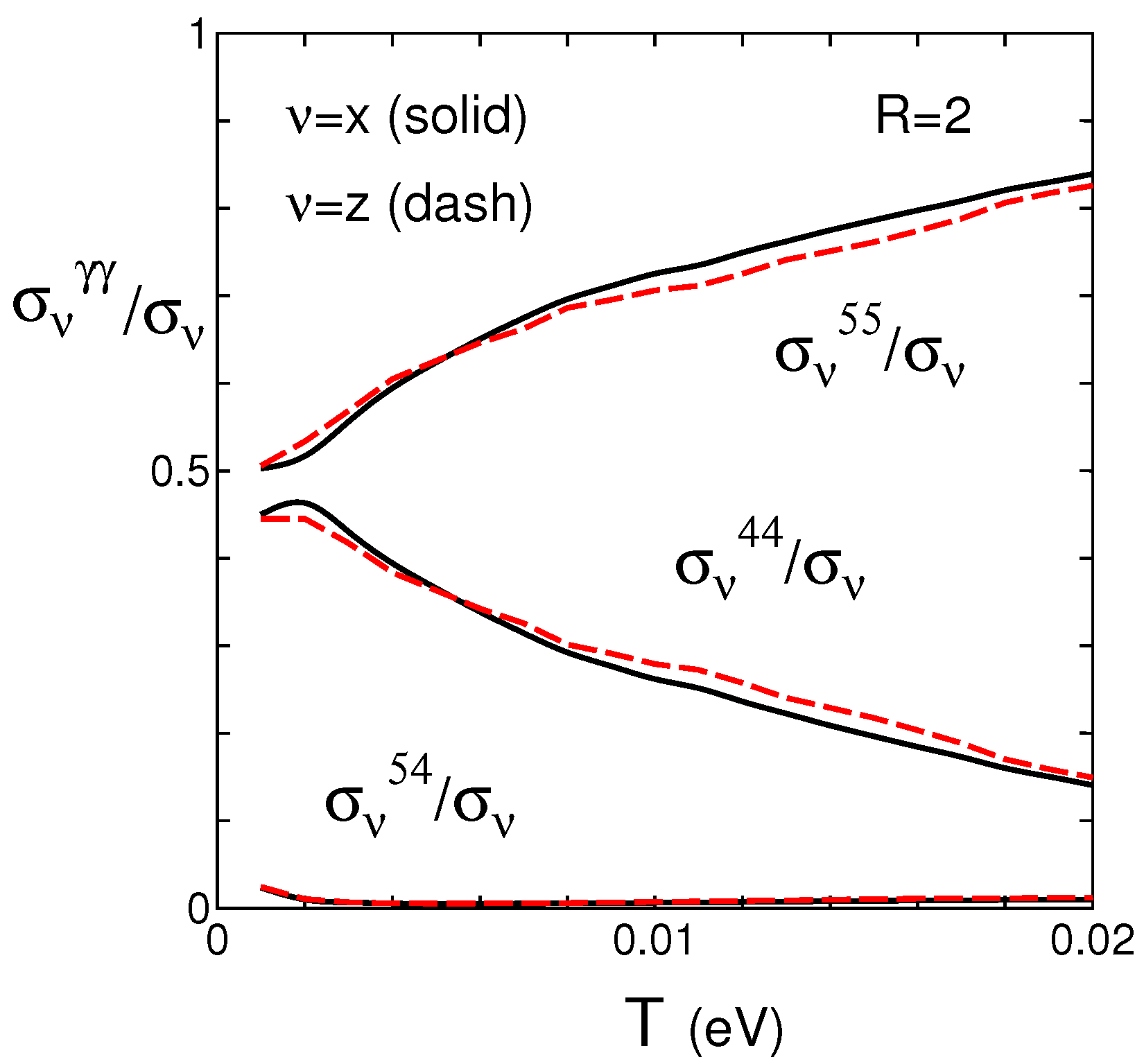
Figure 9.
(Color online) Components of Seebeck coefficient for and z as a function of T.
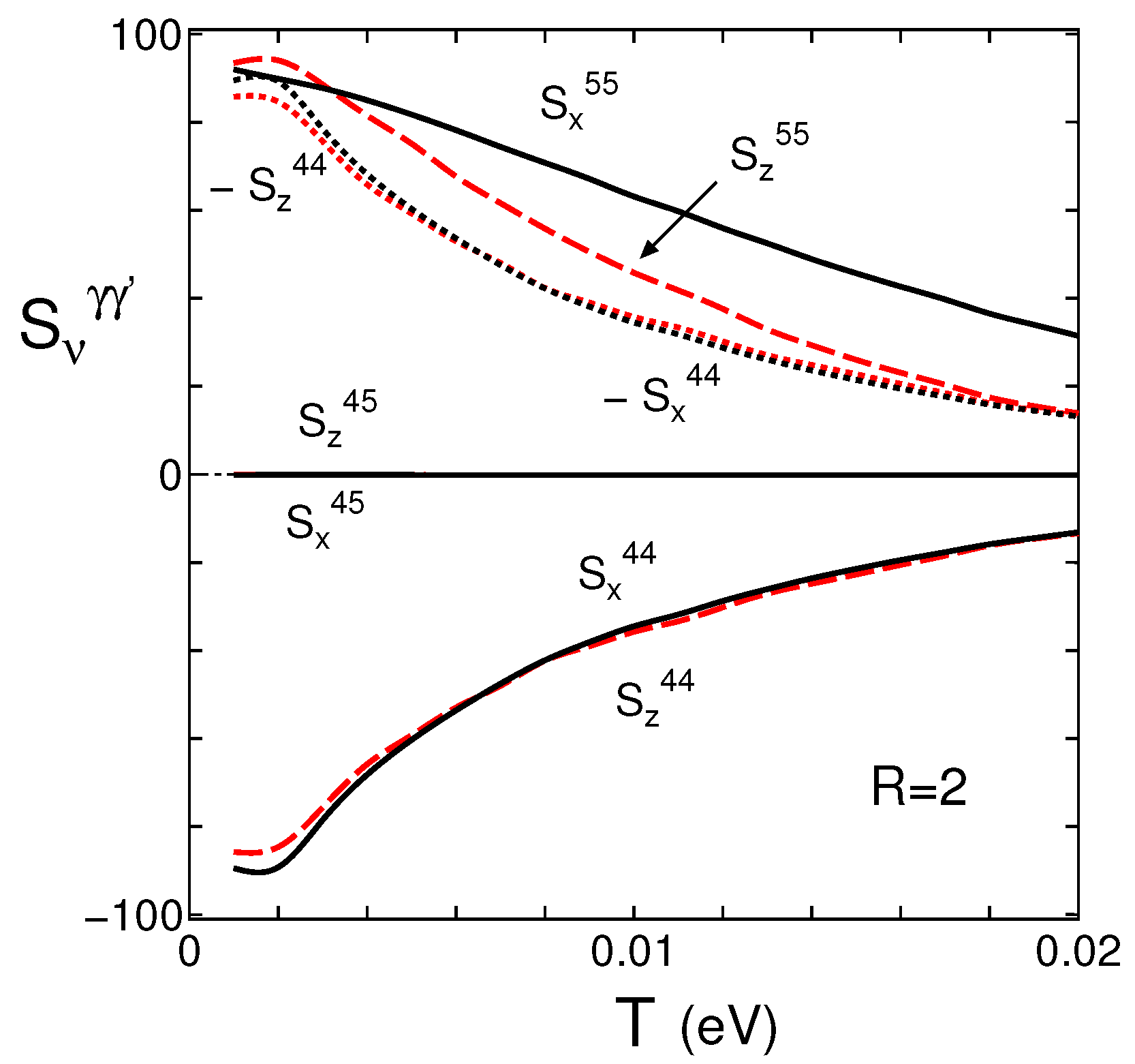

Table 1.
Transfer energies for P=5.9GPa, [31] which are multiplied by eV. The energy difference between the HOMO and LUMO is taken as = 0.696eV.
Table 1.
Transfer energies for P=5.9GPa, [31] which are multiplied by eV. The energy difference between the HOMO and LUMO is taken as = 0.696eV.
| (stacking) | ||||
| Layer 1 | ||||
| — | — | |||
| (stacking) | ||||
| Layer 2 | ||||
| — | — | |||
| Interlayer | ||||
Disclaimer/Publisher’s Note: The statements, opinions and data contained in all publications are solely those of the individual author(s) and contributor(s) and not of MDPI and/or the editor(s). MDPI and/or the editor(s) disclaim responsibility for any injury to people or property resulting from any ideas, methods, instructions or products referred to in the content. |
© 2024 by the authors. Licensee MDPI, Basel, Switzerland. This article is an open access article distributed under the terms and conditions of the Creative Commons Attribution (CC BY) license (http://creativecommons.org/licenses/by/4.0/).
Copyright: This open access article is published under a Creative Commons CC BY 4.0 license, which permit the free download, distribution, and reuse, provided that the author and preprint are cited in any reuse.


