Submitted:
20 October 2025
Posted:
21 October 2025
Read the latest preprint version here
Abstract
We propose that quarks and gluon flux tubes emerge from networks of standing vacuum waves. Each unbound nucleon, in its ground state, may be electromagnetically modeled as massless quantized charge on two pairs of orbiting arcs. Each charge arc is associated with a vacuum fundamental harmonic rotating both poloidally and toroidally. These vacuum fundamental harmonics are coupled to nucleon mass-energy. A mechanism is proposed whereby unbound ground state nucleons continually regenerate their mass and charge. The charge arcs orbit on the two surfaces of a spindle torus with polar charge-exclusion zones. These ground-state models of unbound nucleons may be interpreted as two pairs of virtual Möbius bands. The optimal triangular Möbius band may explain proton uniqueness. These unbound proton and neutron models are shown to be precisely connected via a parameter dependent on neutron mass and the sum of the up and down quark masses during low energy weak interactions. Due to this precise connection, and the relatively high experimental precision of proton magnetic moment, neutron magnetic moment is calculated about two orders of magnitude more precisely than the most accurate experiments to date. This quantum network-based approach to modeling unbound low-energy nucleons calculates several other measurable parameters. This includes utilizing precise lepton vacuum interaction data to develop independent phenomenological proton and neutron vacuum interaction models accurate to 7 digits.
Keywords:
semiclassical
; nucleon g-factor
; Möbius
; fine-structure constant
; quark charge
; quark mass
; weak interaction
; W boson mass
; proton charge radius
; energetic causal sets
; circular Unruh effect
; vacuum interaction
1. Introduction
1.1. Semiclassical Approaches
Recently, semiclassical models of certain physical foundations have been published in high profile journals [1,2,3,4]. These works represent the tip of a growing school of thought. This includes References [5,6], where Yasmineh has recently formulated quantum mechanics in terms of proper time instead of absolute simultaneity. Quantum mechanics formulated in terms of proper time implies that each quantum particle maintains its own internal clock.
In Reference [7], Faber quotes Wheeler’s description of general relativity [8] "Spacetime tells matter how to move; matter tells spacetime how to curve." before adding "Charges and electromagnetic fields tell space how to rotate." This paper combines Faber’s concept with the symmetry of general relativity by proposing that rotating spacetime structures continually regenerate the mass and charge of ground-state protons and neutrons.
Traill has also recently developed rotating spacetime models of some fermions [9]. Traill proposes fermion structures consisting of interfering wavefunctions that form standing waves. Wavefunctions are represented as fields of rotating charge displacement vectors that form spinning spiral wave patterns. Traill applies finite element analysis to these composite wavefunctions. Common to both Traill’s approach and this paper are standing waves, distributed charge, and the absence of singularities.
Several other semiclassical models of quantum particles have very recently been proposed. These include Preziosa proposing a way to connect spacetime curvature and spacetime acceleration [10], Duda proposing a mechanism for the electron and neutrino masses to propel some intrinsic periodic processes [11], and Clarke proposing photon-based quantum particle models involving both poloidal and toroidal electromagnetic circulation [12]. This paper proposes that combined poloidal and toroidal circulations, of standing vacuum waves, are associated with fundamental geometric relationships that yield various properties of unbound low-energy nucleons.
This paper, along with Reference [13], proposes that the charge structure of unbound ground-state nucleons consists of rotating charge arcs with light-speed equators. These charge arcs will manifest as geometrically-simple charge surfaces. Other proposed quantum particle models with geometrically-simple charge surfaces include References [14,15,16]. References [15,16] model charge as the integer U(1) winding number on a thin sheath. Charge sign is determined by the orientation of the phase winding, while charge magnitude is determined by the holonomy count. The dynamics come from minimizing a Maxwell-type action with a holonomy constraint. The core is a topologically protected spin-half standing mode. Finite-size observables are governed by the sheath thickness, rather than the core path length. This proposed quantum particle modeling framework may explain point-like scattering with a narrow near-forward Compton feature. Additional experimental tests are proposed in References [15,16].
This paper assumes that the mass of an unbound ground-state nucleon occupies a completely separate region to its charge structure. Earlier semiclassical particle models have applied similar assumptions. For decades, Rivas has developed particle models based on center-of-mass and center-of-charge separation [17,18,19,20]. This has resulted in one of the few particle models that provides full relativistic equations of motion for the zitterbewegung electron in an electromagnetic field. Rivas’s models apply forces, calculated at the center of charge, to the center of mass. Recently, Fleury has applied Rivas’s electron model to Mott Scattering, which is the spin-dependent deflection of electrons by an atomic nucleus [21]. In Rivas’s electron model, the cycloidal motion of the charge causes scattering asymmetries depending on spin orientation. This can explain why spin-up and spin-down electrons scatter at different angles, which has been experimentally observed at for gold targets [22]. While conventional quantum mechanics explains Moss Scattering with elaborate formalism, Rivas’s model provides an intuitive description of the effect.
1.2. Standard Approaches
Energetic unbound protons and neutrons are extremely complex structures [23,24] that are not fully understood [25,26]. However, at least at low energies, they appear to precisely maintain several important parameters. These include mass, net charge, spin, isospin, parity, magnetic moment, and rms charge radius. While free neutrons spontaneously decay with a mean lifetime of a little under 15 minutes [27], free protons possess such a stable ground state that free-proton decay has never been observed.
Quantum field theory (QFT) is arguably the most successful scientific theory developed to date [28]. It has produced the highly-precise Standard Model of particle physics [29]. However, a considerable number of Standard Model parameters must be experimentally determined. A reason why QFT, sans experiment, may be incapable of precisely explaining the values of certain particle properties could be because operators are applied to create and annihilate particles [28,30]. This conceptual shortcut mathematically precludes potential physical mechanisms that create and annihilate mass and charge.
Center vortices have long been a fixture of nonperturbative quantum chromodynamics (QCD) [31,32]. However, only recently has it been shown how center vortices capture the key nonperturbative aspects of QCD [33,34]. This paper develops a proposal that quantum networks of interfering virtual vacuum momenta continually regenerate the mass and charge of unbound nucleons when in their ground state. These are called unbound ground-state quantum vortex (GSQV) nucleon models. The virtual vacuum momenta in the GSQV nucleon models are standing waves not unlike the center vortices of nonperturbative QCD. Therefore, at energies sufficiently above the ground state, center vortices may emerge from the standing vacuum waves of the unbound GSQV nucleon models.
1.3. Foundational Assumptions Applied in This Work
As with Reference [14], during nucleon-antinucleon pair production, this paper assumes that one real spin-1 photon splits into two virtual circularly-polarized spin-half photon vortices. When in its ground state, each unbound spin-half nucleon’s mass energy is assumed to be continually regenerated from its toroidal vortex component via the combined zitterbewegung and circular Unruh effects [14]. In the GSQV model, the circular polarization of a toroidally revolving virtual photon results in a poloidal vortex component that Reference [14] assumes continually regenerates charge. This paper goes further by mathematically developing a mechanism via which unbound GSQV nucleon charge is continually regenerated via two pairs of vacuum fundamental harmonics rotating both poloidally and toroidally. These rotational dynamics are illustrated by the animation provided at https://youtu.be/nTw6aDd7rRA.
In each unbound GSQV nucleon, the combined toroidal and poloidal actions are proposed to form two pairs of virtual Möbius bands with length set to unbound nucleon Compton wavelength. The width of each virtual Möbius band is set to the nucleon’s vacuum fundamental harmonic length. In an unbound GSQV proton, each virtual Möbius band is proposed to be optimal in the sense of being maximally confined given its length [35,36,37,38]. This maximal confinement is interpreted as a state of minimum energy. By the same metric, an unbound GSQV neutron’s virtual Möbius bands are suboptimal. This may explain why neutron mass energy necessarily exceeds proton mass energy. Other proposed quantum particle models with Möbius geometry include References [15,16,39].
As with the models proposed in References [7,9,11,15,16,40], the unbound GSQV nucleon models are purely field-based and therefore avoid the fundamental dilemmas of point-like particles [30]. This proposed conceptual framework may align with energetic causal set theory–where spacetime emerges from momentum space and the conservation of energy-momentum [41,42,43,44,45,46,47,48].
The modeling presented in this paper is proposed to add to QFT without replacing any of its long-established aspects. The goal is to enhance established QFT by explaining the creation and maintenance of an unbound nucleon’s mass, charge, and magnetic moment while in its ground state. This paper in no way doubts the fundamental validity of QCD [31,32]. Nucleon modeling via lattice QCD may be conceptually correct, but is extremely computationally expensive [49], and it is not known how current quarks transition into dressed constituent quarks [50,51]. The precision of chiral effective field theory (EFT) [52] has generally been good, but recent discrepancies have emerged at the lowest energies [53,54,55,56,57,58]. This paper offers an alternative approach to modeling unbound ground-state nucleons that seamlessly merges with chiral EFT [52] and lattice QCD [49,59] at higher energies.
2. Materials and Methods
All calculations use publicly available CODATA [60] and Particle Data Group [27] data. All calculations were performed using the supplied Excel files, entitled "nucleon calculations" and "Charm quark generating events." All mathematical manipulations were performed by the authors. An animation of intrinsic charm quark generation is provided at https://youtu.be/nTw6aDd7rRA for visualization purposes. The provided GeoGebra file entitled "Proton rotating arcs with charm generation" was used to create the animation and to obtain data for the Excel file entitled "Charm quark generating events."
3. Results
3.1. Nucleon Properties from Quantum Networks
Recently, several semiclassical nucleon models have been proposed [9,12,13,14,15,16,40,61,62,63]. However, References [12] and [61,62,63] propose models that directly conflict with established QCD. In contrast, this paper and References [9,13,14,15,16,40] fully accept established QCD. As with References [13,14], this paper also conceptually explains the origin of quarks, gluons, color charge, and virtual pion clouds. This paper improves the intrinsic charm quark [23,64,65,66,67,68,69,70,71,72,73,74] model proposed in Reference [13].
This paper assumes that any unbound nucleon, in its lowest energy (ground) state, is a completely coherent self-synchronizing structure. At energies above the ground state, these unbound nucleon structures are proposed to transform into the quarks and gluons of established QCD theory. Therefore, at higher energies, there should be no conflict with the established chiral EFT [52] and lattice QCD [49,59] models. The unbound nucleon models developed in this paper may help resolve recently-discovered discrepancies occurring at the lowest energies [53,54,55,56,57,58]. Section 3.1.3 shows that up, charm, and top quark charge appears to depend only on Planck charge, the proportionate area of an unbound GSQV proton’s charge-exclusion zone, and . Section 3.2 applies these quantum network-based models to calculate several parameters related to quarks and neutron decay. The proton models developed in this paper and References [13,14] are statistically consistent with a recent experimental estimate of proton polar charge radius [75].
As with References [13,14], this paper proposes that the properties of an unbound ground-state nucleon’s measured projection can be derived from those of a hypothetical revolving circularly-polarized virtual photon. Such a virtual photon is proposed to propagate via both toroidally and poloidally revolving virtual electromagnetic fields. The virtual photon’s energy is assumed to be identical to nucleon mass energy. The unbound nucleon’s mass energy is proposed to be a quantized manifestation of the circular Unruh energy [76,77,78,79,80,81,82,83,84,85,86,87,88] of an uncharged zitterbewegung fermion [13,14]. It is reasonable to assume that the Unruh effect is fundamentally local [89]. References [13,14] explain mathematically how such an uncharged zitterbewegung fermion could generate a gravitational field by concentrating circular Unruh energy. This results in curved spacetime according to the principles of general relativity [90].
The proposed central uncharged zitterbewegung fermion is shown in Figure 1 of Reference [13]. Following References [13,14], it’s radius is , where is unbound nucleon Compton wavelength. This puts it well inside each massless charge arc described in this paper. This geometry is supported by recent experimental evidence that proton rms mass radius is substantially smaller than proton rms charge radius, and tends to decrease at lower energies [91]. Hansson has argued, that at low momentum transfers, the quarks and gluons of QCD cannot be defined and thus do not really exist within a proton [92]. As with References [13,14], this paper proposes that quarks and gluons do not exist in a nucleon’s absolute ground state, but that gluon energy and quark relativistic energy are sourced from the central zitterbewegung fermion’s mass energy at energies above the ground state. Therefore, as nucleon energy increases, the nucleon models developed this paper are fully consistent with the increase in proton rms mass radius experimentally determined by Reference [91].
In 1989, Reference [93] reported vortex solutions of the Maxwell-Bloch equations and described the concept of optical vortices. Such vortices involve both toroidal and poloidal motion [93,94,95,96]. In 2010, Reference [97] showed how to combine two circularly polarized laser beams, one of which contains a vortex, to create a quasi-paraxial field containing polarization ellipses whose major and minor axes generate multi-twist optical Möbius strips with odd numbers of half twists. The odd number of half twists may be akin to the half integer spins of fermions.
This paper models unbound nucleons as virtual optical vortices of much higher energy, and on a much smaller scale, than those produced by non-nuclear optics experiments. This is called the zitterbewegung effect [13,14,17,18,19,20,21,30,61,62,63,98,99,100,101,102,103,104,105,106,107,108,109], where toroidal motion is associated with quantum mechanical spin. This paper, and References [13,14], associate poloidal motion with isospin [110,111] and charge. Recent experimental evidence [112,113,114,115], supports the concept of the zitterbewegung effect being due to stable intrinsic high frequency oscillations.
During nucleon-antinucleon pair production, this paper assumes that a virtual photon’s toroidal motion continually regenerates nucleon mass energy. It is also assumed that such a virtual photon’s poloidal motion continually regenerates nucleon charge. Such charge regeneration was described conceptually, but not mathematically, in Reference [14]. This paper mathematically develops a mechanism via which nucleon charge is continually regenerated. This mechanism features multiple charge arcs–each assumed to maintain its charge. These are shown in Figure 1, Figure 2, Figure 3, and Figure 4, where e represents quantized electronic charge. The application of higher symmetries in QFT has shown that evolving one-dimensional charge strings can conserve charge on their world sheets [116,117].
When in its ground state, this paper assumes that nucleon charge and mass are coupled and continually regenerate each other. This assumption may align with energetic causal set theory–where spacetime emerges from momentum space and the conservation of energy-momentum [41,42,43,44,45,46,47,48]. For each charge arc, this coupling may be represented in the form of a virtual Möbius band. Each charge arc is assumed to be regenerated by half a poloidal turn, at radius , each zitterbewegung cycle. For the proton, , where is proton Compton wavelength. For the neutron, , where is neutron Compton wavelength. Since unbound ground-state nucleons are spin-half particles, each zitterbewegung cycle involves two revolutions of the central zitterbewegung fermion [13,14]. A zitterbewegung cycle may be characterized by Compton wavelength, , and Compton frequency, , where c is the speed of light.
Figure 5 illustrates the virtual Möbius bands of unbound GSQV nucleons. The aspect ratio of each virtual Möbius band in an unbound GSQV neutron is . The aspect ratio of each virtual Möbius band in an unbound GSQV proton is . Note that and that is the minimum possible aspect ratio of a smooth embedded Möbius band [35,36,37,38]. This implies that the geometry of an unbound GSQV proton may be optimal. This may explain why free protons do not decay. Appendix A discusses supplementary details of the optimal Möbius band.
The proposed charge generation and regeneration mechanism involves interfering standing waves of vacuum momenta. The massless charge arcs of the proposed unbound GSQV nucleon models are shown in Figure 1, Figure 2, Figure 3, and Figure 4. Each charge arc is proposed to be continually regenerated by a poloidally and toroidally rotating standing vacuum wave that continually reflects between the charge arc and its radial center. These standing waves are proposed to be fundamental harmonics. Section 3.1.3 and Section 3.1.5 propose that arc charge is continually regenerated via mass-energy coupling.
The inner charge arcs of the proposed unbound GSQV proton are shown in Figure 2. Section 3.1.2 proposes that the charge arc regenerators, shown as vectors in Figure 1 and Figure 2, interfere with another standing wave connecting the equatorial points of the two charge arcs in Figure 2. This equatorial standing wave is consistent with quantum electrodynamics (QED), where electric force is carried by virtual photons [118,119,120]. References [9,15,16] also propose fermion models featuring electromagnetic standing waves and distributed charge. Section 3.1.2 shows that the rms value of the sum of the fundamental equatorial harmonic, and the fundamental proton charge-arc generating harmonic, is the second equatorial harmonic. As with References [13,14], the wavelength of this second equatorial harmonic is set to the proton Compton wavelength. This inner-arc equatorial separation distance is the key to calculating proton magnetic moment and charge radius from proton mass [13,14].
The inner charge arcs of the proposed unbound GSQV neutron are shown in Figure 4. A standing wave is proposed to connect the equatorial points of the two charge arcs in Figure 4. This equatorial standing wave is consistent with QED, where electric force is carried by virtual photons [118,119,120]. The wavelength of this fundamental equatorial harmonic is set to the neutron Compton wavelength. This inner-arc equatorial separation distance is the key to calculating neutron magnetic moment.
Section 3.1.2 proposes that the charge arc regenerators, shown as vectors in Figure 3 and Figure 4, interfere with another standing wave between the polar points of the two connected charge arcs in Figure 4. This transpolar standing wave is consistent with QED, where electric force is carried by virtual photons [118,119,120]. Section 3.1.2 shows that the rms value of the sum of the fundamental transpolar harmonic, and the fundamental neutron charge-arc harmonic, is the second transpolar harmonic.
A crucial difference between the charge arcs of the GSQV proton and GSQV neutron is that the proton’s inner charge arcs are quantized with magnitude instead of e. In Section 3.1.3, Equation (26) models charge arc regeneration as a virtual poliodal flow. Charge generation via the poloidal overturning of virtual electromagnetic fields was subjectively proposed in Reference [14]. As shown in Figure 6, this paper proposes that virtual poloidal flow is split between two paths of equal magnitude–where charge regeneration switches off in the GSQV proton’s polar regions. This split flow does not occur in the GSQV neutron’s polar regions. This difference may explain why the GSQV proton’s inner charge arcs are half the magnitude of the GSQV neutron’s inner charge arcs. Because the equatorial points of all GSQV charge arcs circulate at light speed, the inner charge arcs rotate at a higher frequency than do the outer charge arcs. This generally results in a discontinuity, in the direction of virtual poloidal flow, at the transition point between an uncharged polar arc and a charged inner arc.
It will be assumed, that in the ground-state orbital of a ground-state proton, an electron or muon spin combines with the proton spin into a singlet state. Key evidence of this is the 21 cm hydrogen line observed in the galactic radio spectrum [121,122,123]. This implies that a ground-state electron or muon orbital magnetically interacts with a ground-state proton in such a way that it appears to possess the properties of the proton model projection presented in this paper. This assumption is used in Section 3.3.5 to estimate proton polar radius, consistent with a recent experimental result [75]. Section 3.3.5 also calculates an effective proton charge radius consistent with the 2022 recommended Particle Data Group proton rms charge radius range, fm [27].
It will be assumed that an external magnetic field will cause the nucleon models, developed in this paper, to undergo Larmor precession [124,125,126,127]. A nucleon’s gyromagnetic ratio, called its g-factor, directly depends on Larmor precession frequency [124,125,126,127]. However, nucleon g-factor is independent of Larmor precession angle [124,125,126,127]. Therefore the nucleon models, developed in this paper, will be assumed to be in the superposition of all possible precession angles. This may be described by a spherically-symmetric Bloch sphere [124,127].
3.1.1. Ground-State Quantum Vortex Neutron Model
An unbound ground-state neutron model is developed following a similar rationale to the development of the refined GSQV proton model in References [13,14]. An unbound GSQV neutron is constructed from four rotating charge arcs, as shown in Figure 3 and Figure 4. The charge on each arc is quantized as the elementary charge, .
It is clear from Panel (a) of Figure 7 that this proposed neutron model contains three times as much positive charge, and three times as much negative charge, as that needed to form the neutron’s valence quarks. However the minimally excited GSQV proton model, shown in Panel (b) of Figure 7 and initially proposed in Reference [14], includes a virtual up sea quark ( charge) and a virtual antiup sea quark ( charge). These virtual sea quarks are assumed to initiate a proton’s virtual pion cloud. Note that up and antiup quarks have approximately half the low energy weak interaction (LEWI) mass energy of down and antidown quarks [27]. Here, we use the term LEWI mass energy to distinguish from the effective dressed quark mass energies involving the strong interaction. Therefore, an up-antiup quark pair represents a lower energy state than would a down-antidown quark pair. The GSQV neutron model, developed here, includes two pairs of virtual up-antiup sea quarks assumed to initiate a neutron’s virtual pion cloud.
The Gerasimov-Drell-Hearn (GDH) sum rule [53,128,129,130,131,132,133,134], initially developed in the 1960s, relates the proton and neutron anomalous magnetic moments. The GDH sum rule involves two parameters that may be calculated–to high precision–from nucleon masses, nucleon magnetic moments, and the fine-structure constant. Experimental verification of the GDH sum rule parameters has only recently been attained [53,133].
Recent analysis shows that single-pion photoproduction off the nucleon is the dominant contribution to the GDH sum rule [134]. Reference [134] found that non-single-pion photoproduction off the proton amounts to about 10%, whereas non-single-pion photoproduction off the neutron amounts to about 44%. This large difference may be partly explained by the minimally excited GSQV neutron containing twice as many virtual sea quarks as the minimally excited GSQV proton. The quarks above and below the dashed lines in Panel (a) of Figure 7, and above the dashed line in Panel (b) of Figure 7, may initiate pion production upon sufficient excitation. Therefore, Reference [134] provides experimental support for the GSQV neutron model plausibly containing two and two charge arcs.
In this paper, c is the speed of light, h is Planck’s constant, and is the reduced Planck constant. As in References [13,14], proton zitterbewegung radius is defined as
where kg is proton mass [60] and is proton Compton wavelength. Neutron Compton wavelength is defined as
where kg is neutron mass [60]. Based on the refined GSQV proton model–initially proposed in Reference [14]–and Figure 3 and Figure 4 in this paper, neutron magnetic moment will be approximated by
where is the lemon volume formed by rotating the neutron’s two inner charge arcs about the neutron center, is the apple volume formed by rotating the neutron’s two outer charge arcs–plus uncharged extensions–about the neutron center, is the uncharged proportion of the neutron’s outer (apple) surface,
Following Appendix B, and the Appendix of Reference [14], we apply Lynch’s volume equation to calculate and :
Also following Appendix B, and the Appendix of Reference [14], we apply Lynch’s surface area equation to calculate the charged proportion of the neutron’s outer (apple) surface, . This is the area of the surface of revolution formed by the outer charge arcs divided by the apple surface area:
Substituting Equations (1) and (2) into Equation (10) and simplifying,
which is about 0.16% less negative than the 2022 CODATA value [60] displayed later in this section as Equation (18). Note that the factor, in Equation (11), is due to the convention of defining the nuclear magneton, , in terms of the proton mass. If the nuclear magneton was instead defined in terms of the neutron mass, the form of Equation (11) would imply a neutron g-factor independent of the nucleon masses.
Apart from the polar charge-exclusion zones on the GSQV neutron’s outer apple-shaped charge surface, Equations (3), (10), and (11) assume a direction-independent steradian charge distribution. This was a key assumption applied when developing the GSQV proton model in Reference [14]. This assumption implies that the linear charge density, along each charge arc, depends only on distance from nucleon center. This results in a non-uniform linear charge density along each charge arc.
Starting with the value calculated by Equation (11), Equations (153) and (154) in Section 3.5 estimate to 7 digit precision by applying an approximate perturbative quantum vacuum interaction model. In this section, we develop a non-perturbative semiclassical model that turns out to be more accurate than the approximate perturbative quantum vacuum interaction model. This becomes apparent in Section 3.4, where we claim to calculate the neutron magnetic moment to substantially more precision than existing experiments.
It will now be assumed that each charge arc’s linear charge density is slightly less non-uniform due to internal self-interaction that tends toward evening out charge distribution. This will not lead to a measurable electric quadrupole moment. This is because Larmor precession would still result in a uniform steradian charge distribution in the form of a Bloch sphere [124,125,126,127]. This slight charge redistribution will slightly change the magnetic moment contributed by each charge surface formed by the toroidally rotating charge arcs.
The neutron’s inner positively-charged lemon-shaped surface will be assumed to redistribute via a slight poleward migration. Since the magnetic moment of a current loop depends on loop cross-sectional area, the neutron’s inner positively-charged surface will now contribute a slightly smaller positive magnetic moment. Equation (3) will be modified by dividing the first term by , where is dimensionless, positive, and much smaller than 1. Similarly, the neutron’s outer negatively-charged surface will be assumed to redistribute via a slight equatorial migration. The neutron’s outer negatively-charged surface will now contribute a slightly larger negative magnetic moment. Equation (3) will be modified by dividing the second term by . An alternative implementation of adjustable parameter, , would be to multiply the first term of Equation (3) by and to multiply the second term of Equation (3) by . This alternative was not selected because it results in a larger value.
Therefore, a precise calculation of GSQV neutron magnetic moment may be obtained from
This equation may be solved for by collecting terms to form a quadratic equation in terms of :
where
and
The second solution is unphysical because is defined to be positive and much smaller than 1. Therefore . Note that is more than 180 times smaller than . This tiny proportion indicates that the charge distribution shift provided by is very slight.
3.1.2. Charge Arcs as Quantum Networks
In the refined GSQV proton model initially developed in Reference [14], the fine-tuned adjustable parameter, , agrees with to 3-digit precision, where
is proton Compton wavelength. This paper assumes that the electromagnetic properties of unbound GSQV nucleons are due to toroidally rotating massless charge arcs. These charge arcs are proposed to be continually regenerated by standing waves of vacuum energy. Since this vacuum energy is off the mass shell, the charge arcs do not carry any energy or momentum. However, the standing vacuum waves possess virtual momenta that is dependent on mass energy. The proposed standing vacuum wave structures assume
Section 3.1.3 proposes that poloidally and toroidally rotating standing vacuum waves continually regenerate the charge arcs. It will be assumed that standing vacuum waves, with a poloidal rotational component, interfere with standing vacuum waves without a poloidal rotational component. The non-poloidal standing vacuum waves are assumed to exist between the equatorial points of the proton inner arcs and the polar points of the neutron inner arcs.
Suppose the unbound GSQV proton has both fundamental and second harmonic equatorial standing waves between the equatorial points of its inner charge arcs–shown in Figure 2. These standing waves are conceptually similar to those in Reference [9]. Since these equatorial points are apart, the wavelength of the fundamental harmonic will be with momentum . The standing vacuum waves, with a poloidal rotational component, are assumed to be fundamental harmonics of wavelength and momentum . The poloidal and non-poloidal standing vacuum waves are proposed to interfere and stimulate an additional equatorial standing vacuum wave. The rms value of the sum of interfering momenta and is given by
which is the momentum of the second harmonic presumed to exist between the equatorial points of the unbound GSQV proton’s inner charge arcs. This second-harmonic standing wave, with wavelength , was a key assumption used to develop the original GSQV proton model in Reference [14].
Similarly, suppose that the unbound GSQV neutron has both fundamental and second harmonic standing waves between the polar points of its inner charge arcs–shown in Figure 4. Since these polar points are apart, the wavelength of the fundamental harmonic will be . Such a wave has momentum . The standing vacuum waves, with a poloidal rotational component, are assumed to be fundamental harmonics of wavelength and momentum . The poloidal and non-poloidal standing vacuum waves are proposed to interfere and stimulate an additional transpolar standing vacuum wave. The rms value of the sum of interfering momenta and is given by
which is the momentum of the second harmonic presumed to exist between the polar points of the unbound GSQV neutron’s inner charge arcs. This second-harmonic standing wave has wavelength , which is the pole-to-pole distance shown in Figure 4.
3.1.3. Charge Arc Generation and Proton Charge-Exclusion Zone
This paper proposes that the charge structure of an unbound GSQV nucleon consists of a pair of positive charge arcs and a pair of negative charge arcs. These are shown in Figure 1 and Figure 2 for the GSQV proton and Figure 3 and Figure 4 for the GSQV neutron. For each charge arc, the farthermost point from the nucleon axis is the equatorial point. Each charge arc is proposed to toroidally revolve about the nucleon axis with its equatorial point moving at light speed. This charge motion is proposed to generate the nucleon magnetic moments, with no charge exceeding light speed relative to its unbound GSQV nucleon’s axis.
A proton’s net charge, and positive magnetic moment, is proposed to be generated from a pair of negative charge arcs, each with charge , revolving inside a pair of positive charge arcs, each with charge . These charge arcs are depicted in Figure 1 and Figure 2. A neutron’s zero net charge, and negative magnetic moment, is proposed to consist of a pair of positive charge arcs, each with charge , revolving inside a pair of negative charge arcs, each with charge . These charge arcs are depicted in Figure 3 and Figure 4.
A poloidally and toroidally rotating standing vacuum wave is proposed to connect each point on a charge arc to its radial center. Each radial center resides on the zitterbewegung equator–much closer to the nucleon center than the arc’s equatorial point. Each radial center coherently revolves about the particle center in the plane of its charge arc. An animation of this proposed mechanism is provided at https://youtu.be/nTw6aDd7rRA.
For unbound GSQV nucleons, the zitterbewegung effect [14,17,18,19,20,21,30,61,62,63,98,99,100,101,102,103,104,105,106,107,108,109] will be assumed to behave as a circulation of nucleon mass energy. Since unbound low-energy nucleons are spin-half particles, two loops of circulation represent a full zitterbewegung cycle. This mass-energy flow will be modeled as a type of power that will be called zitterbewegung inertial power (ZIP). This ZIP may be interpreted as the rate at which the mass-energy of an unbound GSQV nucleon progresses forward in time. This may align with energetic causal set theory–where spacetime emerges from momentum space and the conservation of energy-momentum [41,42,43,44,45,46,47,48]. Unbound GSQV nucleon ZIP will be defined as
where is nucleon mass energy, and Compton frequency, , is the number of full zitterbewegung cycles per second. Therefore
The origin of quantized electric charge is an unresolved foundational problem. Recent proposed mechanisms include References [39,135,136,137,138,139], all of which involve non-standard quantum theory. References [135,136,137,138] utilize octonion-based algebraic structures, with Singh calculating the low-energy fine structure constant with a proportionate discrepancy of under [136,137,138]. Since the low-energy fine structure constant is proportional to the square of quantized electric charge, Singh’s calculation implies a proportionate discrepancy of under in the value of quantized electric charge. Reference [139] proposes a quantized electric charge generation mechanism in 3+1 spacetime dimensions, but does not offer a calculation. Similarly to this paper, and References [13,14], Reference [39] proposes a charge generation mechanism based on the geometry of a revolving circularly-polarized photon. However, Reference [39] calculates electron charge to only precision. This paper proposes a quantized electric charge generation mechanism, in 3+1 spacetime dimensions, that is more precise than Singh’s octonion-based calculation [136,137,138].
It will be assumed that a poloidally and toroidally rotating standing vacuum wave connects every point on a charge arc with its radial center. Each charge arc is therefore continually reflecting and accelerating a standing vacuum wave. Each charge arc is a poloidal structure with poloidal radius , which takes the value for the proton or for the neutron.
For each unbound GSQV nucleon, the poloidal distribution of standing vacuum wave acceleration will be assumed constant and evenly divided among the four charge arcs:
where denotes the magnitude of poloidal centripetal acceleration, denotes latitude, and Compton angular frequency, , implies the key assumption that unbound GSQV nucleon charge and mass regenerate at the same rate. This assumption is explored in Section 3.1.5.
Since and are independent of , it is trivial to integrate Equation (26) to obtain the total poloidal acceleration for each charge arc:
where is the poloidal angular extent of the charge arc, and s is poloidal charge arc length. Compton angular frequency, , may be interpreted as the temporal rate at which charge, , is regenerated on arclength, s. This rate is tied to nucleon Compton or zitterbewegung frequency, , and is independent of arclength, s. This results in the poloidal synchronization seen in the animation provided at https://youtu.be/nTw6aDd7rRA.
Note that magnetic moment is generated by toroidal charge circulation. Poloidal acceleration, , is due to the circular polarization of the revolving virtual photon assumed to initially generate the GSQV nucleon during pair production [14]. Therefore poloidal acceleration, , is a circulation of virtual fields. This virtual field circulation is assumed to contunially regenerate the four charge arcs of an unbound GSQV nucleon. The classical Larmor formula [140] will be repurposed to describe the amount of ZIP, , that couples with the four poloidal virtual field accelerations to continually regenerate the four charge arcs:
where is the electric permittivity of free space. Note that the classical Larmor formula is closely associated with the quantum Unruh effect [86,141,142,143,144,145,146].
Following Reference [14], is defined as the uncharged (polar) proportion of the GSQV proton’s outer surface. This outer surface is a surface of revolution formed by the GSQV proton’s outer charge arcs. It can be seen from Figure 6 that the uncharged proportion of the GSQV proton’s outer surface should resemble a flat cap at each pole. The quantity represents the charged proportion of the GSQV proton’s outer surface. Since vacuum energy reflects only from the charged portion of each arc, it is reasonable to assume that for an unbound GSQV proton,
For each proton outer charge arc, and . These quantities are depicted in Figure 1. Substituting into Equation (27) yields
The relation implies . Therefore
since .
Squaring,
Rearranging,
At low energies, the fine-structure constant may now be written as
Presuming Equation (37) to be exact, the 2022 CODATA value [60],
can be used to calculate
where is the charge of an up, charm, or top quark. This value is entirely reasonable, since it is just larger than that estimated in Reference [14]. Also note that is only about larger than . Surprisingly, the low-energy fine-structure constant is found to depend only on the proportionate area of the GSQV proton’s charge-exclusion zone in 3+1 spacetime dimensions. At low energies, additional hidden dimensions may not be required to explain the coupling constant, , that enables the unrivaled precision of quantum electrodynamics [118,119,120].
Planck charge, , may now be written in terms of quantized electronic charge, e, and the low-energy fine-structure constant, , as
where was divided by the right-hand expression in Equation (37). Taking the square root,
Rearranging,
Surprisingly up, charm, and top quark charge appears to depend only on Planck charge, the proportionate area of an unbound GSQV proton’s charge-exclusion zone, and . It follows that
where is the charge of a down, strange, or bottom quark.
Since ,
To the same level of precision, the actual relationships are
Therefore Equation (44), which eliminates the and factors, overestimates quark charges by only 1 part in 10,000. However, note that Eqns. (42) and (43) also eliminate the and factors and are presumed exact.
Substituting into Equation (37) yields
which is accurate to 4 digits. Note that Equation (46) is much simpler, although less accurate, than Equation (59) of Reference [137]. The next section shows how the low-energy fine-structure constant can be calculated to 5-digit precision from the unbound nucleon charge arc quantum networks developed in this paper.
3.1.4. Five Digit Precision
Extending the assumption applied in Equation (29), mass energy coupling with each type of charge arc will be defined as
where depends on charge arc type. Note that each charge arc type exists as a pair, and that the same nucleon mass energy is assumed to simultaneously couple with all four charge arcs of an unbound GSQV nucleon.
Comparing Equation (29) to Equation (47), for the proton outer charge arcs. For each proton inner charge arc, and . These quantities are depicted in Figure 2. Substituting into Equation (27) and applying Equation (31) yields
Squaring,
Rearranging,
Comparing with Equation (36),
For each neutron outer charge arc, and . These quantities are depicted in Figure 3. The reason why the outer charge arcs, in both unbound GSQV nucleon models, should extend for radians is as follows: Charge is assumed to be continually regenerated by two pairs of poloidally phase-locked rotating standing vacuum waves. Another assumption, is that at each moment in time, at most two inner and two outer charge arcs can be regenerated. Therefore, whenever all four poloidally phase-locked rotating standing vacuum waves are on outer arcs, only two can regenerate charge. This explains how the polar charge-exclusion zones form. For the unbound GSQV proton, this process is illustrated by the animation provided at https://youtu.be/nTw6aDd7rRA. The unbound GSQV neutron has much larger polar charge-exclusion zones, indicated by the dashed curves in Figure 3.
Squaring,
Rearranging,
Comparing with Equation (36),
For each neutron inner charge arc, and . These quantities are depicted in Figure 4. Substituting into Equation (27) and applying Equation (31) yields
Squaring,
Rearranging,
Comparing with Equation (36),
Average neutron mass energy coupling with its charge arcs,
where the value of is obtained from Equation (39). Average proton mass energy coupling with its charge arcs,
where . When rounded to 5 digits, is the same as . The quantity will now be recalculated from and the assumption :
Rearranging,
This agrees to five-digit precision with the established experimental value [60] rounded to the same level of precision. This is more than four times more accurate than
calculated from Equation (11) of Reference [136]. Note that the fine-structure constant is known to increase with energy, and that the value obtained from Equation (70) and shown in Equation (71) is slightly larger than the experimentally established ground-state value. This is not the case with Equation (72). Could Eqns. (68) to (71) correspond to an energy above which an unbound GSQV nucleon transforms into a minimally excited state, as depicted in Figure 7?
The up and down quark charges may be estimated by substituting Equation (69) into Equations (42) and (43):
and
which are accurate to at least 5 digits compared to the exact SI base unit values,
defined in 2019 [60]. Note that Equations (42) and (43) are simpler than Equations (73) and (74) and are presumed exact.
3.1.5. Nucleon Charge and Mass Coupling
For most of the known unstable particles, decay times are well established [27]. However, very little is known about particle formation times [147]. It is plausible that a nucleon’s charge and mass creation, annihilation, and regeneration all occur on the timescale equal to the length of the nucleon’s zitterbewegung cycle. This is the time, , for light to travel a nucleon Compton wavelength, :
which is the same order of magnitude as the strong interaction timescale. This may conceptually align with energetic causal set theory–where stable particles may continually regenerate themselves at each moment in time [41,42,43,44,45,46,47,48].
Substituting Equation (37) into Equation (47) yields
where
represents the coupling between nucleon mass and each type of charge arc. Section 3.1.4 derived the values: ; ; ; and . Substituting these values into Equation (78), using the 2022 CODATA value, [60], and yields the nucleon mass-to-charge coupling constants:
and
It is apparent from Equations (66) and (67) that an unbound GSQV neutron’s mass energy couples with its charge arcs only about 10% less than an unbound GSQV proton’s mass energy couples with its charge arcs. However, Equations (79) to (82) show that nucleon mass energy couples much more with outer charge arcs than inner charge arcs, and that this coupling ratio is more than twice as much for the unbound GSQV proton as it is for the unbound GSQV neutron:
Also note that
which implies that GSQV neutron outer charge arcs are about 34 times more decoupled from mass energy than are GSQV proton outer charge arcs.
3.2. Quarks and Neutron Decay
3.2.1. Quark Formation
When minimally excited above its ground state, about 1-2% of an unbound GSQV nucleon’s mass energy may couple with the Higgs field and transfer from the unbound GSQV nucleon’s central zitterbewegung fermion to its system of revolving formerly-massless charge arcs. As initially proposed in Reference [14], for the proton, this process may initially form three valence quarks and a virtual quark pair that initializes the formation of a virtual pion cloud.
A neutral pion exists as the slightly imbalanced superposition of bound and quark pairs [148]. The imbalance is due to unequal LEWI quark masses. Since LEWI down quarks are more massive than LEWI up quarks [27], it will be assumed that the unbound GSQV proton’s precursor, to a virtual neutral pion, is purely the lower energy quark pair. Note that this paper assumes that the virtual quark pairs shown in Figure 7 are initially unbound sea quarks.
3.2.2. Intrinsic Charm Quark Formation
In addition to a minimally excited unbound GSQV proton containing an initial unbound virtual quark pair, which may bind and initialize a virtual neutral pion, the same unbound virtual quark pair may occasionally transform into a charm quark, c, and an anticharm quark, . This unbound quark pair may momentarily bind with the proton’s three valence quarks to form bound states such as [23,64,65,66,67,68,69,70,71,72,73,74]. The instrinsic charge values do not change, since up and charm quarks are like-charged. However, a substantial amount of mass energy will need to be temporarily borrowed from, and returned to, the local vacuum. Therefore, a minimally excited unbound GSQV proton model may partly explain the experimental evidence for the proton’s probabilistically small intrinsic component [23,64,65,66,67,68,69,70,71,72,73,74].
The unbound GSQV proton model may explain "running" charm quark mass as follows: With both unbound GSQV nucleon models, charge is assumed to be regenerated by two pairs of poloidally phase locked rotating standing vacuum waves. Another assumption, is that at each moment in time, at most two inner and two outer charge arcs can be regenerated. Therefore, whenever all four poloidally phase-locked rotating standing vacuum waves are on outer arcs, only two can regenerate charge. This explains how the polar charge-exclusion zones form. This process is illustrated by the animation provided at https://youtu.be/nTw6aDd7rRA. With the unbound GSQV proton model, the uncharged polar poloidal circulation is split into multiple paths as shown in Figure 6. This uncharged path splitting does not occur with the unbound GSQV neutron model, which explains why the inner and outer charge arcs maintain the same elementary charge magnitude.
In the unbound GSQV neutron model, an inner poloidal charge regenerator can never overlap an outer poloidal charge regenerator. However, in the unbound GSQV proton model, inner and outer poloidal charge regenerators will occasionally pass close to each other. As indicated by the dashed lines in Figure 2, close passes will occur as a twin pair. Suppose each of these twin close passes briefly forms a fundamental harmonic standing wave of vacuum energy. One such fundamental harmonic is indicated by the red line in Figure 8. As shown in the animation provided at https://youtu.be/nTw6aDd7rRA, its twin will manifest as a half turn rotation about the unbound GSQV proton center.
The two pairs of poloidal charge regenerators are poloidally phase locked. However, each pair is generally in its own plane rotating toroidally with its in-plane charge arcs. This is because the equators of the inner and outer charge arcs rotate toroidally at the same speed (light speed), which implies a different toroidal frequency for each charge arc type. This is illustrated by the animation provided at https://youtu.be/nTw6aDd7rRA.
As a first approximation, suppose that two additional standing vacuum waves will form when both charge arc planes are aligned and all charge arc regenerators are closer to the proton zitterbewegung equator than the "running" charm quark zitterbewegung radius,
where is the charm quark "running" mass [27]. This situation is illustrated, for one of these additional standing vacuum waves, in Figure 8. In between the time they form and dissipate, the two additional standing vacuum waves will rotate with a poloidal component. This is illustrated by the briefly appearing red lines in the animation provided at https://youtu.be/nTw6aDd7rRA. This implies the temporary manifestation of "running" quark mass, where the red line length in Figure 8 is equal to
and is the Compton wavelength of the charm quark "running" mass. In Figure 8, the orientation, , of the two charge arc regenerators (black vectors) relative to horizontal may be defined by
where the value has been applied [27]. Applying the law of cosines to length , length , and angle yields red line length,
which implies
To conserve charge, intrinsic charm quark generation must be in the form of a charm-anticharm quark pair. Note that this charm-anticharm quark pair is assumed to form from the up-antiup sea quark pair shown in Panel (b) of Figure 7. It will therefore be assumed that the fundamental vacuum harmonic, depicted by the red line in Figure 8, is equivalent to the energy of a charm quark "running" mass plus an up quark weak interaction mass. We therefore revise Equation (89) to
where the value has been applied [27]. This calculation of is well inside the experimental range, [27].
It will now be assumed that additional fundamental vacuum harmonics, similar to the red line in Figure 8, form whenever the distance from the inner point of an outer charge arc regenerator to the outer point of an inner charge arc regenerator is less than or equal to . Such intrinsic charm quark generating events were modeled using the provided GeoGebra file entitled "Proton rotating arcs with charm generation" and compiled in the provided Excel file entitled "Charm quark generating events". The animation, provided at https://youtu.be/nTw6aDd7rRA, was recorded using the provided GeoGebra file entitled "Proton rotating arcs with charm generation". The intrinsic charm quark generating events are found to be quasi-periodic. This quasi-periodic nature implies that any calculation of the proportion of time that intrinsic charm quarks exist will depend on initial conditions and simulation length. The animation provided at https://youtu.be/nTw6aDd7rRA shows 28 zitterbewegung cycles and 3 intrinsic charm quark generating events.
Each row in the provided Excel file entitled "Charm quark generating events" represents an equatorial crossing of the charge arc regenerators. Since this occurs once per zitterbewegung cycle, this Excel file therefore contains 655 zitterbewegung cycles of data. This analysis estimates that the bound state occurs of the time. Since this momentary state includes two charm quark masses, and each charm quark "running" mass [27] is significantly larger than the proton mass, we estimate the fraction of the proton momentum carried by intrinsic charm quarks as
where the value has been applied [27]. This estimate is consistent with the value , reported in Reference [23], and about an order of magnitude more precise. Note that all quantities calculated from proton mass, , are time-averaged. The momentary intrinsic charm and anticharm quarks are assumed to exchange energy and momentum with the time-averaged proton energy and momentum. The Heisenberg uncertainty principle allows intrinsic fluctuations of proton energy and momentum on short timescales [149,150].
3.2.3. Gluon Flux Tube Formation
Except for the unbound GSQV neutron’s outer charge arc pair, all other unbound nucleon charge arc pairs must merge before decomposing into the quark charge values shown in Figure 7. Such merging presumably momentarily forms charge shells [14]. It can be seen from the right-hand column of Panel (a) of Figure 7 that the two neutron outer charge arcs do not necessarily need to merge before decomposing into the four quarks shown. It is important to remember that color charge cycles extremely rapidly–to the degree that the color charge of each valence quark is effectively the superposition of all three colors, and the color charge of each sea quark is the superposition of all three colors and all three anticolors.
The remaining 98-99% of a minimally excited unbound GSQV nucleon’s mass energy is proposed to transform into gluon flux tubes and quark relativistic kinetic energy [151]. This paper proposes that the curvature of the unbound GSQV charge arcs and charge shells prevents the initial formation of gluon flux tubes between quarks on the same arc or shell. It will therefore be assumed that initially two gluon flux tubes form between inner and outer valence quarks. In particular, each of two outer valence quarks connects to the same inner valence quark via a gluon flux tube. It will be assumed that this initial double gluon flux tube structure immediately transforms into the three-way symmetric gluon flux tube structure described by the Standard Model of particle physics [151].
The nucleon’s spin angular momentum may partially migrate from the gluon flux tubes to the valence quarks [14]. This partial migration may be interaction-dependent and provide a conceptual clue to the nucleon spin crisis [14,152,153,154].
For the minimally excited unbound GSQV proton, Panel (b) of Figure 7 illustrates the transition from massless charge arcs to massive quarks. The proton’s two up valence quarks originate from its outer charge arcs, while the proton’s down valence quark originates from its inner charge arcs. Comparing Figure 1 and Figure 2, clearly the proton’s inner arcs are less symmetrical than its outer arcs. Therefore, the proton’s up-quark probability distribution should be more symmetrical than its down-quark probability distribution. This expected effect has been confirmed to occur in recent lattice QCD computations [59].
For the minimally excited unbound GSQV neutron, Panel (a) of Figure 7 illustrates the transition from massless charge arcs to massive quarks. The neutron’s two down valence quarks originate from its outer charge arcs, while the neutron’s up valence quark originates from its inner charge arcs. The minimally excited unbound GSQV neutron contains two unbound quark pairs that are proposed to initialize the formation of a virtual pion cloud.
3.2.4. Neutron Decay
The long-established neutron decay mechanism is for a down valence quark to decay to an up valence quark via the emission of a boson or absorption of a boson [155]. Both processes are equivalent and emit an electron and an electron antineutrino. The unbound GSQV nucleon models offer the following similar, but more detailed, mechanism. Suppose that the decay of an unbound low energy neutron [148] involves one of the unbound GSQV neutron’s outer charge arcs either transforming into a boson or absorbing a boson. Note that in the minimally excited GSQV neutron model, illustrated in Panel (a) of Figure 7, each outer charge arc initially transforms into an unbound quark pair. The Standard Model allows a W boson to both form from, and decay into, a first-generation quark pair [151]. Examples include leptonic decay of a charged pion and charged kaon decay into three charged pions. It is therefore plausible that the weak interaction [148] applies to the absolute ground state of the GSQV neutron model as well as its minimally excited state illustrated in Panel (a) of Figure 7.
Panel (b) of Figure 7 shows that the minimally excited unbound GSQV proton model does not contain an intrinsic quark (charge ). The absence of an intrinsic sea quark may be associated with proton stability. An quark would presumably be needed to either form and emit a boson from an quark pair, or annihilate with an quark pair that decomposes from an absorbed boson. Note that the electron capture [148,156,157,158] and positron emission [159] processes may generally involve a W boson interacting with a loosely bound proton’s inner charge region, which is more likely to occur with the assistance of other bound nucleons [160].
Once an unbound GSQV neutron has emitted a boson, or absorbed a boson, it will resemble an inside-out unbound GSQV proton. Such an inside-out configuration should be electromagnetically unstable. All other parameters remaining unchanged, Equation (13) will now be modified by removing from the neutron’s outer charge arcs. This halves the charge on the outer arcs, so that the former neutron’s magnetic moment becomes
which is of opposite magnetic polarity to the neutron. This magnetic moment is also considerably weaker than that of either free nucleon.
Suppose that electrostatic effects dominate the dynamics of this magnetically weakened environment. The former neutron’s inner charge region will have a far greater charge density than its outer charge region. It will be assumed that this causes the inner positive charge region to expand outward, which should result in an increasingly positive magnetic moment. This outward expansion could conceivably stop once the perturbed nucleon’s magnetic moment becomes strong enough to contain the charge structures via the unbound GSQV nucleon’s magnetic self-interaction. Details of such self-interaction are subjectively described in Reference [14]. It will be assumed that the expansion of the inner positive charge region will not stop until after it has completely passed through the negative charge region. This new structure is assumed to stabilize once it becomes identical to that of an unbound GSQV proton–with its two pairs of virtual optimal Möbius bands [35,36,37,38]. See Section 3.1 and Appendix A for details.
For the decay process of a minimally excited GSQV neutron, it will be assumed that a similar electromagnetic restructuring occurs. In addition, the trilateral gluon flux tube structure must disconnect from the down valence quark that combines with an intrinsic antiup sea quark. This unbound quark pair will presumably either form and emit a boson or annihilate with a quark pair that decomposes from an absorbed boson. The trilateral gluon flux tube structure then presumably connects with an intrinsic up sea quark, causing it to transform into a valence up quark.
The Standard Model assumes that a valence quark may change flavor by emitting or absorbing a or boson. Other quarks are not directly involved. The and bosons share the same mass, , which may be calculated from other Standard Model parameters. Reference [161] recently calculated the following Standard Model prediction of the W boson mass:
which is statistically consistent with the ATLAS Collaboration’s recent experimental determination [162],
Note that Reference [161] performs a global fit of electroweak data within the Standard Model without directly incorporating the first-generation quark masses.
This paper proposes the following unbound neutron decay process as an extension of the Standard Model:
- An outer charge arc decomposes into an intrinsic unbound quark pair. This quark pair either forms and emits a boson or annihilates with a quark pair that decomposes from an absorbed boson. This causes the decaying nucleon to initially lose mass equal to the sum of the LEWI masses of these and d quarks. This results in an unstable structure that is less massive than, but of the same charge as, a proton;
- The inner charge arcs expand to become outer charge arcs and two new inner charge arcs form;
- Once this virtual optimal Möbius band structure has formed, the restabilizing nucleon is assumed to have the same angular charge distribution and equatorial speed as that of an unbound GSQV proton;
- Being less massive than a proton, this restabilizing nucleon will be larger than a proton. It will therefore have a lower charge density and larger magnetic moment compared to an unbound GSQV proton. Applying classical electromagnetism to this quantum system, the lower charge density is assumed to be associated with a lower tendency for outward expansion due to electrostatic forces. The larger magnetic moment is assumed to result in larger inward equatorial magnetic forces compared to an unbound GSQV proton [14];
- This larger inward equatorial compression, combined with reduced outward expansion, is assumed to cause the restabilizing nucleon to uniformly contract–and thereby increase its mass–to that of an unbound proton. An unbound GSQV proton is assumed to be a balanced system of internal quantum electromagnetic interactions [14].
3.2.5. W Boson Mass
Note that this paper does not attempt to explain the absolute or relative values of the nucleon masses. This paper proposes, that at low energies, the W boson of the Standard Model should be amended by adding the LEWI masses of one up quark and one down quark. During leptonic decay of a charged pion [163], it is plausible that the W boson mass actually includes the LEWI masses of the pion’s two quarks: one up or antiup; one down or antidown. For low energy W boson interactions, the principle applied by this paper is that quark flavor change necessarily involves up and down sea quarks.
This paper assumes that the intrinsic properties of unbound nucleons are determined at the energy scale of nucleon-antinucleon pair production, which is about . At this energy scale, the sum of the up and down quark masses is approximately [27], with a much smaller absolute uncertainty than of the W boson mass estimates in Equations (93) and (94). This paper therefore proposes amending Equation (93) by adding :
Note that the means of Equations (94) and (95) differ by only , which is less than both the statistical uncertainty of Equation (94) and the uncertainty of Equation (95). Clearly the neutron decay model proposed by this paper agrees substantially better with the recent analysis of the ATLAS Collaboration [162] than does the Standard model. The ATLAS Collaboration is expected to produce future W boson mass estimates with substantially lower uncertainty. It is possible that these future estimates could agree substantially more with the Standard Model than the model proposed by this paper. Such an outcome could falsify key aspects of the modeling proposed by this paper.
3.3. Improved Unbound GSQV Proton Model
The accuracy of this both this section and Section 3.4 depends on the precise sum of the up and down quark masses at the lowest energy scale of nucleon-antinucleon pair production. This energy scale is approximately . At the energy scale, the sum of the up and down quark masses is experimentally determined to be [27]
While this central estimate and uncertainties are appropriate for Equation (95) in Section 3.2.5, these uncertainties are much too large to convincingly demonstrate the claimed precision of the proton model developed in this section and the neutron model developed in Section 3.4.
Similarly, the experimentally determined up-to-down quark mass ratio [27],
is much too inaccurate for our purposes. Instead, this paper will assume the exact relationship , which is within 2 standard deviations of the estimate expressed by Equation (97).
3.3.1. Theoretical Down Quark Low Energy Weak Interaction Mass Energy
It is often speculated that the down quark mass, at the precise energy threshold of nucleon-antinucleon pair production, may be precisely 9 electron masses [27]:
This paper will apply this hypothesis and also propose that the down quark mass, at the precise energy threshold of nucleon-antinucleon pair production, is precisely the difference between the charged and uncharged pion masses [27,164]:
Note that Equations (98) and (99) differ by more than 11 standard deviations, and so are unlikely to be consistent with each other. At the precise energy threshold of nucleon-antinucleon pair production, suppose that virtual neutral pions are in equilibrium with virtual photons. Also suppose, that at low energies, the formation of a virtual charged pion pair requires the temporary borrowing of vacuum energy equal to the LEWI mass energy of an unbound quark pair. A pair of virtual charged pions will then be formed from the d quark (charge ) binding with an intrinsic quark and the quark (charge ) binding with an intrinsic u quark. If this occurs, it is plausible that
from which Equation (99) follows. Note the complete absence of antidown quarks (charge ) and absence of sea down quarks (charge ) in Figure 7, where no pions are present. Pions are assumed to form at higher energies.
In the minimally excited GSQV nucleon models, depicted in Figure 7, it is possible–but not necessary–that each unbound up and antiup quark possesses relativistic energy equaling the mass energy of a neutral pion. This may explain how these quarks are able to initiate charged pion production. Reference [134] found that non-single-pion photoproduction off the proton amounts to about 10%, whereas non-single-pion photoproduction off the neutron amounts to about 44%. This large difference may be partly explained by the minimally excited GSQV neutron containing twice as many charged pion-production sites, in the form of virtual up and antiup sea quarks, as the minimally excited GSQV proton.
3.3.2. Perturbed Charge Distributions
Section 3.1.1 defined and calculated a parameter, , which represents a slight perturbation of the unbound GSQV neutron’s charge distribution along each charge arc. This perturbation will be assumed due to the interaction between the radial standing vacuum wave ensemble, maintaining each charge arc, and the charge arc itself.
During Steps 3 & 4 of the unbound neutron decay process described in Section 3.2.4, new charge arcs form with radius, , equal to the Compton wavelength of the decaying neutron’s temporarily reduced mass divided by . It will be assumed, that during Steps 3 & 4, the charge perturbation parameter changes with the inverse square of the charge arc radius. The reason for this inverse square relationship is as follows. The wavelength of the radial standing wave ensembles will increase linearly with charge arc radius, which will cause their energies to decrease linearly with arc radius. In addition, the energy density of these radial standing wave ensembles, along each charge arc, will dilute linearly with charge arc radius. The charge perturbation parameter is assumed proportional to this energy density, which declines with the square of charge arc radius.
It will be assumed that the charge perturbation parameter, , does not change further during Steps 5 & 6. Therefore define unbound proton charge perturbation parameter,
since Compton wavelength is inversely proportional to mass and this paper assumes .
3.3.3. Cosmic Origin of Up and Down Quark Masses
Reference [14] combined the zitterbewegung and circular Unruh effects to propose that proton mass energy is quantized as approximately of the median thermal excess vacuum energy due to the circular Unruh effect. The approximate value is obtained by numerically integrating the Planck spectrum and the relationship , where is the Boltzmann constant and T is temperature. A more precise numerical integration yields median thermal energy to be approximately [165]. Reference [165] argues that the median energy is the most physically meaningful numerical criterion for the thermal spectrum peak, and that this should be more widely taught.
In the early universe, unbound nucleons initially formed during the hadron epoch. Early in the hadron epoch, each unbound nucleon was completely surrounded by the quark-gluon plasma (QGP) from which it formed [166]. Prior to neutrino decoupling, protons were in equilibrium with neutrons and antiprotons were in equilibrium with antineutrons [166].
This paper proposes that each proton-neutron pair, and each antiproton-antineutron pair, of quantum vortices continually regenerated more than enough circular Unruh energy for the mass energy of each nucleon. It is proposed that these quantum vortices continually regenerated additional circular Unruh energy amounting to the primordial weak interaction mass energies of the nucleon pair’s six valence quarks. This excess energy is proposed to replace the primordial weak interaction mass energies of the QGP quarks from which the nucleon pair formed. It is therefore proposed that
where and respectively represent the circular Unruh temperatures of the proton and neutron. Reference [14] shows that , which implies . Substuting into Equation (102) yields
3.3.4. Proton Magnetic Moment from a Charge Arc Geometry
Following Reference [14], Section 3.1.1, and Section 3.3.2, proton magnetic moment will be calculated from
where is the lemon volume formed by rotating the proton’s two inner charge arcs about the proton center, is the volume formed by rotating the proton’s two outer charge arcs, with flat end caps, about the proton center, is the uncharged proportion of the proton’s outer surface, , and
Note that
Clearly, both and are proportional to . The form of Equation (107) therefore implies a proton g-factor independent of proton mass.
The quantity will be calculated from Equation (39); the quantity will be calculated from Equation (101). The uncertainty of , obtained from Equation (19), dominates the uncertainty of Equation (101) to the degree where the discrepancy between Equations (98) and (99) becomes negligible. Therefore, applying either Equation (98) or Equation (99) to Equation (101) yields
Substituting Equation (111) into Equation (107) yields
which is consistent with experiment. However, proton magnetic moment has been experimentally determined to far greater precision [60,167]:
It is clear from Equation (15) that depends on neutron mass, , proton mass, , and neutron magnetic moment, , which is the precision-limiting factor. It is clear from Equation (101) that also depends on the sum of the up and down quark LEWI masses, . It is clear from Equation (39) that depends on the low-energy value of the fine-structure constant, . Therefore proton magnetic moment, , can be calculated from neutron mass, , proton mass, , neutron magnetic moment, , the sum of the up and down quark LEWI masses, , and the low-energy value of the fine-structure constant, . However the precision of this calculation, displayed as Equation (112), is limited by the experimental precision of the neutron magnetic moment, .
3.3.5. Effective Proton Charge Radii
A recent antineutrino-proton scattering experiment estimated the axial vector form factor of free protons without the need for nuclear theory corrections [75]. In simpler terms, Reference [75] estimated the proton polar axial charge radius, . Figure 1 shows the GSQV proton’s effective polar positive-charge radius to be
Figure 2 shows the GSQV proton’s effective polar negative-charge radius to be
Both of the proton polar axial charge radius estimates, given by Equations (114) and (115), are well inside the experimental range reported in Reference [75]. The research program reported in Reference [75] is ongoing and could potentially falsify the GSQV proton models developed both in this paper and References [13,14].
A key assumption, applied when initially developing the GSQV proton model in Reference [14], was that charge distribution is the radial projection of two concentric uniformly-charged spheres. To a first approximation, this assumption persists in Equations (105) and (107). Deviations from this key assumption are the polar charge-exclusion zones, on the GSQV proton’s outer apple-shaped charge surface, and the relatively tiny perturbation. Note that Section 3.5 develops a vacuum interaction model where and both remain zero.
Consider a GSQV proton model without charge-exclusion zones and no perturbation. Radially projecting all charge out to yields a spherically symmetric charge distribution with electric potential at distance from the proton center,
where k is Coulomb’s constant. Since the GSQV proton model is approximately spherical, electric potential on its outer surface, at average distance
from the proton center, may be approximated by
which implies
For a sphere of radius r, surface area, A, and volume V,
Note that the number 3 is precise in Equation (120). Since a perfect sphere has the minimum surface area to volume ratio for its size, Equation (120) should yield a number greater than 3 for a perturbed sphere. The Appendix of Reference [14] shows how to calculate the surface areas of the volumes defined in Section 3.1.1 and Section 3.3.4:
For the unbound GSQV proton model of Section 3.3.4,
Also note that
where
This implies that a change in outer surface charge area would have approximately three times the effect, on a muon or electron orbital, as a change in charge volume. If the GSQV proton were a classical charge structure, electric field lines in the polar regions would veer inward instead of radially outward. External observers would not observe these electric field lines, which would effectively be missing.
Applying this classical analogy, the charge-exclusion zones of a GSQV proton result in an apparent reduced outer surface charge area,
This is assumed equivalent to an approximately three times smaller effective reduction in charge volume,
with effective charge radius,
where has been calculated by inserting the low-energy fine-structure constant, , into Equation (39). This estimate is in the middle of the 2022 experimental range of the proton rms charge radius range recommended by the Particle Data Group [27,168], . However, since historical experiments to determine proton rms charge radius have been surprisingly variable, this unbound GSQV proton model could be falsified by future experimental estimates of proton rms charge radius.
3.4. Precise Unbound GSQV Neutron Model
Section 3.3.4 showed that proton magnetic moment, , can be calculated to 7-digit precision from neutron mass, , proton mass, , neutron magnetic moment, , the sum of the up and down quark LEWI masses, , and the low-energy value of the fine-structure constant, . The precision-limiting factor is the neutron magnetic moment, . Since the proton magnetic moment, , is known to far greater precision than is , this section will show how to calculate neutron magnetic moment, , from proton magnetic moment, , neutron mass, , proton mass, , the sum of the up and down quark LEWI masses, , and the low-energy value of the fine-structure constant, . The resulting calculation will be substantially more precise than experiment and may place limits on the value of the sum of the up and down quark LEWI masses.
The dimensionless quantity, , will now be used as an adjustable parameter to calculate proton magnetic moment, , as accurately as the 2022 CODATA value [60]. Note that is the only parameter dependent on . In particular, will retain its value calculated from Equation (39). Rearranging Equation (107) by collecting terms to form a quadratic equation in terms of ,
where
and
Applying the quadratic formula,
where the 2022 CODATA value of , displayed as Equation (113), is input to Equation (135). The second solution is unphysical, so provides a calculated proton magnetic moment, , as precise as the 2022 CODATA value [60]. Note that the 2022 CODATA uncertainties in and contribute almost equally to the uncertainty in .
Inverting Equation (101),
The value will always be used when evaluating Equation (139). Applying the assumption to Equation (139) yields
where the uncertainty is dominated by the uncertainty in . Applying the assumption to Equation (139) yields
where the uncertainty is dominated by the experimental uncertainty in the pion mass difference–displayed in Equation (99). Inserting the value, displayed as Equation (140), into Equation (13) yields
As with Equations (98) and (99), Equations (142) and (143) differ by more than 11 standard deviations. Therefore the different assumptions applied are unlikely to be consistent with each other.
The estimates displayed as Equations (142) and (143) are both consistent with the 2022 CODATA value of [60], displayed as Equation (18). Compared to the experimental uncertainty in the 2022 CODATA value of , the uncertainties in displayed in Equations (142) and (143) are respectively about 260 and 90 times lower.
To date, the lowest experimental uncertainty in the neutron magnetic moment was established in 1979 [169]. Reference [170] is a contemporary historical summary of efforts to model, calculate, and measure the neutron magnetic moment. Historically, modeling and calculations have been much less accurate than experiment. However, this paper claims to calculate the neutron magnetic moment substantially better than experiment. Hopefully, this will provide an incentive to design and build new experiments to increase the experimental precision of the neutron magnetic moment.
The experimental uncertainty in the neutron magnetic moment, displayed as Equation (18), may be obtained by varying the sum of the up and down LEWI quark masses, which were used to derive Equations (101) and (139). Rearranging Equation (101) or (139), and substituting with the more general , yields
where the respective and values calculated by Equations (19) and (138) have been applied. Note that the uncertainty in Equation (144) is dominated by the uncertainty in , and that the uncertainty in is dominated by the experimental uncertainty in the neutron magnetic moment, . The means of Equations (96) and (144) are separated by approximately standard deviations. This implies statistical consistency. One way to falsify the unbound GSQV nucleon models developed in this paper would be to experimentally determine to be statistically inconsistent with Equation (144).
3.5. Nucleon Magnetic Anomalies from Vacuum Interactions
The phenomenological charge distribution perturbation factors, and , are finetuning constants used to make Equations (12), (13), (105), and (107) agree with experiment. While Equation (101) proposes a relationship between and , which results in the neutron magnetic moment predictions stated by Equations (142) and (143), no underlying mechanism is used to calculate either or . This section proposes that the assumed internal electromagnetic self interactions, used to justify non-zero values of and , do not actually occur. Instead, approximate quantum vacuum interaction models are developed to show that GSQV nucleon models with may be highly accurate.
In this paper, we define as the proportionate difference between the values implied by Equation (107) with and :
We similarly define as the proportionate difference between the values implied by Equation (13) with and :
Note that the original negative values in the numerator have been canceled with the original negative denominator.
From standard model quantum vacuum interactions, the anomalous magnetic moments of the charged leptons have been calculated to great precision. These calculations become considerably more difficult as lepton mass increases. The proton and neutron masses lie about halfway between those of the the muon and tau particles. Developing and applying precise quantum vacuum interaction models to calculate the GSQV proton and GSQV neutron anomalous magnetic moments is well beyond the scope of this paper.
Instead, this paper approximately models the anomalous magnetic moments due to GSQV proton and GSQV neutron quantum vacuum interactions as follows. We first apply a logarithmic interpolation model to the relationship between the charged lepton masses and their anomalous magnetic moments. The result is that the equation,
calculates each charged lepton’s anomalous magnetic moment, a, to at least 6 digit precision from its mass, m, in units . To 6 digit precision, inserting the proton or neutron mass into Equation (149) yields . The quantity represents the approximate magnetic anomaly of a hypothetical charged lepton with the mass of an unbound proton or neutron.
Figure 1 and Figure 2 show that the proportion of each poloidal cycle where GSQV proton charge is not generated is . Considering that the quantum vacuum should uniformly surround the GSQV proton, and only interact with the charged portions of GSQV proton structures, we propose that may be estimated by multiplying by the proportion of each poloidal cycle where GSQV proton charge is generated:
which compares well with Equation (147). Assuming , Equation (150) implies
which is accurate to 7 digits without applying any adjustable parameters.
The proposed GSQV neutron decay process, described in Section 3.2.4, was used to derive Equation (101) in Section 3.3.2. A GSQV proton decay process will be proposed to justify Equation (152) below. The first step in the proton-proton chain of stellar nucleosynthesis [172] most commonly involves one of the protons decaying into a neutron during the deuteron production process. At ranges beyond where proton decay can occur, the two protons will interact just like two charged leptons. This justifies the factor in Equation (152) below. At a sufficiently close range, the decaying proton will emit a positron and an electron neutrino while transforming into a neutron that immediately binds to the other proton. In Figure 7, counting all charge regardless of sign, it can be seen that a GSQV neutron has the charge of a GSQV proton. As a first approximation, this will be assumed to imply that as much quantum vacuum interaction occurs. This justifies the factor in Equation (152) below.
Inspecting Figure 7, it can be seen that a minimally excited GSQV proton would need to absorb the LEWI masses of an quark and a d quark in order to transform into a minimally excited GSQV neutron. In addition, this neutron must bind to the proton via Yukawa coupling. This paper proposes that Yukawa coupling is achieved by two of the minimally excited GSQV neutron’s initial intrinsic u and sea quarks, outside of the dashed lines in Figure 7, respectively absorbing a and a d quark to form a positively and negatively charged pair of pions. This pair of pions then binds the two nucleons to form a deuteron.
Therefore, immediately before binding to the GSQV proton, the new GSQV neutron must not only increase its mass from that of a proton to a neutron, but must also absorb the LEWI masses of one up and three down quarks. We propose that may be estimated from the following equation:
As in previous sections, the relation will be assumed. Applying Equation (98) yields ; applying Equation (99) yields . Both compare well with Equation (148). Assuming , applying Equation (98) to Equation (152) implies
which is accurate to 7 digits without applying any adjustable parameters. Assuming , applying Equation (99) to Equation (152) implies
which also is accurate to 7 digits without applying any adjustable parameters.
4. Discussion
This paper invokes networks of quantum vacuum waves to develop unbound low-energy nucleon models that calculate several measurable parameters. Using only the proton and neutron mass values as inputs, a physical model is developed that calculates neutron magnetic moment, in the form of Equation (11), to 3-digit precision. If the nuclear magneton was instead defined in terms of the neutron mass, Equation (11) would become an equation that calculates neutron g-factor independently of the nucleon masses.
Based on quantum networks of standing vacuum waves, this paper develops a model for unbound GSQV nucleon charge arc generation and maintenance. This model establishes a connection between unbound GSQV proton charge structure and the low-energy fine-structure constant. This connection enables the quark charge values to be precisely expressed by Equations (42) and (43) without involving the usual or factors. Noting a numerical coincidence in Equation (67), the low-energy asymptotic value of the fine-structure constant is calculated to 5-digit precision in the form of Equation (70). The quark charge values are then calculated to at least 5-digit precision in the form of Equations (73) and (74).
The unbound GSQV proton model is used to calculate "running" charm quark mass, as Equation (90), and the fraction of the proton momentum carried by intrinsic charm quarks, as Equation (91). This paper proposes a physical model of neutron decay that predicts the W boson mass to be consistent with Equation (95). This prediction is statistically consistent with consensus experimental results. It is shown that the unbound nucleon magnetic moments may be precisely related via the values of the nucleon masses, the sum of the up and down quark LEWI masses, and the low-energy fine-structure constant. The most accurate experimental estimate of proton rms charge radius [168] is statistically consistent with the value calculated using Equation (133).
This paper’s unbound proton and neutron models are shown to be precisely connected via a parameter dependent on neutron mass and the sum of the up and down quark LEWI masses. This results in Equations (142) and (143), where the neutron magnetic moment is calculated about two orders of magnitude more precisely than the most accurate experiments to date. This level of precision is enabled by the relatively precise experimental determinations of proton magnetic moment, unbound nucleon masses, and the low-energy asymptotic value of the fine-structure constant,
Section 3.5 utilizes data obtained from high-precision experimental and theoretical radiative-correction determinations of lepton magnetic moments. This paper uses this high-precision radiative correction data to develop independent phenomenological radiative correction models of the proton and neutron magnetic moments. As reported by Equations (151), (153), and (154), these models produce independent calculations of the proton and neutron magnetic moments–to 7 digit precision–without adjustable parameters.
Each of the following would at least partly falsify the unbound low-energy nucleon models developed in this paper:
- A consensus experimental estimate of proton rms charge radius that is statistically inconsistent with Equation (133);
Author Contributions
Main body conceptualization, all authors; methodology, all authors; Appendix A conceptualization, K.N.V and S.V.; Appendix B conceptualization, S.V.; software, S.V. and D.W.; validation, all authors; writing—original draft preparation, S.V.; writing—review and editing, all authors; supervision, S.V.; project administration, S.V.; funding acquisition, S.V. and A.O. All authors have read and agreed to the published version of the manuscript.
Funding
During this research project, S.V. was partly supported by UWL Faculty Research Grant 23-01-SV and A.O. was supported by UWL URC grant #35F22.
Data Availability Statement
All calculations use publicly available CODATA [60] and Particle Data Group [27] data. All calculations were performed using the supplied Excel files, entitled "nucleon calculations" and "Charm quark generating events." Data for the Excel file entitled "Charm quark generating events" was obtained by utilizing the GeoGebra file entitled "Proton rotating arcs with charm generation."
Conflicts of Interest
The authors declare no conflicts of interest. Except for independent researcher K.S.V., all key aspects of this manuscript were conceived and developed while the Authors were affiliated with academic institutions. The Authors’ subsequent employment had no influence on any part of this manuscript. S.V. is a retiree of the University of Wisconsin at La Crosse. I.O., P.S., E.F., A.O., A.K., I.N., R.M., and S.S. are graduates of the University of Wisconsin at La Crosse. S.S.J. is a former student of the University of Wisconsin at La Crosse.
Abbreviations
The following abbreviations are used in this manuscript:
| EFT | effective field theory |
| GDH | Gerasimov-Drell-Hearn |
| GSQV | ground state quantum vortex |
| LEWI | low energy weak interaction |
| QCD | quantum chromodynamics |
| QED | quantum electrodynamics |
| QFT | quantum field theory |
| QGP | quark-gluon plasma |
| ZIP | zitterbewegung inertial power |
Appendix A. Folding a Paper Optimal Möbius Band
The minimum aspect ratio of a smooth embedded paper Möbius band has long been conjectured to be [36]. However, a mathematical proof has only recently been published [38]. A source of confusion is that Reference [38] explicitly shows how to fold a paper optimal Möbius band with an inside "T" join, but not an outside "T" join. This would not be an issue if the inside "T" join was easy to tape and it was obvious how to refold with an outside "T" join. However, we found neither of these objectives to be without frustration. We note that Figure 1a of Reference [38] is helpful in using paper differently shaded on each side. Using such paper greatly helps demonstrate that the folded structure is indeed a Möbius band.
Kori Verrall independently rediscovered how to fold a paper optimal Möbius band with an outside "T" join. We correctly assumed this to be known classically, which is confirmed by Figure 14.9 of Reference [37]. While the fold lines and instructions in Figure A1 are not fundamentally different to Figure 14.9 of Reference [37], they add clarity and simplicity. Note that the folded optimal paper Möbius band has three layers. A symmetric folding technique, as shown in Figure 1a of Reference [38], necessarily results in a symmetric structure–with the join in the middle of the three layers. In contrast, an asymmetric folding technique, as shown by Figure 14.9 of Reference [37] and Figure A1 in this paper, can result in an asymmetric structure–with a "T" join on one of the outer layers. Note that Figure 1b, of Reference [38], shows an optimal Möbius band formed via an asymmetric folding technique where an outside edge join is formed from an original symmetric trapezoid shape.
Young children can easily be taught to fold and tape an optimal paper Möbius band with an outside "T" join. First provide them with any paper rectangle with a aspect ratio. None of the fold lines need to be preset. Instruct them to first make the fold labeled "fold first," in Figure A1, by touching any two diagonal corners together. The other two folds then become intuitively obvious and can be made in either order. This folding technique is not obvious from the instructions provided in Reference [37]. It is presumably known classically, but we are unaware of this technique being described anywhere in the available literature.
Figure A1.
Each of the four charge arcs of an unbound GSQV proton may be continually regenerated by a virtual optimal Möbius band. Each optimal Möbius band has aspect ratio , where is the radius of each charge arc. A paper optimal Möbius band, with an external "T" join, may be constructed using the fold lines (dash dot) and instructions indicated.
Kori Verrall’s folding technique may be generalized to construct any possible smooth embedded single-twist Möbius band from a paper rectangle:
- Make the first fold by touching any two diagonal corners together;
- Press flat to form a structure similar to the left-hand diagram of Figure A2;
- It is straightforward to demonstrate, that if and only if , the two sides of length R may be joined to form a smooth embedded single-twist Möbius band;
- While the resultant structure need not be pressed flat, pressing flat facilitates joining the two sides of length R. This is shown in the right-hand diagram of Figure A2.
Figure A2.
How to construct any possible smooth embedded single-twist Möbius band from a paper rectangle. The original back surface is shaded. The folds shown in the right-hand diagram are only possible for .
Figure A2.
How to construct any possible smooth embedded single-twist Möbius band from a paper rectangle. The original back surface is shaded. The folds shown in the right-hand diagram are only possible for .
Clearly H is half the length of the diagonal of the original paper rectangle. Therefore,
where is the length, and R is the width, of the original paper rectangle. The requirement implies
which implies . This provides an additional proof that the minimum aspect ratio of a smooth embedded paper Möbius band is [36,38].
Appendix B. Lynch’s Equations from Pappaus’s Centroid theorems
The distance from the center of a circular arc, of radius R and half-angle , to its centroid is given by the well-known formula
The distance from the center of this circular arc to its chord center is given by the well-known formula
Therefore, the distance from a circular arc’s chord center to its centroid is given by
The arc length of this circular arc is given by the well-known formula
Applying Pappaus’s centriod theorem, the area, A, of the surface of revolution formed by revolving a circular arc about its chord is given by
which is Lynch’s surface area equation for the geometric lemon for or geometric apple for .
The distance from the center of a circular segment, of radius R and half-angle , to its centroid is given by [173]
Therefore, the distance from a circular segment’s chord center to its centroid is given by
The area of this circular segment is given by [173]
Applying Pappaus’s centriod theorem, the volume, V, of the volume of revolution formed by revolving a circular segment about its chord is given by
which is Lynch’s volume equation for the geometric lemon for or geometric apple for .
References
- Oppenheim, J. A Postquantum Theory of Classical Gravity? Phys. Rev. X 2023, 13, 041040. [Google Scholar] [CrossRef]
- Oppenheim, J.; Sparaciari, C.; Sˇoda, B.; Weller-Davies, Z. Gravitationally induced decoherence vs space-time diffusion: testing the quantum nature of gravity. Nat. Commun. 2023, 14. [Google Scholar] [CrossRef]
- Layton, I.; Oppenheim, J.; Weller-Davies, Z. A healthier semi-classical dynamics. Quantum 2024, 8, 1565. [Google Scholar] [CrossRef]
- Sinha, D. Electrodynamic excitation of electrons. Annals of Physics 2025, 473, 169893. [Google Scholar] [CrossRef]
- Yasmineh, S. Ontology of a Wavefunction from the Perspective of an Invariant Proper Time. Frontiers in Physics 2021, 9. [Google Scholar] [CrossRef]
- Yasmineh, S. Simultaneity and Time Reversal in Quantum Mechanics in Relation to Proper Time. Quantum Reports 2022, 4, 324–337. [Google Scholar] [CrossRef]
- Faber, M. A Geometric Model in 3+1D Space-Time for Electrodynamic Phenomena. Universe 2022, 8. [Google Scholar] [CrossRef]
- Wheeler, J.A.; Ford, K.W. Geons, black holes, and quantum foam: A life in physics; WW Norton & Company, 2000; p. 235.
- Traill, D. Mathematical Wave Functions and 3D Finite Element Modelling of the Electron and Positron. Journal of Applied Mathematics and Physics 2024, 12, 1134–1162. [Google Scholar] [CrossRef]
- Preziosa, C. On a possible path to unification of General Relativity and Quantum Mechanics, 2024. working paper or preprint.
- Duda, J. Time crystal ϕ4 kinks by curvature coupling as toy model for mechanism of oscillations propelled by mass, like observed for electron and neutrinos, 2025, [arXiv:physics.gen-ph/2501.04036].
- Clarke, B.R. A photonic toroidal vortex model of the hydrogen atom fine structure. Quantum Studies: Mathematics and Foundations 2025, 12. [Google Scholar] [CrossRef]
- Verrall, S.; Verrall, K.S.; Kaminsky, A.; Ozolins, I.; Friederick, E.; Otto, A.; Ngian, I.; McCormick, R.; Scallon, P. Proton Properties from Nested Surface Vortices. In Vortex Dynamics; Ohmura, N., Ed.; IntechOpen: Rijeka, 2024. [Google Scholar] [CrossRef]
- Verrall, S.C.; Atkins, M.; Kaminsky, A.; et al. Ground State Quantum Vortex Proton Model. Found. Phys. 2023, 53. [Google Scholar] [CrossRef]
- El Darazi, S.; Kaja, K.; Jones, L.B., Jr.; Duarte, R. The Electron as a Möbius-Wrapped Photon: A Node-Based Reconstruction of Atomic Structure, 2025. [CrossRef]
- El Darazi, S.; Jones Jr., L.B.; Kaja, K.; Thorarinson, J.; Duarte, R. Interference as Geometry, 2025. [CrossRef]
- Rivas, M. An interaction Lagrangian for two spin-1/2 elementary Dirac particles. Journal of Physics A: Mathematical and Theoretical 2007, 40. [Google Scholar] [CrossRef]
- Barandiaran, J.; Rivas, M. Poincare invariant interaction between two Dirac particles, 2025, [arXiv:physics.class-ph/2501.10445].
- Barandiaran, J.; Rivas, M. Classical Dirac particle I, 2025, [arXiv:physics.class-ph/2505.08794].
- Barandiaran, J.; Rivas, M. Classical Dirac particle II. Interaction with an electromagnetic plane wave, 2025, [arXiv:physics.class-ph/2508.16649].
- Fleury, M.J.J.; Rousselle, O. Critical Review of Zitterbewegung Electron Models. Symmetry 2025, 17. [Google Scholar] [CrossRef]
- Gay, T.J.; Dunning, F.B. Mott electron polarimetry. Review of Scientific Instruments 1992, 63, 1635–1651. [Google Scholar] [CrossRef]
- NNPDF Collaboration. Evidence for intrinsic charm quarks in the proton. Nature 2022, 608, 483–487. [Google Scholar] [CrossRef]
- Chen, Y.; Lorcé, C. Nucleon relativistic polarization and magnetization distributions. Phys. Rev. D 2023, 107. [Google Scholar] [CrossRef]
- BABAR Collaboration. Study of e+e− → pp via initial-state radiation at BABAR. Phys. Rev. D 2013, 87, 092005. [Google Scholar] [CrossRef]
- BESIII Collaboration. Oscillating features in the electromagnetic structure of the neutron. Nature Physics 2021, 17, 1200–1204. [Google Scholar] [CrossRef]
- Particle Data Group Collaboration. Review of Particle Physics. Phys. Rev. D 2024, 110, 030001. [Google Scholar] [CrossRef]
- Peskin, M.; Schroeder, D. An Introduction to Quantum Field Theory; Westview Press, 1995.
- Oerter, R. The Theory of Almost Everything: The Standard Model, the Unsung Triumph of Modern Physics; Pi Press: New York, 2006. [Google Scholar]
- Sebens, C.T. The fundamentality of fields. Synthese 2022, 200. [Google Scholar] [CrossRef]
- Greensite, J. An Introduction to the Confinement Problem, second ed.; Springer Nature, 2020.
- Achenbach, P.; Adhikari, D.; Afanasev, A.; et al. The present and future of QCD. Nuclear Physics A 2024, 1047, 122874. [Google Scholar] [CrossRef]
- Leinweber, D.; Biddle, J.; Kamleh, W. Centre vortex structure of QCD-vacuum fields and confinement. SciPost Phys. Proc. 2022. [Google Scholar] [CrossRef]
- Biddle, J.C.; Kamleh, W.; Leinweber, D.B. Center vortex structure in the presence of dynamical fermions. Phys. Rev. D 2023, 107, 094507. [Google Scholar] [CrossRef]
- Wunderlich, W. Über ein abwickelbares Möbiusband. Monatshefte für Mathematik 1962, 66, 276–289. [Google Scholar] [CrossRef]
- Halpern, B.; Weaver, C. Inverting a cylinder through isometric immersions and embeddings. Trans. Am. Math. Soc 1977, 230, 41–70. [Google Scholar] [CrossRef]
- Fuchs, D.; Tabachnikov, S. Mathematical Omnibus: Thirty Lectures on Classic Mathematics; Vol. 46, AMS, 2007.
- Schwartz, R. The optimal paper Moebius band. Annals of Mathematics 2025, 201, 291–305. [Google Scholar] [CrossRef]
- Williamson, J.G.; van der Mark, M.B. Is the electron a photon with toroidal topology? Ann. Fond. Louis Broglie 1997, 22, 133–160. [Google Scholar]
- Duda, J. Framework for liquid crystal based particle models, 2024, [arXiv:cond-mat.soft/2108.07896]. arXiv:cond-mat.soft/2108.07896].
- G. Amelino-Camelia, L. Freidel, J. Kowalski-Glikman, and L. Smolin. Principle of relative locality. Phys. Rev. D 2011, 84. [Google Scholar] [CrossRef]
- Smolin, L. A Real Ensemble Interpretation of Quantum Mechanics. Found. Phys. 2012, 42, 1239–1261. [Google Scholar] [CrossRef]
- Cortês, M.; Smolin, L. Quantum energetic causal sets. Phys. Rev. D 2014, 90. [Google Scholar] [CrossRef]
- Cortês, M.; Smolin, L. The universe as a process of unique events. Phys. Rev. D 2014, 90. [Google Scholar] [CrossRef]
- Cortês, M.; Smolin, L. Spin foam models as energetic causal sets. Phys. Rev. D 2016, 93. [Google Scholar] [CrossRef]
- Smolin, L. Quantum Mechanics and the Principle of Maximal Variety. Found. Phys. 2016, 46, 736–758. [Google Scholar] [CrossRef]
- Smolin, L. The Dynamics of Difference. Found. Phys. 2018, 48, 121–134. [Google Scholar] [CrossRef]
- Smolin, L. Views, variety, and celestial spheres. In Time and Science - Volume 3: Physical Sciences And Cosmology; World Scientific, 2023; chapter 9, pp. 239–268.
- Beane, S.R.; Chang, E.; Cohen, S.; Detmold, W.; Lin, H.W.; Orginos, K.; Parreño, A.; Savage, M.J.; Tiburzi, B.C. Magnetic Moments of Light Nuclei from Lattice Quantum Chromodynamics. Phys. Rev. Lett. 2014, 113. [Google Scholar] [CrossRef]
- Roberts, C.D.; Richards, D.G.; Horn, T.; Chang, L. Insights into the emergence of mass from studies of pion and kaon structure. Progress in Particle and Nuclear Physics 2021, 120. [Google Scholar] [CrossRef]
- Komarov, V.I. Structure of Nucleons and Their Interaction in the Concept of Nonperturbative QCD as a Pressing Issue of 21st-Century Physics. Phys. Part. Nuclei Lett. 2022, 19, 54–57. [Google Scholar] [CrossRef]
- V. Bernard, N. Kaiser, and Ulf-G. Meißner. Chiral dynamics in nucleons and nuclei. Int. J. Mod. Phys. E 1995, 4, 193–344. [Google Scholar] [CrossRef]
- Zheng, X.; Deur, A.; Kang, H.; et al. Measurement of the proton spin structure at long distances. Nat. Phys. 2021, 17, 736–741. [Google Scholar] [CrossRef]
- Sulkosky, V.; et al. Measurement of the generalized spin polarizabilities of the neutron in the low-Q2 region. Nat. Phys. 2021, 17, 687–692. [Google Scholar] [CrossRef]
- Deur, A.; Chen, J.P.; Kuhn, S.E.; et al. Experimental study of the behavior of the Bjorken sum at very low Q2. Physics Letters B 2022, 825. [Google Scholar] [CrossRef]
- Li, R.; et al. Measured proton electromagnetic structure deviates from theoretical predictions. Nature 2022, 611. [Google Scholar] [CrossRef]
- Ruth, D.; Zielinski, R.; Gu, C.; et al. Proton spin structure and generalized polarizabilities in the strong quantum chromodynamics regime. Nat. Phys. 2022, 18, 1441–1446. [Google Scholar] [CrossRef]
- Kegel, S.; et al. Measurement of the α-Particle Monopole Transition Form Factor Challenges Theory: A Low-Energy Puzzle for Nuclear Forces? Phys. Rev. Lett. 2023, 130. [Google Scholar] [CrossRef]
- Bhattacharya, S.; Cichy, K.; Constantinou, M.; Gao, X.; Metz, A.; Miller, J.; Mukherjee, S.; Petreczky, P.; Steffens, F.; Zhao, Y. Moments of proton GPDs from the OPE of nonlocal quark bilinears up to NNLO. Phys. Rev. D 2023, 108. [Google Scholar] [CrossRef]
- Mohr, P.; Tiesinga, E.; Newell, D.; Taylor, B. Codata Internationally Recommended 2022 Values of the Fundamental Physical Constants, [https://physics.nist.gov/constants] 2024.
- Hagen, W.F. Matter in the form of toroidal electromagnetic vortices. In Proceedings of the The Nature of Light: What are Photons? VI; Roychoudhuri, C.; Kracklauer, A.F.; Raedt, H.D., Eds. International Society for Optics and Photonics, SPIE, 2015, Vol. 9570.
- Niehaus, A. Trying an Alternative Ansatz to Quantum Physics. Found. Phys. 2022, 52. [Google Scholar] [CrossRef]
- Vassallo, G.; Kovacs, A. The Proton and Occam’s Razor. Journal of Physics Conference Series 2023, 2482, 1–24. [Google Scholar] [CrossRef]
- Brodsky, S.; Hoyer, P.; Peterson, C.; Sakai, N. The intrinsic charm of the proton. Physics Letters B 1980, 93, 451–455. [Google Scholar] [CrossRef]
- Brodsky, S.J.; Peterson, C.; Sakai, N. Intrinsic heavy-quark states. Phys. Rev. D 1981, 23, 2745–2757. [Google Scholar] [CrossRef]
- The European Muon Collaboration. An experimental limit on the intrinsic charm component of the nucleon. Physics Letters B 1982, 110, 73–76. [Google Scholar] [CrossRef]
- NA 3 Collaboration. Experimental J/ψ hadronic production from 150 to 280 GeV/c. Z. Phys. C - Particles and Fields 1983, 20, 108–116. [Google Scholar] [CrossRef]
- R608 Collaboration. Production of Λc with large χF at the isr. Physics Letters B 1987, 199, 304–310. [Google Scholar] [CrossRef]
- Hobbs, T.J.; Londergan, J.T.; Melnitchouk, W. Phenomenology of nonperturbative charm in the nucleon. Phys. Rev. D 2014, 89, 074008. [Google Scholar] [CrossRef]
- Vogt, R.; Brodsky, S.; Hoyer, P. Systematics of J/ψ production in nuclear collisions. Nuclear Physics B 1991, 360, 67–96. [Google Scholar] [CrossRef]
- Brodsky, S.J.; Hoyer, P.; Mueller, A.; Tang, W.K. New QCD production mechanisms for hard processes at large x. Nuclear Physics B 1992, 369, 519–542. [Google Scholar] [CrossRef]
- LHCb Collaboration. Study of Z Bosons Produced in Association with Charm in the Forward Region. Phys. Rev. Lett. 2022, 128, 082001. [Google Scholar] [CrossRef]
- Vogt, R. Limits on intrinsic charm production from the SeaQuest experiment. Phys. Rev. C 2021, 103, 035204. [Google Scholar] [CrossRef]
- Vogt, R. Energy dependence of intrinsic charm production: Determining the best energy for observation. Phys. Rev. C 2022, 106, 025201. [Google Scholar] [CrossRef]
- Cai, T.; Moore, M.L.; Olivier, A.; et al. Measurement of the axial vector form factor from antineutrino-proton scattering. Nature 2023, 614, 48–53. [Google Scholar] [CrossRef] [PubMed]
- Fulling, S.A. Nonuniqueness of Canonical Field Quantization in Riemannian Space-Time. Phys. Rev. D 1973, 7, 2850–2862. [Google Scholar] [CrossRef]
- Davies, P.C.W. Scalar production in Schwarzschild and Rindler metrics. J. Phys. A 1975, 8, 609–616. [Google Scholar] [CrossRef]
- Unruh, W.G. Notes on black-hole evaporation. Phys. Rev. D 1976, 14, 870–892. [Google Scholar] [CrossRef]
- Dewitt, B.S. Quantum gravity: the new synthesis. In Proceedings of the General Relativity: An Einstein centenary survey; Hawking, S.W.; Israel, W., Eds., jan 1979, pp. 680–745. 680–745.
- Takagi, S. Vacuum Noise and Stress Induced by Uniform Acceleration: Hawking-Unruh Effect in Rindler Manifold of Arbitrary Dimensions. Progress of Theoretical Physics Supplement 1986, 88, 1–142. [Google Scholar] [CrossRef]
- Unruh, W.G. Black holes, dumb holes, and entropy. In Physics meets Philosophy at the Planck Scale; Cambridge University Press, 2001; pp. 152–173.
- Matsas, G. The Fulling-Davies-Unruh Effect is Mandatory: The Proton’s Testimony. Int. J. Mod. Phys. D 2002, 11, 1573–1577. [Google Scholar] [CrossRef]
- Biermann, S.; Erne, S.; Gooding, C.; Louko, J.; Schmiedmayer, J.; Unruh, W.G.; Weinfurtner, S. Unruh and analogue Unruh temperatures for circular motion in 3 + 1 and 2 + 1 dimensions. Phys. Rev. D 2020, 102. [Google Scholar] [CrossRef]
- Lochan, K.; Ulbricht, H.; Vinante, A.; Goyal, S.K. Detecting Acceleration-Enhanced Vacuum Fluctuations with Atoms Inside a Cavity. Phys. Rev. Lett. 2020, 125. [Google Scholar] [CrossRef]
- Zhang, J.; Yu, H. Entanglement harvesting for Unruh-DeWitt detectors in circular motion. Phys. Rev. D 2020, 102. [Google Scholar] [CrossRef]
- Lynch, M.H.; Cohen, E.; Hadad, Y.; Kaminer, I. Experimental observation of acceleration-induced thermality. Phys. Rev. D 2021, 104. [Google Scholar] [CrossRef]
- Zhou, Y.; Hu, J.; Yu, H. Entanglement dynamics for Unruh-DeWitt detectors interacting with massive scalar fields: the Unruh and anti-Unruh effects. J. High Energ. Phys. 2021. [Google Scholar] [CrossRef]
- Zhou, Y.; Hu, J.; Yu, H. Steady-state entanglement for rotating Unruh-DeWitt detectors. Phys. Rev. D 2022, 106. [Google Scholar] [CrossRef]
- Anastopoulos, C.; Savvidou, N. Coherences of accelerated detectors and the local character of the Unruh effect. J. Math. Phys. 2012, 53. [Google Scholar] [CrossRef]
- Ohanian, H.C.; Ruffini, R. Gravitation and Spacetime, third ed.; Cambridge University Press, 2013.
- Duran, B.; et al. Determining the gluonic gravitational form factors of the proton. Nature 2023, 615. [Google Scholar] [CrossRef]
- Hansson, J. A simple explanation of the non-appearance of physical gluons and quarks. Can. J. Phys. 2002, 80, 1093–1097. [Google Scholar] [CrossRef]
- Coullet, P.; Gil, L.; Rocca, F. Optical vortices. Opt. Commun. 1989, 73, 403–408. [Google Scholar] [CrossRef]
- Shen, Y.; Wang, X.; Xie, Z.; et al. Optical vortices 30 years on: OAM manipulation from topological charge to multiple singularities. Light Sci. Appl. 2019, 8. [Google Scholar] [CrossRef]
- Wan, C.; Cao, Q.; Chen, J.; et al. Toroidal vortices of light. Nat. Photon. 2022, 16, 519–522. [Google Scholar] [CrossRef]
- Zdagkas, A.; McDonnell, C.; Deng, J.; et al. Observation of toroidal pulses of light. Nat. Photon. 2022, 16, 523–528. [Google Scholar] [CrossRef]
- Freund, I. Multitwist optical Möbius strips. Opt. Lett. 2010, 35, 148–150. [Google Scholar] [CrossRef] [PubMed]
- Breit, G. An Interpretation of Dirac’s Theory of the Electron. Proceedings of the National Academy of Sciences 1928, 14, 553–559. [Google Scholar] [CrossRef] [PubMed]
- Schrödinger, E. Über die kräftefreie Bewegung in der relativistischen Quantenmechanik. In Proceedings of the Sitzungsberichte der Preussischen Akademie der Wissenschaften. Physikali, Berlin, 1930; pp. 418–428.
- Schrödinger, E. Zur Quantendynamik des Elektrons. In Proceedings of the Sitzungsberichte der Preussischen Akademie der Wissenschaften. Physikali, Berlin, 1931; pp. 63–72.
- Barut, A.O.; Zanghi, N. Classical Model of the Dirac Electron. Phys. Rev. Lett. 1984, 52, 2009–2012. [Google Scholar] [CrossRef]
- Hestenes, D. The zitterbewegung interpretation of quantum mechanics. Found. Phys. 1990, 20, 1213–1232. [Google Scholar] [CrossRef]
- Greiner, W. Relativistic Quantum Mechanics, third ed.; Springer: Germany, 1995. [Google Scholar]
- Hestenes, D. Zitterbewegung in quantum mechanics. Found. Phys. 2010, 40, 1–54. [Google Scholar] [CrossRef]
- Niehaus, A. A Probabilistic Model of Spin and Spin Measurements. Found. Phys. 2016, 46, 3–13. [Google Scholar] [CrossRef]
- Kovács, A.; Vassallo, G.; Di Tommaso, A.O.; Celani, F.; Wang, D. Maxwell-Dirac Theory and Occam’s Razor: Unified Field, Elementary Particles, and Nuclear Interactions; 2019.
- Pietrzak, T.; Bratek, Ł. Clocking mechanism from a minimal spinning particle model. SciPost Phys. Proc. 2023, 042. [Google Scholar] [CrossRef]
- Macken, J. Oscillating Spacetime: The Foundation of the Universe. Journal of Modern Physics 2024, 15, 1097–1143. [Google Scholar] [CrossRef]
- Close, R.A. Plane Wave Solutions to a Proposed “Equation of Everything”. Found. Phys. 2025, 55. [Google Scholar] [CrossRef]
- Heisenberg, W. Über den Bau der Atomkerne. Zeitschrift für Physik 1932, 77, 1–11. [Google Scholar] [CrossRef]
- Wigner, E. On the Consequences of the Symmetry of the Nuclear Hamiltonian on the Spectroscopy of Nuclei. Phys. Rev. 1937, 51, 106–119. [Google Scholar] [CrossRef]
- Catillon, P.; Cue, N.; Gaillard, M.J.; et al. A Search for the de Broglie Particle Internal Clock by Means of Electron Channeling. Found. Phys. 2008, 38, 659–664. [Google Scholar] [CrossRef]
- Wunderlich, C. Trapped ion set to quiver. Nature 2010, 463, 37–39. [Google Scholar] [CrossRef]
- Gerritsma, R.; et al. Quantum simulation of the Dirac equation. Nature 2010, 463, 68–71. [Google Scholar] [CrossRef]
- LeBlanc, L.J.; et al. Direct observation of zitterbewegung in a Bose-Einstein condensate. New J. Phys. 2013, 15. [Google Scholar] [CrossRef]
- Gaiotto, D.; Kapustin, A.; Seiberg, N.; et al. Generalized global symmetries. J. High Energ. Phys. 2015, 172, 687–692. [Google Scholar] [CrossRef]
- Córdova, C.; Dumitrescu, T.T.; Intriligator, K.A. Exploring 2-group global symmetries. J. High Energ. Phys. 2019, 1–110. [Google Scholar] [CrossRef]
- Feynman, R.P. Space-Time Approach to Quantum Electrodynamics. Phys. Rev. 1949, 76, 769–789. [Google Scholar] [CrossRef]
- Feynman, R.P. Mathematical Formulation of the Quantum Theory of Electromagnetic Interaction. Phys. Rev. 1950, 80, 440–457. [Google Scholar] [CrossRef]
- Feynman, R.P. QED: The Strange Theory of Light and Matter; Princeton University Press, 1985.
- van der Hulst, H.C. Radiogolven uit het wereldruim. Ned. T. Natuurk. 1945, 11. [Google Scholar]
- Shklovski, I.S. A monochromatic radio emission of the galaxy and the possibility of observing it. Astronomicheski Zhurnal SSSR 1948, 26. [Google Scholar]
- Ewen, H.I.; Purcell, E.M. Observation of a line in the galactic radio spectrum. Nature 1951, 168, 356. [Google Scholar] [CrossRef]
- Bloch, F.; Siegert, A. Magnetic Resonance for Nonrotating Fields. Phys. Rev. 1940, 57, 522–527. [Google Scholar] [CrossRef]
- Levitt, M.H. Spin Dynamics: Basics of Nuclear Magnetic Resonance; Wiley, 2001.
- Peleg, Y.; Pnini, R.; Zaarur, E.; Hecht, E. Schaum’s outline of theory and problems of quantum mechanics, second ed.; McGraw-Hill: New York, 2010. [Google Scholar]
- Guo, X.D.; Dong, L.; Yang, Y.G.; Shan, X.Y.; Zhan, J.M.; Lu, X.H. Detecting Larmor Precession of a Single Spin with a Spin-Polarized Tunneling Current. Chinese Physics Letters 2013, 30. [Google Scholar] [CrossRef]
- Gerasimov, S.B. A sum rule for magnetic moments and the damping of the nucleon magnetic moment in nuclei. Sov. J. Nucl. Phys. 1966, 2. [Google Scholar]
- Drell, S.D.; Hearn, A.C. Exact Sum Rule for Nucleon Magnetic Moments. Phys. Rev. Lett. 1966, 16, 908–911. [Google Scholar] [CrossRef]
- Drechsel, D.; Tiator, L. The Gerasimov-Drell-Hearn sum rule and the spin structure of the nucleon. Annual Review of Nuclear and Particle Science 2004, 54, 69–114. [Google Scholar] [CrossRef]
- Schumacher, M. Polarizability of the nucleon and Compton scattering. Progress in Particle and Nuclear Physics 2005, 55, 567–646. [Google Scholar] [CrossRef]
- Helbing, K. The Gerasimov-Drell-Hearn sum rule. Progress in Particle and Nuclear Physics 2006, 57, 405–469. [Google Scholar] [CrossRef]
- Adhikari, K.P.; et al. Measurement of the Q2 Dependence of the Deuteron Spin Structure Function g1 and its Moments at Low Q2 with CLAS. Phys. Rev. Lett. 2018, 120. [Google Scholar] [CrossRef]
- Strakovsky, I.; Širca, S.; Briscoe, W.J.; Deur, A.; Schmidt, A.; Workman, R.L. Single-pion contribution to the Gerasimov-Drell-Hearn sum rule and related integrals. Phys. Rev. C 2022, 105. [Google Scholar] [CrossRef]
- Furey, C. Charge quantization from a number operator. Physics Letters B 2015, 742, 195–199. [Google Scholar] [CrossRef]
- Singh, T.P. Quantum theory without classical time: Octonions, and a theoretical derivation of the fine structure constant 1/137. International Journal of Modern Physics D 2021, 30, 2142010. [Google Scholar] [CrossRef]
- Singh, T.P. Quantum gravity effects in the infrared: a theoretical derivation of the low-energy fine structure constant and mass ratios of elementary particles. Eur. Phys. J. Plus 2022, 137. [Google Scholar] [CrossRef]
- Singh, T.P. Gravitation, and quantum theory, as emergent phenomena. J. Phys.: Conf. Ser. 2023, 2533. [Google Scholar] [CrossRef]
- Sanctuary, B. The Classical Origin of Spin: Vectors Versus Bivectors. Axioms 2025, 14. [Google Scholar] [CrossRef]
- Larmor, J. LXIII. On the theory of the magnetic influence on spectra; and on the radiation from moving ions. The London, Edinburgh, and Dublin Philosophical Magazine and Journal of Science 1897, 44, 503–512. [Google Scholar] [CrossRef]
- Ren, H.; Weinberg, E.J. Radiation from a moving scalar source. Phys. Rev. D 1994, 49, 6526–6533. [Google Scholar] [CrossRef] [PubMed]
- Cozzella, G.; Fulling, S.A.; Landulfo, A.G.S.; Matsas, G.E.A. Uniformly accelerated classical sources as limits of Unruh-DeWitt detectors. Phys. Rev. D 2020, 102, 105016. [Google Scholar] [CrossRef]
- Portales-Oliva, F.; Landulfo, A.G.S. Classical and quantum reconciliation of electromagnetic radiation: Vector Unruh modes and zero-Rindler-energy photons. Phys. Rev. D 2022, 106, 065002. [Google Scholar] [CrossRef]
- Lynch, M.H.; Ievlev, E.; Good, M.R.R. Accelerated electron thermometer: observation of 1D Planck radiation. Progress of Theoretical and Experimental Physics 2023, 2024, 023D01. [Google Scholar] [CrossRef]
- Vacalis, G.; Higuchi, A.; Bingham, R.; Gregori, G. Classical Larmor formula through the Unruh effect for uniformly accelerated electrons. Phys. Rev. D 2024, 109, 024044. [Google Scholar] [CrossRef]
- Ievlev, E.; Good, M.R.R. Thermal Larmor Radiation. Progress of Theoretical and Experimental Physics 2024, 2024, 043A01. [Google Scholar] [CrossRef]
- Diez, M.; Alkofer, R.; Kohlfürst, C. Identifying time scales in particle production from fields. Physics Letters B 2023, 844. [Google Scholar] [CrossRef]
- Griffiths, D. Introduction to Elementary Particles; Wiley, 2008.
- Sen, D. The Uncertainty Relations in Quantum Mechanics. Current Science 2014, 107, 203–218. [Google Scholar]
- McLerran, L.; Tribedy, P. Intrinsic fluctuations of the proton saturation momentum scale in high multiplicity p+p collisions. Nuclear Physics A 2016, 945, 216–225. [Google Scholar] [CrossRef]
- Pvoh, B.; Rith, K.; Scholz, C.; Zetsche, F.; Rodejohann, W. Particles and Nuclei: An Introduction to the Physical Concepts, seventh ed.; Springer, 2015.
- Leader, E.; Anselmino, M. A crisis in the parton model: Where, oh where is the proton’s spin? Z. Phys. C 1988, 41, 239–246. [Google Scholar] [CrossRef]
- European Muon Collaboration. A measurement of the spin asymmetry and determination of the structure function g1 in deep inelastic muon-proton scattering. Phys. Lett. B 1988, 206, 364–370. [Google Scholar] [CrossRef]
- Hansson, J. The "Proton Spin Crisis" – a Quantum Query. Prog. Phys. 2010, 3, 51–52. [Google Scholar]
- Heyde, K. Basic Ideas and Concepts in Nuclear Physics: An Introductory Approach, third ed.; Taylor & Francis, 2004.
- Alvarez, L.W. Nuclear K Electron Capture. Phys. Rev. 1937, 52, 134–135. [Google Scholar] [CrossRef]
- Alvarez, L.W. Electron Capture and Internal Conversion in Gallium 67. Phys. Rev. 1938, 53, 606–606. [Google Scholar] [CrossRef]
- Alvarez, L.W. The Capture of Orbital Electrons by Nuclei. Phys. Rev. 1938, 54, 486–497. [Google Scholar] [CrossRef]
- Conti, M.; Eriksson, L. Physics of pure and non-pure positron emitters for PET: a review and a discussion. EJNMMI Physics 2016, 3. [Google Scholar] [CrossRef] [PubMed]
- Pourshahian, S. Mass Defect from Nuclear Physics to Mass Spectral Analysis. Journal of The American Society for Mass Spectrometry 2017, 28, 1836–1843. [Google Scholar] [CrossRef] [PubMed]
- de Blas, J.; Ciuchini, M.; Franco, E.; Goncalves, A.; Mishima, S.; Pierini, M.; Reina, L.; Silvestrini, L. Global analysis of electroweak data in the Standard Model. Phys. Rev. D 2022, 106, 033003. [Google Scholar] [CrossRef]
- ATLAS Collaboration. Measurement of the W-boson mass and width with the ATLAS detector using proton-proton collisions at s = 7 TeV, 2024, [arXiv:hep-ex/2403.15085].
- Fazzini, T.; Fidecaro, G.; Merrison, A.W.; Paul, H.; Tollestrup, A.V. Electron Decay of the Pion. Phys. Rev. Lett. 1958, 1, 247–249. [Google Scholar] [CrossRef]
- Crawford, J.F.; Daum, M.; Frosch, R.; Jost, B.; Kettle, P.R.; Marshall, R.M.; Wright, B.K.; Ziock, K.O.H. Precision measurement of the pion mass difference mπ--mπ0. Phys. Rev. D 1991, 43, 46–58. [Google Scholar] [CrossRef]
- Heald, M. Where is the “Wien peak”? Am. J. Phys. 2003, 71. [Google Scholar] [CrossRef]
- Fromerth, M.; Kuznetsova, I.; Labun, L.; Letessier, J.; Rafelski, J. From Quark-Gluon Universe to Neutrino Decoupling: 200 <T <2 MeV. Acta Phys. Pol. B 2012, 43. [Google Scholar] [CrossRef]
- Schneider, G.; Mooser, A.; Bohman, M.; Schön, N.; Harrington, J.; Higuchi, T.; Nagahama, H.; Sellner, S.; Smorra, C.; Blaum, K.; et al. Double-trap measurement of the proton magnetic moment at 0.3 parts per billion precision. Science 2017, 358, 1081–1084. [Google Scholar] [CrossRef] [PubMed]
- Antognini, A.; et al. Proton Structure from the Measurement of 2S − 2P Transition Frequencies of Muonic Hydrogen. Science 2013, 339, 417–420. [Google Scholar] [CrossRef]
- Greene, G.L.; Ramsey, N.F.; Mampe, W.; Pendlebury, J.M.; Smith, K.; Dress, W.B.; Miller, P.D.; Perrin, P. Measurement of the neutron magnetic moment. Phys. Rev. D 1979, 20, 2139–2153. [Google Scholar] [CrossRef]
- Sharda, A. Calculation and modeling of the neutron’s magnetic moment. Master’s thesis, University of Tennessee, 2021.
- Kaiser, N. Radiative corrections to the magnetic moments of the proton and the neutron. Journal of Physics G: Nuclear and Particle Physics 2017, 44, 055003. [Google Scholar] [CrossRef]
- Hoyle, F. The Synthesis of the Elements from Hydrogen. Monthly Notices of the Royal Astronomical Society 1946, 106, 343–383. [Google Scholar] [CrossRef]
- Harris, J.W.; Stocker, H. Handbook of Mathematics and Computational Science; Springer-Verlag, 1998; chapter 3.8.6 Segment of a circle, pp. 92–93.
Figure 1.
Outer charge arcs of the unbound GSQV proton, where is proton Compton wavelength and . Each arc is of radius and extends for radians. A poloidally and toroidally rotating virtual vacuum fundamental harmonic connects each arc to its radial center. The charge equator revolves toroidally at light speed.
Figure 2.
Inner charge arcs of the unbound GSQV proton, where is proton Compton wavelength and . Each arc is of radius and extends for radians. A poloidally and toroidally rotating virtual vacuum fundamental harmonic connects each arc to its radial center. The horizontal line represents the equatorial diameter formed by the outer charge arcs in Figure 1. The distance between the equatorial points of the inner charge arcs is . They are connected by virtual standing vacuum waves and revolve toroidally at light speed. The inner and outer vectors are poloidally phase locked and occasionally pass close to each other, as indicated by the dashed lines.
Figure 3.
Outer charge arcs of the unbound GSQV neutron, where is neutron Compton wavelength. The solid curves, of radius and extending for radians, are each charged . Each dotted arc is uncharged and extends for radians. A poloidally and toroidally rotating virtual vacuum fundamental harmonic connects each arc to its radial center. The two radial centers are apart. The charge equator revolves toroidally at light speed. The two polar points are separated by . Figure 4 shows that these two polar points are the ends of arcs of positive charge.
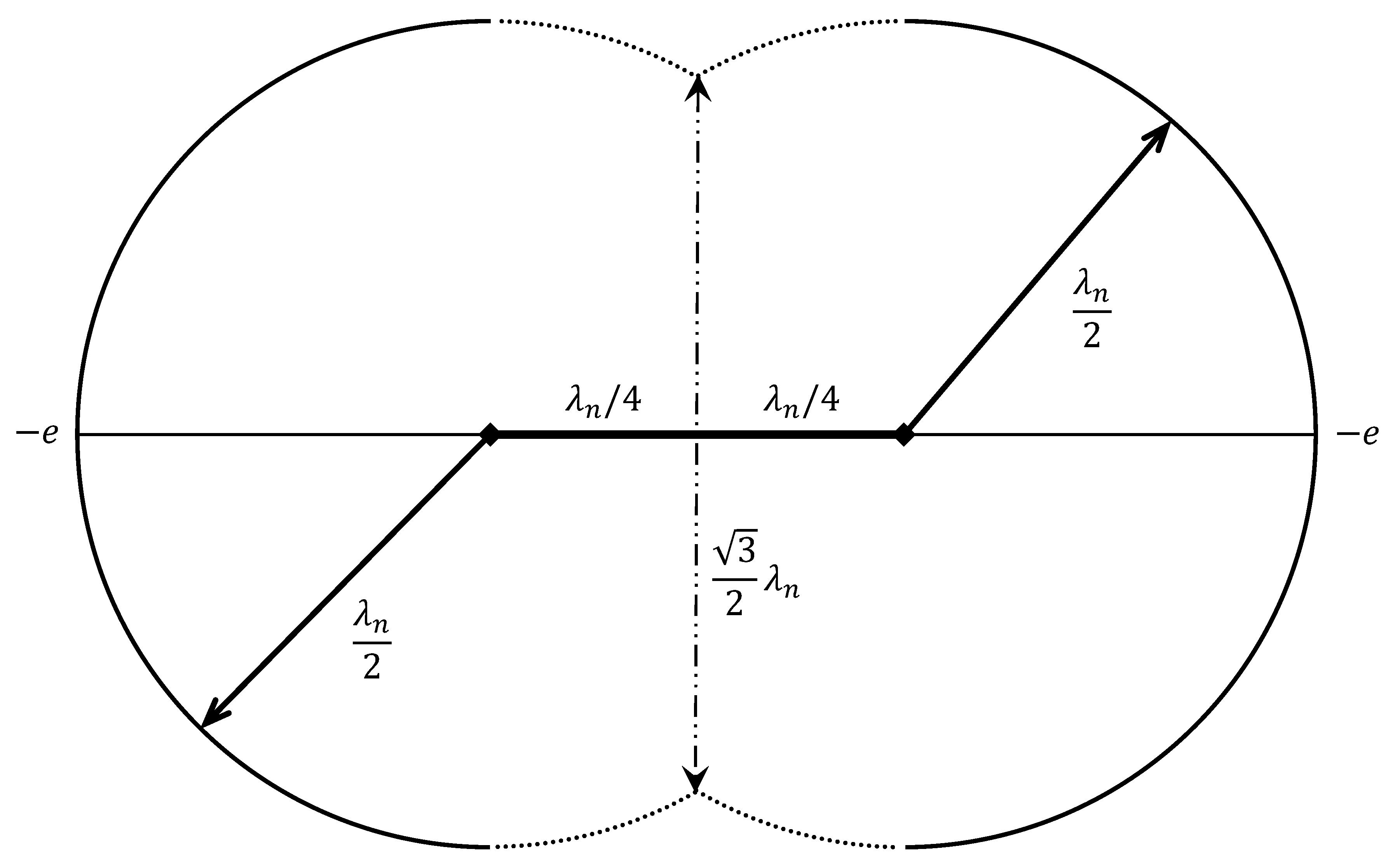
Figure 4.
Inner charge arcs of the unbound GSQV neutron, where is neutron Compton wavelength. Each charge arc is of radius , extends for radians, and is charged . A poloidally and toroidally rotating virtual vacuum fundamental harmonic connects each arc to its radial center. The two radial centers are connected by a virtual standing vacuum wave that revolves toroidally at light speed. The horizontal line represents the equatorial diameter formed by the outer charge arcs in Figure 3. The inner and outer vectors cannot overlap. The two polar points, separated by , are connected by virtual standing vacuum waves.
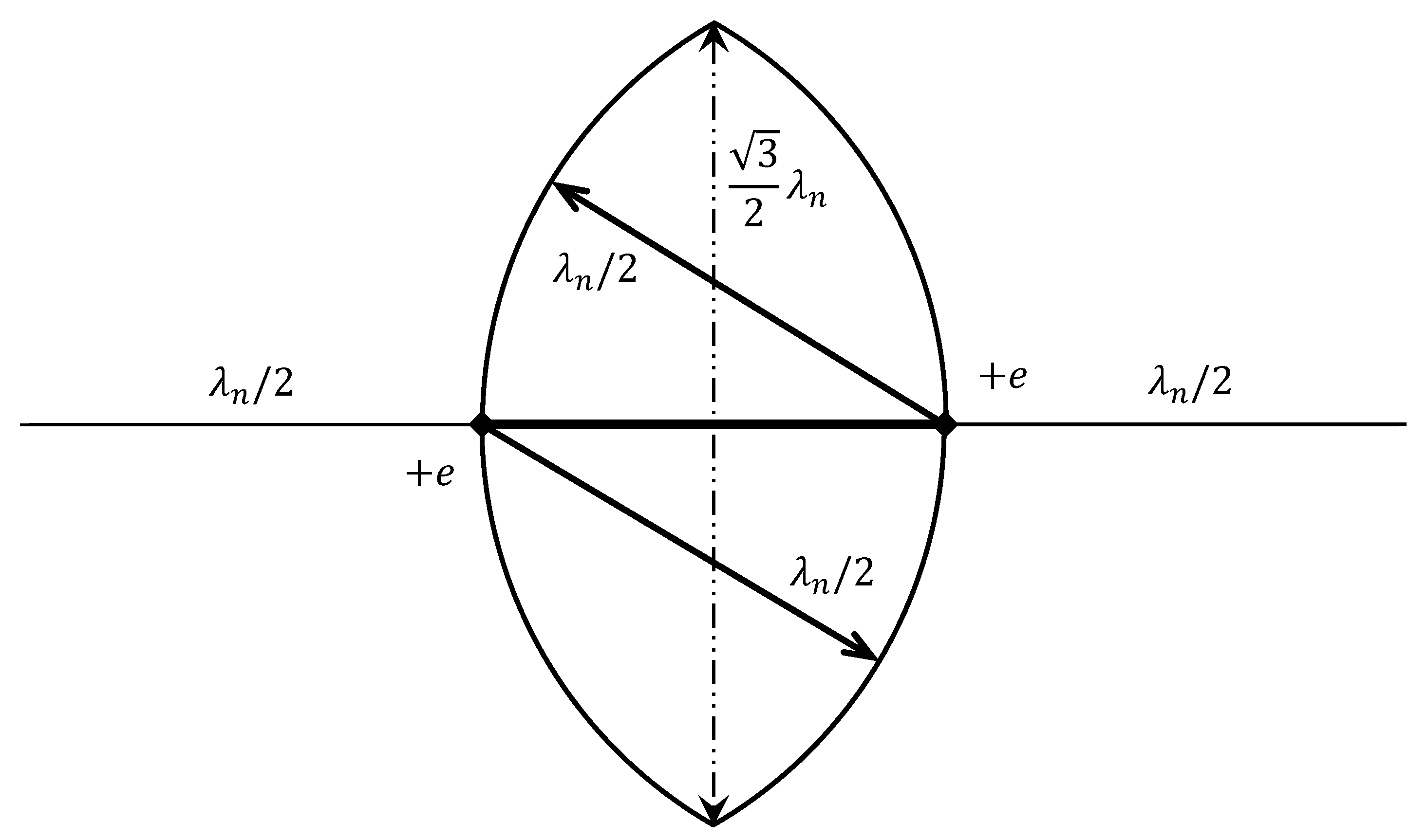
Figure 5.
Coupled charge and mass regeneration may be described in terms of virtual Möbius bands. To form a Möbius band, the sides of length are joined following a half turn.
Figure 5.
Coupled charge and mass regeneration may be described in terms of virtual Möbius bands. To form a Möbius band, the sides of length are joined following a half turn.

Figure 6.
In the unbound GSQV proton’s polar regions, virtual poloidal flow splits into two paths of equal magnitude. Dotted paths are uncharged. The revolving outer charge arcs are connected via a line that forms an uncharged virtual flat cap.
Figure 6.
In the unbound GSQV proton’s polar regions, virtual poloidal flow splits into two paths of equal magnitude. Dotted paths are uncharged. The revolving outer charge arcs are connected via a line that forms an uncharged virtual flat cap.
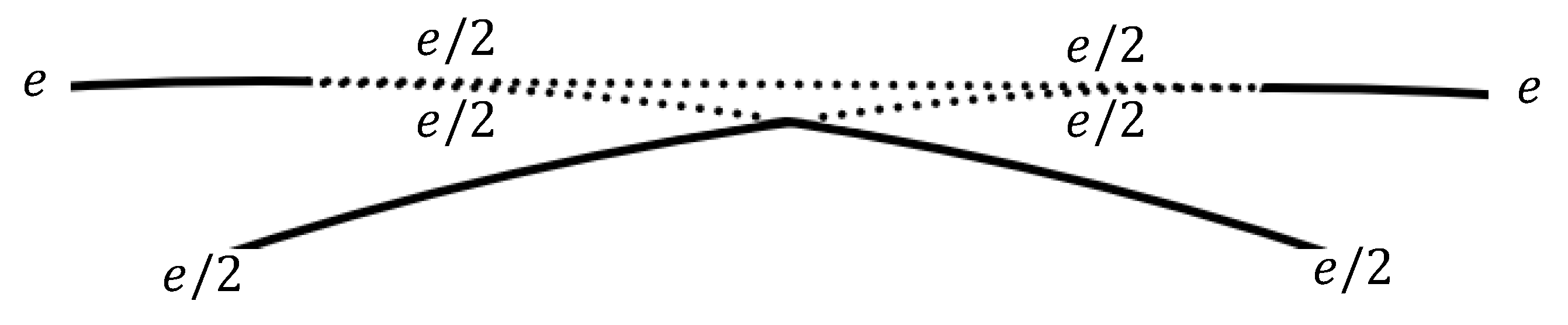
Figure 7.
Minimally excited unbound GSQV nucleons. Each circle represents a quark. Dashed outlines represent anticolors. Gluons are continually exchanging color charge. (a), The three quarks in the left-hand column transition from the two inner charge arcs of the GSQV neutron. These momentarily form a color-neutral quark triplet. The four quarks in the right-hand column transition from the two outer charge arcs of the GSQV neutron. These momentarily form a color-neutral quark quartet. The three quarks between the dashed lines connect via gluon flux tubes to form the neutron’s color-neutral valence quark triplet. (b), The two quarks in the left-hand column transition from the two inner charge arcs of the GSQV proton. These momentarily form a color-neutral quark doublet. The three quarks in the right-hand column transition from the two outer charge arcs of the GSQV proton. These momentarily form a color-neutral quark triplet. The three quarks below the dashed line connect via gluon flux tubes to form the proton’s color-neutral valence quark triplet.
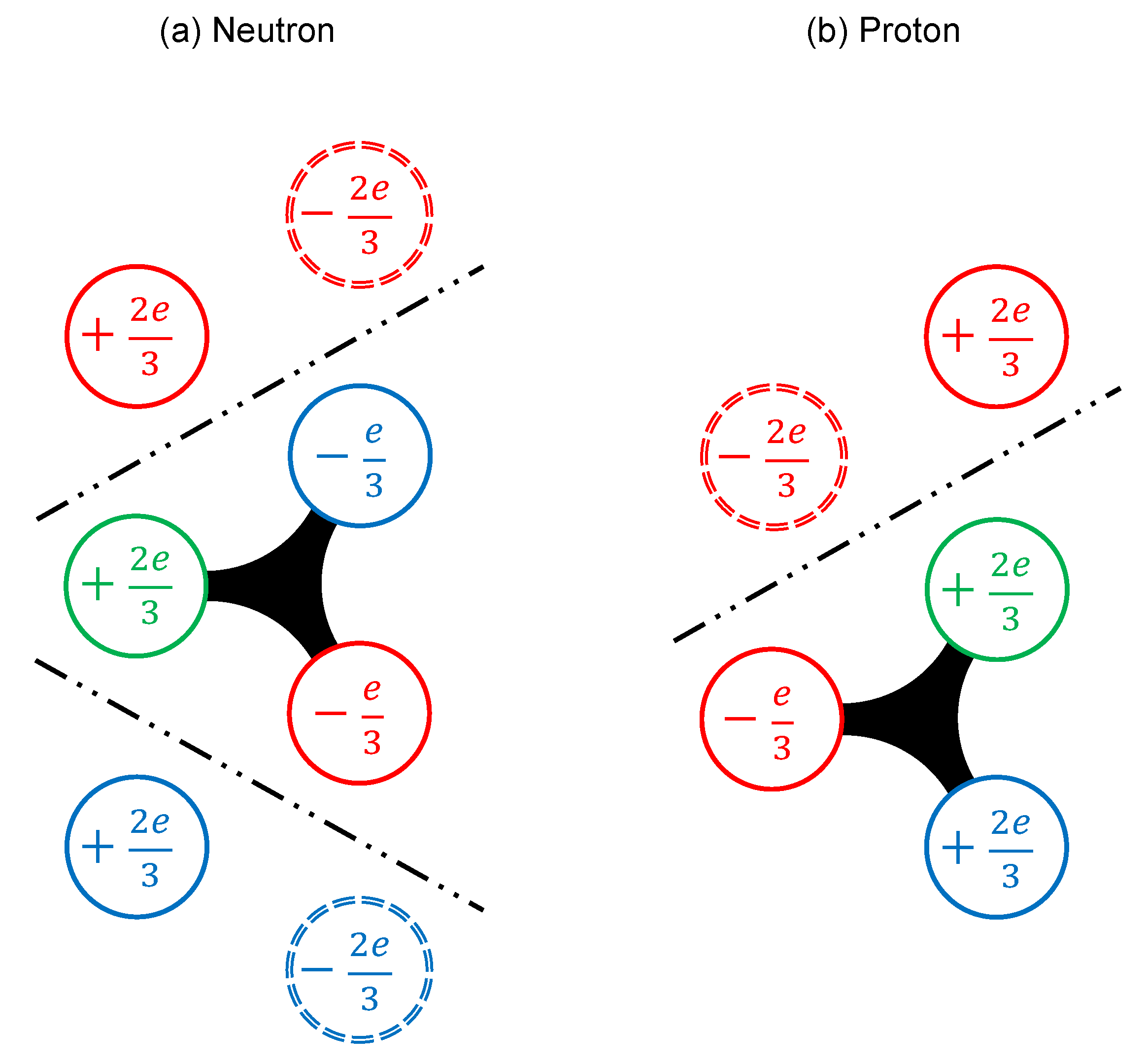
Disclaimer/Publisher’s Note: The statements, opinions and data contained in all publications are solely those of the individual author(s) and contributor(s) and not of MDPI and/or the editor(s). MDPI and/or the editor(s) disclaim responsibility for any injury to people or property resulting from any ideas, methods, instructions or products referred to in the content. |
© 2025 by the authors. Licensee MDPI, Basel, Switzerland. This article is an open access article distributed under the terms and conditions of the Creative Commons Attribution (CC BY) license (http://creativecommons.org/licenses/by/4.0/).
Copyright: This open access article is published under a Creative Commons CC BY 4.0 license, which permit the free download, distribution, and reuse, provided that the author and preprint are cited in any reuse.


