
Submitted:
02 January 2024
Posted:
04 January 2024
You are already at the latest version
Abstract
Topological states of matter have attracted significant attention due to their intrinsic wave-guiding and localization capabilities robust against disorders and defects in electronic, photonic, and phononic systems. Despite the above topological features phononic crystals share with their electronic and photonic counterparts, finite-frequency topological states in phononic crystals may not always survive. In this work, we discuss the survivability of topological states in Su-Schrieffer-Heeger models with both local and non-local interactions with larger symmetry perturbation. Although such a discussion is still about ideal mass-spring models, the insights from this study set the expectations in continuum phononic crystals, which can further instruct the applications of phononic crystals for practical purposes.
Keywords:
Topological States
; Phononic Crystals
; Chiral Symmetry
; Phonon Bandgap
1. Introduction
Topological insulators (TIs) are intrinsically electrical insulators with conducting surfaces/edges/corners when interfaced with trivial insulators, including vacuum. These surface/edge/corner states result from TI bulk properties, i.e., topological invariants, thus robust against local perturbations and disorders [1], making them ideal candidates for various promising applications in electronics strict in dissipation, especially in quantum-computing systems [2], and have thus attracted significant attention. Moreover, in recent years, these topologically protected non-dissipative localized states have inspired studies of classical analogs of TIs in photonic [3,4,5,6,7], magnetic [8,9,10], and mechanical [11,12,13,14,15,16,17] systems.
In mechanical systems, a similar topological invariant can also be derived from the spectral evolution of eigenvectors of the dynamical matrix (or the compatibility matrix) from a unit cell analysis. The integer topological invariant can then inform of the numbers and types of topologically protected surface/edge/corner states confining static deformation [18,19,20,21,22] or vibration [11,13,14,15,16,17,23,24,25] within a bulk bandgap (which is a frequency range with no eigenfrequency solutions, , bulk wave propagation) when a material/structure with a non-zero topological invariant, i.e., a topologically non-trivial phase, forms a domain wall with another domain characterized by a zero-topological invariant, i.e., a topologically trivial phase, including vacuum. Such a bulk property reflected as surface/edge/corner states at a domain wall or edge is usually referred to as the bulk-edge correspondence.
A commonly used example to illustrate this bulk-edge correspondence is the one-dimensional (1D) Su-Schrieffer-Heeger (SSH) lattice, as shown in Figure 1(a). With alternating spring constants connecting identical masses, m, a bulk bandgap can be opened as shown in Figure 1(b). It has been well established that the larger the difference in these spring constants is, the wider the bandgap we can obtain. In the existing literature, the finite-frequency in-gap topological modes are commonly created by seaming two domains with a difference in topology, here, we refer to as the topologically protected domain-wall states (TPDWSs) [15,17,26], or by simply placing a lattice with a free or fixed edge, usually cited as the “topologically protected edge states" (TPESs) [27,28,29,30,31]. However, as discussed in Refs. [28,29], the existence of these edge states and their frequencies (in case they exist) depend heavily on the boundary conditions in finite lattices, making these edge states less robust. This is because such boundaries perturb the chiral symmetry of the system’s dynamical matrix. Strictly speaking, these edge states are no longer topologically protected due to the loss of chiral symmetry. In fact, this is also the case if a domain boundary is formed between two domains with different topologies when a large perturbation to the unit cell symmetry is introduced, which, however, has received much less attention since most discussions on TPDWSs introduce a small perturbation in spring stiffness to open the bandgap in order to preserve the chiral symmetry to some extent. Nonetheless, a large bandgap is usually desirable in many applications requiring vibration mitigation within a certain frequency range [32,33,34,35]. Hence, it is important to identify the conditions for the survivability of the in-gap states. Since these in-gap states are deviations from TPESs or TPDWSs, some topological features at these boundaries still exist even with large chiral symmetry perturbation.
In this work, we will delve into SSH systems with large symmetry perturbations at the domain boundary and the unit cell. Simple SSH chains with nearest-neighbor interactions only and the more complex SSH networks with beyond-nearest-neighbors (BNNs) will both be taken into account, the latter of which is gaining rising attention lately due to their roton-like dispersion relations similar to those in correlated quantum systems [36,37,38,39,40,41], as well as their unconventional topological states associated with the BNN coupling [17,42,43,44]. The survivability of the in-gap states will be analyzed, which will further instruct the design of large-bandgap structures in the continuum regime.
2. Results and Discussion
2.1. Su-Schrieffer-Heeger Systems with Nearest-Neighbor Interactions
To simplify the illustration, we only consider displacements of identical masses, m, connected by alternating nearest-neighbor springs with spring constants and along the chain, as shown in Figure 1(a). The governing equations of a lattice unit cell can be expressed as
where displacements of the two masses in the p-th cell are denoted as and , respectively. The displacements of masses in any unit cell p at time t can be expressed by the ones within a reference unit cell using a plane-wave solution in combination with Bloch-Floquet periodic boundary conditions:
where is the vibration frequency, are the displacements of the p-th cell with , q is the wave number, which is inversely proportional to the wavelength , i.e., , a denotes the lattice constant, are displacements within the reference unit cell. Substituting this expression in Eqns. 1 and gives:
where is the stiffness (or dynamical) matrix of the periodic system:
The square root of the eigenvalues of gives the phonon band diagram, as presented in Figure 1(b). With , there is no bandgap between the two bands. When , a bandgap is created between the two phonon bands due to the breaking of the unit cell space-inversion-symmetry (SIS). Although the bandgap does not alter if or vice versa, The two choices of gauge result in two different topological states since the transition from one to another unavoidably passes the non-gap state, , non-gapped transition, as shown in the middle panels of Figure 1(b–d). To characterize the topology of such a 1D system, the Zak phase [45] measuring the rotation of eigenvectors in the unit cell, or the winding number n are often evaluated, as shown in Figure 1(d). The latter of which is defined as
where is the unitary matrix, is the chiral matrix after subtracting all diagonal elements:
where is the identity matrix. The eigenvalues of present to be symmetric about the x-axis, as shown in Figure 1(c).
As we can see, when , , indicating a trivial intra-cell-hopping phase. On the contrary, when , , suggesting a topologically nontrivial inter-cell-hopping phase. Such a difference in topology due to gauge choice suggests that if connecting two domains with these two different topologies, there exists a localized mode with a frequency located within the bandgap at the domain wall.
In this section, we will discuss the effect of the boundary conditions on the existence of in-gap states when a simple mass-spring lattice shown in Figure 1(a) is interfaced with a vacuum (Subsection In-Gap Edge States in Finite Lattices) and with a domain with an opposite gauge in the unit cell (Subsection In-Gap Domain-Wall States in Infinite Lattices) with various characterizing the difference between and , defined as and . Here, we consider a wide range of , up to , which is of the average spring stiffness (we set ). Such a big difference in the spring constants will create a large bulk bandgap, which, as mentioned in the Introduction, is desirable for many applications. However, the survivability of the in-gap states depends on the specific boundary condition.
2.1.1. In-Gap Edge States in Finite Lattices
To start with, we take a finite lattice containing 20 unit cells presented in Figure 1(a) with free boundaries, as shown in Figure 2(a). The stiffness matrix of such a finite system is:
As we can see, is not a chiral matrix due to non-identical diagonal elements at the two free boundaries. Hence, no in-gap states exist, as shown in Figure 2(a–d), regardless of .
The in-gap edge states can be easily acquired by fixing the two ending masses with a spring, , connected to a wall, as shown in Figure 2(e), making the chiral:
Subtracting the diagonal elements as in Eqn. 7 also gives us a chiral matrix . In this case, as long as the SSH terminating cells present a nontrivial gauge, , or , and are interfaced with vacuum – a trivial domain, the in-gap edge states guarantee to exist regardless of the magnitude of , as evident in Figure 2(f–h). Moreover, due to the strict chiral symmetry Eqn. 9 presents, all the in-gap edge states are located exactly at in the eigenfrequency plot in Figure 2(f), or in the eigenvalue plot in Figure 2(g), which we refer to as the mid-gap state in our discussion. These in-gap edge states completely follow the definition of TPESs, also known as the Jackiw-Rebbi zero modes [46].
However, despite being topologically protected, these TPESs are prone to boundary conditions. A small perturbation at the edges will drift the TPESs away from the mid-gap state, or make them disappear, as shown in Figure 2(i,j). Thus, topology alone can no longer guarantee the existence of TPESs. A chiral symmetry of the entire system is crucial to achieve TPESs. On the other hand, even when the chain terminates with topologically trivial unit cells on both ends, one in-gap state on both ends may still emerge with a sufficiently large , as presented in Figure 2(k). This in-gap state, nonetheless, is merely a trivial edge state due to the termination of periodicity.
2.1.2. In-Gap Domain-Wall States in Infinite Lattices
When seaming two topologically different domains, as shown in Figure 3(a), to obtain TPDWSs, a chiral symmetry of the dynamical matrix, , of the entire system must also be maintained. Without any modification, of a supercell shown in Figure 3(a), in which the Bloch-Floquet boundary conditions are applied to the top and bottom masses, writes:
which is not a chiral matrix due to the domain-wall mass connected to on both sides. Although we can achieve a chiral matrix by pinning the domain-wall mass, it is not realistic in practice and highly challenging when .
When the difference between and , or , is small, does not significantly deviate from a chiral matrix, thus the in-gap state is still adjacent to the middle of the bandgap, as shown in Figure 3(b,c). However, when and are largely different, can no longer be approximated as a chiral matrix. Interestingly, when , , , the in-gap state is intact. The breaking of the chiral symmetry of results in an additional trivial edge mode arising above the upper limit of the bulk mode. On the contrary, when , the in-gap state drops quickly near the lower bulk mode as increases. Although unlike in finite lattices, such an in-gap state always survives, it is not easy to detect due to its proximity to the bulk mode. Mode shapes when are presented in Figure 3(d). The mid-gap state when decays rapidly due to a large bandgap. In contrast, when , the domain-wall state decays slowly into the bulk since its frequency is merely slightly above the bulk mode.
2.2. Su-Schrieffer-Heeger Systems with Beyond-Nearest-Neighbor Interactions
Introducing non-local or BNN interactions further complicates the discussion. In this section, we will discuss systems with identical third-nearest neighbors (TNNs) but the nearest neighbors are non-identical, , and , and vice versa, as shown in Figure 4.
The additional TNNs connect the current cell, p, with the one beyond its immediate neighbors, , , modifying the governing equations to be:
Plugging in Eqn. (3), we get the stiffness matrix as:
The chiral matrix can then be obtained from,
The additional exponential terms in Eqns. 11 and , or in the off-diagonal terms in (Eqn. 13) due to TNNs yield the bending of the dispersion curves in the irreducible Brillouin zone (IBZ), as shown in Figure 4(b,c), also known as the roton-like acoustic dispersion, similar to those discovered at cryogenic temperatures in correlated quantum systems [36,37,38,39,40,41].
Although phonon dispersions due to different nearest neighbors and TNNs are almost identical, their winding paths differ significantly. When and , with two extra local loops formed along the path, while when and , since the circuit winds about the origin in the opposite direction (clockwise) to that of the main path. Such a difference in winding number indicates that the former lattice is topologically trivial, while the latter one is nontrivial. On the contrary, when and , with three local loops formed along the path, while when and , the circuit winds about the origin twice counterclockwise, thus , indicating both being non-trivial. This suggests that when interfacing the lattice of with a vacuum or a topologically trivial domain, n edge/domain-wall states should exist. However, previously, we have demonstrated that this is not necessarily correct. We mathematically demonstrated that the number of domain-wall states when seaming two topologically different domains is determined by the number of band crossings when and within the IBZ, or Dirac points, which is the phonon realization of the Jackiw-Rebbi theory [46]. We found that the actual number of TPDWSs can be characterized by the Berry connection calculated from the integrant of Eqn. 6, or local winding numbers, instead of the total winding numbers over the IBZ [17]. Nonetheless, the total winding numbers across the whole IBZ as shown in Figure 4(d) may still inform the number of edge states when a lattice is terminated and interfaced with a vacuum.
In this section, we will discuss the effect of a combination of the spring difference (both and , the latter of which is defined as and ) and boundary conditions on the existence of in-gap states when a mass-spring lattice with TNNs shown in Figure 4(a) is interfaced with a vacuum (Subsection In-Gap Edge States in Finite Lattices with Third-Nearest Neighbors) and with a topologically different domain (Subsection In-Gap Domain-Wall States in Infinite Lattices with Third-Nearest Neighbors). We consider the scenarios across both a wide range of and , up to 0.9, which opens a large bandgap. The conditions of maintaining the in-gap states will be explored.
2.2.1. In-Gap Edge States in Finite Lattices with Third-Nearest Neighbors
Taking a finite lattice containing 20 unit cells with free boundaries, as shown in Figure 5(a), yields the stiffness matrix as:
Again, is not a chiral matrix due to non-identical diagonal elements close to the two free boundaries. Therefore, we expect there not to be any in-gap states. However, this is not the case when and , as shown in Figure 5(b–d). On the other hand, when and , there are no in-gap states, Figure 6(a–d), consistent with the observation when masses are only connected by nearest neighbors, as in Figure 2(a–d). In the former scenario, although these in-gap states are indeed edge states, the two in-gap mode numbers are 22 and 23 when , and 21 and 22 when . In the case of topological in-gap states, the mode numbers should be 20 and 21 for a finite chain containing 20 unit cells. In addition, there is a significant leakage of the edge modes into the bulk compared to those shown in Figure 5(h) when the edges are fixed so that and (as defined in Eqn. 14) are chiral:
as shown in Figure 5(e). Hence, the two in-gap edge states in the lattice with free boundaries shown in Figure 5(a–d) are trivial edge modes, whose existence is independent of its topology.
On the other hand, when fixing the masses near the two edges with appropriate springs to the ground/wall to make chiral as in Eqn. 16, the number of TPESs appear exactly as predicted by their corresponding winding numbers. When and , there are no in-gap states since . While when and , one in-gap state exists at each edge, matching , as shown in Figure 5(f,g). Similarly, when and , , corresponding to the two mid-gap states when , Figure 5(g). The opposite arrangement of TNNs, , yields two edge states at each end, as shown in Figure 5(h), matching its topological invariant, .
2.2.2. In-Gap Domain-Wall States in Infinite Lattices with Third-Nearest Neighbors
By seaming two domains of lattices with different winding numbers, we can, again, form a domain wall, as shown in Figure 7(a). Nonetheless, with the incorporation of TNNs, the domain wall is not a single mass as shown in Figure 3(a). Here, the interfacial mass connected by on both sides serves as the domain-wall mass for the nearest neighbors. This domain-wall mass is also connected by on both sides. One additional mass on each side of this domain-wall mass is connected by on both sides. Hence, these three masses, altogether, serve as the domain-wall mass for the TNNs. then writes:
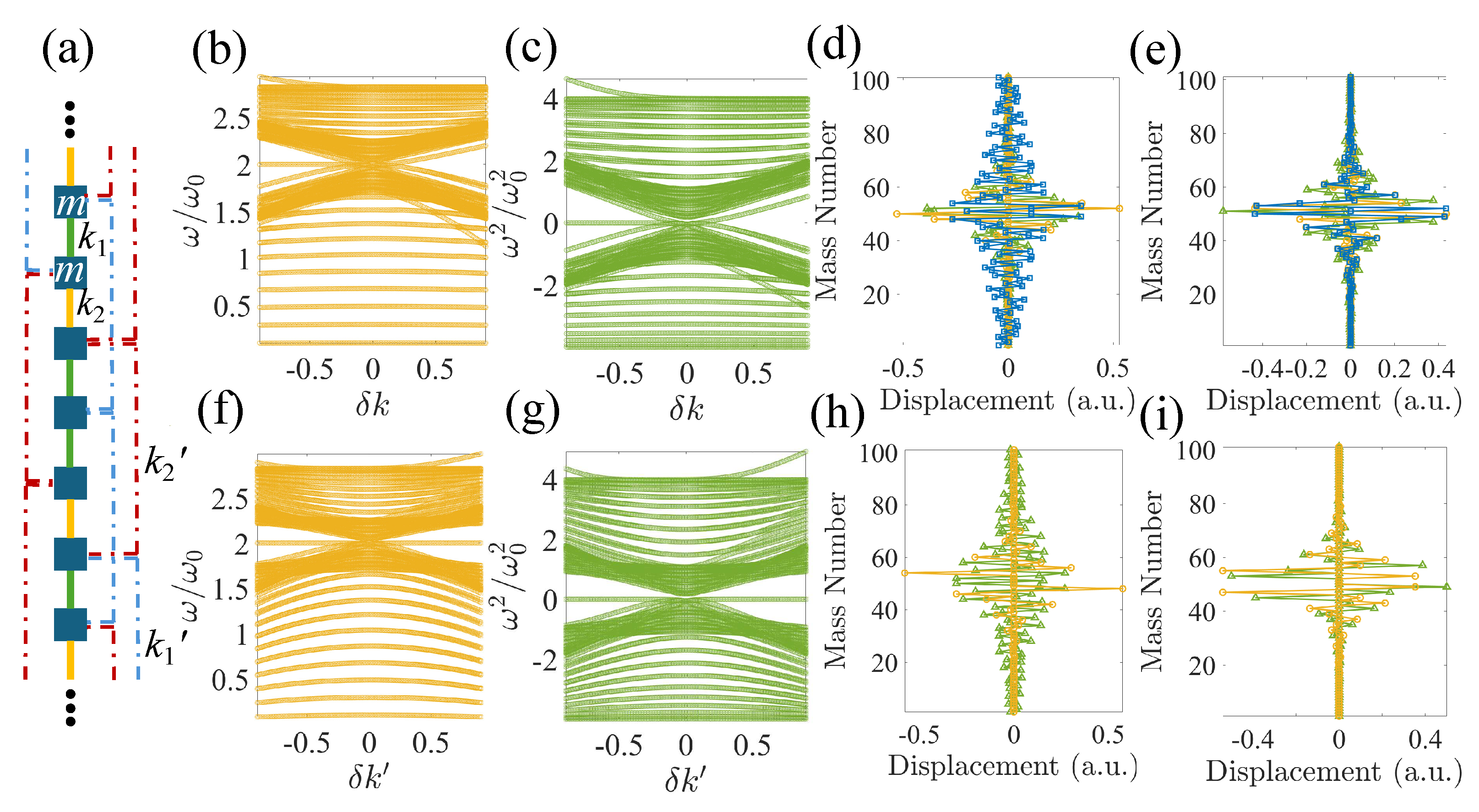
As we can see, the spring arrangements at the three domain-wall masses prevent from being chiral. Unless connecting them with extra springs to a fixed wall to remove the three non-zero diagonal elements in Eqn. 17, which is not practical, especially when or , we expect to observe strong deviation of the in-gap states from mid-gap.
In the case of , we have previously demonstrated that the winding numbers shown in Figure 4(d) can no longer correctly predict the number of TPDWSs. Instead, local winding numbers derived from the Berry connection inform us of three TPDWSs if is set to be chiral [17]. Without any modification around the domain wall, as increases, although the three in-gap states still exist, as shown in Figure 7(b) and (c), when , only one in-gap state remains at the mid-gap, two of them get extremely close to the bulk modes, resulting in significant leakage of the domain-wall states into the bulk, as shown in Figure 7(d). When , all three in-gap states survive in the bandgap, but with a large deviation from the mid-gap. Thus, the domain-wall states still leak into the bulk, as shown in fig. Figure 7(e), compared to those with small .
As we vary while keeping , both the winding number and Berry connection calculation predict that there should be three in-gap states at the domain wall. However, from Figure 7(f,g), this is only the case when . As increases, when , only one mode remains mid-gap, one other gets extremely close to the lower bulk band, resulting in slow spatial decay from the domain boundary, and the third one completely disappears, as shown in Figure 7(h). While when , the two surviving in-gap states are located at the mid-gap state, thus, with rapid spatial decay, Figure 7(i), and the third in-gap mode no longer exists within the bulk bandgap. It, instead, migrates to above the top bulk band.
3. Conclusion
In this work, we use Su-Schrieffer-Heeger models to thoroughly compare the effect of various boundary conditions on the survivability of in-gap states within bulk bandgaps and their relationship with topologically protected edge/domain-wall states. We find that the in-gap edge states never exist when lattice boundaries are free since the stiffness matrix largely deviates from being chiral. The occasional observed localized edge modes only occur by accident due to specific spring arrangements. They are not topologically protected and leak much into the bulk. On the other hand, fixing the free ends to the ground with proper spring constants to ensure the chirality of the stiffness matrix guarantees the topologically protected edge states when the lattice arrangement is topological. The edge states are also strongly localized on the edges. On the other hand, the in-gap domain-wall states formed by two topologically different domains are much more tolerant to the non-chirality of the stiffness matrix, although not all in-gap states will survive with a large difference in the third-nearest neighbors. Interestingly, when the domain-wall mass is connected by stiffer springs, the mid-gap states are always retained and preserve most of the topological features, such as rapid spatial decay, which is not the case when the domain-wall mass is connected by softer springs.
Although we use discrete mass-spring models in our study, the conclusions are expandable to the continuum regime and can be used to distinguish and explain the difference between topological and trivial edge/domain-wall states in continuous structures in practical applications.
Author Contributions
Both authors have contributed equality to the manuscript and have read and agreed to the published version of the manuscript.
Funding
This research received no external funding.
Data Availability Statement
The datasets generated during and/or analyzed during the current study are available from the corresponding author upon reasonable request.
Conflicts of Interest
The authors declare no conflict of interest.
Abbreviations
The following abbreviations are used in this manuscript:
| TI | Topological insulator |
| 1D | One dimension(al) |
| SSH | Su-Schrieffer-Heeger |
| TPES | Topologically protected edge state |
| TPDWS | Topologically protected domain-wall state |
| BNN | Beyond-nearest neighbor |
| TNN | Third-nearest neighbor |
| SIS | Space inversion symmetry |
| IBZ | Irreducible Brillouin zone |
References
- Hasan, M.Z.; Kane, C.L. Colloquium: topological insulators. Reviews of modern physics 2010, 82, 3045. [Google Scholar] [CrossRef]
- He, M.; Sun, H.; He, Q.L. Topological insulator: Spintronics and quantum computations. Frontiers of Physics 2019, 14, 1–16. [Google Scholar] [CrossRef]
- Lu, L.; Joannopoulos, J.D.; Soljačić, M. Topological photonics. Nature photonics 2014, 8, 821–829. [Google Scholar] [CrossRef]
- Yang, Y.; Xu, Y.F.; Xu, T.; Wang, H.X.; Jiang, J.H.; Hu, X.; Hang, Z.H. Visualization of a unidirectional electromagnetic waveguide using topological photonic crystals made of dielectric materials. Physical review letters 2018, 120, 217401. [Google Scholar] [CrossRef] [PubMed]
- Wang, H.; Gupta, S.K.; Xie, B.; Lu, M. Topological photonic crystals: a review. Frontiers of Optoelectronics 2020, 13, 50–72. [Google Scholar] [CrossRef] [PubMed]
- Tang, G.J.; He, X.T.; Shi, F.L.; Liu, J.W.; Chen, X.D.; Dong, J.W. Topological photonic crystals: physics, designs, and applications. Laser & Photonics Reviews 2022, 16, 2100300. [Google Scholar]
- Hafezi, M.; Mittal, S.; Fan, J.; Migdall, A.; Taylor, J. Imaging topological edge states in silicon photonics. Nature Photonics 2013, 7, 1001–1005. [Google Scholar] [CrossRef]
- Zhang, R.X.; Liu, C.X. Topological magnetic crystalline insulators and corepresentation theory. Physical Review B 2015, 91, 115317. [Google Scholar] [CrossRef]
- Tokura, Y.; Yasuda, K.; Tsukazaki, A. Magnetic topological insulators. Nature Reviews Physics 2019, 1, 126–143. [Google Scholar] [CrossRef]
- Malki, M.; Uhrig, G. Topological magnetic excitations. Europhysics Letters 2020, 132, 20003. [Google Scholar] [CrossRef]
- Wang, P.; Lu, L.; Bertoldi, K. Topological phononic crystals with one-way elastic edge waves. Physical review letters 2015, 115, 104302. [Google Scholar] [CrossRef]
- Tian, Z.; Shen, C.; Li, J.; Reit, E.; Bachman, H.; Socolar, J.E.; Cummer, S.A.; Jun Huang, T. Dispersion tuning and route reconfiguration of acoustic waves in valley topological phononic crystals. Nature communications 2020, 11, 762. [Google Scholar] [CrossRef] [PubMed]
- Ma, J. Phonon Engineering of Micro-and Nanophononic Crystals and Acoustic Metamaterials: A Review. Small Science 2023, 3, 2200052. [Google Scholar] [CrossRef]
- Ma, J.; Zhou, D.; Sun, K.; Mao, X.; Gonella, S. Edge modes and asymmetric wave transport in topological lattices: Experimental characterization at finite frequencies. Physical review letters 2018, 121, 094301. [Google Scholar] [CrossRef] [PubMed]
- Ma, J.; Sun, K.; Gonella, S. Valley hall in-plane edge states as building blocks for elastodynamic logic circuits. Physical Review Applied 2019, 12, 044015. [Google Scholar] [CrossRef]
- Zhou, D.; Ma, J.; Sun, K.; Gonella, S.; Mao, X. Switchable phonon diodes using nonlinear topological Maxwell lattices. Physical Review B 2020, 101, 104106. [Google Scholar] [CrossRef]
- Rajabpoor Alisepahi, A.; Sarkar, S.; Sun, K.; Ma, J. Breakdown of conventional winding number calculation in one-dimensional lattices with interactions beyond nearest neighbors. Communications Physics 2023, 6, 334. [Google Scholar] [CrossRef]
- Kane, C.L.; Lubensky, T.C. Topological boundary modes in isostatic lattices. Nature Physics 2014, 10, 39–45. [Google Scholar] [CrossRef]
- Paulose, J.; Chen, B.G.g.; Vitelli, V. Topological modes bound to dislocations in mechanical metamaterials. Nature Physics 2015, 11, 153–156. [Google Scholar] [CrossRef]
- Rocklin, D.Z.; Zhou, S.; Sun, K.; Mao, X. Transformable topological mechanical metamaterials. Nature communications 2017, 8, 14201. [Google Scholar] [CrossRef] [PubMed]
- Rocklin, D.Z.; Chen, B.G.g.; Falk, M.; Vitelli, V.; Lubensky, T. Mechanical Weyl modes in topological Maxwell lattices. Physical review letters 2016, 116, 135503. [Google Scholar] [CrossRef] [PubMed]
- Bilal, O.R.; Süsstrunk, R.; Daraio, C.; Huber, S.D. Intrinsically polar elastic metamaterials. Advanced Materials 2017, 29, 1700540. [Google Scholar] [CrossRef] [PubMed]
- Süsstrunk, R.; Huber, S.D. Observation of phononic helical edge states in a mechanical topological insulator. Science 2015, 349, 47–50. [Google Scholar] [CrossRef] [PubMed]
- Nash, L.M.; Kleckner, D.; Read, A.; Vitelli, V.; Turner, A.M.; Irvine, W.T. Topological mechanics of gyroscopic metamaterials. Proceedings of the National Academy of Sciences 2015, 112, 14495–14500. [Google Scholar] [CrossRef]
- Mousavi, S.H.; Khanikaev, A.B.; Wang, Z. Topologically protected elastic waves in phononic metamaterials. Nature communications 2015, 6, 8682. [Google Scholar] [CrossRef] [PubMed]
- Pal, R.K.; Ruzzene, M. Edge waves in plates with resonators: an elastic analogue of the quantum valley Hall effect. New Journal of Physics 2017, 19, 025001. [Google Scholar] [CrossRef]
- Allein, F.; Anastasiadis, A.; Chaunsali, R.; Frankel, I.; Boechler, N.; Diakonos, F.K.; Theocharis, G. Strain topological metamaterials and revealing hidden topology in higher-order coordinates. Nature Communications 2023, 14, 6633. [Google Scholar] [CrossRef] [PubMed]
- Rosa, M.I.; Davis, B.L.; Liu, L.; Ruzzene, M.; Hussein, M.I. Material vs. structure: Topological origins of band-gap truncation resonances in periodic structures. Physical Review Materials 2023, 7, 124201. [Google Scholar] [CrossRef]
- Kuo, J.Y.; Lee, T.Y.; Chiu, Y.C.; Liao, S.R.; Kao, H.c. SSH coupled-spring systems. arXiv preprint arXiv:2310.00547, arXiv:2310.00547 2023.
- Coutant, A.; Sivadon, A.; Zheng, L.; Achilleos, V.; Richoux, O.; Theocharis, G.; Pagneux, V. Acoustic Su-Schrieffer-Heeger lattice: Direct mapping of acoustic waveguides to the Su-Schrieffer-Heeger model. Physical Review B 2021, 103, 224309. [Google Scholar] [CrossRef]
- Li, X.; Meng, Y.; Wu, X.; Yan, S.; Huang, Y.; Wang, S.; Wen, W. Su-Schrieffer-Heeger model inspired acoustic interface states and edge states. Applied Physics Letters 2018, 113. [Google Scholar] [CrossRef]
- Joubaneh, E.F.; Ma, J. Symmetry effect on the dynamic behaviors of sandwich beams with periodic face sheets. Composite Structures 2022, 289, 115406. [Google Scholar] [CrossRef]
- Yang, S.; Chang, H.; Wang, Y.; Yang, M.; Sun, T. A phononic crystal suspension for vibration isolation of acoustic loads in underwater gliders. Applied Acoustics 2024, 216, 109731. [Google Scholar] [CrossRef]
- Bendsoe, M.P.; Sigmund, O. Topology optimization: theory, methods, and applications; Springer Science & Business Media, 2003.
- Hussein, M.I.; Hamza, K.; Hulbert, G.M.; Saitou, K. Optimal synthesis of 2D phononic crystals for broadband frequency isolation. Waves in Random and Complex Media 2007, 17, 491–510. [Google Scholar] [CrossRef]
- Chen, Y.; Kadic, M.; Wegener, M. Roton-like acoustical dispersion relations in 3D metamaterials. Nature communications 2021, 12, 3278. [Google Scholar] [CrossRef] [PubMed]
- Iglesias Martínez, J.A.; Groß, M.F.; Chen, Y.; Frenzel, T.; Laude, V.; Kadic, M.; Wegener, M. Experimental observation of roton-like dispersion relations in metamaterials. Science advances 2021, 7, eabm2189. [Google Scholar] [CrossRef] [PubMed]
- Iorio, L.; De Ponti, J.M.; Maspero, F.; Ardito, R. Roton-like dispersion via polarisation change for elastic wave energy control in graded delay-lines. Journal of Sound and Vibration 2024, 572, 118167. [Google Scholar] [CrossRef]
- Cui, J.G.; Yang, T.; Niu, M.Q.; Chen, L.Q. Tunable roton-like dispersion relation with parametric excitations. Journal of Applied Mechanics 2022, 89, 111005. [Google Scholar] [CrossRef]
- Wang, K.; Chen, Y.; Kadic, M.; Wang, C.; Wegener, M. Nonlocal interaction engineering of 2D roton-like dispersion relations in acoustic and mechanical metamaterials. Communications Materials 2022, 3, 35. [Google Scholar] [CrossRef]
- Zhu, Z.; Gao, Z.; Liu, G.G.; Ge, Y.; Wang, Y.; Xi, X.; Yan, B.; Chen, F.; Shum, P.P.; Sun, H.x.; others. Observation of multiple rotons and multidirectional roton-like dispersion relations in acoustic metamaterials. New Journal of Physics 2022, 24, 123019. [Google Scholar] [CrossRef]
- Grundmann, M. Topological States Due to Third-Neighbor Coupling in Diatomic Linear Elastic Chains. physica status solidi (b) 2020, 257, 2000176. [Google Scholar] [CrossRef]
- Chen, H.; Nassar, H.; Huang, G. A study of topological effects in 1D and 2D mechanical lattices. Journal of the Mechanics and Physics of Solids 2018, 117, 22–36. [Google Scholar] [CrossRef]
- Liu, H.; Huang, X.; Yan, M.; Lu, J.; Deng, W.; Liu, Z. Acoustic Topological Metamaterials of Large Winding Number. Physical Review Applied 2023, 19, 054028. [Google Scholar] [CrossRef]
- Zak, J. Berry’s phase for energy bands in solids. Physical review letters 1989, 62, 2747. [Google Scholar] [CrossRef] [PubMed]
- Jackiw, R.; Rebbi, C. Solitons with fermion number 1/2. Physical Review D 1976, 13, 3398. [Google Scholar] [CrossRef]
Figure 1.
(a) Unit cell (circled in a dashed line) of a chain of identical masses, m, with alternating springs with spring constants (green bars) and (yellow bars). The unit cell length is a. (b)-(d): (b) Phonon dispersion curves, (c) eigenvalue plots of denoted as (both normalized by ), and (d) winding paths for (, and , left), (, , middle), and (, and , right) in the unit cell.
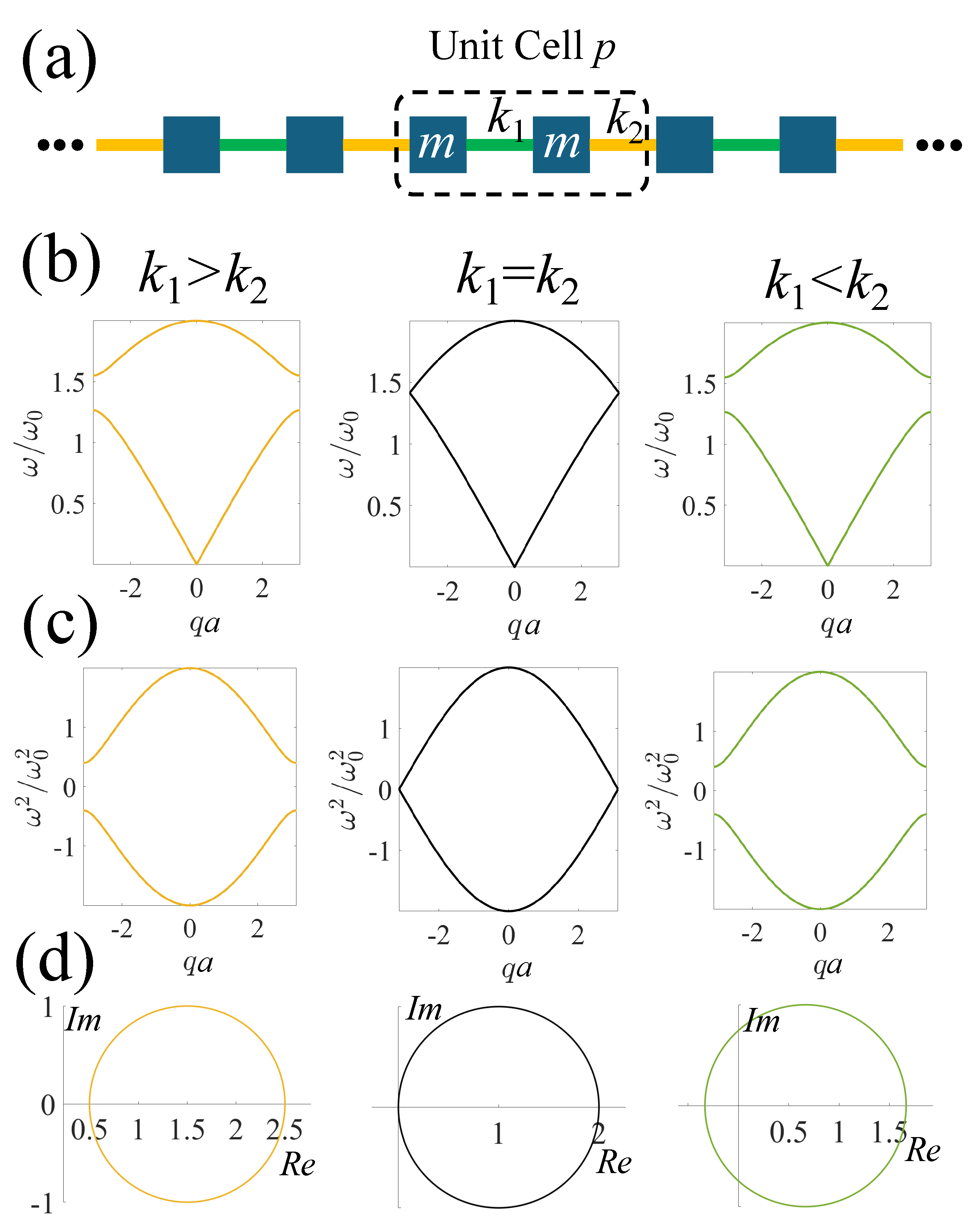
Figure 2.
(a) A finite lattice containing 20 unit cells of identical masses, m, with alternating springs with spring constants (green bars) and (yellow bars). and . (b) Normalized eigenfrequencies of the finite lattice in (a). (c) Normalized eigenvalues of the stiffness matrix of (a) after subtracting . (d) 20th (yellow circles) and 21st (green triangles) eigenmodes when . (e) Connecting the two ends of the finite lattice to a wall by springs with a constant . (f) Normalized eigenfrequencies of the finite lattice in (e). (g) Normalized eigenvalues of the stiffness matrix of (e) after subtracting . (h) 20th (yellow circles) and 21st (green triangles) eigenmodes when . (i) and (j): (i) Normalized eigenfrequencies and (j) normalized eigenvalues of the stiffness matrix after subtracting of (e) with varies and fixed and (yellow - , green - ). (k) In-gap eigen modes of (yellow circles and triangles) and (green squares) when .
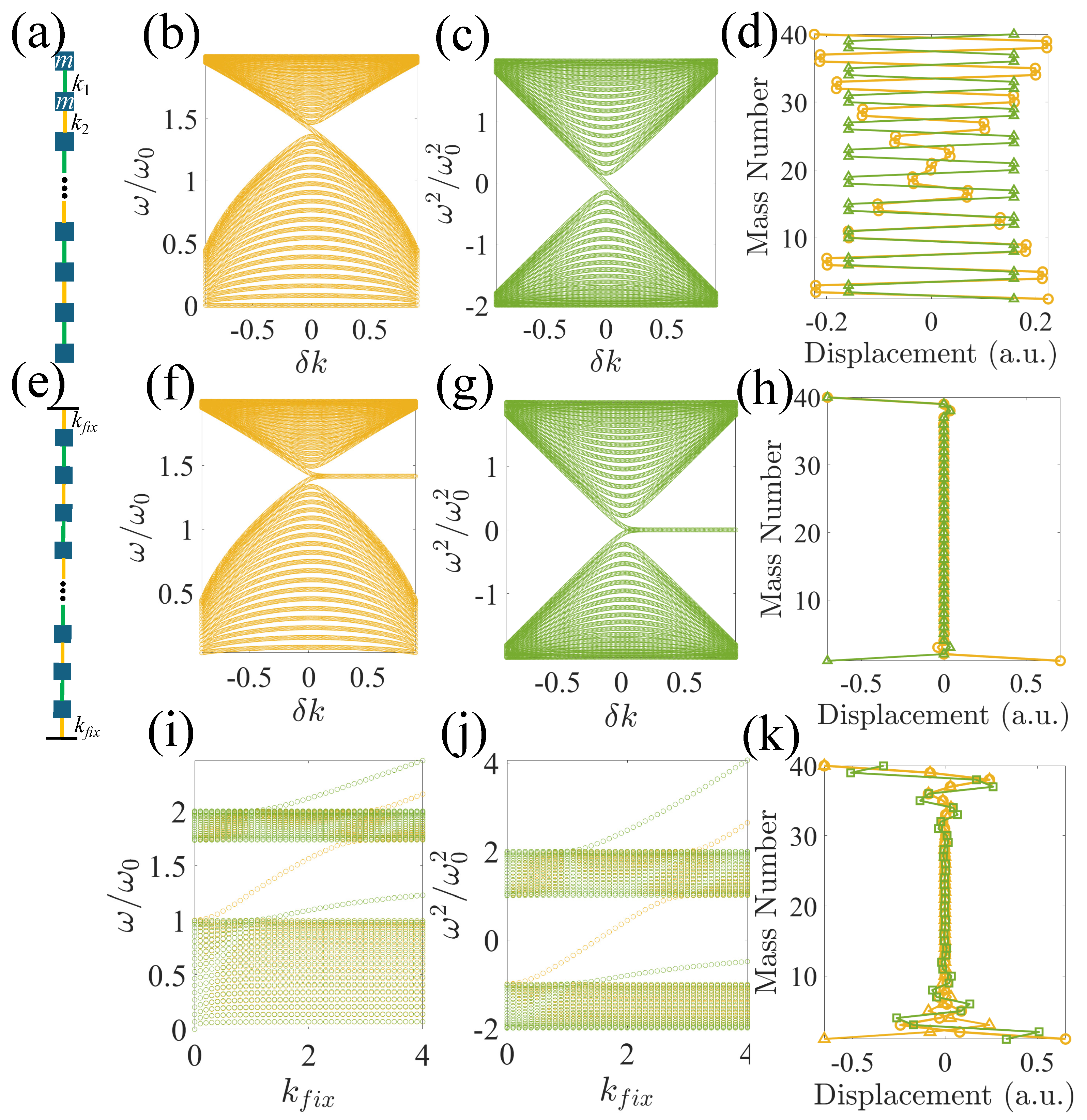
Figure 3.
(a) An infinite lattice with a supercell containing 101 identical masses, m, with alternating springs with spring constants (green bars) and (yellow bars) forming an interface at the central mass, about which connected are on both sides. and . (b) Normalized eigenfrequencies of the finite lattice in (a). (c) Normalized eigenvalues of the stiffness matrix of (a) after subtracting . (d) Supercell eigenmodes when (green triangles) and (yellow circles).
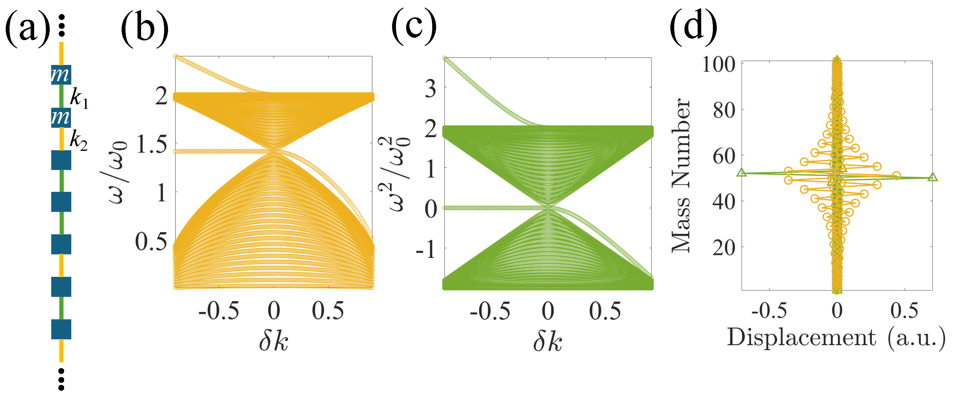
Figure 4.
(a) Unit cell (circled in a dashed line) of a chain of identical masses, m, with alternating springs, with spring constants (green bars) and (yellow bars), connecting the nearest neighbors, and (blue dashed lines) and (red dashed lines), connecting the third-nearest neighbors. The unit cell length is a. (b)-(d): (b) Phonon dispersion curves, (c) eigenvalue plots of denoted as (both normalized by ), and (d) winding paths for (, and ) and (yellow curves in the left panel), and (, and ) (red curves in the left panel), (black curves in the middle panel), and (green curves in the right panel), and and (blue curves in the right panel).
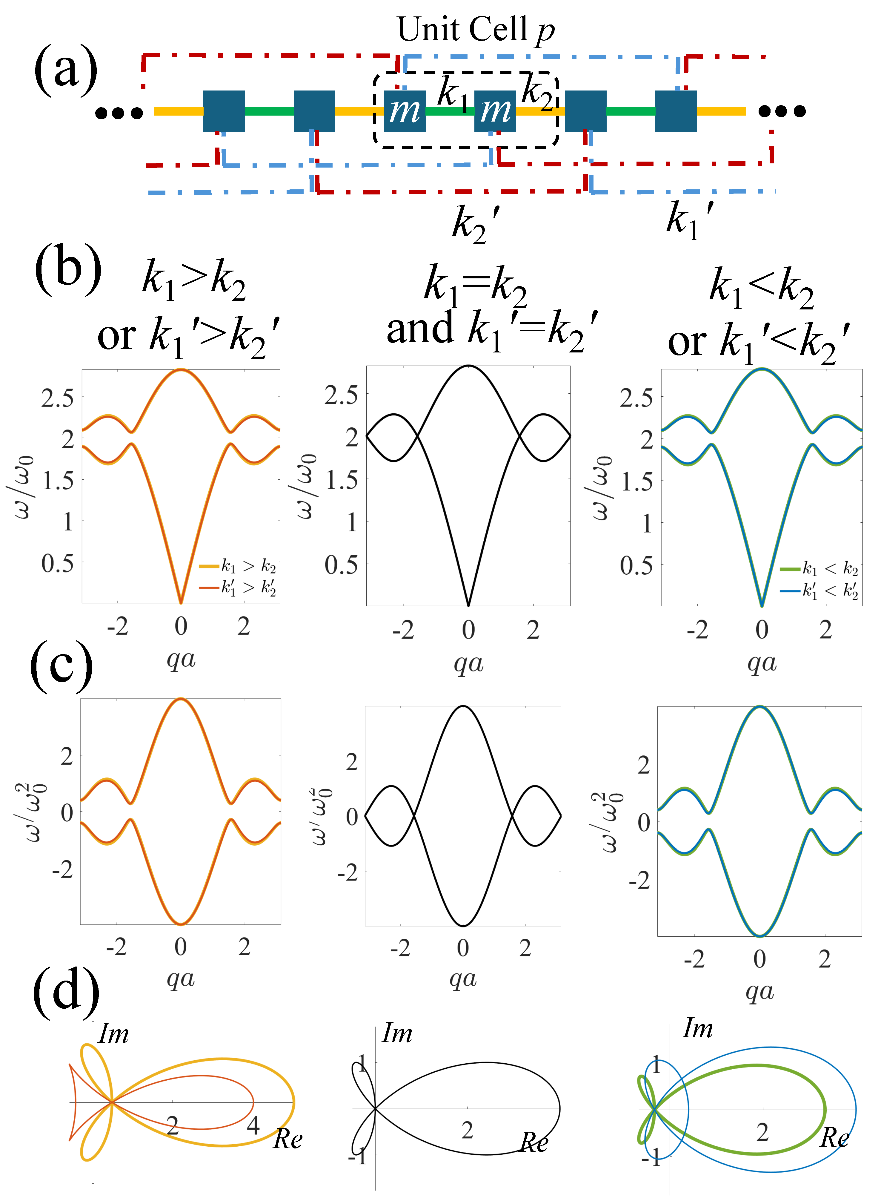
Figure 5.
(a) A finite lattice containing 20 unit cells of identical masses, m, with alternating springs with spring constants (green bars) and (yellow bars) connecting the nearest neighbors, and (blue dashed lines) and (red dashed lines) connecting the third-nearest neighbors. is defined as and . Here, we consider . (b) Normalized eigenfrequencies of the finite lattice in (a). (c) Normalized eigenvalues of the stiffness matrix of (a) after subtracting . (d) 22nd (yellow circles) and 23rd (green triangles) eigenmodes when . (e) Connecting the two ends of the finite lattice to a wall by springs with spring constants , , and to the first, second, and third masses counting from the edges, respectively. (f) Normalized eigenfrequencies of the finite lattice in (e). (g) Normalized eigenvalues of the stiffness matrix of (e) after subtracting . (h) 20th (yellow circles) and 21st (green triangles) eigenmodes when .
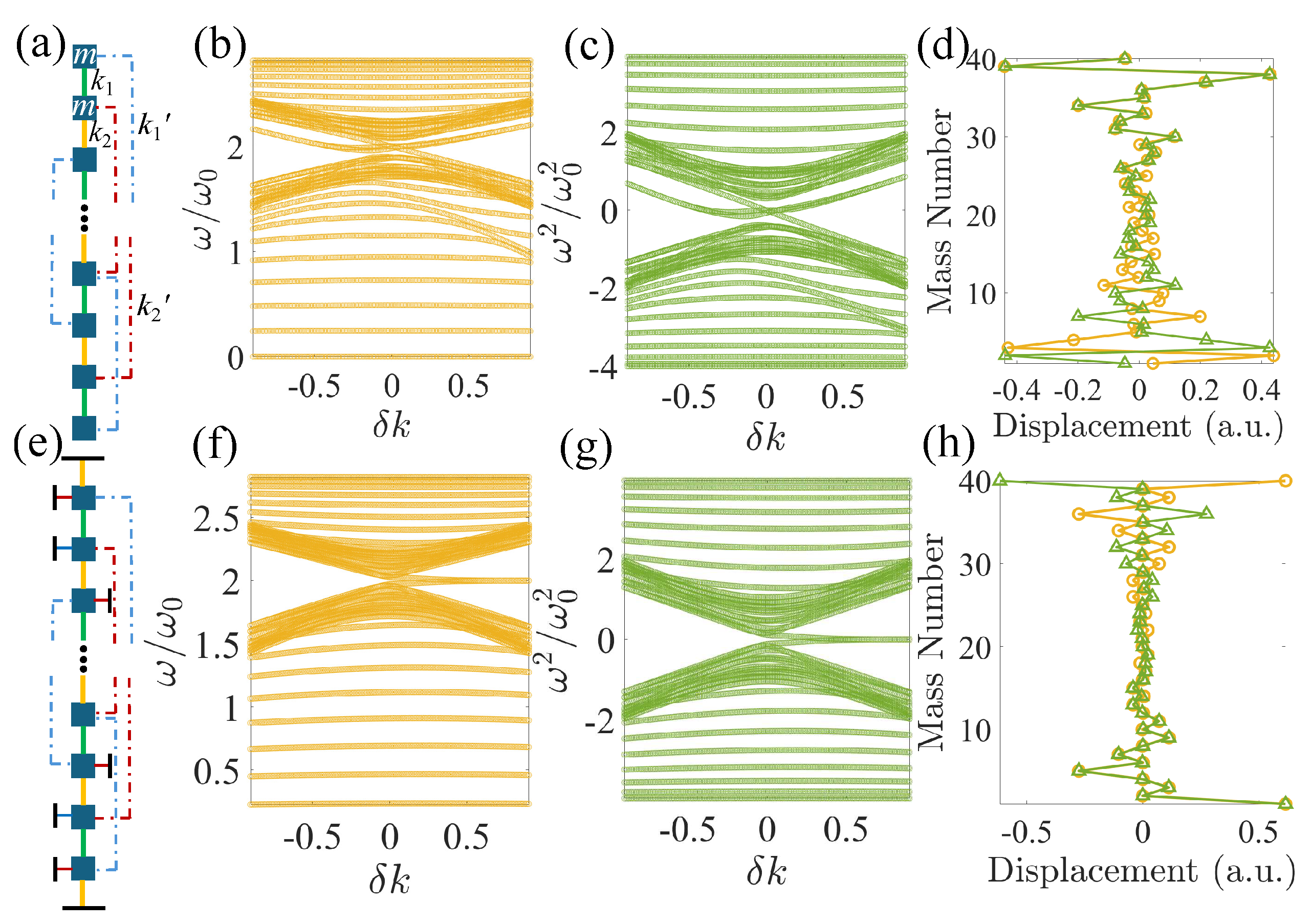
Figure 6.
(a) Normalized eigenfrequencies of the finite lattice in Figure 5(a) with and and . (b) Normalized eigenvalues of the stiffness matrix from the same setup as in (a) after subtracting . (c) and (d) 20-23rd mode shapes (yellow circles, green triangles, blue squares, and red crosses, respectively) when (c) (only 20th and 21st modes are shown) and (d) . (e) Normalized eigenfrequencies of the finite lattice in Figure 5(e) with and and . (f) Normalized eigenvalues of the stiffness matrix from the same setup as (e) after subtracting . (g) and (h) 20-23rd mode shapes (yellow circles, green triangles, blue squares, and red crosses, respectively) when (c) (only 20th and 21st modes are shown) and (d) .
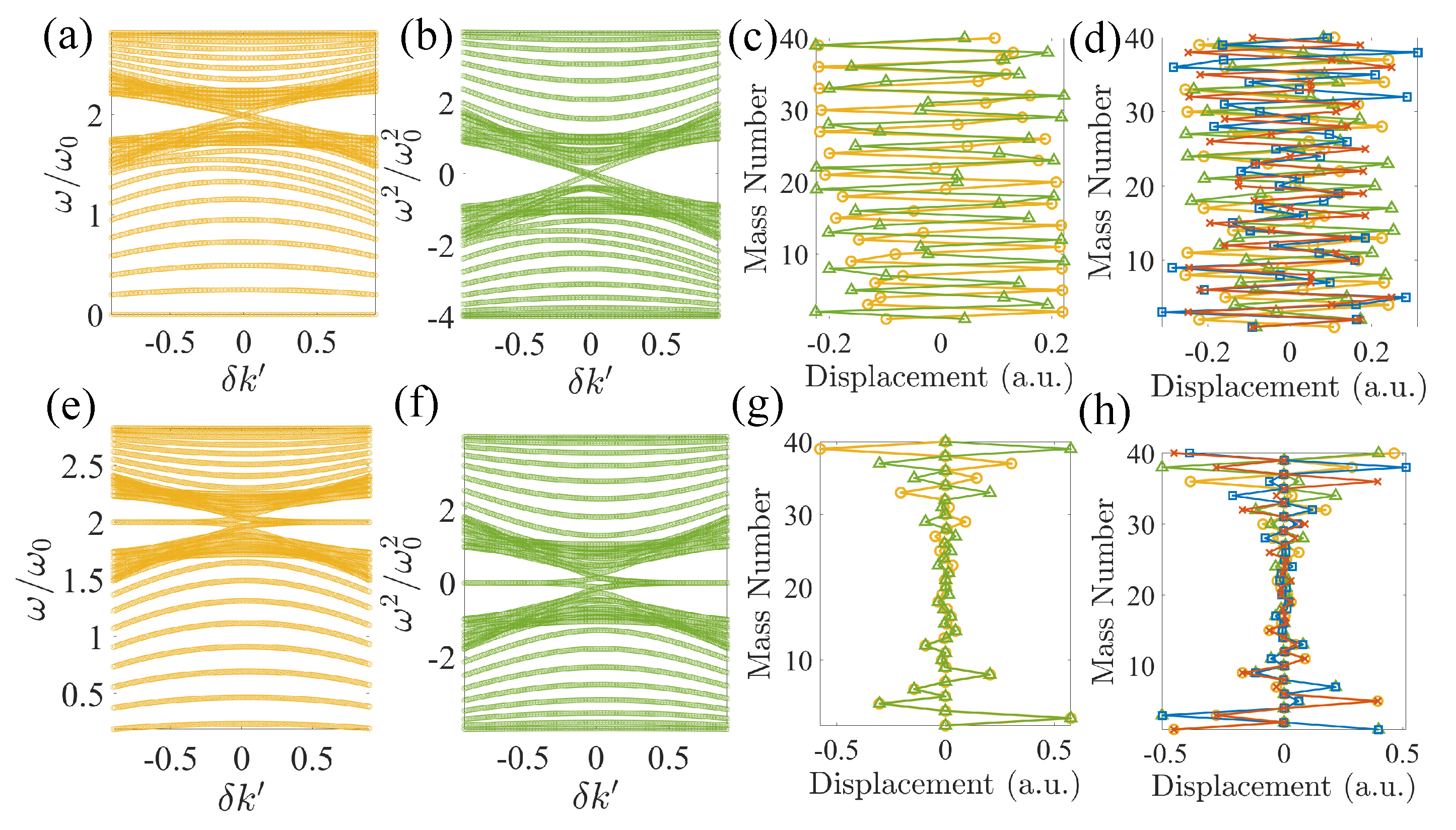
Figure 7.
(a) An infinite lattice with a supercell containing 101 identical masses, m, with alternating nearest neighbor springs with spring constants (green bars) and (yellow bars) ( and ), and third-nearest neighbor springs (blue dashed lines) and (red dashed lines) ( and ). A domain wall is formed at the central mass, about which connected is on both sides. The two masses about the domain wall are connected by . (b) Normalized eigenfrequencies of the finite lattice in (a) when . (c) Normalized eigenvalues of the stiffness matrix of (a) when after subtracting . (d) and (e) 50th to 52nd modes shown as green triangles, yellow circles, and blue squares, respectively, when (d) and (e) . (f) Normalized eigenfrequencies of the finite lattice in (a) when . (g) Normalized eigenvalues of the stiffness matrix of (a) when after subtracting . (h) and (j) 51st and 52nd modes shown as green triangles and yellow circles, respectively, when (h) and (j) .
Disclaimer/Publisher’s Note: The statements, opinions and data contained in all publications are solely those of the individual author(s) and contributor(s) and not of MDPI and/or the editor(s). MDPI and/or the editor(s) disclaim responsibility for any injury to people or property resulting from any ideas, methods, instructions or products referred to in the content. |
© 2024 by the authors. Licensee MDPI, Basel, Switzerland. This article is an open access article distributed under the terms and conditions of the Creative Commons Attribution (CC BY) license (http://creativecommons.org/licenses/by/4.0/).
Copyright: This open access article is published under a Creative Commons CC BY 4.0 license, which permit the free download, distribution, and reuse, provided that the author and preprint are cited in any reuse.


