

Submitted:
25 December 2023
Posted:
26 December 2023
You are already at the latest version
Abstract
In the paper the experimental methodology for the single-crystal circular plate deformation measurement and subsequent procedure for mechanical properties quantitation are developed. The procedure is based on a new numerical-analytical solution of nonlinear boundary-value problem for finite deformations of a circular anisotropic plate. Using the developed method, a study of the deformation of single-crystal circular plates formed on the basis of a silicon-on-insulator structure was carried out. The values of residual stresses are determined and it is shown that the presence of these stresses increases the flexural rigidity of the plate in several times.
Keywords:
micro/nanoelectromechanical system (MEMS/NEMS)
; membrane
; crystalline anisotropy
; single-crystal material
; silicon-on-insulator (SOI)
; deformation
1. Introduction
Nowadays, silicon membrane technology is of a great interest for modern electronics, since it opens the way for the creation of sensitive elements and supporting structures of a number of promising micro/nanoelectromechanical system (MEMS/NEMS)-based devices, such as accelerometers [1,2], pressure sensors [3,4], gas flow meters [5], microbolometers [6,7], digital micromirrors [8,9], resonators [10], microactuators [11], etc. The main task of this technology is to fabricate high-quality thin-film membranes with specified thermo-mechanical properties that ensure appropriate operating characteristics of MEMS/NEMS devices, which, depending on its purpose, is achieved by using various methods: 1) the formation of stress-compensated (or stress-free) multilayer films for thermal sensors by combining materials with compressive (SiO2, TEOS) and tensile (Si3N4, Fe65Co35) stress [5,12,13], 2) selection of layer materials in optical and infrared (IR) membrane sensors with effective absorption of radiation in a given wavelength range [14,15], 3) fabrication of ultrathin extreme ultraviolet (EUV) transparent pellicles to protect the photomask from various contaminants [16], 4) synthesis of new compositions of highly reflective multilayer X-ray mirrors with a roughness below 1 nm [17], 5) use of silicon-on-insulator (SOI) structures with a functional layer based on single-crystalline highly-doped silicon (Si) as a field-emission electrode material in nanoscale vacuum channel transistors [18] or as a thermocouple material with an increased Seebeck coefficient in microbolometer IR detector arrays [19], etc.
To implement the above task in all the described methods, it is important to know the laws of evolution of mechanical stresses in the membrane structure depending on the conditions of its formation - technological regimes (operation temperature, growth rate, elemental composition, etc.), history of the fabrication and mechanical properties of the underlying layers, as well as the physical parameters of the crystalline substrate [20,21,22]. In particular, one of these parameters that influences the residual mechanical stresses and the resulting deformation of the membrane under the action of an applied external (mechanical or electromagnetic) force is the crystallographic orientation of the substrate or its crystalline anisotropy. As applied to SOI structures, this parameter not only specifies the mechanical behaviour of single-crystal Si membranes [23], but also determines the functional (thermal and electrical) properties of the electronic components integrated in the membrane device layer [24]. At the same time, there is no analytical model that allows one to reliably predict the effect of crystalline anisotropy of the substrate on the nature of the distribution of internal mechanical fields in the presence of an applied load.
In the present work, we compare the bending profiles of a single-crystal Si membrane of the SOI structure with crystallographic orientation <100>, which are measured in the experiment at various pressure (in the range from 0 to about 300 kPa) and calculated within the framework of non-linear elasticity theory based on iterative solving three-dimensional Lamé equations with non-linear RHS part. Based on this comparison, the great influence of the initial tension in the single-crystal Si membrane on the deformation of the SOI substrate were established.
2. Materials and methods
2.1. Design and technology of the fabrication of SOI-based thin-film Si membranes
A description of the process flow for the fabrication of a single-crystalline silicon (Si) membrane formed on the basis of a silicon-on-insulator (SOI) structure is presented in Figure 1. The initial structure of the SOI substrate (Figure 1a) consists of the following sequence of layers: top (thin) Si layer with a thickness of 2.86 µm, from which a single-crystal membrane is formed, an intermediate dielectric layer of SiO2 with a thickness of 1 µm, and the bottom (thick) Si layer, the thickness of which is in accordance with the total SOI thickness (608 µm) is 604.14 µm.
In the first step of the fabrication process, a mask is formed on the SOI substrate for etching silicon (Si) to a depth comparable to its thickness (608 µm). A photoresist layer with a thickness of several microns is etched off before etching of a SOI substrate with a thickness of 608 µm occurs, and therefore the standard photoresist layer is replaced by an aluminum (Al) layer, which, compared to the standard photoresist, has a greater selectivity of etching to silicon (Si). Thus, a layer of aluminum (Al) with a thickness of 1.1 µm is formed on the reverse side of the SOI substrate by magnetron sputtering technique, after which it is covered with a polymethyl methacrylate (PMMA) photoresist layer using the spin coating method for subsequent contact photolithography (Figure 1b). The photoresist is then exposed through a mask and developed, after which the aluminum (Al) layer in the exposed area is removed by wet etching in a specially selected etchant consisting of 80% H3PO4, 5% HNO3, 5% HAc and 10% H2O (Figure 1c). After removing the photoresist layer, the next step is plasma-chemical etching of Si from the back side of the SOI substrate (Bosch process), where a layer of silicon oxide (SiO2) serves as a etching-stop layer. The last step is to remove the remaining SiO2 layer in hydrofluoric acid (HF) vapor, thereby freeing the single-crystalline silicon (Si) membrane (Figure 1d). To fabricate a single-crystalline Si membrane with a round shape with a thickness of 2.86 µm and a diameter of 0.936 mm, a BSOI 600-1.5-7 substrate with a diameter of 150 mm and crystallographic orientation (100) was used. To experimentally demonstrate the change in the profile of a thin-film Si membrane under the influence of applied external pressure, several of the most characteristic representatives were selected from the original SOI substrate with membrane structures manufactured according to the fabrication process flow (see Fig. 1).
2.2. Experimental setup for measuring the profile of fabricated Si membranes at non-zero pressure
The experimental setup for measuring the mechanical properties of thin-film structures, which is illustrated in Figure 2, consists of the following components: a pipe line with the ability to supply air or any other gas with a pressure in the range of up to 7 atm., a receiver cylinder with an analog pressure gauge, a filter regulator MC104- D00, pressure regulator ER104-5PAP, Arduino Mega 2560 board, personal computer (PC), Veeco Wyko NT9300 profilometer, vibration isolation platform.
The receiver cylinder acts as a buffer tank to smooth out gas pressure differences and ensure the overall stability of the measuring system. The supplied air enters the filter regulator MC104-D00 with a filter element made of high-density polyethylene (HDPE) membrane with a filtration fineness of 25 µm according to the ISO 8573-1:2010 standard. The pressure regulator is responsible for maintaining a constant and controlled level of excess pressure. Several pressure gauges are located at various points on the bench to provide real-time monitoring of pressure levels. There are also built-in safety valves to automatically relieve excess pressure in the event of a diaphragm rupture. Software for the Arduino Mega 2560 board provides control of the pressure applied to the membrane. The accuracy of overpressure supply is 0.01 atm. The accuracy of measuring the relief (deflection) of the membrane along the vertical axis is no worse than 5 nm. A schematic diagram of the experimental setup is presented in Figure 3.
Using the experimental setup described above, the deflection profile of the fabricated silicon (Si) membranes with a diameter of 0.936 mm was measured. Figure 4 illustrates the results of measurements of the shape of two samples of fabricated single-crystal Si membrane under applied pressure, obtained using the experimental setup shown in Figure 2. As can be seen from the figure, the vertical coordinate of the membrane profile in the center changes nonlinearly with pressure, while the profile remains symmetrical relative to the center.
3. Theoretical statement of the problem
In this part we construct a closed solution of boundary value problem for linear elastic anisotropic circular plate. We will seek the solution in the class of square-integrable vector-functions, defined over the domain, occupied by the plate. It is known that under certain boundary conditions the separation of variables can be used. We’ll take advantage of this opportunity. To this end the specific boundary conditions of roller contact type must be specified on the lateral surface of the plate. This limitation does not seem burdensome, since it corresponds to the conditions under which the experiment is provided (as will be shown below, they can be taken into account in the model very accurately by choosing a specific distribution of volumetric force). These considerations allow the solution to be represented in the form of an expansion over a system of vector-valued eigenfunctions, generated by the auxiliary problem of Bessel type.
First let’s make some notes about the representation of coordinates and fields. We will represent all kinematic fields and stresses in cylindrical coordinates :
and corresponding local physical bases :
Here denote standard rectangular coordinates, while stand for the elements of Cartesian orthonormal basis. Since the problem at the first stage is considered in a linear formulation (geometric non-linearity will be taken into account in section 6), we will not distinguish the reference and actual shapes of the body, assuming that both coincide with the region
Due to the peculiarities of the experimental data, we will need to study only axisymmetric deformation. In this regard, we define the general representation of the desired displacement field as
where are the functions to be defined:
The design diagram of the plate is shown in Figure 5.
Let’s move on to the discussion of boundary conditions that meet the method of sample fixing in an experiment. Suppose that the lateral boundary of the cylindrical plate is free from tangential stresses and fixed in radial direction. From the viewpoint of structural mechanics these conditions correspond to ”roller contact” of cylindrical part of the plate boundary with absolutely rigid tube without friction. Some restrictions, that has to be taken into account in conditions on the cylindrical part of the boundary, give complete freedom to choose conditions on the flat part, i.e., on the bases of the cylinder (plate face surfaces). In order to reproduce the experimental conditions, we assume that the bases are not fixed and believe that a volumetric distributed force is applied on the interior of the cylinder. Note that, under given above boundary conditions, the plate can move as a rigid body along its axis. In order to exclude such motion, we assume that, besides axial symmetry, the external loads (both surface and volumetric) are self-balanced, that is, their net force and net moment vanish, i.e.
We especially note one of the particular distribution of volumetric force
Here is Heaviside step function. The parameter a is chosen to be sufficiently close to the plate radius. These distributions correspond to an uniformly distributed volume force in the main area of the plate and distributed reaction in a narrow annular area. The latter integrally characterises the reaction of the support in experimental setup. It should be noted that, on the one hand, this formalization allows to remain within the framework of the boundary conditions discussed above. On the other hand, because it’s actually very difficult to experimentally identify in detail the specific distributions of reaction at the cylindrical part of sample boundary, they are still considered in integral form.
Now we turn to the formulation of the constitutive equation for an transversely isotropic material. Firstly note, that in the case of axial symmetry infinitesimal deformations are determined by the formulae
These deformations cause stresses, defined by the fourth-rank elasticity tensor :
which in the case of a transversely isotropic material can be written in the Voigt form as the following matrix :
Thus one can obtain relation (3) in component form:
where are material constants, which characterise transverse isotropy in most general form. The only axis of such anisotropy is supposed to be oriented along the axis of the cylindrical plate. For the convenience of subsequent computational analysis, we present the anisotropic elastic moduli as the result of a continuous morphism of isotropic elastic one:
where are Lamé material constants of polycrystalline material, which correspond to those of crystalline material by Voigt formulae [25]:
Substituting (2), (3) into the equilibrium equations
we arrive at the system of partial differential equations:
In light of the above the boundary conditions can be stated as follows:
The equations (6) and boundary conditions (7) together with requirement of self-balance (1) gives linear statement for the boundary-valued problem under consideration.
It is convenient to carry out further calculations in dimensionless variables (in the next line they are denoted with twiddle), which are related to their dimensional counterparts by formulae:
In what follows, we will omit the tilde sign, since the question of which formulation is used, dimensional or dimensionless, is easy to answer based on the context.
4. Solution of the linear boundary-value problem
Before proceeding to the solution, we note that so formulated problem allows for complete separation of spatial variables. Indeed, if one represent sought variables u, w in the form of multiplicative decomposition
that meet the conditions
where is an arbitrary constant, then the system of homogeneous equation, defined by LHS of (6) can be written in the form
Here are constants of separation [26], and the prime means differentiation with respect to the variable on which a specific function depends. Actually, these constants turn out to be equal, which is easy to see from the relations, that can be obtained by differentiation of equations (8):
Taking them into account, from (9) one gets
Therefore, a homogeneous system of partial differential equations splits into two independent systems of ordinary differential equations
Separating the variables in equations is only half a matter. To complete the matter, it is also necessary to separate the variables in the boundary conditions. But this is where the considerations, discussed above for the cylindrical part of the boundary, come in handy. Substituting (4) into LHS of relations (7) one obtains:
Thus, we arrive at two independent boundary-value problems containing only ordinary differential equations (ODE). It is this fact, that allows us to further construct representations of the solution in terms of known elementary and special functions, since all of them are solutions of corresponding ODE’s.
Let’s now start constructing the solution of (10) – (13) itself. First, consider the auxiliary problem (10), (12). Note that, because the corresponding differential operator is self-conjugate, it can be classified as Sturm–Liouville problem on the interval [27]. It follows that all it`s non-trivial solutions constitute a basis in Hilbert space of vector-valued functions over this interval. The solution of the equations (10) (for ) can be given in the form of combinations of Bessel functions:
where and are arbitrary constants, are Bessel functions of the first and second kind correspondingly [28]. Keeping in mind that the sought displacement functions has to be bounded at the pole (), we set constants , equal to zero. The two remaining boundary conditions (12) will be satisfied if any root of the transcendental equation
is taken as . In fact, each such a value is two-fold eigenvalue of the Sturm-Liouville problem, which corresponds to the two-dimensional eigensubspace. The bases in each subspace can be chosen by setting the constants equal to and . It remains only to note that in the special case the solution to the boundary value problem has the form . Thus the eigenfunctions can be defined as countable sequence
where
and any square-integrable vector-function can be represent (in weak form) as decomposition
with suitable sequence of Fourier coefficients . To simplify calculations, it is advisable to use normalized eigenfunctions
The decomposition procedure can be formalized with orthogonal projectors onto eigensubspaces, represented in the following form:
Now any square-integrable function can be represented by a sequence of Fourier coefficients, and vice versa, from the sequence of Fourier coefficients a vector function can be reconstructed (in the weak sense)
Here denotes the space of square summable sequences, while is the space of quadratically integrable (with weight r) two-component vector-functions, and stands for the result of successive mutual mappings between these spaces, which may differ from the original on a set of measure zero [27].
Note that direct numerical computation for a long sequences of transcendental equation roots gives rise to a well-known computational problem (in a view of possible missing roots or incorrect determination of their multiplicity). In application to the problem under consideration it can be easily solved if one applies the asymptotic approximation for :
The result of the action of projection operators (14) on the right-hand sides of the equations (6) will be denoted by the symbols
For further analysis, we will need projections of two special cases of distributions of volumetric forces relative to the radial coordinate, namely
- stepwise self-balanced distribution taking a unit value on the interval and a constant value of the opposite sign on the interval , i.e.
- self-balanced distribution (see (1)), taking a unit value on the interval and a constant value of the opposite sign on the interval , i.e.
The formulations of such distributions and the result of the action of projectors on them are given below:
Passing to the limit in these relations, and taking into account the equality
where is a zero of , one can obtain the following expressions for projections, valid for the case :
This corresponds to the case when the reactive body forces are distributed in an infinitely thin boundary ring (and can be formally represented in terms of Dirac delta functions).
Using constructed above orthonormal basis, one can represent the sought displacement functions in the form of expansions
where , , are Fourier coefficients which themselves are functions, but of another spatial variable z. To find these coefficients, one has to substitute the formal expansion (16) into equations (6), boundary conditions (7) and then apply projectors (14) to the left and right sides of the resulting functional equations. This results in countable sequence of independent ordinary differential equations (with respect to z),
and two-point boundary conditions
As above, we will separately consider the case
One can see that something is wrong with this boundary-value problem. Indeed, the solution of differential equation (19) can be obtained in the form
but from the boundary conditions it is impossible to determine the constant . On the other hand, differentiating the resulting solution, we find
Therefore, to satisfy first boundary condition, one should set and the second boundary condition will be satisfied only if
It easy to see that the condition for the existence of a solution is equivalent to the requirement for external fields to be self-balanced.
All we have to do is to obtain solutions for two-point boundary value problems with respect to expansion coefficients. These boundary-value problems are of the same type and are determined by ordinary differential equations with constant coefficients. To this end we firstly get the general solution of differential equation (17) in the form (to shorten the notation, we will omit the index n):
Here stands for the matrix containing fundamental system of solutions for homogeneous counterpart of equation (17):
where A, B are the roots of corresponding characteristic equation,
and denotes particular solution, obtained with Lagrange method:
Constants of integration, defined by the expression in parentheses (20), are chosen in such a way that the boundary conditions (18) are satisfied. They are given by the following expressions
In the above expressions, the following notation was used for abbreviation:
and
In the case when the density of volumetric force does not depend on z (and equal to ), the particular solution (23) takes the form:
Corresponding values for constants of integration are
Another important case, which will be used in section 6, corresponds to the unit distribution on interval , i.e.
It should be noted that in the case of an isotropic material (), the values of the roots (22) of the characteristic equation coincide, , and to construct a solution, instead of the fundamental matrix (21), one should use the matrix, which is obtained from the latter by passing to the limit and contains the ODE associated solutions:
where (, are the Voigt average moduli (5)). All other relations are obtained similarly by passing to the limit.
5. Algorithmic solution implementation
From the above constructions it follows that the desired solution for an arbitrary right-hand side can be represented by the series
where and are constants, while , are functions on z (they become constant in the case of homogeneous volumetric force distribution with respect to z). Explicit expressions for these quantities can be obtained from the above formulas. Their form depends on the result of integration (23), (14) and can be very cumbersome (due to known difficulties of integration in a closed form). But to implement a computational algorithm, the use of closed analytical expressions at each stage seems to be superfluous. In order to use the simple solution obtained above for a constant density of volumetric forces on a rectangular support, we represent arbitrary RHS in (6) as piecewise constant vector-function
where denotes the characteristic function
of rectangular domain
and are numerical two-component vectors, which values determine the levels of the RHS components in corresponding domain. Using the solutions (24), (15) one can find the values for each individual partial load, identified with pair numbers , as follows:
Since at this stage the problem is solved in a linear formulation, it is possible to use the superposition of solutions to determine the response on the full field of body forces. Thus the desired solution of the problem (6) can be presented in the same form (25) with following parameters
To implement the computational algorithm, it is convenient to pre-calculate solutions for partial unit volumetric forces, thereby determining the discrete analogue of the Green’s function. This algorithm is a computational implementation of the linear operator inverse to the operator, generated by differential equations (6) and boundary conditions (7). This linear operator will be further denoted by the symbol .
6. Geometric non-linearity
To take into account the geometric non-linearity, one has to treat stresses, introduced previously in the framework of linear elasticity, as second Piola – Kirchhoff stresses . This allows formal expression for constitutive law, similar to (3)
where is Green – Saint-Venant strain tensor
is infinitesimal strain tensor, defined in (2), denotes displacement gradient and stands for the forth rank tensor of linear elastic moduli, used in (3). Understanding that this is only the one of the possible, and probably not the best, type of constitutive law in non-linear elasticity, we use it to take advantage of the previously constructed linear solution.
Let us now proceed to the construction of an iterative algorithm for determining displacements taking into account geometric non-linearity. The starting point will be the equilibrium equation formulated in reference coordinates with respect to second Piola-Kirchhoff tensor :
Bearing in mind the linearity of the divergence operator and taking into account the additive expansion (26), we rewrite the equation in the form
Now we can implement a fixed-point iteration process:
Here
At each step of the iterative process, it is necessary to solve a linear problem (6), (7) for the distribution of volumetric forces specified by the relation (27). For this purpose, we use the analytical solution, obtained above, which determines the linear (inverse) operator . Using it, we get the following recurrent sequence:
This sequence converges quickly enough, if at each step the right-hand side of the equation (28) sligtly differs from . At the same time, it is the cases when the nonlinear term manifests itself significantly that are most interesting. To overcome the divergence problem, it is proposed to use regularization of the iterative process, the idea of which is similar to the Fejér summation method (with arithmetic means). In this case, at each step we calculate
where is the regularizer of the iterative process, using the ”memory” of all previous iterations and, thereby, creating ”computational viscosity” in the algorithm:
Sequence of weight factors specifies the ”memory” depth. If
then the regularizer does not make any corrections to the iterations, but if , then the regularizer takes into account the entire history of the iterative process and performs the best smoothing of its variability. Of course, in this case more iterations are required. Choice of a specific type of sequence of weighting factors depends on the contribution of nonlinear terms to the solution and, ultimately, on the ratio of the expected deflection to the characteristic size of the plate.
In order to take into account the initial tension, one should replace displacements with in the above formulas. Here and defines predetermined homogeneous initial stretching in radial direction.
7. Sensitivity of proposed theoretical model on the mechanical parameters
Before identification of mechanical characteristics upon the experimental data, we analyse the sensitivity of proposed theoretical model on the parameters, which characterise the elastic properties of the material, and on the loading intensity.
Above solutions were constructed for both isotropic and anisotropic cases. Moreover, anisotropic elastic moduli can be continuously transformed into isotropic counterparts, when the anisotropy factor t changes from 1 to 0 (see (4)). Now, to estimate the impact of anisotropy factor, we find the dependence on t of plate displacements under a unit distributed volumetric force. Recall that the case corresponds to a full account of anisotropy, at we have a partial account, and the case corresponds to a completely isotropic material which elastic moduli are obtained by Voigt averaging (5). For test calculations, we deliberately significantly increased the thickness of the plate to 20% of the radius. This allows, firstly, to illustrate the impact of the anisotropy factor more clearly, and secondly, to present the calculation results on a natural two-dimensional picture. Keeping in mind the linearity of the model, we perform calculations for a unit intensity of body forces, and present results in dimensionless form.
The following values of elastic moduli for crystalline silicon were used in the calculations:

Table 1.
Elastic moduli for crystalline silicon, GPa
| 186 | 64 | 64 | 80 | 186 |
They correspond to the following Voigt-averaged moduli for polycrystallite
In Figure 6 the graphs that illustrate such dependencies are given. In Figure 6 one can find the difference between distorted mesh with and without accounting of anisotropy, while Figure 6 demonstrates the distinction in displacements of the bottom of the plate. It can be seen that the account of anisotropy does not have a significant effect on the theoretical flexural rigidity of the plate: the largest difference in displacements does not exceed 8.7%.
To assess the impact of the anisotropy factor on the stress state, the stress values were found at the lower central point (point A in Figure 5) and at the corner point on the boundary (point B in Figure 5). The results are shown in the Table 2. The tensions found with account of anisotropy and without it differ by no more than 8%.
Much more significant is the influence of geometric nonlinearity caused by an increase in tensile stresses on the cylindrical part of the boundary when the plate is deformed. To illustrate this, consider the dependence of the displacements of the center of the plate bottom with increasing intensity of a uniformly distributed pressure on the plate top. We will change the load intensity in the range kPa. The dependence over the entire range is shown in Figure 7. It clearly has non-linear nature. At the same time, in certain intervals it can be interpreted with sufficient accuracy as linear. The first, and most natural, such interval is rather short, it is kPa. It characterizes deformation range, in which all non-linear effects are negligibly small. Corresponding pressure-displacement curve is shown on Figure 7 in purple shading. Already at the next interval, kPa, nonlinear effects manifest themselves significantly. This can be seen on the pressure-displacement curve on Figure 7 (in green shading), where the linear dependence that continues the dependence from previous interval is shown in black. For comparison the tangent to the pressure-displacement curve (at the middle of the interval) is shown in red. Keeping in mind the concept of tangent modulus used in elasticity theory, we can interpret this tangent as some effective stiffness. It must only be borne in mind that such effective stiffness, due to the fact that it depends on the tension on boundary, reflects a property of the structure and not of the material alone. The dependence in the next interval kPa is most nonlinear and is shown in blue shading on Figure 7 Just as before, the black line represents the continuation of the linear relationship, and the tangent in the middle of the interval is shown in red. It should be noted that, unlike the previous intervals, the displacement computed within the linear theory differs from the displacements calculated with account of geometric non-linearity by several times. The slope of the black and red lines are also significantly different, which means that the effective stiffness varies considerably from what can be calculated in the linear approximation. The last interval is the longest, kPa (Figure 7). Displacements calculated within the framework of linear theory differ by an order of magnitude from those calculated taking into account geometric non-linearity. At the same time, the very dependence of displacements on pressure in this interval is close to linear, as can be seen from its comparison with the tangent (red straight line). One just needs to keep in mind that such a linear dependence does not characterize the linearity of the elastic properties of the material, but the linearity of the rigidity of the structure in this load range.
The increase in the effective stiffness of the plate due to nonlinear effects can be quantitatively assessed by comparing the slope of tangents at midpoints of different intervals of the pressure-displacement curve. Their values are given in Table 3. Note that the minimal and maximal slope differ by a factor of 32.
Now consider the effect of the initial tension in the radial direction on the effective stiffness of the plate. For different values of the initial tension in the radial direction, we will apply the same load 100 kPa to the upper surface of the plate. Displacements of the bottom surface are shown on Figure 8. Note that by changing the initial tension one can change the maximal deflections by an order of magnitude.
Therefore, the preliminary analysis of the mathematical model, applied to the plate tested in the experiment, allows us to state the following:
- Displacements weakly depend on whether or not the anisotropy factor is taken into account.
- Geometric nonlinearity can be neglected at a load of no more than 100 Pa. At pressures exceeding this value, the influence of geometric nonlinearity increases dramatically.
- Displacements can vary by more than an order of magnitude depending on the initial in-plane tension.
8. Identification of experimental data
Now let’s move on to the analysis of experimental data. Two series of experiments were carried out, during which the profiles of the plate deformed by uniform pressure were determined. The intensity of the pressure varies from 20 kPa up to 300 kPa with increment 10 kPa. The difference between the profile measured at the n-th step and the profile measured before loading determines the displacement along the z axis of the top surface of the plate. The experimentally determined displacements in the first series of measurements are shown in Figure 9, and in the second in Figure 10, where the distribution of measured values are shown as polygons of alternating colours.
The displacements of the central point are determined by averaging over a centered strip of mm wide (one tenth of the diameter). It is shown in yellow in the pictures. The results of averaging are shown with brown lines and pointed on lateral plane with brown dots. These dots together represent the pressure-displacement curve for the central point of plate bottom (shown in black). Confidence intervals (with 0.95 level) are also shown in brown.
As expected, the dependencies for the displacements of the central points on pressure are close to linear. This, however, does not mean at all that a linear model of an elastic body can be used to interpret the experiment. Based on the preliminary calculations carried out above, we can expect that the pressure-displacement curve corresponds to the last interval, in which the geometrical non-linearity has strong impact.
At this stage, we have insufficient experimental data to simultaneously identify elastic moduli and tension, but if we assume the elastic moduli are known, then tension can be identified. To this end we compute the values of central point displacements for the values of tension that corresponds to radial displacements of the boundary in the range and pressure varies in the range kPa. The resulting dependence is shown on Figure 11 as yellow surface. Then we take the experimental dependence for central point displacements from two series and compute the standard deviation of the experimental data from theoretical estimation for varying value of tension. All that remains is to find such tension values, and for which the standard deviation becomes minimal. These values are
- For the first series of experimental data the stretching in radial direction is . The corresponding radial component of stresses is MPa.
- For the second series of experimental data the stretching in radial direction is . The corresponding radial component of stresses is MPa.
These values correspond to certain sections of the surface that represents the theoretical distribution for displacements, at the intersection with which the experimental distributions in the form of blue polygons are shown on Figure 11
For a more detailed comparison of theoretical and experimental values, we depict these sections on separate graphs in Figure 12 One can also see on these graphs confidence intervals computed upon experimental data. The slight difference between the theoretical distributions and experimental data can be explained by the fact that the theoretical model takes into account geometric non-linearity, while the constitutive law is still assumed to be linear. It is likely that the use of more suitable hyperelastic potentials will allow us to construct a more accurate theoretical model. We hope that such generalizations will be obtained in subsequent works.
9. Comparison of the proposed mathematical model with standard formulas
Finally, we compare the proposed mathematical model with standard formulas usually used to identify experiments on the deformation of thin films. First we note that three classes of such formulas can be distinguished. The first class includes formulas obtained from solutions of boundary value problems on the bending of elastic plates within the framework of a theory of the Kirchhoff – Love type. Formulas of the second class are obtained from numerical solutions of the Föppl – von Kármán equations, obtained by the Galerkin method. In this case, as a rule, a one-term approximation is used, which corresponds to the assumption that the curved shape of the plate is spherical. The third class contains formulas obtained empirically. For a uniformly loaded circular plate of isotropic material, these three types are represented by the formulae, given in Table 4.
Note that the last, empirical, formula is a formal combination of two different analytical relationships, the first of which determines the bending of the membrane from the solution of the Poisson equation, and the second represents the first term of the Galerkin solution to the bending equation of flexible plates.
To compare the proposed solution with the mentioned approximations, a series of calculations were made for a sequence of thicknesses and pressures. Their values and the results are shown in the Table 5. In this table one can see the vertical displacements of the plate bottom, computed with proposed model, v.s. deflections calculated in the framework of corresponding plate theory with formulae, given in first two rows of Table 4. Differences are shown by shading. From the analysis of the results it is clear that the theory of Kirchhoff-Love plates gives a good approximation for small deflections and thicknesses, while the spherical approximation of the solution to the Föppl – von Kármán equations gives a small error for significant deflections and also small thicknesses. In general, these approximations have a rather narrow range of application. At the same time, they are often used to identify the results of experiments, and therefore we decided to calculate from them the values of theoretically expected displacements of the midpoint of the plate in order to assess the possible error introduced by such approximate calculations. The results are shown in Table 6. The maximal displacements of the plate were compared at a pressure of 150 kPa. The first two columns show the displacements and initial tensions found above from the experimental results. The third column shows the theoretical values of maximal displacements calculated using the proposed model. The last two columns show displacements found using simplified formulae. Errors calculated relative to experimental data are given in parentheses. It can be seen that the errors of the approximate formulas exceed the accuracy required to identify the anisotropy factors. At the same time, we note that the empirical formula (into which, however, we substituted the initial tension found using the proposed method) for large pressure gives rather accurate result. This is apparently due to the fact that at large deflections the membrane stress-strain state prevails and is well determined from the classical Poisson equation (recall that the first part of the empirical formula is precisely the solution to the corresponding Poisson equation).
10. Conclusions
The following conclusions can be drawn from the work.
1. The account of the anisotropic moduli of the crystal in the analysis of single-crystal plate stress-strained state leads to theoretical corrections about 10%. In this regard, to analyze anisotropic properties, the experimental error should be less than 10%. At this level of errors, in the identification of the experimental results the approximation formulas either cannot be used at all, or they can be used in narrow ranges of mechanical parameters. On the contrary, the proposed numerical-analytical solution can be used for the identification in a wide range of parameters.
2. The initial tension has a great influence on the effective flexural rigidity of the plate. For single-crystal circular plates formed on the basis of a silicon-on-insulator structure the initial stresses change the rigidity in several times.
3. The proposed experimental technique makes it possible to quite accurately quantify the initial stresses and, taking them into account, the effective flexural rigidity.
The mathematical modelling and analysis of experimental data allows us to clarify the questions that experimenters need to answer in subsequent works. First, a series of mechanical tests should be carried out in the range of almost linear deformations, from which the anisotropic elastic moduli can be directly determined, independent of the effects caused by geometric non-linearity. To this end, if one use plates of the same thickness as in the experiments described above, then the loading steps should be taken on the order of 100 Pa. It may be technically more convenient to use thicker plates, which will allow the pressure increment to be increased. Secondly, a series of experiments should be carried out with a small step of pressure increment, but adding these increments upon a significant pre-load. This will allow one to feel the effects of superimposing small deformations on finite ones and distinguish the impact of geometric non-linearity and possibly physical non-linearity. The last factor is of particular interest for the finite deformations modelling of anisotropic crystals. Thirdly, a series of experiments, similar to those described in present work, should be carried out, but with plates obtained at different deposition temperatures. Changing the manufacturing conditions will affect the initial tensions and, as the analysis in this paper shows, will significantly change the effective flexural stiffness of the plates.
Author Contributions
Conceptualization and methodology, S.L., G.D.; writing—original draft preparation, S.L., A.D., G.D., E.G., I.K., N.D., V.B. All authors have read and agreed to the published version of the manuscript.
Funding
The work was supported by the Ministry of Science and Higher Education of the Russian Federation (State Assignment № FSMR-2023-0014).
Institutional Review Board Statement
Not applicable.
Informed Consent Statement
Not applicable.
Data Availability Statement
The authors confirm that the data supporting the findings of this study are available within the article.
Acknowledgments
The experimental part of the research, devoted to the study of test samples of single-crystal Si membranes, was performed using the equipment of R&D Center «MEMSEC» of National Research University of Electronic Technology (MIET).
Conflicts of Interest
The authors declare no conflict of interest.
Abbreviations
The following abbreviations are used in this manuscript:
| LHS | left-hand side |
| MDPI | Multidisciplinary Digital Publishing Institute |
| RHS | right-hand side |
References
- Zhang, J.; Shi, Y.; Cao, H.; Zhao, S.; Zhao, Y.; Wang, Y.; Zhao, R.; Hou, X.; He, J.; Chou, X. Design and implementation of a novel membrane-island structured MEMS accelerometer with an ultra-high range. IEEE Sensors Journal 2022, 22, 20246–20256. [Google Scholar] [CrossRef]
- Ovodov, A.I.; Demin, G.D.; Djuzhev, N.A.; Makhiboroda, M.A. Optimized design of the MEMS-based three-axis thermal accelerometer for its better performance in a wide measurement range. In Proceedings of the 2019 IEEE Sensors Applications Symposium (SAS), Sophia Antipolis, France, 11-13 March 2019; pp. 1–5. [Google Scholar]
- Xu, M.; Feng, Y.; Han, X.; Ke, X.; Li, G.; Zeng, Y.; Yan, H.; Li, D. Design and fabrication of an absolute pressure MEMS capacitance vacuum sensor based on silicon bonding technology. Vacuum 2021, 186, 110065. [Google Scholar] [CrossRef]
- Demin, G.D.; Djuzhev, N.A.; Pozdnyakov, M.M.; Evsikov, I.D.; Oreshkin, G.I. Simulation of a Sensitive Element of a MEMS-Based Pressure Sensor Operating on The Thermal Detection Principle. In Proceedings of the 2021 IEEE 22nd International Conference of Young Professionals in Electron Devices and Materials (EDM), March 2019; pp. 87–90. [Google Scholar]
- Djuzhev, N.A.; Ryabov, V.T.; Demin, G.D.; Makhiboroda, M.A.; Evsikov, I.D.; Pozdnyakov, M.M.; Bespalov, V.A. Measurement System for Wide-Range Flow Evaluation and Thermal Characterization of MEMS-Based Thermoresistive Flow-Rate Sensors. Sensors and Actuators A Physical 2021, 330, 112832. [Google Scholar] [CrossRef]
- Yu, L.; Guo, Y.; Zhu, H.; Luo, M.; Han, P.; Ji, X. Low-cost microbolometer type infrared detectors. Micromachines 2020, 11, 800. [Google Scholar] [CrossRef] [PubMed]
- Evsikov, I.D.; Demin, G.D.; Djuzhev, N.A.; Fetisov, E.A.; Khafizov, R.Z. TCAD simulation of the etching of the sacrificial layer in the sensitive element of the IR microbolometer array based on the SOI structure. MES 2022, 4, 228–233. [Google Scholar] [CrossRef]
- Chen, S.; Zhang, Y.; Hong, X.; Li, J. Technologies and applications of silicon-based Micro-Optical Electromechanical Systems: a brief review. J. Semicond 2022, 43, 081301. [Google Scholar] [CrossRef]
- Demin, G.D.; Kim, P.P.; Pozdnyakov, M.M.; Filippov, N.A.; Dyuzhev, N.A. Analysis of Electromechanical Deformation of a MEMS Element of a Reflection-Type Dynamic Mask Based on a Torsional Micromirror. In Proceedings of the 2022 IEEE 23rd International Conference of Young Professionals in Electron Devices and Materials (EDM), June 2022; pp. 88–92. [Google Scholar]
- Verma, G.; Mondal, K.; Gupta, A. Si-based MEMS resonant sensor: a review from microfabrication perspective. Microelectronics Journal 2021, 118, 105210. [Google Scholar] [CrossRef]
- Nabavi, S.; Ménard, M.; Nabki, F. A SOI out-of-plane electrostatic MEMS actuator based on in-plane motion. Journal of Microelectromechanical Systems 2022, 31, 820–829. [Google Scholar] [CrossRef]
- Singh, J.; Kumar, A.; Arout Chelvane, J. Stress compensated MEMS magnetic actuator based on magnetostrictive Fe65Co35 thin films. Sensors and Actuators A Physical 2019, 294, 54–60. [Google Scholar] [CrossRef]
- Glagolev, P.Y.; Ovodov, A.I.; Demin, G.D.; Djuzhev, N.A.; Nezhentsev, A.V. Peculiarities of the Influence of Nanostructuring of [SiO2/Si3N4]n Multilayer Membranes on Its Thermal and Mechanical Properties. In Proceedings of the 2018 IEEE Conference of Russian Young Researchers in Electrical and Electronic Engineering (EIConRus), January 2018; pp. 1984–1988. [Google Scholar]
- Stocchi, M.; Mencarelli, D.; Pierantoni, L.; Kot, D.; Lisker, M.; Göritz, A.; Kaynak, C.B.; Wietstruck, M.; Kaynak, M. Mid-infrared optical characterization of thin SiNx membranes. Appl. Opt., AO 2019, 58, 5233–5239. [Google Scholar] [CrossRef]
- Chang, Y.; Wei, J.; Lee, C. Metamaterials – from fundamentals and MEMS tuning mechanisms to applications. Nanophotonics 2020, 9, 3049–3070. [Google Scholar] [CrossRef]
- Wi, S.J.; Jang, Y.J.; Kim, H.; Cho, K.; Ahn, J. Investigation of the resistivity and emissivity of a pellicle membrane for EUV lithography. Membranes 2022, 12, 367. [Google Scholar] [CrossRef] [PubMed]
- Uzoma, P.C.; Shabbir, S.; Hu, H.; Okonkwo, P.C.; Penkov, O.V. Multilayer reflective coatings for BEUV lithography: a review. Nanomaterials 2021, 11, 2782. [Google Scholar] [CrossRef] [PubMed]
- Fan, L.; Zhao, B.; Chen, B.; Ma, Y.; Bi, J.; Zhao, F. Radiation immune-planar two-terminal nanoscale air channel devices toward space applications. ACS Appl. Nano Mater. 2023, acsanm.3c04292. [Google Scholar] [CrossRef]
- Ikeda, H.; Salleh, F. Influence of heavy doping on Seebeck coefficient in Silicon-on-Insulator. Applied Physics Letters 2010, 96, 012106. [Google Scholar] [CrossRef]
- Dedkova, A.A.; Glagolev, P.Y.; Gusev, E.E.; Djuzhev, N.A.; Kireev, V.Y.; Lychev, S.A.; Tovarnov, D.A. Peculiarities of Deformation of Round Thin-Film Membranes and Experimental Determination of Their Effective Characteristics. Technical Physics 2022, 92, 2033. [Google Scholar] [CrossRef]
- Lychev, S.A.; Koifman, K.G.; Djuzhev, N.A. Incompatible Deformations in Additively Fabricated Solids: Discrete and Continuous Approaches. Symmetry 2021, 13, 2331. [Google Scholar] [CrossRef]
- Lychev, S.A.; Digilov, A.V.; Pivovaroff, N.A. Bending of a circular disk: from cylinder to ultrathin membrane. Vestnik of Samara University Natural Science Series 2023, 29, 77–105, (In Russ.). [Google Scholar]
- Uesugi, A.; Hirai, Y.; Sugano, K.; Tsuchiya, T.; Tabata, O. Effect of crystallographic orientation on tensile fractures of (100) and (110) silicon microstructures fabricated from silicon-on-insulator wafers. Micro & Nano Letters 2015, 10, 678–682. [Google Scholar] [CrossRef]
- Aksamija, Z.; Knezevic, I. Anisotropy and boundary scattering in the lattice thermal conductivity of silicon nanomembranes. Phys. Rev. B 2010, 82, 045319. [Google Scholar] [CrossRef]
- Hill, R. The elastic behaviour of a crystalline aggregate. Proceedings of the Physical Society. Section A 1952, 65. [Google Scholar] [CrossRef]
- Morse, P.M.; Feshbach, H. Methods of Theoretical Physics; McGraw-Hill, 1953; Volume 1-2. [Google Scholar]
- Whittaker, E.T.; Watson, G.N. A Course of Modern Analysis; Cambridge University Press, 1962. [Google Scholar]
- Watson, G.N. A treatise on the theory of Bessel functions; The University Press, 1922. [Google Scholar]
Figure 1.
Process flow for the single-crystalline Si membrane fabrication: a) initial SOI substrate, b) spin coating of photoresist (PR) and magnetron sputtering of an Al mask layer on the back side of the SOI substrate, c) formation of an open region in the Al mask for deep anisotropic etching of Si, d) final SOI-based structure of single-crystal Si membrane
Figure 1.
Process flow for the single-crystalline Si membrane fabrication: a) initial SOI substrate, b) spin coating of photoresist (PR) and magnetron sputtering of an Al mask layer on the back side of the SOI substrate, c) formation of an open region in the Al mask for deep anisotropic etching of Si, d) final SOI-based structure of single-crystal Si membrane
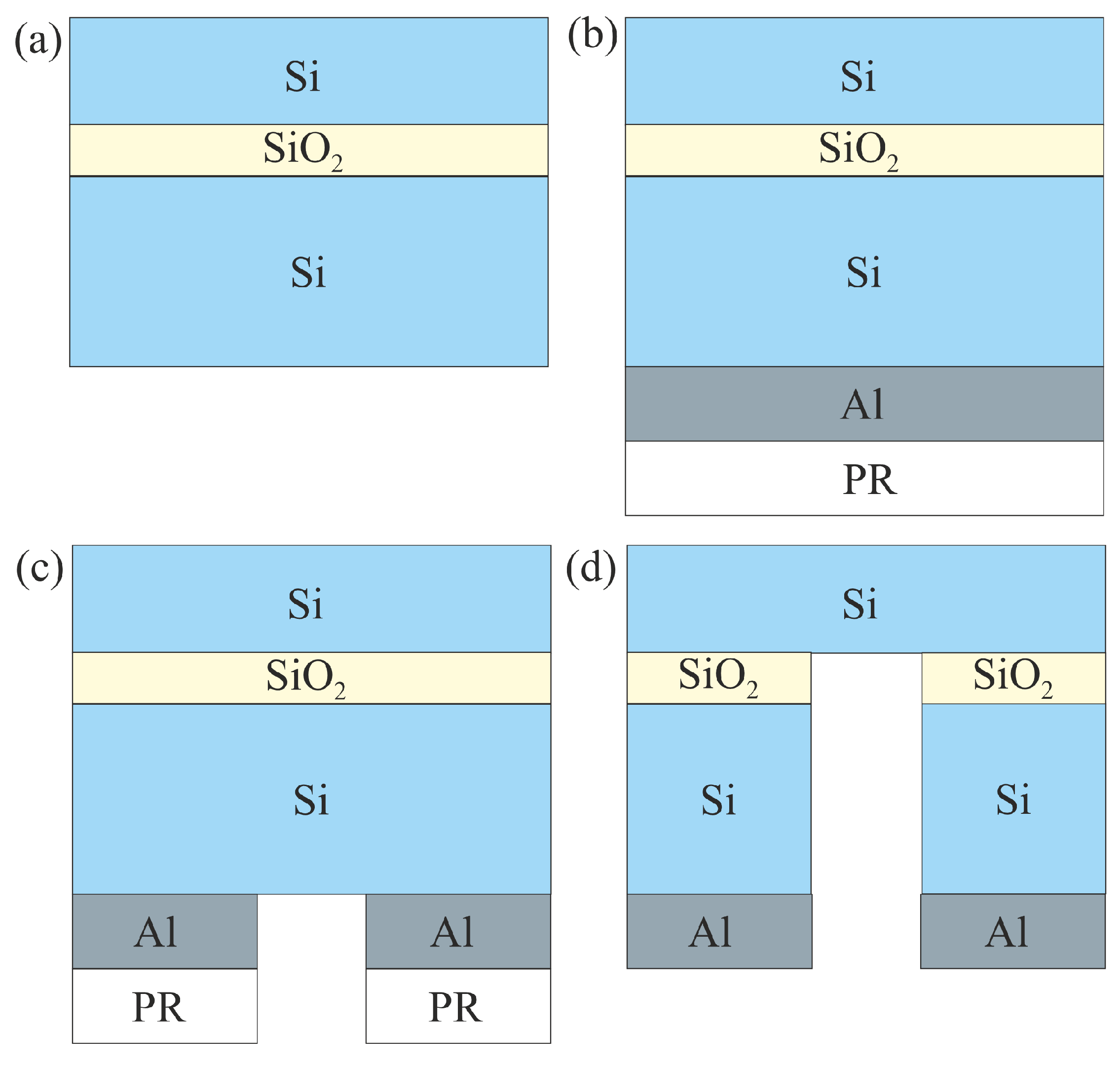
Figure 2.
Experimental setup for measuring the mechanical properties of thin-film membrane structures at non-zero pressure: gas pipe line (1), filter regulator MC104- D00 (2), pressure regulator ER104-5PAP (3), personal computer (4), profilometer Veeco Wyko NT9300 (5). The inset on the right: an image of a crystal with SOI-based single-crystal Si membrane fixed in the holder of the open part of the pipe line when applying zero and non-zero air pressure, respectively
Figure 2.
Experimental setup for measuring the mechanical properties of thin-film membrane structures at non-zero pressure: gas pipe line (1), filter regulator MC104- D00 (2), pressure regulator ER104-5PAP (3), personal computer (4), profilometer Veeco Wyko NT9300 (5). The inset on the right: an image of a crystal with SOI-based single-crystal Si membrane fixed in the holder of the open part of the pipe line when applying zero and non-zero air pressure, respectively
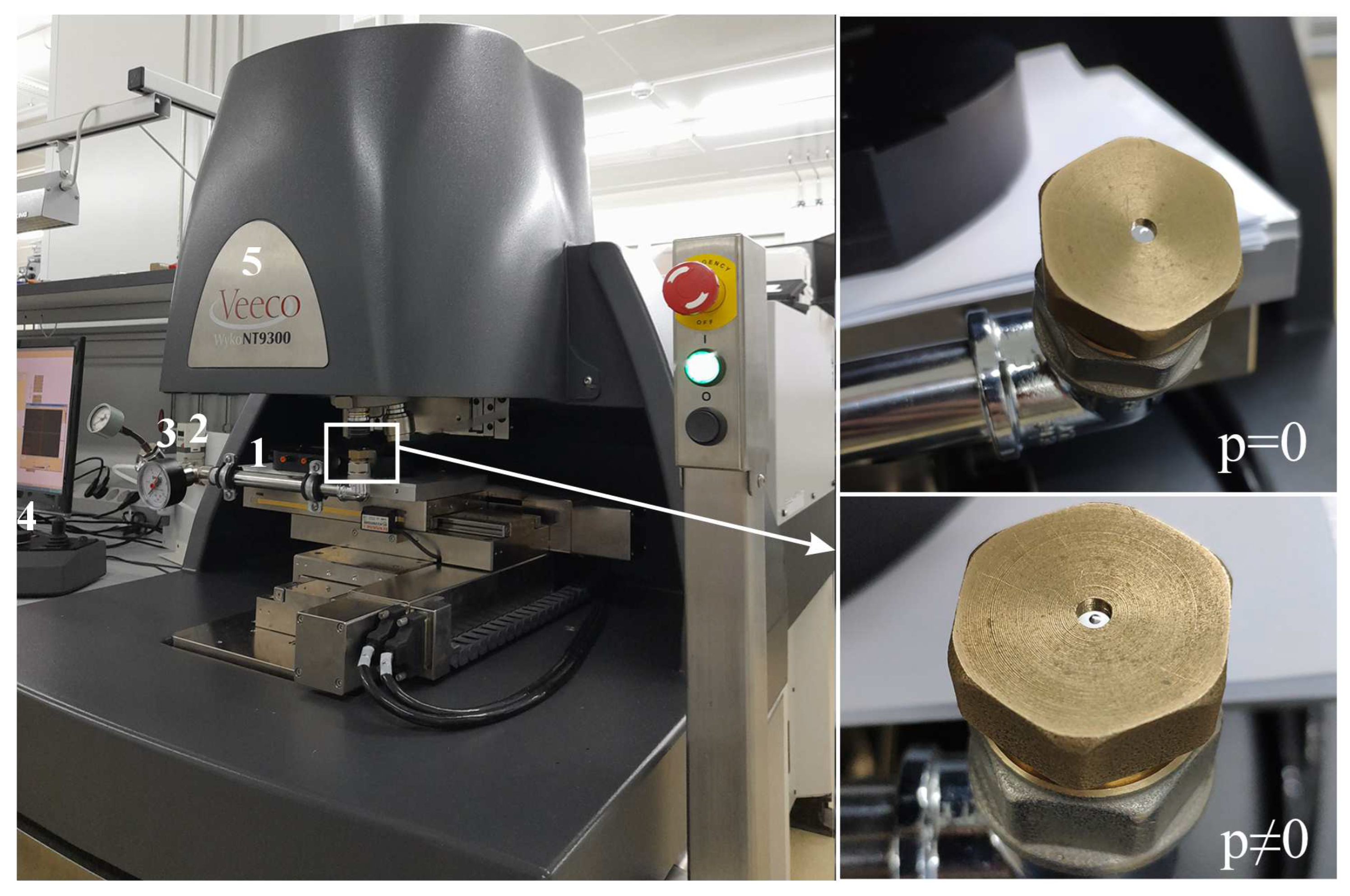
Figure 3.
Schematic of the experimental setup. Gas (air) is supplied through a pipe line to the sample, where the gas pressure is automatically adjusted through the Arduino Mega 2560 board (which is connected to PC1), while the profile of the structure is taken by a Veeco Wyko NT9300 profilometer and then sent to PC2.
Figure 3.
Schematic of the experimental setup. Gas (air) is supplied through a pipe line to the sample, where the gas pressure is automatically adjusted through the Arduino Mega 2560 board (which is connected to PC1), while the profile of the structure is taken by a Veeco Wyko NT9300 profilometer and then sent to PC2.

Figure 4.
Measured vertical coordinate of the profile of the fabricated single-crystal Si membrane under the different applied pressure p: (a) measurement #1 for test sample 1, (b) measurement #2 for test sample 2.
Figure 4.
Measured vertical coordinate of the profile of the fabricated single-crystal Si membrane under the different applied pressure p: (a) measurement #1 for test sample 1, (b) measurement #2 for test sample 2.
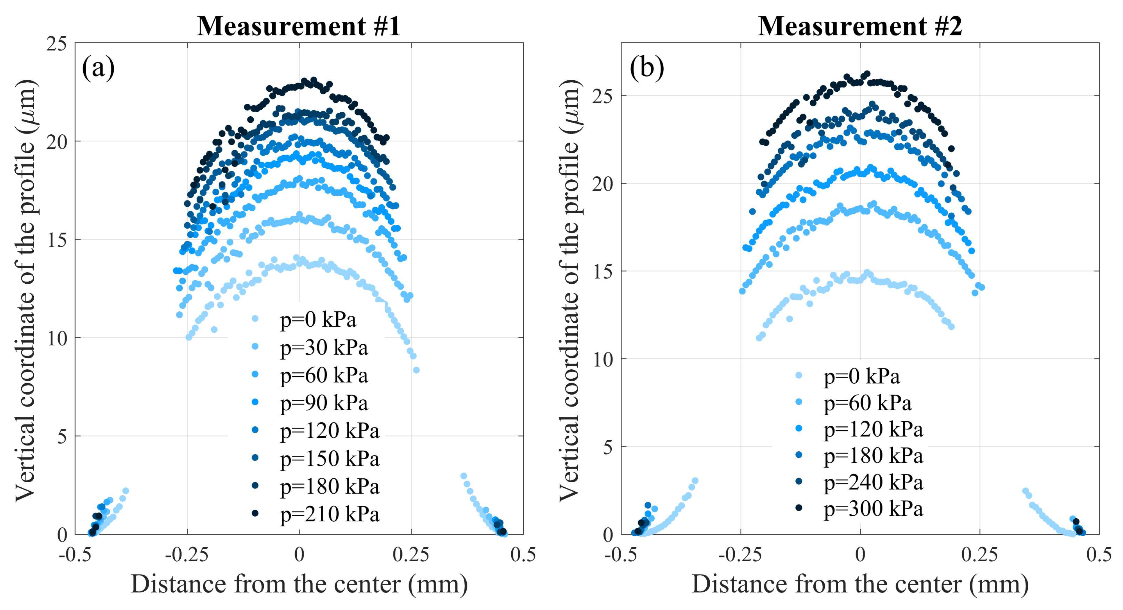
Figure 5.
Design diagram of the plate
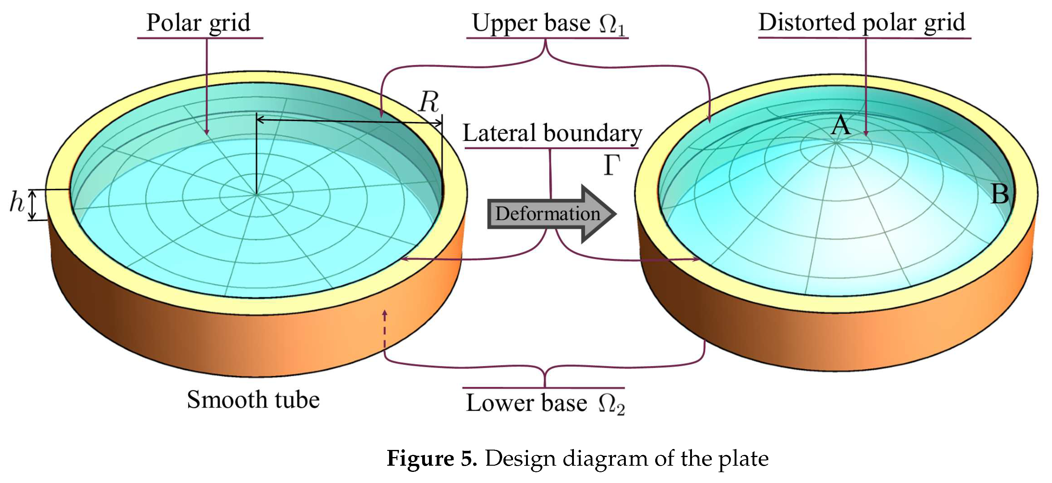
Figure 6.
Comparison of displacement fields for different values of the anisotropy factor
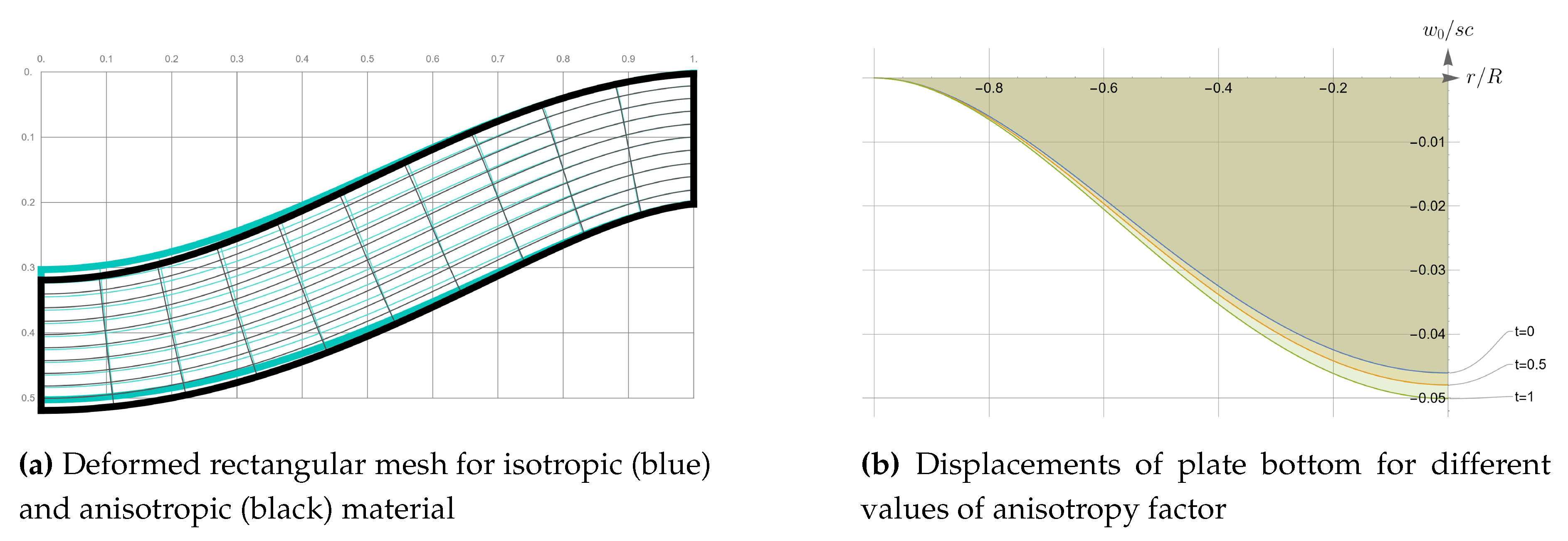
Figure 7.
Pressure-displacement curve
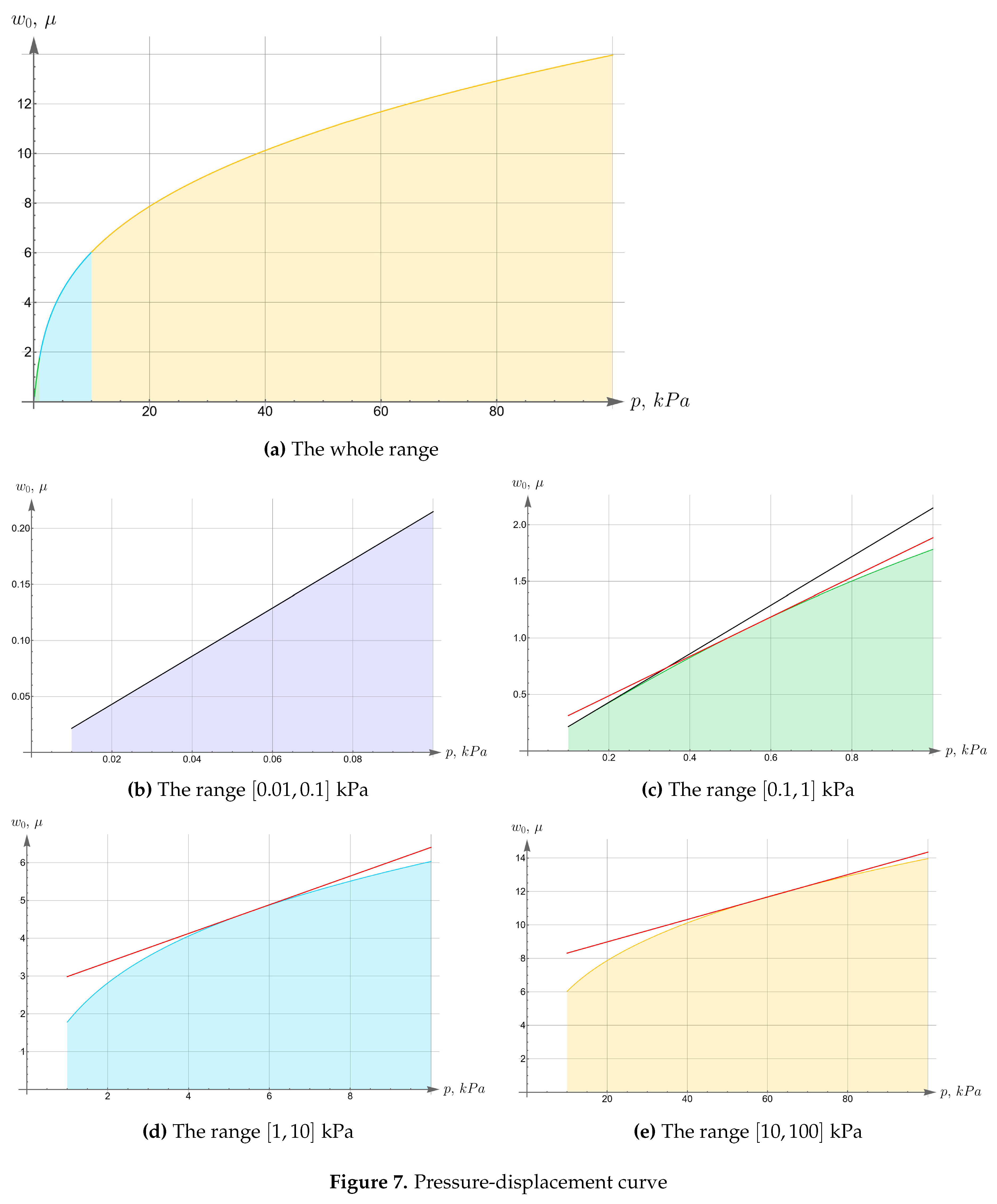
Figure 8.
Displacements of the bottom surface for different values of the initial in-plane tension
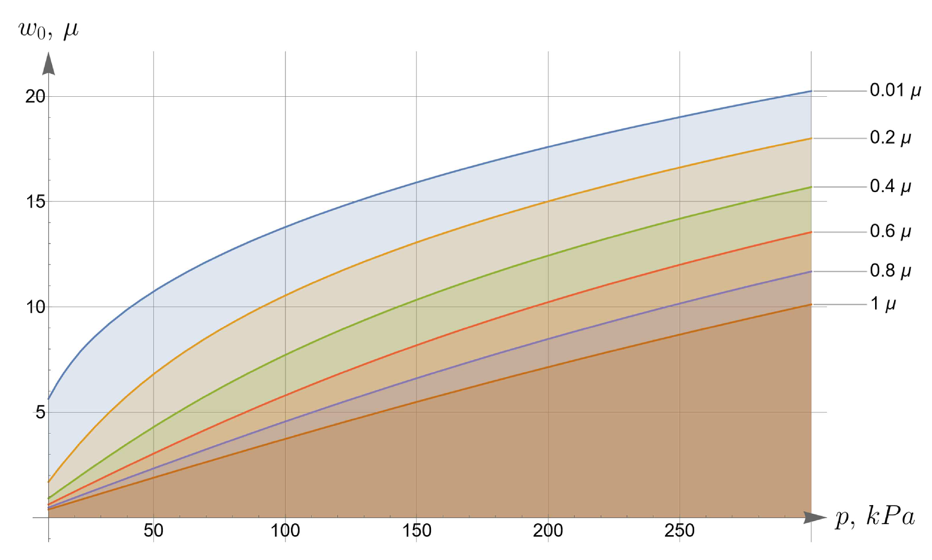
Figure 9.
Experimental data in first series
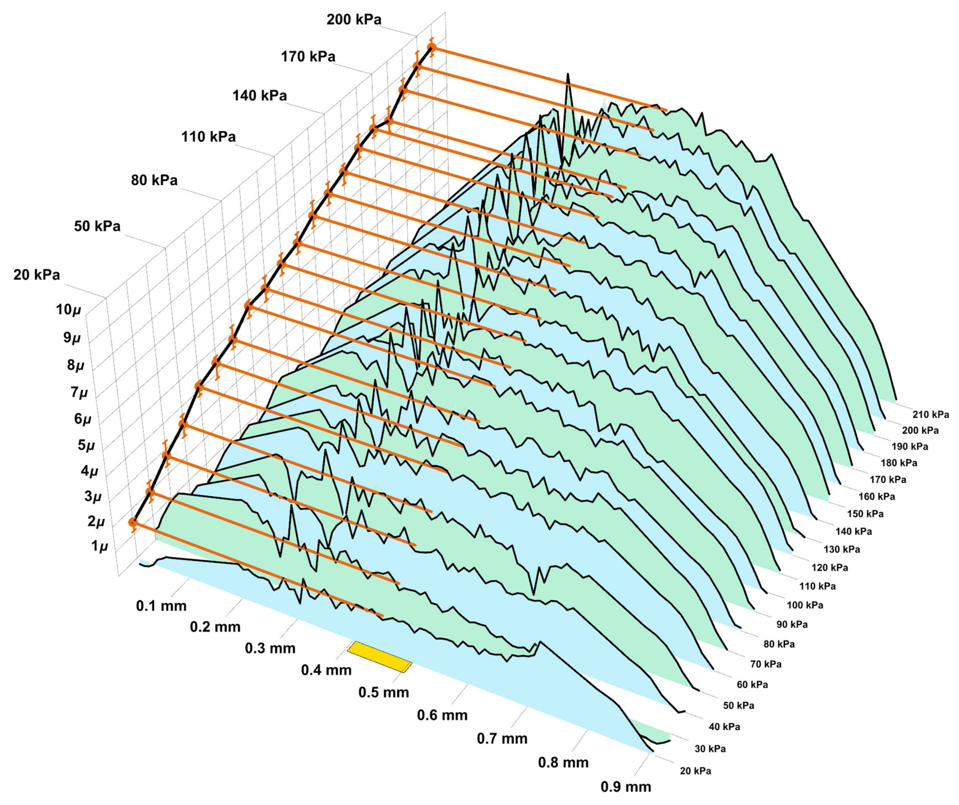
Figure 10.
Experimental data in second series
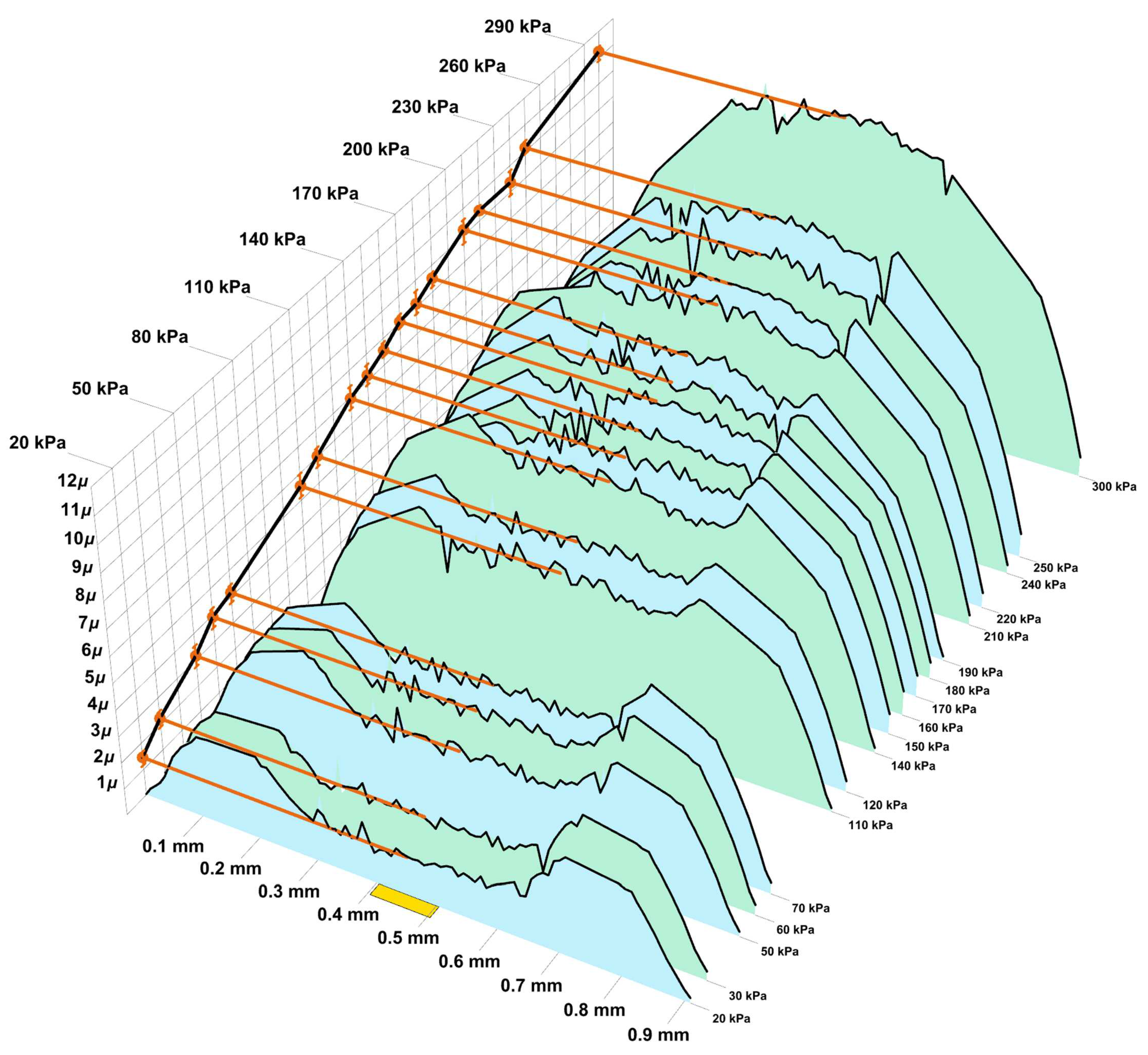
Figure 11.
On the issue of identifying the initial tension
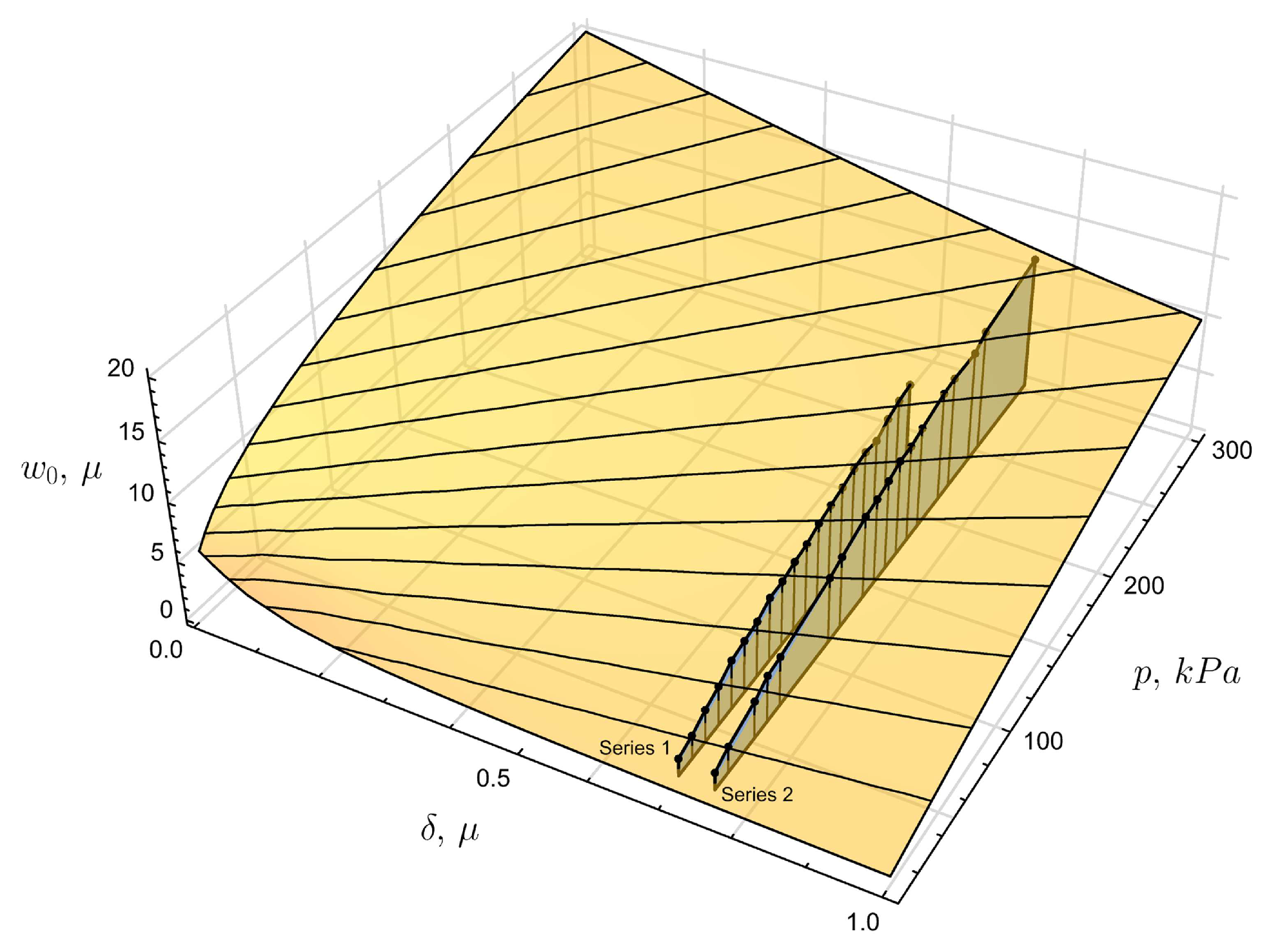
Figure 12.
Comparison of theoretical and experimental displacements
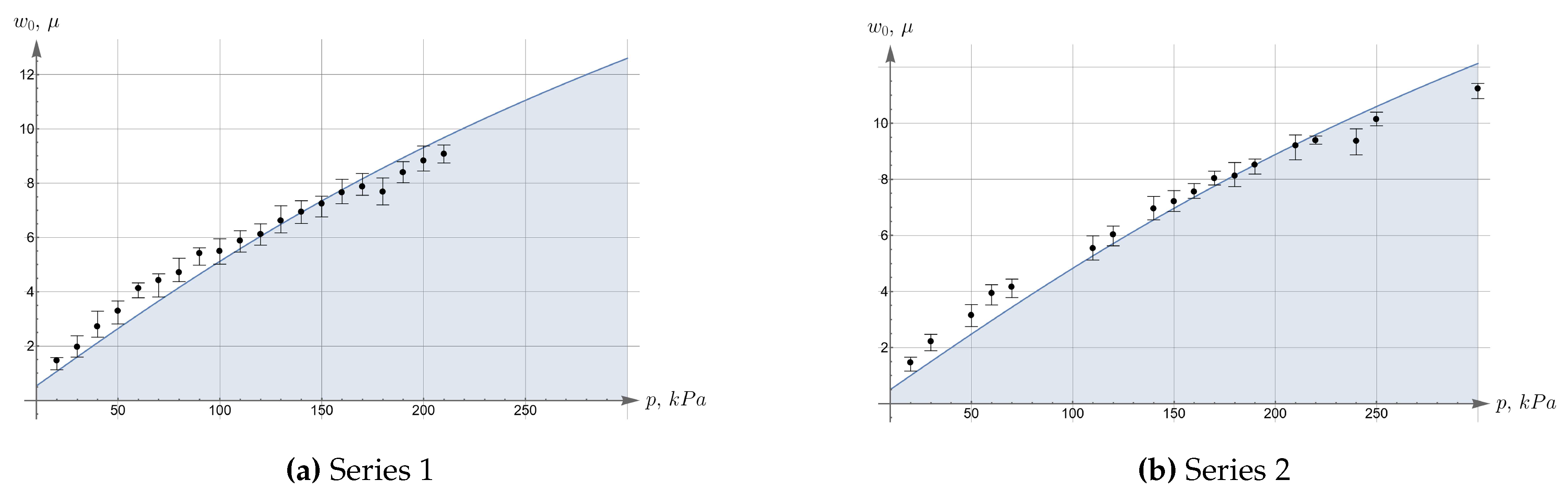
Table 2.
Dimensionless components of stresses with respect to anisotropic factor
| Point A | Point B | Point C | |||||||
|---|---|---|---|---|---|---|---|---|---|
| t | 0 | 0.5 | 1 | 0 | 0.5 | 1 | 0 | 0.5 | 1 |
| 0.1236 | 0.1248 | 0.1261 | 0 | 0 | 0 | 0.1969 | 0.1969 | 0.1969 | |
| 0 | 0 | 0 | 6.136E-4 | 6.1364E-4 | 6.1364E-4 | 0 | 0 | 0 | |
| 0.1236 | 0.1248 | 0.1261 | 0 | 0 | 0 | 0.04554 | 0.04792 | 0.05040 | |
Table 3.
Slope of tangents in different intervals of pressure-displacement curve
| Interval | ||||
|---|---|---|---|---|
| Slope |
Table 4.
Approximate formulae for plate deflections
| Kirchhoff – Love theory | |
|---|---|
| Föppl – von Kármán theory | |
| Empirical formula |
Table 5.
The difference between the proposed solution and the approximations used in structural mechanics
Table 5.
The difference between the proposed solution and the approximations used in structural mechanics
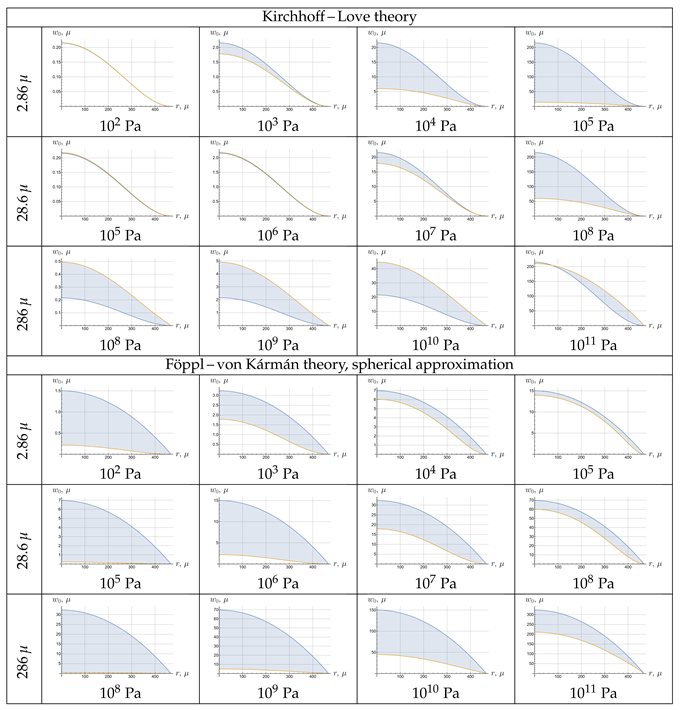 |
Table 6.
The difference between experimental and theoretical deflections
| Series1 | 7.2417 | 0.6978 | 7.3461 (1.4%) | 17.1867 (137%) | 7.9039 (9.1%) |
| Series2 | 7.2079 | 0.7484 | 6.9659 (3.4%) | 17.1867 (138%) | 7.4864 (3.9%) |
Disclaimer/Publisher’s Note: The statements, opinions and data contained in all publications are solely those of the individual author(s) and contributor(s) and not of MDPI and/or the editor(s). MDPI and/or the editor(s) disclaim responsibility for any injury to people or property resulting from any ideas, methods, instructions or products referred to in the content. |
© 2023 by the authors. Licensee MDPI, Basel, Switzerland. This article is an open access article distributed under the terms and conditions of the Creative Commons Attribution (CC BY) license (http://creativecommons.org/licenses/by/4.0/).
Copyright: This open access article is published under a Creative Commons CC BY 4.0 license, which permit the free download, distribution, and reuse, provided that the author and preprint are cited in any reuse.


