Submitted:
24 November 2024
Posted:
26 November 2024
You are already at the latest version
Abstract
The solution of non-linear system of the Foppl -- von Kármán equations for squared plates is obtained in the form of decomposition over a basis in the space of square-integrable functions. To define such a basis a system of eigenfunctions of a linear self-adjoint operator is used. The coefficients of expansion are determined via reduction method from the infinite-dimensional system of cubic equations. This allows the proposed solution to be considered as a non-linear generalization of classical Galerkin approach. The novelty of the study is in the strict formulation of the auxiliary boundary problem, which makes it possible to take into account complete plate fixation along the boundary. To verify proposed solution it is compared with experimental data. The latter is obtained by holographic interferometry of small deflection increments superimposed on the large deflection caused by initial pressure. Experiment and theory showed good agreement.
Keywords:
Foppl -- von Kármán equations
; Finite deformations
; Clamped square plates
; Non-linear PDEs
; Expansion over a basis in space of square-integrable functions
; Galerkin method
; Infinite-dimensional system of cubic equations
; Reduction
; Experimental verification
1. Introduction
The Föppl – von Kármán equations, which describe stress-strain state of flexible plates, has attracted attention of physicists and mathematicians since August Föppl introduced their prototype in the treatise "Vorlesungen uber technische Mechanik" [1]. A. Föppl assumed that in the case of finite deflections, both in-plane linear strains and the rotations are small with respect to unity, while the rotations and squares of in-plane strains are infinitesimals of the same order. Furthermore, he supposed that the bending strains can be thought of infinitesimally small with respect to membrane ones. With these assumptions he derived the following system of equations:
Here is a plate thickness, denotes Young’s modulus of its material and is the function of transversal load applied to the plate surface. The function represents the deflections of the plate middle-plane, while is the Airy stress function related with the components of the stress tensor within it:
Symbols and stand for the biharmonic operator and the Monge – Ampère form [2], respectively. In Cartesian coordinates they can be represent as follows:
Theodor von Kármán improved first equation in (1) by adding an item that accounts for influence of in-plane stresses on bending and derived the system of equations in a well-known almost symmetric form [3]:
Here denotes the bending stiffness of the plate, which expressed through and the Poisson’s ratio : .
The Föppl – von Kármán equations were initially developed as a mathematical tool for buckling analyses of ship hall parts [4]. However, wide application of the structural elements that were able to bend sufficiently without undergoing plastic deformations calls for further development and improvement of the non-linear theories of plates, subjected to various loads, including transverse one. The Föppl – von Kármán equations proved to be a good approach, taking into account non-linear effects but not having the intimidating bulky form of the non-linear elasticity equations. At present in many modern technologies, particularly MEMS, the problem of mathematical modelling of stress-strain state in flexible parts is extremely relevant [5,6].
First solutions of non-linear bending problem were obtained for circular plates subjected to axial symmetric loading, which allowed one to significantly simplify the Föppl – von Kármán equations. Thus, the first attempt to solve them for a clamped circular plate under uniform pressure was undertaken by Nádai [7] in 1925. Another variants of approximate solution were obtained by Timoshenko who used the Rayleigh – Ritz method [8] and by Way through the power series expansions [9]. In the first part of their study [10], Friedrichs and Stoker presented numerical solutions for a simply supported circular plate under compressive forces at the boundary, obtained by three distinct algorithms. Furthermore, in [11] they introduced a change of variables, which reduced the order of the governing system of equations from 8th to 4th. In addition, in the second part of [10], they presented a proof of the existence theorem and demonstrated that, apart from a trivial solution, there is at most another one (accurate to a sign). In present paper, only square plates will be discussed, so the part of review focused on circular plates is exhausted by a few references. A detailed survey can be found in [12].
One of the first approximate solutions of the Föppl – von Kármán equations for a simply supported square plate under uniformly pressure was derived by Kaiser [13] using finite-differences method. An alternative approach to approximate solution was proposed by Way [14]. He obtained solution for clamped rectangular plates with various aspect ratios by Ritz method. The Galerkin method was also successfully applied for this problem by Panov [15]. Levy first derived exact solutions in terms of double Fourier series for a simply supported rectangular plate [16] and a clamped square one [17]. Later, he and Greenman solved the problem for a clamped rectangular plate having an aspect ratio of 3/2 [18]. This method also has been applied in [19] and [20] for long clamped and simply supported plates under combined load. It is important to note that in works [16,17,18,19] it is assumed that clamped edges are movable they are rigidly clamped against normal displacements and rotations while allowing for movement in plane. A numerical solution for a clamped rectangular plate with immovable edges was obtained by Wang [21]. He also considered the important case of a riveted panel [22]. Lastly, it is worthy noting the article by Green and Southwell on the application of the relaxation method to solve the Föppl – von Kármán system [23]. A detailed description of the majority of the aforementioned results, as well as many others, can be found in the remarkable books [4,24].
Briefly discuss the recent work on this topic. In the works [25,26] the solution for a simply supported plate was obtained by the "accelerated" iterative method. The perturbation method was successfully applied in the works [27,28,29,30]. In addition, the work [29] is notable because of application of the spline function method for solving a set of linear equations. A number of authors successfully applied the finite-difference method [31,32,33]. A modification of this approach was proposed by Petit [34], who employed the finite-difference method in combination with the relaxation one. Furthermore this method was also used in the work [35] for a plate under combined load. The finite elements method was widely used [36,37,38,39]. Also, a few attempts to apply the boundary elements method were made [40,41,42,43,44]. The Ritz method was widely used as well. Boresi and Terner [45] applied it to obtain the solution for a simply supported rectangular plate with stress-free edges. In the work [46] the rectangular plates with various boundary conditions were considered using the automated Ritz method procedure. This procedure was also applied to calculate large deflections of orthotropic plates [47] and functionally graded material ones [48]. Enem [49] introduced the Ritz method solutions for rectangular plates with twelve different boundary conditions. Recently, the homotopy analysis method has begun to be successfully applied to solve the Föppl – von Kármán system [50,51,52,53]. A sufficiently detailed review of works managed before the 1970s are presented in the article [54]. Also, a comprehensive list of works managed before the 2000s is given in the book [55], while detailed review containing more recent works can be found, for example, in the PhD thesis by Khoa [56].
An original approach to solve the Föppl – von Kármán system was proposed by H. Berger in his PhD thesis [57]. This approach was based on the hypothesis that the strain tensor second invariant makes a small contribution to the full potential energy in comparison with the contribution made by the first invariant. Although this hypothesis lacked a physical basis, it allowed one to decouple the Föppl – von Kármán system. Berger obtained solutions for circular and rectangular plates with various boundary conditions using this method. The further development of Berger’s technique was continued by a number of other scientists [58,59,60,61]. A similar method for decoupling the Föppl – von Kármán equations was employed in the recent works [62,63,64]. An alternative approach to decoupling of this system system was proposed by Banerjee and Datta [65].
A large amount of results were obtained by the Galerkin method. Yamaki [66] used a modification of the one-term Galerkin method to solve the dynamic analogue of the Föppl – von Kármán equations. He also gave a classification of flexible plate boundary conditions. In their work [67], Iyengar and Naqvi applied biorthogonal expansions of the displacements and the Airy function to obtain a solutions for a simply supported plate and a clamped one. For each boundary condition type two options were considered: all edges are stress-free and all edges are immovable. In the papers [68,69] the authors obtained the Galerkin method based system of cubic equations for Kármán plates in an explicit form. In the work [70] this result was supplemented with the explicit expression of the inverted Galerkin matrix. This procedure allowed to obtain the solution more effectively due to avoiding a laborious calculation of the inverted Galerkin matrix. Recently, the wavelet-Galerkin method has been widely used [71,72]. This method leads to simplification of calculations due to the choice of wavelet functions as the basis.
It is advisable to consider some works devoted to analyse of the Föppl – von Kármán equations in term of pure maths. Initially, they did not have a rigorous mathematical justification and were derived through an engineering approach significantly based on a few auxiliary hypotheses [2]. The justification of this system has been provided by Ciarlet, who has demonstrated [2,73] that this system can be obtained using the asymptotic expansion of the equations of non-linear elasticity theory by a small parameter, assuming certain hypotheses about the asymptotic orders of displacement vector components. This approach was also applied in the recent work [74] to construct the family of Kármán-like plate models.
The existence theorem for the Föppl – von Kármán boundary-value problem with sufficiently smooth boundary and homogeneous boundary conditions was proofed by Morozov [75] using the Leray –- Schauder method [76]. The conditions for the existence of a non-trivial equilibrium state of a Kármán plate under compression forces were formulated by M. Berger and Fife [77]. Knightly [78] demonstrated the existence of a solution for a plate subjected to combined loading, and moreover, he proofed that if the magnitude of the loading is sufficiently small, then this problem has a unique solution. Further, Knightly and Sather [79] have modified this uniqueness result. Hlaváček and Naumann have obtained similar results for the various types of inhomogeneous boundary conditions [80,81]. It is important to highlight that results of Knightly, Hlaváček and Naumann are applicable to plates with the boundary which consists of curves from and may have corners at junctions of the arcs they are valid for the majority of plates used in engineering.
From this brief analysis, it is observed that, to date there is no long-standing methods to solve Föppl – von Kármán equations for square and rectangular plates fixed at the boundary with respect to all displacement components. Moreover, direct 3D FEM modelling of thin plates results in a ill-conditioned algebraic system due to the small parameter, which is the plate thickness. However, it is the full fixation that is usually implemented in experiment and practice. In this context, the development of Föppl – von Kármán equations solution methods for square and rectangular plates, fully fixed at the boundary, is an urgent problem in computational mechanics. This is the subject of present paper. In it a new solution is proposed in the form of decomposition over basis in functional space of square-integrable functions. The coefficients of expansion are determined from infinite-dimensional cubic system via reduction method. This approach could provide a non-linear counterpart to Galerkin method. The principle difference from similar studies [67,70] consist in a strict formulation of the auxiliary boundary problem, allowing for account natural ways of plate fixing.
2. Problem Statement
Consider a clamped square plate of side 2 and thickness , made from a linear-elastic material with moduli , and subjected to an arbitrary transversal load (see Figure 1). For a closed formulation of the initial boundary problem, we should complement the equations (4) with suitable boundary conditions, which we will now deal with. The boundary value problem will be formulated in the region: ,
with the boundary: ,
where the parts of the boundary correspond to pairs of opposite edges,
The boundary conditions for the flexible plates usually are gathered into two sequences associated with plate bending and with plane stress-strain state respectively. Consider the first one. In the case of clamped plates it can be written as: .
Other variants of the boundary conditions related to bending are well known [24], and we will not comment on them as (5) are the ones that will be stated hereinafter. The boundary conditions associated with in-plain stress-strain state are not so widely covered in literature and we will discuss their formulation in more detail. Following [17,21] we consider two cases:
– movable edges: ;
– immovable edges: .
Note that despite the designation, moving edges are not free from fixing at all. The points on them can only be moved along the edges, while their displacement in a perpendicular direction is constrained. In equations (6a), (6b) and denote the in-plane plate displacements (the in-plane displacements of the points on the plate middle plane). These functions are not explicitly included in the governing system (4), so in order to resolve the boundary-value problem, it is necessary to express them through the desired functions . The sought relations can be obtained using the Cesàro formula, which express the displacement vector and the rotation vector via the infinitesimal strain tensor [82]: .
Note that the displacement vector is defined with account of kinematic hypothesis of the Kirchhoff-like plate theory: .
Therefore, to relate the displacements to the Airy stress function , it is necessary to express the infinitesimal strain tensor through the stress tensor . The essence of Kármán theory based on a number of simplifications which allow only the use Saint Venant – Kirchhoff constitutive equation [73,83]: ,
where is the reduced Green – Saint Venant strain tensor (also known as the Kármán strains): .
Finally, substituting the relation (9) into the Cesàro formula (7) one can obtain:
This formula can be significantly simplified by choosing an appropriate path of integration. Taking into account that displacements and rotations of whole plate are defined up to an additive constants, any point of it can be fixed. Apart from that, if the transversal load function is odd or even by both coordinates then the centre of a plate will be displaced vertically without changing its in-plane position. For the sake of simplicity, assume that the load function and, as a consequence, sought functions are even by both coordinates (three other cases of symmetry are derived from reasoning completely similar to the following): .
Here we also restrict the class of considered functions only by square-integrable ones. This allows to decompose them over basis and reduce the boundary-value problem to a system of cubic equations.
With account of the transversal loading function symmetry (10) the displacement on can be calculated as follows:
Substitution of equations (8) and the relations (2) into above formulae results in:
However, taking into account that a function is identically zero iff it takes value zero at least at one point and its the first derivative is zero also, the latter integral condition can be reduced to a differential relation:
The last terms in the right-hand sides of this relation can be omitted due to the fact that the deflection function is identically zero on the edges (5):
Thus, above relation together with the first integral equality (5) fully describes the boundary conditions for the in-plane displacements of the plate on . The formulae for the boundary conditions on can be written in the similar way up to replacement of the variable by and function by respectively.
Now we can move on to formulation of boundary value problem. To this end introduce the following dimensionless variables: .
In the new variables the Föppl – von Kármán equations (4) and corresponding boundary conditions can be written as:
– movable edges: ;
– immovable edges:
where , . In the what follows, we will omit the tildes above these operators for brevity. The equations (6) – (13) or (9) constitute two different boundary-value problems for clamped square plate.
To obtain an approximate solution of the problem (6) – (13) or (9) a recursive approach is often used. Briefly describe its essence for comparison with the proposed solution below. The basis of the recursion can be taken as a solution of the Sophie Germain – Lagrange equation:
while the step of the recursion is defined as follows (here subscript indicates recursion step number):
Stress function can be obtained on each step from the relation
Here stand for differential operators, defined by the same biharmonic differential expression (3).1, but by different boundary conditions, corresponding to deflection () and stress function (), (13), (9). Computational efficiency of recursive process depends on way how to represent inverse linear operators and . It can be done differently, but for square plates the usage of complex potentials method (Goursat – Muskhelishvili – Kalandiya) [84] seems to be most appropriate. Within this method one can define the solution of linear problem as the sum of some particular solution that satisfy non-homogeneous biharmonic differential equation, but not met boundary conditions, and boundary solution of homogeneous equation , such that satisfies the conditions on the boundary.
Particular solution can be obtained as
or
while the boundary solution can be expressed in terms of complex-valued series with respect to as follows:
Here:
where can be obtained from the solution of algebraic counterpart for boundary problem (see [84,85] for details). In above formulae indicates the complex conjugate z while stands for conformal map between unit disk and rectangular domain. This mapping can be exactly expressed via hypergeometric function, but for computations it is more continent to use polynomial approximation of order n:
The inverse operator can be obtained in a similar way. Note, that the advantage of complex potential method is that the integral boundary conditions can be expressed directly via potentials with Love relations:
Before embarking on general procedure of problem (6) – (13), (9) solution let us try to approach it with recursive method mentioned above. In doing so, keep in mind that in order to identify the characteristic features of non-linear deformation of the plate, it is sufficient to perform at least one step of recursion. The calculation results for the model problem are shown in Figure 2. In it the subfigure (a) shows the distribution of deflections obtained without of account non-linear effects (it is the base or recursion, solution of the Sophie Germain – Lagrange problem). Subfigure (b) shows the distribution of plain deformation incompatibility, induced by bending, namely . In subfigure (c) one can see stress function , corresponding to such incompatibility. In the second line of figures the distributions for normal and tangential in-plane stresses are shown, while the last subfigure (f) demonstrates dummy transverse loading that has to be subtracted from actual loading on the first recursive step.
Already from the analysis of the results obtained in the first step of recursion, it is possible to give a qualitative estimate of the effect of the dummy load and, accordingly, of the non-linear effects depending on the expected value of the maximum deflections. In particular, with evenly distributed load the maximal value of dummy load (according to the distribution, shown in Figure 9.(f) for some load with dimensionless intensity can be estimated as . Therefore, the given and dummy loads will be of the same order when , that, with account of distribution for deflections (Figure 9.a), is approximately equivalent to maximum deflections, obtained in linear approach, of 20% from the edge length of the plate. This value is a very rough estimate from above, because in fact the displacements will be much lower if we take into account non-linear effects, calculating the following recursion steps. Also, it can be noticed that:
– the influence of the dummy load increases proportionally to the cube of maximum deflection;
– the geometric shape of the bending surface at the final deformation significantly differs from the corresponding shape for small deflections, because the dummy load changes the distribution of RHS of bending equation on successive recurrent steps. We will see this again later when we consider the general procedure of solution.
Mentioned above strategy for solution of non-linear bending problem has computational stability for moderate bending only. When the amount of deflection increases, the dummy load is no longer a small adjustment and may even exceed given transverse load. In this case the sequence of recursively constructed approximations tends to diverge. Although special regularization procedures [5] can be used, diverging cannot be avoided. For this reason, below a different strategy is proposed, implementing the full algebraization of the problem and transforming it to the infinite-dimensional system of cubic equations. Reducing this system to a finite-dimensional one and using any variation of the successive approximation method to find the solution of the reduced system, it is possible to avoid computational instability even for deflections that are comparable with the size of the plate in the plane. The rest of the article is devoted to the construction and analysis of such algebraization.
3. Solution of the Linear Problem
Since the solution of the non-linear problem will be obtained in the form of decomposition over some basis in , generated by a linear self-adjoined operator, we will start with the linear problem. It is advisable to consider the linear bending of a square plate as such prototype for this problem, because, first, it generates a basis in terms of well-known Krylov-Duncan functions, and second, the problem itself can be used for testing a non-linear solution at zero approach.
The boundary-value problem for clamped Sophie Germain’s plate can be stated as follows:
In order to expand the deflection function into a Fourier series, it is necessary to choose a basis in . According to the Hilbert – Schmidt theorem [86], a system of eigenfunctions of any compact self-adjoint operator constitutes a basis of . However, the biharmonic operator has sufficiently complicated system of eigenfunctions even with homogeneous boundary conditions, so it is more preferable to use an another self-adjoint operator. It is appropriate to use the operator constructed by removing a mixed derivative from the biharmonic one: .
The sequence of eigenfunctions for this operator can be obtained as a combination of solutions of an auxiliary Sturm – Liouville problem.
3.1. Auxiliary Sturm – Liouville Problem
Let us consider a Sturm – Liouville problem:
A fundamental system of solutions for this equation is well-known: .
By substituting a linear combination of these functions into the boundary conditions, we get the spectral equation with respect to eigenvalues : .
Thus, a spectrum of the operator consists from two sequences of eigenvalues 1:
which are defined as roots of transcendental equations:
These roots can be found numerically with arbitrary precision, but for sufficiently large values of very precise approximations can be obtained from asymptotic formulae:
The question arises: what does it mean to be large enough? The following computation (Table 1 and Table 2) shows that for standard machine precision it enough to refine only five first values, while all the rest can be calculated directly by the formulae (11). Of course, for calculations with enhanced accuracy the number of refined roots should be increased.
Each sequence of the eigenvalues is associated with a sequence of the auxiliary eigenfunctions:
Such sequences of function are convenient for derivations because their compact view, however for calculations it is more convenient to use normalized functions:
Curves of the first several normalized eigenfunctions are shown in Figure 3.
It is evident that each pairwise combination of functions (12) presents a eigenfunction of two-dimensional operator . Thus, we arrive at four families of eigenfunctions for : .
Although each term of these families is marked by two indexes, it is preferable to use a one-indexed numeration system. Such system can be provided by any bijection . The optimal numeration system is well-known from classical courses of calculus: .
This bijection is named the Cantor pairing function for the positive integers and was proposed by him in the article [87]. The correspondence between two systems of numeration can be illustrated by a diagram as shown in Figure 3 (c). This way for numeration is the most preferable for square regions because it allows one to construct the reduced sums symmetric with respect to both indices. In order to achieve this, it is sufficient to include complete diagonals in the sum.
Thus the two-indexed system of basis functions (29) can be replaced by the following one: .
One can go back to the functions (29) with reverse function to (30). In order to construct this function it is necessary to relate a number of the current term with the number of diagonal on which this term is located: ,
where the symbols denotes the floor. From here, it is simple to obtain the inverse function: .
Hereinafter and are brief notations for components of the inverse function.
3.2. Solution of the Linear Boundary-Value Problem
Now it is time to recover the boundary-value problem (), (10). We will seek the solution of this problem in the form of expansion in terms of a series of normalized basis functions (35): .
This solution is guaranteed to satisfy the boundary conditions () due to the appropriate choice of the basis. Consequently, in order to solve the boundary-value problem, it is sufficient to find the Fourier coefficients , with which (37) satisfy inhomogeneous Sophie Germain – Lagrange equation (10).1: .
Here with we denote the eigenvalues of the operator :
One can find by acting the projection operators: ,
on both sides of equation (38):
It is essential to note that the basis functions lying in different sequences have a different parity. Consequently, due to the fact that the second derivative of any function has the same parity as the function itself, the double sum in the previous relation can be reduced to the sum:
Thus, the differential equation is reduced to an infinite-dimensional system of algebraic equations. By applying the reduction method [88,89] we arrive at the sequence of finite-dimensional systems of linear algebraic equations which can be written in a matrix form: ,
where are matrices × known as Galerkin matrices. Their components, can be obtained via formula 2: .
Vector contains Fourier coefficients of transverse load function (for brevity, we will refer on it as load vector): .
Recall now that we consider functions only from (10), so it is sufficient to calculate only the first Galerkin matrix and the first load vector , which correspond to even by both variables functions. In this regard hereinafter we will omit the first index and adopt the following notations:
Thus, the problem has been reduced to one matrix equation. In the case of an arbitrary non-symmetric load function, further steps would be similar, however they will require finding of all matrices and vectors .
Proceed now to calculating of Galerkin matrix and load vector components. It is convenient to represent an expression for them using an auxiliary integral 3:
where denote norms of the basis functions: .
The components of the load vector are calculated by formula (42) is assume .
Now the Fourier coefficients can be calculated from the first matrix equation system (40) using, for example, Cramer’s rule: .
Here is the identity matrix and are so-called matrix units which have only one unit component with indexes , while other components are zero.
Finally, the solution can be obtained by summing the basis functions with the calculated Fourier coefficients : .
The above limit exists because the original infinite system is fully regular (see [89]). It should be noted that the formulae (47), based on Cramer’s rule, are merely of academic interest, while in numerical realization it is convenient to use more efficient algorithms of matrix inverting.
To illustrate obtained solution model calculations were performed for two type of load function: uniform load, and bump-function, which is defined within the region as polynomial function and is zero outside of it. Trial load function and their approximations by reduced Fourier sums are shown in Figure 4. The purpose of these calculations is to show how the convergence rate of the sequence of partial sums depends on the smoothness of the load function and its belonging to the differential operator’s domain (obviously the first function does not belong to the domain, whereas the second one belongs to it).
Results of these calculations are presented in Figure 5 and Figure 6. Subfigures (a) contain deflected shapes of plate. In subfigures (b) the inaccuracy functions for corresponding load functions are shown, which is defined as distributions of unbalanced transversal forces absolute values:
Subfigures (c) give integral estimations of the inaccuracy functions versus number of accounted terms in reduced sums:
In these subfigures, the orange points correspond to sums that are symmetric with respect to the coordinates with any term they contain a symmetric term .
4. Solution of the Föppl-von Kármán System
Proceed to solving the Föppl-von Kármán boundary-value problems (6) – (13) and (6) – (9). As above we will represent the unknown functions and as decompositions over basis functions (35). However, in this case such expansions do not allow the boundary conditions to be satisfied automatically. In order to overcome this difficulty, we augment the decompositions by the solution of the specific boundary problem.
4.1. Auxiliary Boundary Problem
Consider a homogenous biharmonic equation with the following boundary conditions:
where are arbitrary square-integrable functions. The solution of this problem can be found in the form of a sum: ,
where meets inhomogeneous boundary conditions () but not satisfy homogeneous biharmonic equation (). Another summand , instead, meets homogeneous boundary condition and inhomogeneous equation:
Thus, the sum (63) will represent the solution of the boundary problem (), ().
Taking into account symmetry relation (10) it is possible to simplify boundary conditions ():
where is an even function, while is an odd one. In this case, the function may be presented as follows:
Substitution of this function in () results in expansions of functions and into the Fourier series:
Thus, this solution allows one to satisfy any boundary conditions that may occur in the case of the loading function from (10). In (17) the sums are represented in the most natural form, however for further derivation it is convenient to separate the first term of the second sum and renumber the coefficients:
It is now necessary to define the function in such a way that the full solution (63) satisfies the homogeneous biharmonic equation. In order to do this, this function will be expressed as a series over basis functions : .
Substitution of this expression and the boundary solution (17) into the biharmonic equation leads to the following relation:
As before, with projector operator (39), (13) one can transform above relation to an infinite-dimensional system of algebraic equations with respect and :
and reduce it to a finite-dimensional one [88,89]. It is convenient to write the reduced system in a matrix form: ,
where are vectors of corresponding Fourier coefficients, , are auxiliary vectors and are auxiliary matrices. Recall that the components of the Galerkin matrix, , are presented by the relation (14). The components of other matrices can be tersely expressed through the corresponding auxiliary integrals (see appendix):
Here the expressions components of only two matrices are shown. Matrices and can be written in the similar way as and respectively using the replacement of eigenvalues by and vice versa. The components of vectors and can be obtained from corresponding components of and by assuming equal to zero:
Thus the solution (63) is fully defined. Further, for brevity, we will use the following notations:
With this notation the solution (17) takes the form: .
As an example, consider boundary-value problem (), () with following boundary values (see Figure 7):
Corresponding Airy function and stress distributions are shown in Figure 8.
4.2. Plate with Movable Edges
Consider now first main boundary-value problem (6) – (14a) for a square plate. We will seek the solution in following form:
Due to the specificity of boundary conditions (14a) the solution of the auxiliary boundary problem can be sufficiently simplified: .
Expressions for the coefficients of the other part of the auxiliary solution (66) can be written in the following form: .
Although the equations (6) are non-linear, bilinearity of Monge – Ampère form (3) allows us to use the expansions (18) and (76) for reducing them to the system of algebraic equation:
Boundary condition () and (15) are satisfied automatically due to an appropriate choice of basis functions in (18), (45). Apart from that, symmetry of problem allows us to consider boundary conditions () satisfied if at least one of them is met. Then, substituting (18) and (22) into, for example, the first condition from (18) we have 4: .
As before one can act on these equations by projector operator and reduce them to an infinite-dimensional system of algebraic equations. For equations (19) it is possible to use operator (39):
while boundary relation (33) should be subjected by action of one-dimensional projector operator. Since an auxiliary part of the Airy function is presented through cosines it is convenient to use the projector operators with cosine kernel: .
The action of these operators on the boundary relation results in:
For solving system (20), (21) it is necessary to reduce it to finite-dimensional one. The application of reduction method to infinite system of linear equation is validated by well-developed theory rooted in early works of Koyalovich [88,89]. However, there is no rigorous foundation for its appliance to non-linear systems in present. In spite of this fact, reduction method is widely used [16,67,70] and provide results in good agreement with practice. "Why should I refuse a good dinner simply because I do not understand the digestive processes involved?" (Oliver Heaviside).
So, applying the reduction method one can transform (20), (21) to the following system:
where are matrices × and are cubic matrices , the expression for the components of which are presented in Table 3.
Turning now to the solution of constructed finite-dimensional algebraic system. With account of (72) exclude the auxiliary vector from last equation of (22): .
Moreover, it is possible to express in turn vectors and constant from system (22) – (63):
and substitute them into the first equation of (22), then the whole system can be reduced to the following system of cubic equations: .
Here is the cubic matrix with known components:
where is an auxiliary cubic matrix deriving through known matrices: .
Although calculation of even finite numbers of components of cubic matrix requires some rather cumbersome calculations, it does not present any insurmountable difficulties.
To solve the cubic equation (35), it is possible to use Newton’s method linearizing the equation at each iteration. Denote a non-linear algebraic operator in LHS of (12) as :
Let be the initial value of the solution obtained from linear problem (48) or as expansion of some approximate solution. Then the cubic equation can be reduced to a linear one in neighbour of as follows:
where:
4.3. Plate with Immovable Edges
Consider second main boundary-value problem, defined by boundary conditions (14b). In this case the additional term appear in the right-hand site of (35): .
Hereafter we denote terms containing in corresponding equations in previous case by symbol . The first and the third equations of system (19) are modified as follows:
while the second equation remains unchangeable. Apart from that, this system must be added by one more boundary condition equation:
As in the previous case, projecting into basis functions with subsequent reduction allows to obtain a finite system of algebraic equations:
Here the additional vectors, matrices and cubic matrices are used. The expressions for components of some of it are presented in Table 4. Components of vectors and matrices can be found from corresponding matrices and cubic matrices if assume their last indexes as zero.
Turn to solving this system. First, scalars can be expressed through other variables as follows:
Further, one can express vector :
where ⊗ is the Kronecker product for vectors, which assigns a matrix to pair of vectors by rule:
Then :
After introducing a set of auxiliary structure and one can simply reduce the full system to cubic system: ,
where is a cubic matrix:
and is a vector:
As in previous case, obtained cubic equation can be linearized by formula similar with (23) and solved by Newton’s method.
5. Numerical Results and Discussion
In order to verify the proposed solution, mechanical tests with thin square completely clamped plates were carried out. The essence of tests is as follows. A plate initially undergo finite strain under given pressure and then reload by small increments of additional pressure . Corresponding increments of normal deflections are determined with holographic interferometry [90]. To this end the plates, fixed in square thick-wall steel chamber were employed. Initial deformed state considered as a reference and recorded on a reference hologram. Superimposing on it another hologram, recorded after the increase in pressure, results in fringe pattern that identify contour lines of deflection increment field . Repeating these experiments for various initial pressures and a number of incremental steps, one can get a comprehensive description of the non-linear deformation at different levels of finite strains.
The physical and geometric parameters of the plate are given in Table 5.
Experimentally obtained fields of deflection increments were compared the results of calculations according to the proposed solution. Intermediate theoretical results for initial pressure kPa are shown in Figure 9. Comparison of theoretical and experimental fields of deflection increments for three different initial pressures , kPa, kPa and 9 additional loading with equal increments in 10 Pa is shown on chart in Figure 10. On this chart one can see experimentally and theoretically obtained maximal deflections (in the centre of the plate), represented in terms of contour lines quantities. This representation of the displacements is convenient for comparison with the holographic experimental method, because in the latter we directly obtain contour lines of the displacement with a step equal to half the measuring laser wavelength.
A more detailed juxtaposition of the theoretical and experimental contours for 5th and 8th steps of incremental loading are presented in Figure 11. The above results demonstrate a good agreement between theoretical results, obtained with the Föppl-von Kármán model and proposed solution, and the experimental data.
6. Conclusion
To sum up, we would like to highlight the key advantages of proposed solution:
– Computational implementation of the solution reduces to iterative solving of cubic equation system, with all coefficients of this system being determined analytically via finite formulas.
– The theoretical model accurately reproduces the tendency of the plate effective stiffness increasing with the increasing of in-plane stress state.
– For thin plates with an in-plane characteristic size to thickness ratio of less than 1/100 there is a substantially non-linear load-deflection dependence and this should be taken into account when calculating and designing the elements of micro-mechanical systems.
Author Contributions
Conceptualization and methodology, S.L.; validation, S.L.; writing—original draft preparation, S.L., A.D., N.D. All authors have read and agreed to the published version of the manuscript.
Funding
This research was supported by the Ministry of Science and Higher Education of the Russian Federation under contract No. 075-15-2021-1350, dated 5 October 2021 (internal number 15.SIN.21.0004).
Institutional Review Board Statement
Not applicable.
Informed Consent Statement
Not applicable.
Data Availability Statement
Not applicable.
Acknowledgments
Not applicable.
Conflicts of Interest
The authors declare no conflict of interest.
Abbreviations
The following abbreviations are used in this manuscript:
| FEM | finite element method |
| LHS | left hand side |
| RHS | right hand side |
Appendix A
The list of the auxiliary integrals using in the article is provided below (note that parameter is integer and satisfies transcendental equation ):
References
- Föppl, A. Vorlesungen über technische Mechanik. Volume 5; B. G. Teubner Verlag, Leipzig, 1907.
- Ciarlet, P.G. A justification of the von Kármán equations. Archive for Rational Mechanics and Analysis 1980, 73, 349–389. [Google Scholar] [CrossRef]
- Kármán, T. Festigkeitsprobleme im Maschinenbau; B. G. Teubner Verlag, Leipzig, 1910.
- Vol’mir, A.S. Flexible plates and shells; Air Force Flight Dynamics Laboratory, Research and Technology Division, Air …, 1967.
- Lychev, S.; Digilov, A.; Demin, G.; Gusev, E.; Kushnarev, I.; Djuzhev, N.; Bespalov, V. Deformations of Single-Crystal Silicon Circular Plate: Theory and Experiment. Symmetry 2024, 16, 137. [Google Scholar] [CrossRef]
- Lychev, S.; Digilov, A.; Bespalov, V.; Djuzhev, N. Incompatible Deformations in Hyperelastic Plates. Mathematics 2024, 12, 596. [Google Scholar] [CrossRef]
- Nádai, A. Die elastischen Platten; Springer, 1925.
- Timoshenko, S. Vibration Problems in Engineering; D. Van Nostrand Co., 1928.
- Way, S. Bending of circular plates with large deflection. Transactions of the American Society of Mechanical Engineers 1934, 56, 627–633. [Google Scholar] [CrossRef]
- Friedrichs, K.O.; Stoker, J.J. The non-linear boundary value problem of the buckled plate. American Journal of Mathematics 1941, 63, 839–888. [Google Scholar] [CrossRef]
- Friedrichs, K.O.; Stoker, J.J. The non-linear boundary value problem of the buckled plate. Proceedings of the National Academy of Sciences 1939, 25, 535–540. [Google Scholar] [CrossRef]
- Zhang, Y. Large deflection of clamped circular plate and accuracy of its approximate analytical solutions. Science China Physics, Mechanics & Astronomy 2016, 59, 1–11. [Google Scholar]
- Kaiser, R. Rechnerische und experimentelle Ermittlung der Durchbiegungen und Spannungen von quadratischen Platten bei freier Auflagerung an den Rändern, gleichmäßig verteilter Last und großen Ausbiegungen. ZAMM-Journal of Applied Mathematics and Mechanics/Zeitschrift für Angewandte Mathematik und Mechanik 1936, 16, 73–98. [Google Scholar] [CrossRef]
- Way, S. Uniformly loaded, clamped, rectangular plates with large deflection. Proc. 5th Int. Congr. on Applied Mechanics.
- Panov, D.I. Application of acad. B.G. Galerkin’s method to certain nonlinear problems of the theory of elasticity. Prikl. Matem. i Mech 1939, 3. [Google Scholar]
- Levy, S. Bending of rectangular plates with large deflections; NACA Technical notes No. 846, 1942.
- Levy, S. Square plate with clamped edges under normal pressure producing large deflections; NACA Technical notes No. 847, 1942.
- Levy, S. Bending with large deflection of a clamped rectangular plate with length-width ratio of 1.5 under normal pressure; NACA Technical notes No. 853, 1942.
- Woolley, R.M.; Corrick, J.N.; Levy, S. Clamped long rectangular plate under combined axial load and normal pressure; NACA Technical note No. 1047, 1946.
- Levy, S.; Goldenberg, D.; Zibritosky, G. Simply supported long rectangular plate under combined axial load and normal pressure; NACA Technical notes No. 949, 1944.
- Wang, C.T. Nonlinear large-deflection boundary-value problems of rectangular plates; NACA Technical note No. 1425, 1948.
- Wang, C.T. Bending of rectangular plates with large deflections; NACA Technical note No. 1462, 1948.
- Southwell, R.V.; Green, J.R. Relaxation Methods Applied to Engineering Problems, VIII A. Problems Relating to Large Transverse Displacements of Thin Elastic Plates. Phil. Tran. Roy. Soc. 1944, 1, 137–176. [Google Scholar]
- Timoshenko, S.; Woinowsky-krieger, S. Theory of plates and shells; McGraw-Hill, 1959.
- Bauer, F.; Bauer, L.; Becker, W.; Reiss, E.L. Bending of Rectangular Plates With Finite Deflections1; Courant Institute of Mathematical Sciences, 1964.
- Bauer, F.; Bauer, L.; Becker, W.; Reiss, E.L. Bending of Rectangular Plates With Finite Deflections1. Journal of Applied Mechanics.
- Hooke, R. Approximate analysis of the large deflection elastic behaviour of clamped, uniformly loaded, rectangular plates. Journal of Mechanical Engineering Science 1969, 11, 256–268. [Google Scholar] [CrossRef]
- Li-zhou, P.; Shu, W. A perturbation-variational solution of the large deflection of rectangular plates under uniform load. Applied Mathematics and Mechanics 1986, 7, 727–740. [Google Scholar] [CrossRef]
- Li-zhou, P.; Wei-zhong, C. The solution of rectangular plates with large deflection by spline functions. Applied Mathematics and Mechanics 1990, 11, 429–439. [Google Scholar] [CrossRef]
- He, X.T.; Cao, L.; Wang, Y.Z.; Sun, J.Y.; Zheng, Z.L. A biparametric perturbation method for the Föppl–von Kármán equations of bimodular thin plates. Journal of Mathematical Analysis and Applications 2017, 455, 1688–1705. [Google Scholar] [CrossRef]
- Isanbaeva, F.S.; Kornishin, M.S. Large deflections of plates with freely moved edges. Issledovaniia po teorii plastin i obolochek 1965, 3, 3–17. [Google Scholar]
- Rushton, K.R. Simply supported plates with corners free to lift. Journal of Strain Analysis 1969, 4, 306–311. [Google Scholar] [CrossRef]
- Scholes, A.; Bernstein, E.L. Bending of normally loaded simply supported rectangular plates in the large-deflection range. Journal of Strain Analysis 1969, 4, 190–198. [Google Scholar] [CrossRef]
- Petit, P.H. A Numerical Solution to the General Large Deflection Plate Equations. SAE Transactions.
- Brown, J.C.; Harvey, J.M. Large deflections of rectangular plates subjected to uniform lateral pressure and compressive edge loading. Journal of Mechanical Engineering Science 1969, 11, 305–317. [Google Scholar] [CrossRef]
- Miyoshi, T. A mixed finite element method for the solution of the von Kármán equations. Numerische Mathematik 1976, 26, 255–269. [Google Scholar] [CrossRef]
- Brezzi, F. Finite element approximations of the von Kármán equations. RAIRO. Analyse numérique 1978, 12, 303–312. [Google Scholar] [CrossRef]
- Miyoshi, T. Some aspects of a mixed finite element method applied to fourth order partial differential equations. Computing Methods in Applied Sciences: Second International Symposium –19, 1975. Springer, 2008, pp. 237–256. 15 December.
- Bartels, S. Numerical solution of a Föppl–von Kármán model. SIAM Journal on Numerical Analysis 2017, 55, 1505–1524. [Google Scholar] [CrossRef]
- Kamiya, N.; Sawaki, Y. An integral equation approach to finite deflection of elastic plates. International journal of non-linear mechanics 1982, 17, 187–194. [Google Scholar] [CrossRef]
- Ye, T.Q.; Liu, Y. Finite deflection analysis of elastic plate by the boundary element method. Applied mathematical modelling 1985, 9, 183–188. [Google Scholar] [CrossRef]
- Tanaka, M.; Matsumoto, T.; Zheng, Z.D. Incremental analysis of finite deflection of elastic plates via boundary-domain-element method. Engineering analysis with boundary elements 1996, 17, 123–131. [Google Scholar] [CrossRef]
- Wang, W.; Ji, X.; Tanaka, M. A dual reciprocity boundary element approach for the problems of large deflection of thin elastic plates. Computational mechanics 2000, 26, 58–65. [Google Scholar] [CrossRef]
- Waidemam, L.; Venturini, W.S. BEM formulation for von Kármán plates. Engineering analysis with boundary elements 2009, 33, 1223–1230. [Google Scholar] [CrossRef]
- Boresi, A.P.; Turner, J.P. Large deflections of rectangular plates. International journal of non-linear mechanics 1983, 18, 125–131. [Google Scholar] [CrossRef]
- Al-Shugaa, M.A.; Al-Gahtani, H.J.; Musa, A.E.S. Automated Ritz method for large deflection of plates with mixed boundary conditions. Arabian Journal for Science and Engineering 2020, 45, 8159–8170. [Google Scholar] [CrossRef]
- Al-Shugaa, M.A.; Al-Gahtani, H.J.; Musa, A.E.S. Ritz method for large deflection of orthotropic thin plates with mixed boundary conditions. Journal of Applied Mathematics and Computational Mechanics 2020, 19. [Google Scholar] [CrossRef]
- Al-Shugaa, M.A.; Musa, A.E.S.; Al-Gahtani, H.J. Ritz Method-Based Formulation for Analysis of FGM Thin Plates Undergoing Large Deflection with Mixed Boundary Conditions. Arabian Journal for Science and Engineering.
- Enem, J.I. Nonlinear analysis of isotropic rectangular thin plates using Ritz method. Saudi J Eng Technol 2022, 7, 502–512. [Google Scholar]
- Gorder, R.A.V. Analytical method for the construction of solutions to the Föppl–von Kármán equations governing deflections of a thin flat plate. International Journal of Non-Linear Mechanics 2012, 47, 1–6. [Google Scholar] [CrossRef]
- Zhong, X.X.; Liao, S.J. Analytic Solutions of Von Kármán Plate under Arbitrary Uniform Pressure—Equations in Differential Form. Studies in Applied Mathematics 2017, 138, 371–400. [Google Scholar] [CrossRef]
- Zhong, X.X.; Liao, S.J. Analytic approximations of Von Kármán plate under arbitrary uniform pressure—equations in integral form. Science China Physics, Mechanics & Astronomy 2018, 61, 1–11. [Google Scholar]
- Yu, Q.; Xu, H.; Liao, S. Coiflets solutions for Föppl-von Kármán equations governing large deflection of a thin flat plate by a novel wavelet-homotopy approach. Numerical Algorithms 2018, 79, 993–1020. [Google Scholar] [CrossRef]
- Nekhotyaev, V.V.; Sachenkov, A.V. Large deflections of thin elastic plates. Issledovaniia po teorii plastin i obolochek 1973, 10, 27–40. [Google Scholar]
- Sathyamoorthy, M. Nonlinear Analysis of Structure; CRC Press, 2017.
- Khoa, D.N. Calculation of flexible rectangular plates using the method of successive approximation. PhD thesis, Moscow state university of civil engineering, 2023.
- Berger, H.M. A New Approach to the Analysis of Large Deflections of Plates. PhD thesis, California Institute of Technology, 1954.
- Nowinski, J. Note on an analysis of large deflections of rectangular plates. Applied Scientific Research, Section A 1963, 11, 85–96. [Google Scholar] [CrossRef]
- Datta, S. Large deflection of a circular plate on elastic foundation under a concentrated load at the center. J. Appl. Mech. 1975, 42. [Google Scholar] [CrossRef]
- Datta, S. Large deflection of a semi-circular plate on elastic foundation under a uniform load. Proceedings of the Indian Academy of Sciences-Section A. Springer, 1976, Vol. 83, pp. 21–32.
- Karmakar, B.M. Non-linear dynamic behaviour of plates on elastic foundations. Journal of Sound and Vibration 1977, 54, 265–271. [Google Scholar] [CrossRef]
- Bychkov, P.S.; Lychev, S.A.; Bout, D.K. Experimental technique for determining the evolution of the bending shape of thin substrate by the copper electrocrystallization in areas of complex shapes. Vestnik Samarskogo Universiteta. Estestvenno-Nauchnaya Seriya 2019, 25, 48–73. [Google Scholar] [CrossRef]
- Bout, D.K.; Bychkov, P.S.; Lychev, S.A. The theoretical and experimental study of the bending of a thin substrate during electrolytic deposition. PNRPU Mechanics Bulletin 2020, 1, 17–31. [Google Scholar] [CrossRef]
- Lychev, S.A.; Digilov, A.V.; Pivovaroff, N.A. Bending of a circular disk: from cylinder to ultrathin membrane. Vestnik Samarskogo Universiteta. Estestvenno-Nauchnaya Seriya 2023, 29, 77–105. [Google Scholar] [CrossRef]
- Banerjee, B.; Datta, S. A new approach to an analysis of large deflections of thin elastic plates. International Journal of Non-Linear Mechanics 1981, 16, 47–52. [Google Scholar] [CrossRef]
- Yamaki, N. Influence of large amplitudes on flexural vibrations of elastic plates. ZAMM-Journal of Applied Mathematics and Mechanics/Zeitschrift für Angewandte Mathematik und Mechanik 1961, 41, 501–510. [Google Scholar] [CrossRef]
- Iyengar, K.T.S.R.; Naqvi, M.M. Large deflections of rectangular plates. International Journal of Non-Linear Mechanics 1966, 1, 109–122. [Google Scholar] [CrossRef]
- Dai, H.H.; Paik, J.K.; Atluri, S.N. The global nonlinear galerkin method for the analysis of elastic large deflections of plates under combined loads: A scalar homotopy method for the direct solution of nonlinear algebraic equations. Computers Materials and Continua 2011, 23, 69. [Google Scholar]
- Dai, H.H.; Paik, J.K.; Atluri, S.N. The Global Nonlinear Galerkin Method for the Solution of von Karman Nonlinear Plate Equations: An Optimal & Faster Iterative Method for the Direct Solution of Nonlinear Algebraic Equations F (x)= 0, using x= λ [αF+(1-α) BTF]. Computers Materials and Continua 2011, 23, 155. [Google Scholar]
- Dai, H.H.; Yue, X.; Atluri, S.N. Solutions of the von Kármán plate equations by a Galerkin method, without inverting the tangent stiffness matrix. Journal of Mechanics of Materials and Structures 2014, 9, 195–226. [Google Scholar] [CrossRef]
- Wang, X.; Liu, X.; Wang, J.; Zhoue, Y. A wavelet method for bending of circular plate with large deflection. Acta Mechanica Solida Sinica 2015, 28, 83–90. [Google Scholar] [CrossRef]
- Zhang, L.; Wang, J.; Zhou, Y.H. Wavelet solution for large deflection bending problems of thin rectangular plates. Archive of Applied Mechanics 2015, 85, 355–365. [Google Scholar] [CrossRef]
- Ciarlet, P.G. Mathematical Elasticity: Theory of Plates; Elsevier, 1997.
- Lychev, S.A. Incompatible Deformations of Elastic Plates. Uchenye Zapiski Kazanskogo Universiteta. Seriya Fiziko-Matematicheskie Nauki 2023, 165, 361–388. [Google Scholar] [CrossRef]
- Morozov, N.F. On the non-linear theory of thin plates. Dokl. Akad. Nauk SSSR 1957, 5, 968–971. [Google Scholar]
- Leray, J.; Schauder, J. Topologie et équations fonctionnelles. Annales scientifiques de l’École normale supérieure 1934, 13, 45–78. [Google Scholar] [CrossRef]
- Berger, M.S.; Fife, P.C. On von Kármán’s equations and the buckling of a thin elastic plate. Bulletin of the American Mathematical Society 1966, 72, 1006–1011. [Google Scholar] [CrossRef]
- Knightly, G.H. An existence theorem for the von Kármán equations. Archive for Rational Mechanics and Analysis 1967, 27, 233–242. [Google Scholar] [CrossRef]
- Knightly, G.H.; Sather, D. On nonuniqueness of solutions of the von Kármán equations. Archive for Rational Mechanics and Analysis 1970, 36, 65–78. [Google Scholar] [CrossRef]
- Hlaváček, I.; Naumann, J. Inhomogeneous boundary value problems for the von Kármán equations. I. Applications of Mathematics 1974, 19, 253–269. [Google Scholar] [CrossRef]
- Hlaváček, I.; Naumann, J. Inhomogeneous boundary value problems for the von Kármán equations. II. Applications of Mathematics 1975, 20, 280–297. [Google Scholar] [CrossRef]
- Lurie, A.I. Theory of elasticity; Springer Science & Business Media, 2010.
- Ciarlet, P.G. Mathematical Elasticity: Three-dimensional elasticity; Elsevier, 1988.
- Muskhelishvili, N.I. Some basic problems of the mathematical theory of elasticity; Noordhoff Groningen, 1953.
- Kalandiya, A.I. Mathematical methods of two-dimensional elasticity; Mir Publishers, 1975.
- Kolmogorov, A.N.; Fomin, S.V. Introductory real analysis; Courier Corporation, 1975.
- Cantor, G. Ein beitrag zur mannigfaltigkeitslehre. Journal für die reine und angewandte Mathematik (Crelles Journal) 1878, 1878, 242–258. [Google Scholar]
- Koyalovich, B.M. A study of infinite systems of linear algebraic equations. Izv. Fiz.-Mat. Inst 1930, 3, 41–167. [Google Scholar]
- Kantorovich, L.V.; Krylov, V.I. Approximate methods of higher analysis; Dover Publications, 2018.
- Vest, C.M. Holographic interferometry; Wiley, 1979.
Figure 1.
Problem statement.
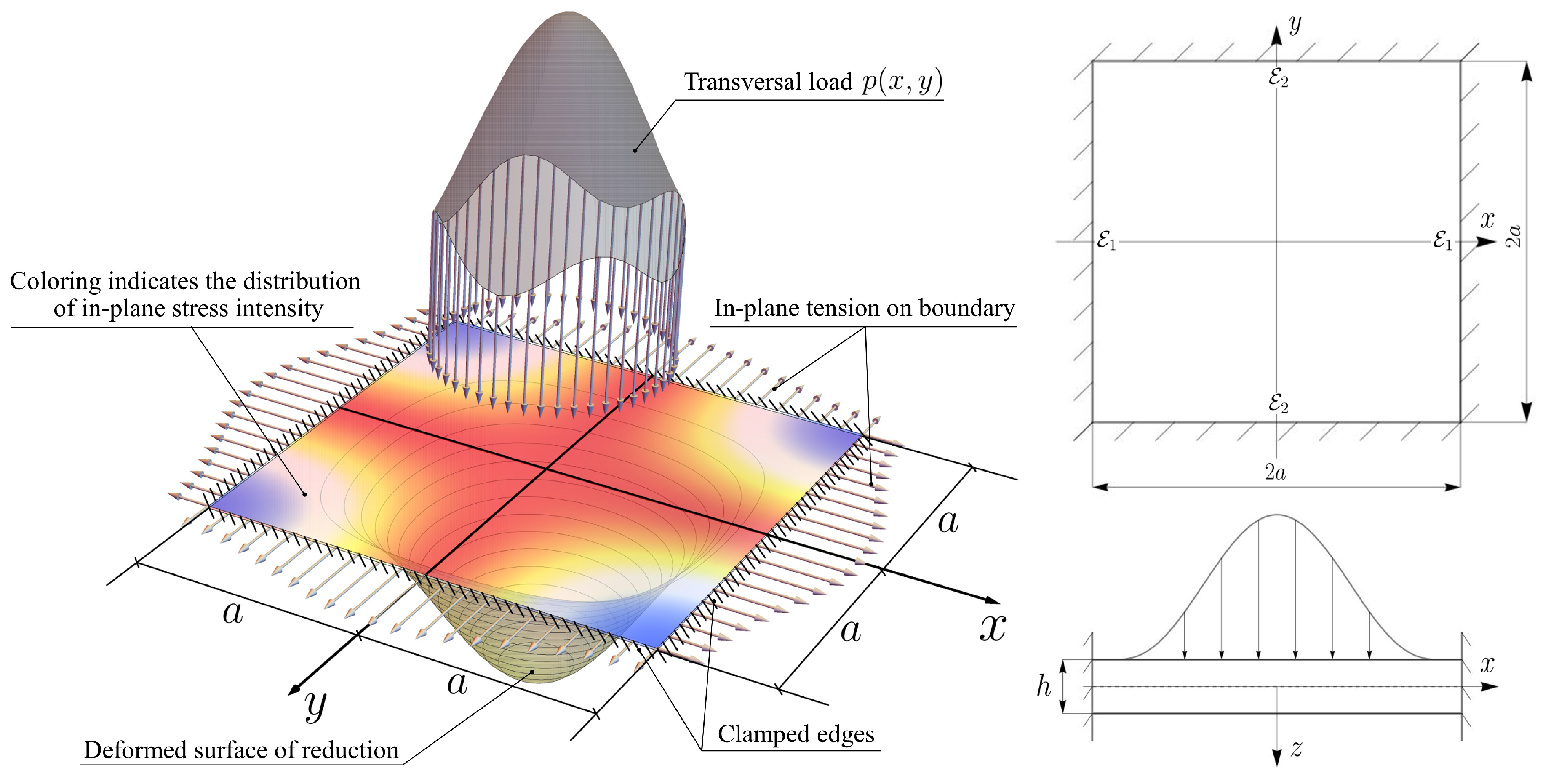
Figure 2.
Results for the model problem.
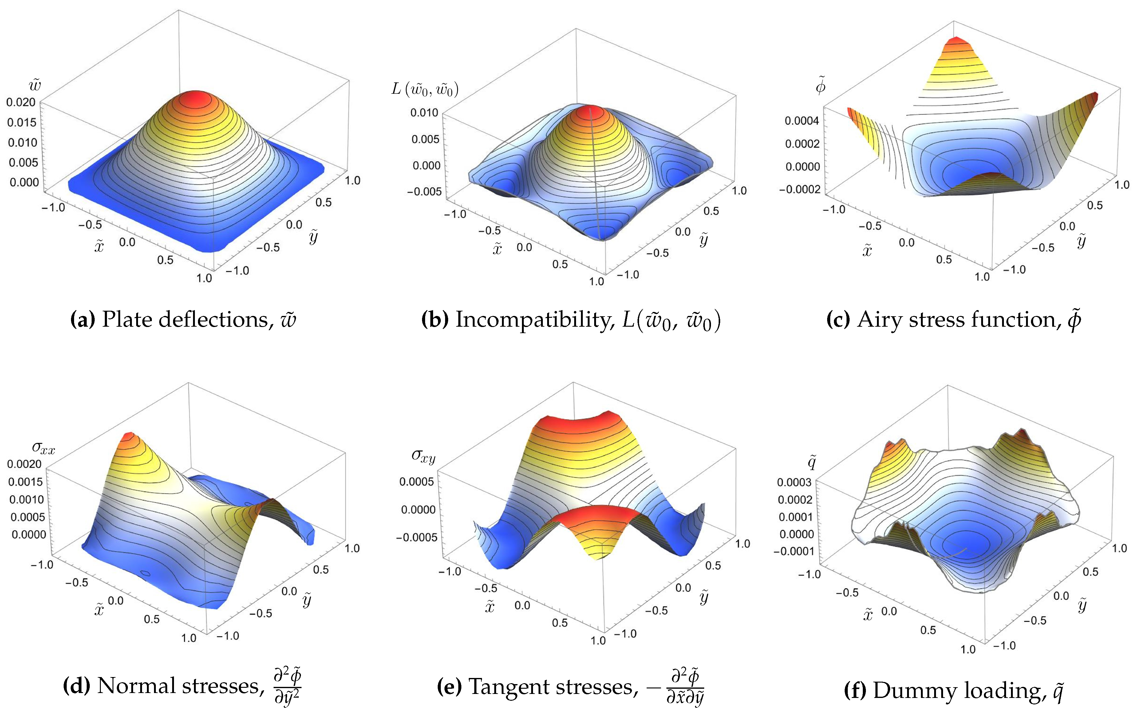
Figure 3.
Normalized auxiliary eigenfunctions and Cantor paring function diagram.
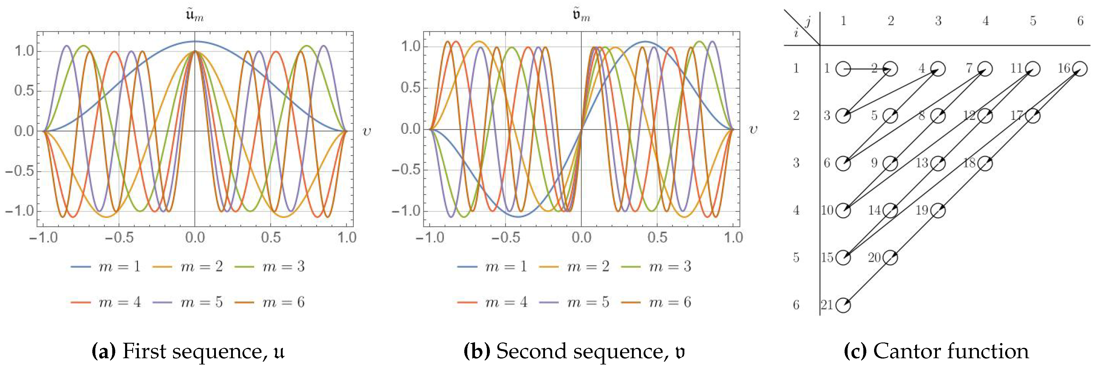
Figure 4.
Trial load functions and their reduced Fourier sums.
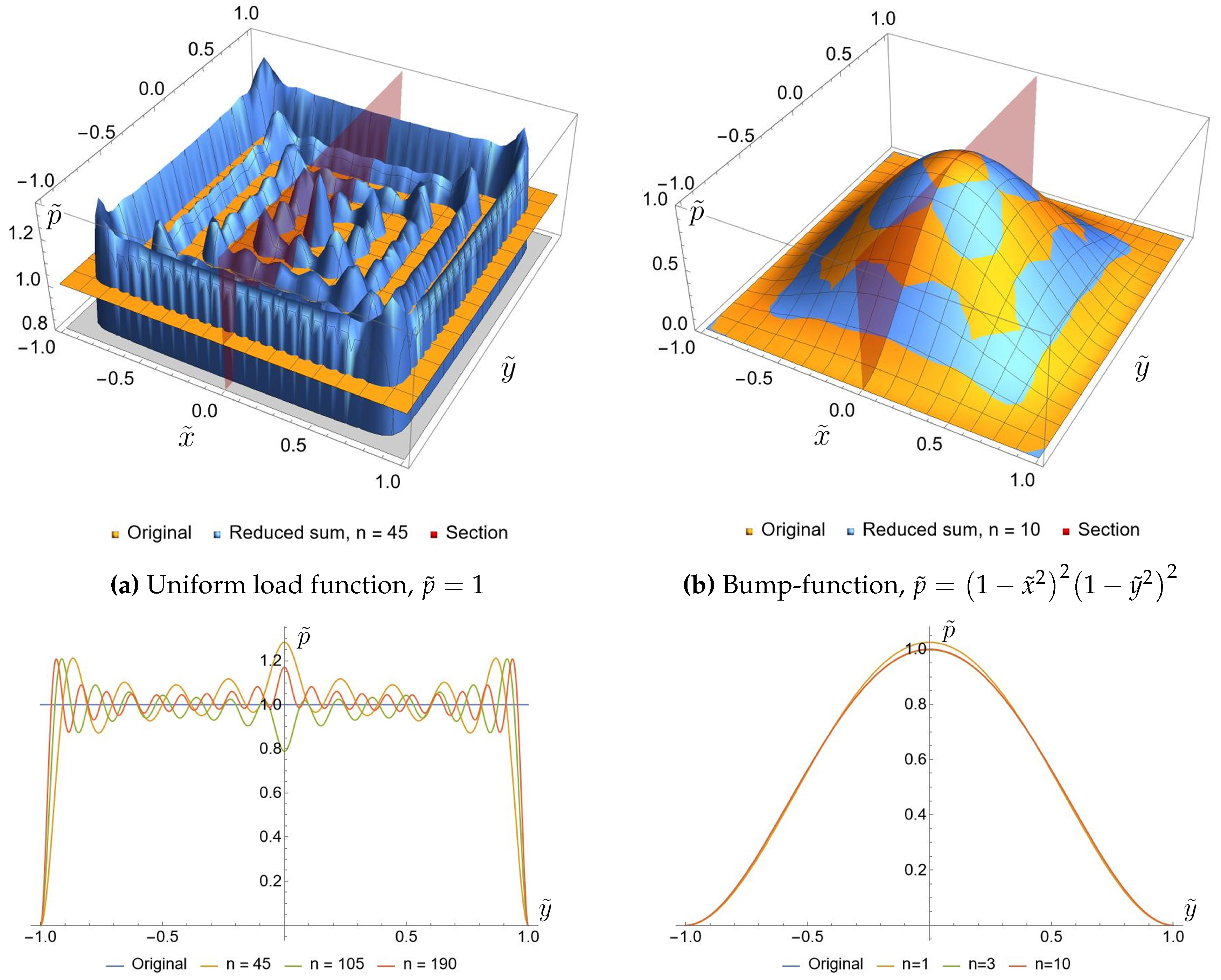
Figure 5.
Test solutions for plate under uniform load
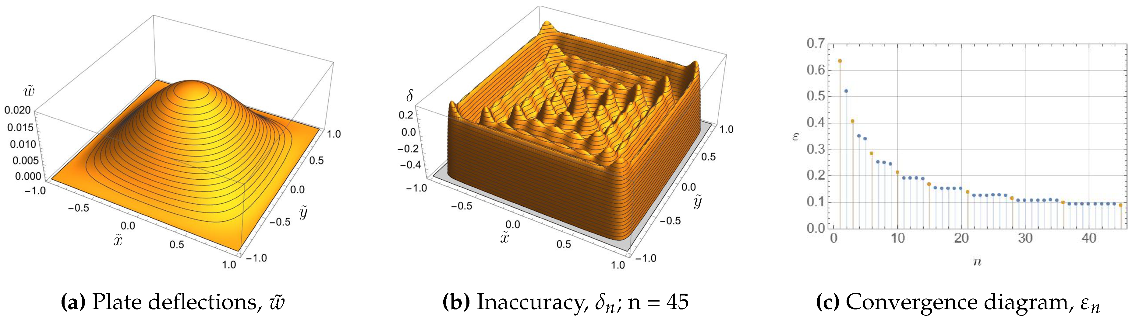
Figure 6.
Test solutions for plate under bump-function load
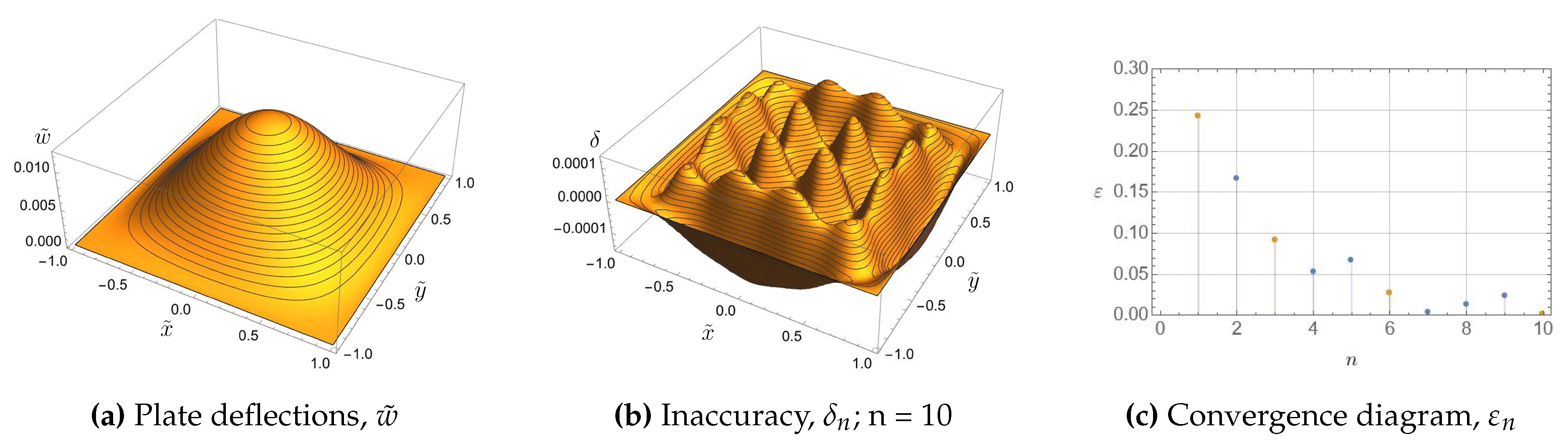
Figure 7.
Stress functions.
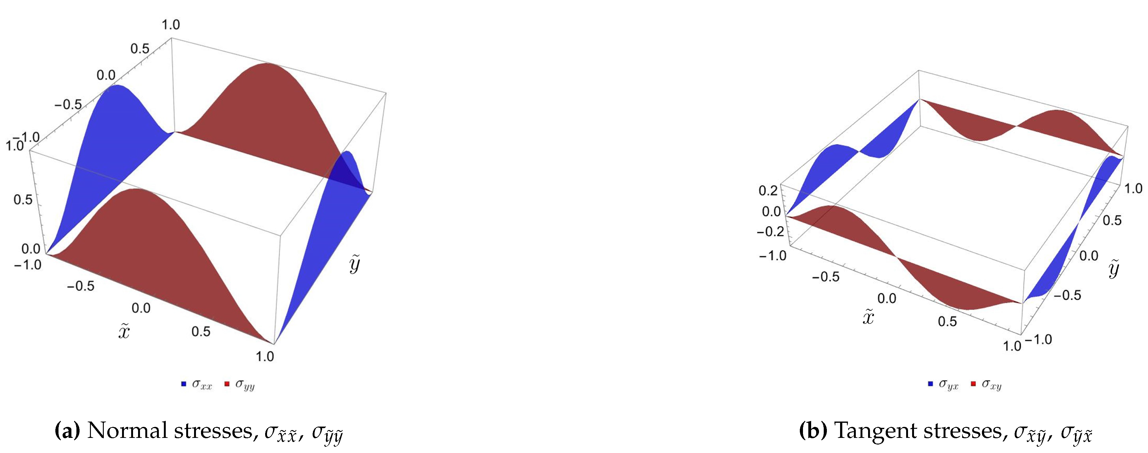
Figure 8.
The Airy function and corresponding stress distributions.
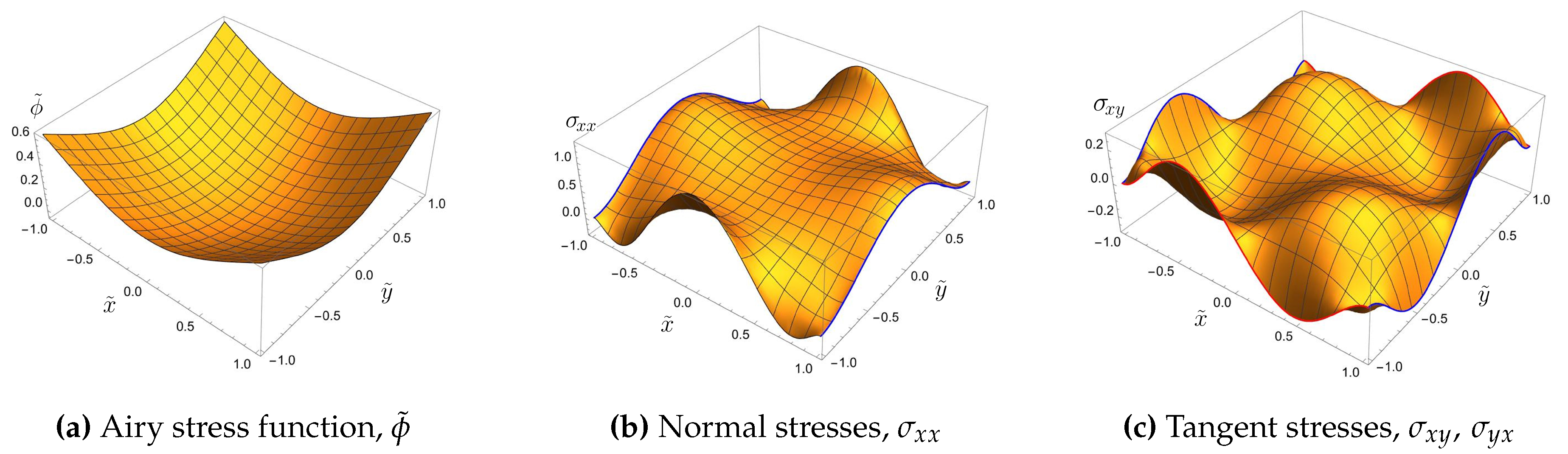
Figure 9.
Distributions for the elements of the solution at initial pressure 3 kPa without incremental loading.
Figure 9.
Distributions for the elements of the solution at initial pressure 3 kPa without incremental loading.
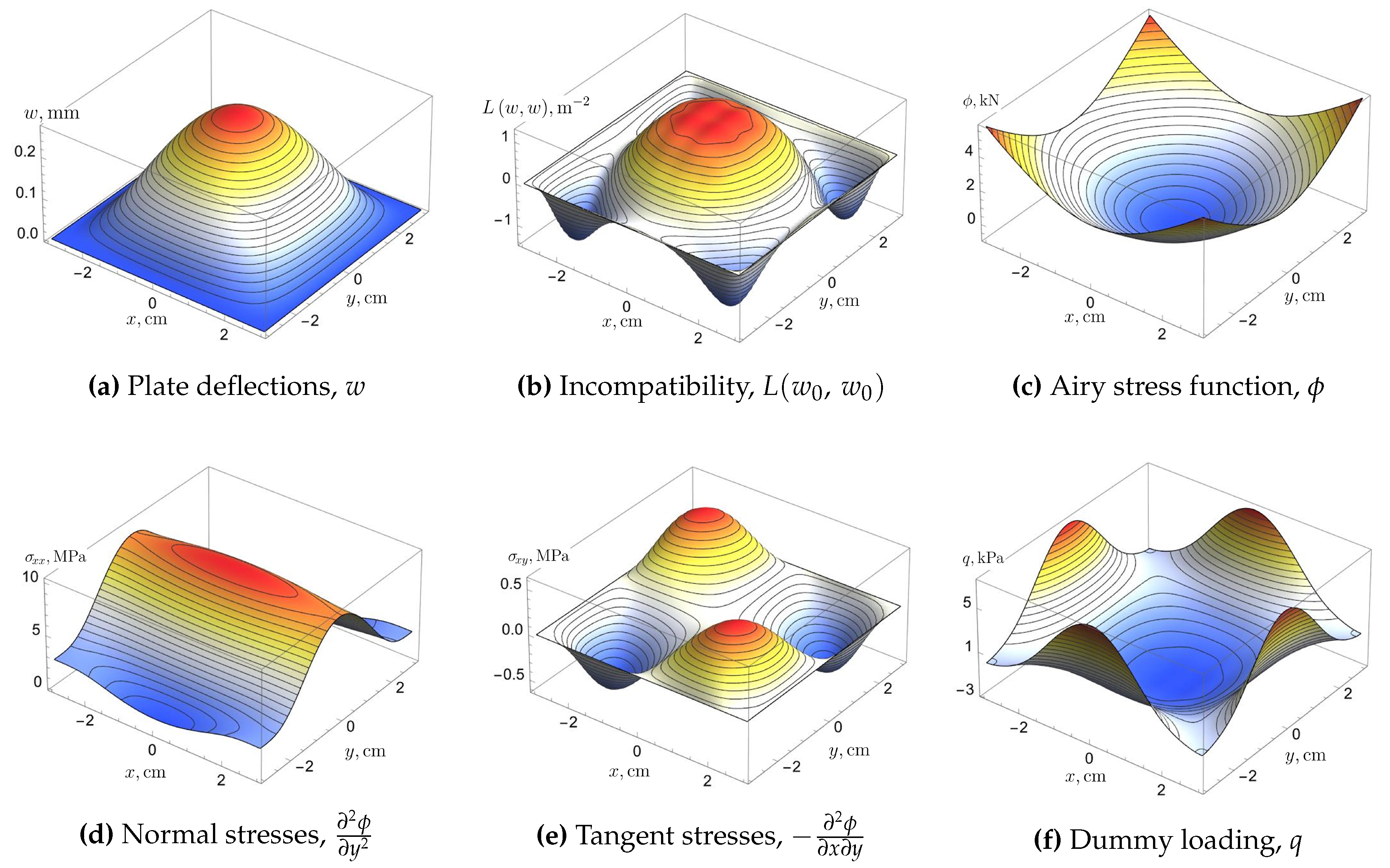
Figure 10.
Experimental and theoretical deflections of the plate central point in terms of contour line order (order increases by 1 when displacements increases by 266 nm).
Figure 10.
Experimental and theoretical deflections of the plate central point in terms of contour line order (order increases by 1 when displacements increases by 266 nm).
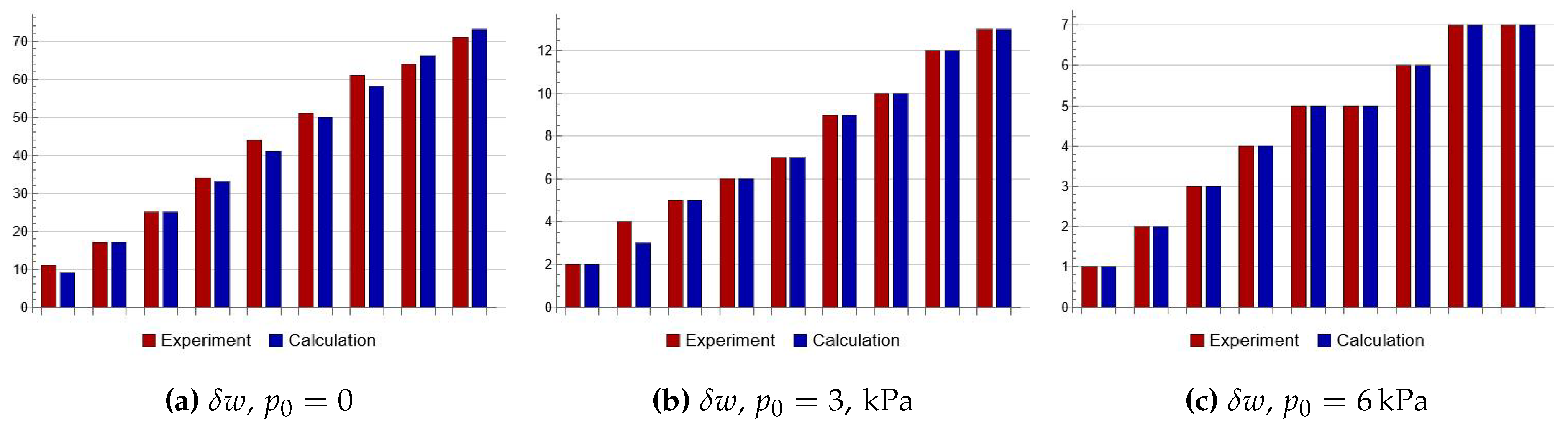
Figure 11.
Juxtaposition of theoretical and experimental deflections under different initial and incremental pressure. Step of contour lines is taken to be equal to half laser wavelength (266 nm).
Figure 11.
Juxtaposition of theoretical and experimental deflections under different initial and incremental pressure. Step of contour lines is taken to be equal to half laser wavelength (266 nm).
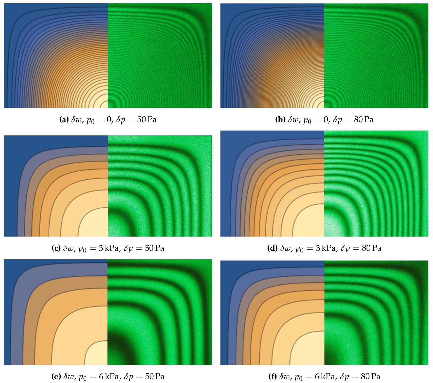

Table 1.
Eigenvalues .
| Eigenvalue number | Numerical solution | Approximation formula | Relative error |
|---|---|---|---|
| 1 | 2.36502 | 2.35619 | 0.00372 |
| 2 | 5.49780 | 5.49779 | |
| 3 | 8.63938 | 8.63938 | |
| 4 | 11.7810 | 11.7810 | |
| 5 | 14.9226 | 14.9226 |
Table 2.
Eigenvalues .
| Eigenvalue number | Numerical solution | Approximation formula | Relative error |
|---|---|---|---|
| 1 | 3.92660 | 3.92699 | 0.00010 |
| 2 | 7.06858 | 7.06858 | |
| 3 | 10.2102 | 10.2102 | |
| 4 | 13.3518 | 13.3518 | |
| 5 | 16.4934 | 16.4934 |
Table 3.
Components of auxiliary structures.
| Structure | Components expression |
|---|---|
| matrix | |
| matrix | |
| matrix | |
| matrix | |
| cubic matrix | |
| cubic matrix | |
| cubic matrix | |
| cubic matrix |
Table 4.
Components of auxiliary structures.
| Structure | Components Expression |
|---|---|
| vectors | |
| vector | |
| vector | |
| vector | |
| matrix | |
| matrix | |
| matrix | |
| matrix | |
| matrix | |
| cubic matrix | |
| cubic matrix |
Table 5.
Plate parameters.
| Length, cm | Thickness, m | Young Modulus, GPa | Poisson’s ratio |
|---|---|---|---|
| 6 | 184 | 128 | 0.35 |
Disclaimer/Publisher’s Note: The statements, opinions and data contained in all publications are solely those of the individual author(s) and contributor(s) and not of MDPI and/or the editor(s). MDPI and/or the editor(s) disclaim responsibility for any injury to people or property resulting from any ideas, methods, instructions or products referred to in the content. |
© 2024 by the authors. Licensee MDPI, Basel, Switzerland. This article is an open access article distributed under the terms and conditions of the Creative Commons Attribution (CC BY) license (http://creativecommons.org/licenses/by/4.0/).
Copyright: This open access article is published under a Creative Commons CC BY 4.0 license, which permit the free download, distribution, and reuse, provided that the author and preprint are cited in any reuse.


