Submitted:
20 January 2024
Posted:
22 January 2024
Read the latest preprint version here
Abstract
Background: Renal cancers are among the top ten causes of cancer specific mortality; of which the ccRCC subtype is responsible for most of the cases. Grading of ccRCC is important in determining the tumour aggressiveness and clinical management. Objectives: To predict the WHO/ISUP grade of ccRCC pre-operatively and characterise the heterogeneity of tumour subregions using radiomics and ML models including comparison with pre-operative biopsy determined grading in a subgroup. Methods: Data was obtained from multiple institutions across two countries from 391 patients with pathologically proven ccRCC. For analysis, the data were separated into 4 cohorts. Cohort 1 and 2 were data from the respective institutions from the two countries, cohort 3 was the combined data and cohort 4 data was a subset of cohort 1 where both biopsy and subsequent histology from resection (partial or total nephrectomy) was available. 3D image segmentation was done to derive a voxel of interest (VOI) mask. Radiomic features were then extracted from the contrast enhanced images and the data normalised. Correlation coefficients and XGBoost model were used to reduce the dimensionality of the features. Thereafter, 11 ML algorithms were implemented for the purpose of predicting the grade of ccRCC and characterising heterogeneity of subregions in the tumours; Results: For cohort 1, 50% tumor core and 25% tumor periphery exhibited best performance with an average AUC of 77.91% and 78.64% respectively. 50% tumor core had the highest performance in cohort 2 and cohort 3 with an average AUC of 87.64% and 76.91% respectively. Cohort 4 with 25% periphery showed an AUC of 95% and 80% for grade prediction using internal and external validation respectively while biopsy histology had an AUC of 31% for the prediction with final grade of resection histology as a reference standard; Conclusion: Radiomic signatures combined with ML have the potential to predict the WHO/ISUP grade of ccRCC with superior performance compared to pre-operative biopsy. Moreover, tumour subregions contain useful information that should be analysed independently when determining tumour grade. It is therefore possible to distinguish the grade of ccRCC pre-operatively to improve patient care and management.
Keywords:
clear cell renal cell carcinoma
; renal masses
; computed tomography
; radiomics
; machine learning
; tumour subregions
; tumour heterogeneity
; precision medicine
1. Introduction
Although being one of the top ten cancer killers [1] and the seventh most prevalent form of neoplasm in the developed world [2], kidney cancer has long gone unnoticed [1]. More than 90% of kidney cancer cases are renal cell carcinoma (RCC) [3], which refers to cancer that begin in the renal epithelium [4]. Despite all the advancements in care, renal cell carcinoma is a cunning neoplasm that accounts for about 2% of cancer diagnoses and fatalities worldwide [3], and is also the most dangerous renal malignancy despite all the improvements in management [5]. The cortex of the kidney, which is made up of the glomerulus, tubular apparatus, and collecting duct, is where the majority of RCCs develop [6]. In the fight against this aggressive malignancy, modifiable risk factors like smoking [7], obesity [7], uncontrolled hypertension [8], poor diet [9], alcohol assumption and occupational exposure [10] are top candidates for prevention efforts [11].
There are at minimum ten molecular and histological subtypes of this disease and ccRCC has been shown to be the most widespread and is liable for a majority of the cancer related deaths [4]. Clear cell RCC, a renal stem cell tumour, typically found in the proximal nephron and tubular epithelium [4], also known as conventional RCC [12], makes up to 80% of RCC diagnoses [13] and is more likely to hematogenously spread to the lungs, liver, and bones [14]. Most ccRCC tumours have the same primary driving characteristic, which is the loss of Von Hippel-Lindau (VHL) tumour suppressor gene function normally present throughout the tumour [15]. Clear cell RCC can be hereditary (4%) or random (>96%) [16]. Most of the familial ccRCCs are caused by a hereditary VHL mutation [11] and as a result of the abundance of cytoplasmic lipids in malignant cells, it exhibits the typical physical appearance of a well-circumscribed golden-yellow mass [17]. Microscopically, the tumour exhibits a complex vascular network [18] with tiny sinusoid-like capillaries dividing nests of malignant cells in addition to the typical clear cell morphology indicated by cytoplasmic lipid and glycogen build-up [19].
Since approximately a century ago, the grading of RCC has been acknowledged as a prognostic marker [20]. The tumour grade identifies whether cancer cells are regular or aberrant under a microscope. The more aberrant the cells seem and the higher the grade, the quicker the tumour is likely to spread and expand. Many different grading schemes have been proposed, initially focused on a collection of cytological characteristics and more recently on nuclear morphology. The nuclear size (area, major axis, perimeter), nuclear shape (shape factor, nuclear compactness), and nucleolar prominence characteristics are the main emphasis of the Fuhrman grading of renal cell carcinomas. Even though Fuhrman grading is said to be widely used in clinical investigations, its predictive value and reliability are up for discussion [21]. Fuhrman et al. [22] showed in 1982 that tumours of grades 1, 2, 3 and 4 had considerably differing metastatic rates. When grade 2 and 3 tumours were pooled into a single cohort, they likewise demonstrated a strong correlation between tumour grade and survival [22].
The International Society of Urologic Pathologists (ISUP) suggested a revised grading system for RCC in 2012 to address the shortcomings of the Fuhrman grading scheme [23]. This system is primarily based on the assessment of nucleoli: grade 1 tumours have inconspicuous and basophilic nucleoli at 400 times magnification; grade 2 tumours have eosinophilic nucleoli at 400 times magnification; grade 3 tumours have visible nucleoli at 100 times magnification; and grade 4 tumours have extreme pleomorphism or rhabdoid and/or sarcomatoid morphology [24]. For papillary and ccRCC, this grading system has been approved [23]. The World Health Organization (WHO) recommended the ISUP grading system at a consensus conference in Zurich; as a result, the WHO/ISUP grading system is currently applied internationally [24]. The abnormality of the tumour cells relative to normal cells is described by the tumour grade. It also characterises the tissues’ aberrant appearance when viewed under a microscope. The grade provides some insight into how cancer may act. A tumour classified as low grade is more likely to grow more slowly and spread less frequently than one with a high grade. So, grades 1 and 2 would be ranked as low grades and grades 3 and 4 as high-grade ccRCC.
Grading ultimately helps in the optimal management and treatment of tumours according to their prognostic behaviour concerning their respective grades. For instance, elderly or very sick patients who have small renal tumours (<4 cm) and high mortality rate, cryoablation, active surveillance or radiofrequency ablation may be considered to manage their conditions [25]. It is crucial to be aware that, confident radiological diagnosis of low-grade tumours in active surveillance can significantly impact clinical decisions hence eliminating the risk of overtreatment [26]. As ccRCC is the most prevalent subtype (8 in 10 RCCs) with the highest potential for metastasis, it requires careful characterisation [27]. High-grade cancers have a poorer prognosis, are more aggressive, have high-risk post-operative recurrence and may metastasise [26]. It is therefore very important to differentiate between different grades of ccRCC as high-grade ccRCC requires immediate and exact management. Precision medicine together with personalised treatment has advanced with the advent of cutting-edge technology hence clinicians are interested in determining the grade of ccRCC before surgery or treatment to enable them to advise on therapy and even predict cancer-free survival if surgery has been conducted.
The diagnosis of ccRCC grade is commonly done based on pre-operative and post-operative methods. One such pre-operative method is biopsy. However, the accuracy of a biopsy can be influenced by several factors, including the size and location of the tumour, the experience of the pathologist performing the biopsy, and the quality of the biopsy sample [28]. Due to sampling errors, a biopsy may not always provide an accurate representation of the overall tumour grade [29]. Inter-observer variability can also lead to inconsistencies in the grading process. This can be especially problematic for tumours that are borderline between two grades [30]. In some cases, a biopsy may not provide a definitive diagnosis as it only considers the cross-sectional area of the tumour compounded with the fact that ccRCC has high spatial and temporal heterogeneity [31] hence it is not representative of the entire tumour [32]. Biopsy also has a small chance of haemorrhage (3.5%) and a rare risk of track seeding (1:10,000) [33,34]. Due to the limitations highlighted for biopsy [35], radical or partial nephrectomy treatment specimens are usually used as definitive post-operative diagnostic tool for tumour grade. Partial or radical nephrectomy being the definitive therapeutic approach, a small but significant number of patients are subjected to unnecessary surgery even though their management may not require surgical resection. Nephrectomy also increases the possibility of contracting chronic renal diseases that may result in cardiovascular ailments [36]. Therefore, precise grading of ccRCC through non-invasive methods is imperative to improve the effectiveness and targeted management of tumours.
The assumption in most research and clinical practice is that solid renal masses are homogenous in nature or if heterogeneous, they have the same distribution throughout the tumour volume [37]. More recent studies [38] have highlighted that in some histopathologic classifications, different tumour subregions may have different rates of aggressiveness, hence heterogeneity plays a significant role in tumour progression. Ignoring such intra-tumoural differences may lead to inaccurate diagnosis, treatment and prognoses [39]. The biological makeup of tumours is complex and therefore shows spatial differences within their structures. These variations may be in the expression of the gene or microscopic structure [40]. The differences can be caused by several factors, among them being hypoxia which is the loss of oxygen in the cells and necrosis which is the death of cells. This is mostly synonymous with the tumour core. Likewise, high cell growth and tumour-infiltrating cells are factors associated with the periphery [41].
Medical imaging analysis has proven to be capable of detecting and quantifying the level of heterogeneity in tumours [42,43,44]. This ability enables tumours to be categorised into different subregions depending on the level of heterogeneity. In relation to tumour grading, intra-tumoural heterogeneity may prove useful in determining the subregion of the tumour containing the most prominent features that enable successful grading of the tumour. Radiomics, which is the extraction of high throughput features from medical images, is a modern technique that has been used in medicine to extract features which would not be otherwise visible using the naked eye alone [45]. It was first proposed by Lambin et al. [46] in 2012 to extract features taking into consideration the differences in solid masses. Radiomics eliminates the subjectivity in the extraction of tumour features from medical images as it works as an objective virtual biopsy [47]. There are quite a number of studies that have applied radiomics in the classification of tumour subtypes, grading and even the staging of tumours [48,49].
Over the years, there has been tremendous progress in the field of medical imaging with the advent of artificial intelligence (AI). AI has enabled analysis of tumour subregions in a variety of clinical tasks and using several imaging modalities such as CT and MRI [50]. However, these analyses have been limited to only a few types of tumours, particularly brain tumours [51] head and neck tumours [52] and breast cancers [53]. Until now there exists no study which has attempted to analyse the effect of intra-tumoural heterogeneity in the diagnosis, treatment and prognosis of renal masses and specifically ccRCCs. This rationale formed the basis of the present study on the effect of intra-tumoural heterogeneity on the grading of ccRCC. To our knowledge, no such study has been conducted before hence this becomes the first paper to comprehensively focus on tumour subregions in renal tumours for the prediction of tumour grade.
This research tested the hypothesis that radiomics combined with ML could significantly differentiate between high and low-grade ccRCC for individual patients. This study sought answers to two major questions which previous research has not been able to answer;
- Characterise the intra-tumoural heterogeneity in grading ccRCC.
- Compare the diagnostic accuracy of radiomics and ML to image-guided biopsy in determining the grade of renal masses using resection (partial or complete) histopathology as a reference standard.
2. Materials and Methods
2.1. Ethical Approval:
This study was approved by the institutional board and access to patients’ data was granted under the Caldicott Approval Number: IGTCAL11334 dated 21 October 2022. Informed consent for the research was not required as CT scan image acquisition is a routine examination procedure for patients suspected of having ccRCC.
2.2. Study Cohorts:
The retrospective multicentre study used data from three centres which are either in partnership or satellite hospitals of the National Health Service (NHS), in a well-defined geographical area of Scotland, United Kingdom. The institutions included Ninewells Hospital Dundee, Stracathro General Hospital and Perth Royal Infirmary Hospital. Data from the University of Minnesota Hospital and Clinic (UMHC) was also used [54,55]. Scan data was anonymised.
We accessed the Tayside Urological Cancers (TUCAN) database [56] for pathologically confirmed cases of ccRCC, between January 2004 and December 2022. A total of 396 patients with CT scan images were retrieved from the Picture Archiving and Communication System (PACS) in DICOM format. This data formed our first cohort (cohort 1). Retrospective-based analysis for pathologically confirmed ccRCC image data following partial or radical nephrectomy from UMHC stored in a public database [57] (accessed on 21 May 2022) was done and is referred to as cohort 2. The database was queried for data between 2010 and 2018. A total of 204 patients with ccRCC CT scan images were collected.
The inclusion criteria for the study were as follows:
- Availability of protocol-based pre-operative contrast-enhanced CT scan in the arterial phase.
- Confirmed histopathology from partial or radical nephrectomy with grades reported by a uro-pathologist according to WHO/ISUP grading system.
- CT scans with data to achieve a working acquisition for 3D image reconstruction.
The exclusion criteria were:
- Patients with only biopsy histopathology.
- Metastatic clear cell renal cell carcinoma (mccRCC).
- Patients with bilateral or ipsilateral multiple tumours primarily due to the database’s ambiguity in distinguishing between the tumours exact grades.
2.3. CT Acquisition Technique:
The patients in cohort 1 were examined using up to five different CT helical/spiral scanners including GE Medical Systems, Philips, Siemens, Canon Medical Systems and Toshiba with 512-row detectors. The detectors were also of different models including Aquilion, Biograph128, Aquilion Lightning, Revolution EVO, Discovery MI, Ingenuity CT, LightSpeed VCT, Brilliance 64, Aquilion PRIME, Aquilion Prime SP, Brilliance 16P. The slice thicknesses were: 1.50, 0.63, 2.00, 1.25 and 1.00 mm. The arterial phase of the CT scan obtained 20-45 seconds after contrast injection was acquired using the following method: intravenous Omnipaque 300 contrast agent (80-100 mls), 3 ml/s contrast injection for the renal scan, 100-120 kVp with an X-ray tube current of 100-560 mA depending on the size of the patient. For the UMHC dataset refer to [54,55].
2.4. Data Curation:
The procedure used for data collection of each patient comprised of multiple stages: accessing the Tayside Urological Cancers database, identification of patients using a unique identifier (community health index number or CHI number), review of the medical records of the cohort, CT data acquisition, annotation of the data and finally quality assurance. Anonymised data for cohort 1 was in DICOM format. For each patient, duplicated DICOM slices were removed since inconsistency in a slice has incremental effects on how an image can be processed.
Image quality is an important factor in Machine learning modelling [58]. We went through the images to remove low quality scans such as scans with poor resolution, low contrast and those with significant Poisson noise. These factors can be due to low-dose scanning, patient motion, technical issues, and ring and metal artefacts [59]. Figure 1 represents a flowchart showing the exclusion and inclusion criteria of patients and their categorisation. Tumour grades 1 and 2 were labelled as low grades whereas grades 3 and 4, were classified as high grades. This is because the clinical management for grades 1 and 2 are more or less similar, and similarly for grades 3 and 4.
2.5. Tumour Sub-volume Segmentation Technique
In cohort 1, CT image slices for each patient were converted to 3D NIFTI (Neuroimaging Informatics Technology Initiative) format using Python programming language version 3.9 [60] and loaded into 3D Slicer version 4.11.20210226 software [61,62] for segmentation. Manual segmentation was performed on the 3D image delineating the edges of the tumour slice by slice to obtain the VOI. To make the image smoother the median [63,64,65,66,67] smoothing method was used; as it maintains image features and preserves edges and other important details in the image. The kernel size of the smoothing was 3mm i.e., 3x3 pixel.
The above procedure was performed by a blinded investigator (A.J.A.) with 14 years of experience in interpreting medical images who was unaware of the final pathological grade of the tumour. Confirmatory segmentation was done by another blinded investigator (A.J.) with 12 years of experience in using medical imaging technology on 20% of the samples to ascertain the accuracy of the first segmentation. Thereafter, the segmentations were assessed and ascertained by an independent experienced urological surgical oncologist (G.N.), taking into consideration radiology and histology reports. The gold standard pathology diagnosis was assumed to be partial or radical nephrectomy histopathology.
For cohort 2, Heller et al. [54] did the segmentation by following a set of instructions including ensuring that the images of the patients contain the entire kidney, drawing a contour which includes the entire tumour capsule and any tumour or cyst but excluding all tissues other than renal parenchyma and drawing a contour that includes the tumour components but excludes all kidney tissues. In the present study only the delineation of kidney tumours was done by Heller et al. [54] was considered. To perform delineation a web-based interface was created on the HTML5 Canvas that allowed drawing contours on the images freehand. The image series were subsampled in the longitudinal direction regularly so that the number of annotated slices depicting a kidney was about 50% compared to the original. Interpolation was also performed. More information on the segmentation of the cohort 2 dataset can be found in this report [54].
The result of the segmentation for both cohorts 1 and 2 was a binary mask of the tumour. In the present study, the tumour was divided into different subregions based on the geometry of the tumour i.e., periphery and core. The periphery refers to regions towards the edges of the tumour whereas the core represents regions close to the centre of the tumour. The core was obtained by extracting 25%, 50% and 75% of the binary mask from the centre of the tumour while, the periphery was generated by extracting 25%, 50% and 75% of the binary mask starting from the edges of the tumour to form a rim as a hollow sphere. A detailed visual description is shown in Figure 2, Figure 3 and Figure 4. Mask generation was done using a Python script which automatically generated the subregions through image subtraction techniques.
2.6. Radiomics Feature Computation
Similar to our previous research [48], texture descriptors of the features were computed using the PyRadiomics module in Python 3.6.1. [68]. PyRadiomics is a module that has attempted to implement a standardised way of extracting radiomic features from medical images avoiding inter-observer variability [69]. The parameters used in Pyradiomics were: Minimum region of interest (ROI) Dimension of 2, pad distance was set to 5, Normalisation False and Normaliser scale was 1. There was no removal of outliers, no resample pixel spacing and no pre-cropping of the image. SitkBSpline was used as the interpolator with the bin-width being set to 20.
On average, Pyradiomics generates approximately 1500 features for each image. Pyradiomics enables the extraction of 7 feature classes per 3D image. This was done with the 3D image in NIFTI format and the binary mask image. The feature categories extracted were as follows: First-order (19 features), Gray-Level Co-occurrence Matrix (GLCM) (24 features), Gray-Level Run-Length Matric (GLRLM) (16 features), Gray-Level Size-Zone Matrix (GLSZM) (16 features), Gray-Level Dependence Matrix (GLDM) (14 features), Neighbouring Gray-Tone Difference Matrix (NGTDM) (5 features) and the 3D Shape features (16 features). These features compute the texture intensity and the way they are spread in the image [69].
In a previous study [48] it was shown that a combination of the original feature classes and filter features improved model performance significantly. We therefore extracted the filter class features in addition to the original features. These filter classes included: Local Binary-Pattern (LBP-3D), Gradient, Exponential, Logarithm, Square-Root, Square, Laplacian of Gaussian (LoG) and Wavelet. The filter features are applied to every feature in the original feature classes for instance first-order statistic feature class has 19 features it follows that and it will have 19 LBP filter features. The filter class feature is named according to the name of the original feature and the name of the filter class. [69].
2.7. Feature Processing and Feature Selection
The features extracted using PyRadiomics were standardised to assume a standard distribution. The scaling was performed using the Z score Equation (1) for both the training and testing dataset independently, however using the mean and standard deviation generated from the training set. This was done to avoid leakage of information while also eliminating bias from the model. All the features were transformed in such a way that they had the properties of a standard normal distribution with mean ()=0 and standard deviation ()=1.
Where,
- Z: Value after scaling the feature.
- x: The feature.
- : Mean of all the features in training set.
- : Standard deviation of the training set.
Normalisation reduces the effect of different scanners, as well as any influence that intra-scanner differences may introduce in textural features with improved correlation to histopathological grade [70]. The ground truth labels were denoted as 1 for high grade and 0 for low grade for the purpose of enabling the ML models to understand the data. Machine learning models usually encounter the "curse of dimensionality" in the training dataset [71], when the number of features in the dataset is greater than the number of samples. We therefore applied two feature selection techniques in an attempt to reduce the number of features and retain only those features with the highest importance in predicting the tumour grade. First, the inter-feature correlation coefficient was computed and where two features had a correlation coefficient greater than 0.8, one of the features was dropped. Thereafter, we used the XGBoost algorithm to further select the features with the highest importance for the model development.
2.8. Subsampling
In ML the spread of data among different classes is an important consideration before developing a ML model. An imbalance in data may lead the model being biased towards the majority class, instead of learning the features of the data, the model will be “cramming” making the model inapplicable in real-life scenarios. In this research our data samples were imbalanced, and we therefore applied the synthetic minority oversampling technique (SMOTE) to balance the data. Care should be taken when using SMOTE as it should only be applied in the training set and not the validation and testing set, if this were done there is a possibility for the model to gain an improvement in operational performance due to data leakage [72,73].
2.9. Statistical Analysis
Common clinical features in this research were analysed using the SciPy package. Comparisons were done on the age, gender, tumour size and tumour volume against the pathological grade. The Chi-square test () was used to compare the associations between categorical groups. Chi-square test is a non-parametric test used when the data does not follow the assumptions of parametric tests, such as the assumption of normality in the distribution of the data. The student t-test is a popular statistical tool used when assessing the difference between two population means for continuous data. It is normally used where the population follows a normal distribution and the population variance is unknown. In cases where statistical significance between the clinical data was obtained, the point-biserial correlation coefficient (rpb) was used to further confirm the significance. Pearson correlation coefficient was used to measure the linear correlation in the data between the radiomic features. The coefficient value ranges between -1 to 1, with one signifying a strong positive correlation.
McNemar’s statistical test which is a modified Chi-square test, was used in the research to test if the difference between false negative (FN) and false positive (FP) was statistically significant. It was calculated from the confusion matrix using the stats module in the SciPy library. The Chi-square test for randomness was used to test whether the model predictions were different from random. The dice similarity coefficient was used to determine the inter-reader agreement for the segmentations. All statistical tests assumed at a significant level of p<0.05 i.e., the null hypothesis was rejected when the p-value was less than 0.05. The radiomic quality score (RQS) was also calculated to evaluate whether the research followed the scientific guidelines of radiomic studies. The study followed the established guidelines of transparent reporting of a multi-variable prediction model for individual prognosis or diagnosis (TRIPOD) [74].
2.10. Model Construction, Validation and Evaluation
Several models were implemented to predict the pathological grade of ccRCC using the WHO/ISUP grading system as a gold standard. The models were constructed for cohorts 1, 2 and the combined cohort. The ML models included the Support Vector Machine (SVM) (kernel=rbf, probability=True, random_state=42, gamma=0.2,C=0.01), Random Forest (RF) (n_estimators=401, random_state=42, max_depth=3), Extreme Gradient Boosting (XGBoost/XGB) (random_state=42, learning_rate=0.01, n_estimators=401, gamma=0.52), Naïve Bayes (NB) GaussianNB(), Multi-layer Perceptron Classifier (MLP) (hidden_layer_sizes=(401,201), activation=relu, solver=adam, max_iter=5), Long Short-Term Memory (LSTM) (loss=binary_crossentropy,optimizer=Adam lr=0.01, metrics=accuracy, epochs=1000,batch_size=16), Logistic Regression (LR) (random_state=42, max_iter=4), Quadratic Discriminant Analysis (QDA) (reg_param=0.05), Light Gradient Boosting Machine (LightGBM/LGB)(random_state=42,n_estimators=9), Category Boosting (CatBoost/CB) (random_state=42, verbose=False, iterations=50) and Adaptive Boosting (AdaBoost/ADB) (base_estimator=rf, n_estimators=201, learning_rate=0.01, random_state=42).
In total 231 distinct models were constructed i.e., 11 models for each of the three cohorts and each tumour subregion (11 x 3 x 7). For validation, the dataset was divided into training and testing sets. For each cohort 67% of the data was used for training and 33% was left out for testing. This formed part of our internal validation. Besides that, we took cohort 1 as the training set and cohort 2 as the testing set and vice versa. This formed part of our external validation. It should be noted that although cohort 1 has been taken to be analogous to a “single institution” dataset, it was obtained from multiple centres and its comparison with cohort 2 was for external validation of the predictive models.
A subset of cohort 1 consisting of patients who underwent both CT-guided percutaneous biopsy and nephrectomy (28 samples) were evaluated using two separate ML algorithms. One model was trained on cohort 1, but excluding the 28 patients who had both procedures conducted. While the second model was trained on cohort 2 which acted as an external validator. The classifiers and subregions were determined for the two best-performing classifiers and the three best-performing tumour regions. The objective for this was to assess the accuracy of tumour grade prediction from biopsy results when compared to ML prediction using partial or total nephrectomy histopathology as a gold standard. These 28 samples were referred to as cohort 4. In situations where biopsy results were indeterminate for a specific tumour, we concluded its final pathological grade as the opposite of the nephrectomy grade for that tumour i.e., if the nephrectomy outcome was high grade but the biopsy result was indeterminate, we conclude that the biopsy has indicated low grade for the purpose of analysis. Evaluation of the model performance was done using a number of metrics including Accuracy, Specificity, Sensitivity, Area Under the Curve of the Receiver Operating Characteristic curve (AUC-ROC), Mathew’s correlation coefficient (MCC), F1 Score, McNemar’s test and Chi-squared test.
3. Results
3.0.1. Study Population and Statistical Analysis
In cohort 1, after the implementation of the inclusion and exclusion criteria, we had 187 patients with pathologically proven ccRCC. Of the 187, 80 patients were low grade and 107 were of high grade ccRCC. The mean age was 59.05 and 64 for low and high-grade tumours respectively. Gender-wise 65.78% of patients were male with 34.22% female. The average tumour size and tumour volume are 4.32 cm and 75.8 cm3 respectively for low grade. Likewise, for high grade, it is 6.033 cm and 203.74 cm3 respectively. For cohort 2, the dataset met all the inclusion and exclusion criteria hence no sample was eliminated. The mean age was 57.17 for low grade and 63.68 for high grade. The average tumour size and tumour volume were 3.89 cm and 51.44 cm3 low grade. For high grade, it was 6.81 cm and 235.26 cm3 respectively. In terms of gender 65.69% were male and the rest were female.
Except for gender; differences in average age, tumour size, and tumour volume were statistically significant in cohorts 1, 2 and the combined. However, using the point-biserial correlation coefficient (rpb) by comparing the correlation between the best model prediction and the clinical features, there was no statistical significance found. Refer to Table 1 and Table 2 for sample size distribution and patients’ characteristics and analysis respectively. The Dice similarity coefficient score was 0.93 which showed that there was a good inter-reader agreement for tumour segmentation. The entire data set RQS was found to be 61.11% signifying that the research followed scientific radiomic guidelines. For the RQS rubric refer to https://www.radiomics.world/rqs2 [74].
3.0.2. Feature Extraction, Pre-processing and Selection
A total of 1875 features were extracted using the PyRadiomics library. There were no null values in the data as it is crucial in the context of ML to handle these values to avoid errors or undefined results. Pearson correlation coefficient and eXtreme Gradient Boosting algorithm were used to reduce the number of features to only the best features. The number of features selected (FS) varied from one dataset to the other.
3.0.3. Model Validation and Evaluation
Internal Validation
Cohort 1
From the models that we developed the CatBoost classifier performed the best for the majority of the tumour subregion models with its best classifier having an AUC of 85% in the 100% tumour. When the tumour subregion was considered 50% tumour core and 25% tumour periphery exhibited the best performance with an averaged AUC of 77.91% and 78.64% respectively. When the models were averaged the best classifier was CatBoost with an AUC of 80.00% (80.67%+79.33%)/2. Refer to Table 3 and Table 4 for cohort 1 results.
Cohort 2
The best-performing model in the cohort 2 dataset was the CatBoost classifier with the best performance in the 50% tumour periphery having an AUC of 91%. In terms of tumour subregion, the 50% tumour core had the highest average AUC of 87.64%. When the models were averaged the best classifier was CatBoost with an AUC of 86.50% (87%+86%)/2. Refer to Table 5 and Table 6 for cohort 2 results.
Cohort 3
When NHS and UMHC data are combined, the model giving the highest AUC is the 50% tumour core CatBoost classifier and the 75% tumour periphery RF classifier with AUC of 80% for both. 50% tumour core was the best region with an average an AUC of 76.91%. When the models were averaged the best two classifiers were RF and CatBoost with an AUC of 77.33% (76.33%+78.33%)/2 and 77.00% (77.33%+76.67%)/2 respectively. Refer to Table 7 and Table 8 for cohort 3 results.
External Validation
Cohort 1
When cohort 2 is used as the training set and cohort 1 is predicted on its models, the best performing model is the QDA 25% tumour periphery classifier with an AUC of 71%. For tumour subregion 25% tumour periphery was the best with an average AUC of 65%. When the models were averaged the best classifier was QDA with an AUC of 67.67% (67.33%+68%)/2. Refer to Table 9 and Table 10 for the results.
Cohort 2
When cohort 1 is used as the training set and cohort 2 as the testing set, the best performing model was the SVM 50% tumour core classifier with an AUC of 77%. For tumour subregion 50% tumour core was the best with an average AUC of 74.18%. When the models were averaged the best classifier was RF with an AUC of 74.83% (74.33%+75.33%)/2. Refer to Table 11 and Table 12 for the results.
3.0.4. Comparison Between Biopsy and Machine Learning Classification
When biopsy classification results on the 28 samples separated from NHS dataset are compared to ML. Machine learning exhibited the highest AUC of 95% and 80% for internal and external validation respectively using CatBoost classifier. This was better than AUC of 31% found from biopsy in terms of correctly grading renal cancer as shown in Figure 5. Most statistics can be found from the Table 13 and Table 14.
4. Discussion
Clear cell renal cell carcinoma is the most common subtype of renal cell carcinoma and is responsible for a majority of renal cancer-related deaths. It makes up to 80% of RCC’s diagnosis [5] and is more likely to metastasise to other organs [14]. Important diagnostic criteria that must be derived include tumour grade, tumour stage, and the histological type of the tumour. For most cancer patients, histological grade is a crucial predictor of local invasion or systemic metastases and may affect how well they respond to treatment. To define the extent of the tumour; tumour staging-based clinical assessment, imaging investigations, and histological assessment are required. A greater comprehension of the neoplastic situation and awareness of the limitations of diagnostic techniques are made possible by an understanding of the procedures involved in tumour diagnosis, tumour grading, and tumour staging.
The grading of RCC was determined as a prognostic marker more than a hundred years ago [20]. It identifies a tumour as being either regular or aberrant when observed under a microscope, hence it is one of the factors that determines the ability of cancer to grow and spread to other adjacent cells. To accurately grade a tumour, several grading schemas have been applied, from which the WHO/ISUP and the Fuhrman grading systems have been the most popular and widely accepted. Previously, grading had been focused on a collection of cytological characteristics of the tumour, however; more recently nuclear morphology has been a major area of focus. The Fuhrman grading system has been used for quite a long time [75] with its worldwide adoption being in 1982 [22]. Nuclear size, nuclear shape and nucleolar prominence are major characteristics associated with the Fuhrman grading system [75,76]. Fuhrman et al. [22], demonstrated in 1982 that grade 1, 2, 3 and 4 tumours had considerably different rates of metastasis, likewise they also demonstrated that when grade 2 and 3 were pooled together there was a significant and strong correlation between tumour grade and survival [22].
Despite these seemingly encouraging findings, there are several methodological issues with the Fuhrman study. Its reliance on retrospective data collected over a 13-year period raises questions about potential biases [20]. The system’s dependency on a small sample size of only 85 cases may also make its conclusions less generalisable [20,75]. The inclusion of several RCC subtypes without subtype-specific grading in the study leaves out the possibility of variances in tumour behaviour [20,75,77]. It is difficult to grade consistently and accurately due to the complexity of the criteria, which calls for the evaluation of three nuclear factors simultaneously i.e., nuclear size, nuclear irregularity and nucleolar prominence [75,77] resulting in poor inter-observer reproducibility and interpretability. The lack of guidelines that can be utilised to assign weights to the different parameters when they are discordant to achieve a final grade makes the Fuhrman system even more controversial [75,76]. Furthermore, the shape of the nucleus was not well defined for different grades [75]. Grading discrepancies are a result of conflict between the grading criteria and a lack of direction for resolving them [20,23,77]. Additionally, imprecise standards for nuclear pleomorphism and nucleolar prominence adversely affect pathologists’ classifications resulting in increased variability [75]. Even if a tumour is localised, grading according to the highest-grade area could result in an overestimation of tumour aggressiveness [20,75]. This system’s inconsistent behaviour and poor reproducibility [77] raises questions regarding its dependability and potential effects on patient care and prognosis [78]. Flaws with inter-observer repeatability [78,79] and the fact that the Fuhrman grading system is still widely used despite these flaws, shows there is a need for more research and better grading methods.
An extensive and cooperative effort resulted in the development of the ISUP grading system for renal cell neoplasia as an alternative to the Fuhrman grading system in 2012 [75,77]. The system was ratified and adopted by the WHO in 2015 and renamed as the WHO/ISUP grading system [20,24]. As opposed to the Fuhrman grading system, the ISUP system focuses on the nuclei prominence alone as the sole parameter that should be utilised when identifying tumour grade. This reduction in rating parameters has led to better grade distinction and increased predictive value. This has also eliminated the controversy around reproducibility that had been identified in the Fuhrman grading system. Previous studies have shown that there is a clear separation between grades 2 and 3 in the WHO/ISUP grading system which was not the case with the Fuhrman system. Indeed, Dugher et al. [23] in their study highlighted that there was a downgrade of Fuhrman grades 2 and 3 to grades 1 and 2 respectively in the WHO/ISUP system. This indicates that besides the overlap of grades in Fuhrman, there was also an overestimation of grades, a problem that has been rectified with the WHO/ISUP grading system [23,49,80]. The WHO/ISUP grading system has been highly associated with the prognosis of patients [81].
A pre-operative imaging-guided biopsy is a diagnostic tool that is used to identify the tumour grade. However, there are inherent problems that have been identified with this approach. The fact that this is invasive in nature and would mean discomfort and may also cause other complications to patients when the procedure is performed [35,82]. Therefore, non-invasive testing, imaging and clinical evaluations may be necessary to confirm the presence of ccRCC and its grade without having to undergo such procedure. Radiomics has gained traction in clinical practice in recent years, becoming a buzzword since 2016 [45]. It refers to the extraction of high-dimensional quantitative image features in what is known as image texture analysis, and it describes the pixel intensity in medical images such as X-ray images, CT, MRI, CT/PET, CT/SPECT, US and Mammogram scans. It has been applied in a number of studies for the diagnosis, grading and staging of tumours. Machine learning is one of the major branches of AI and a method that is used to train on a set of known data and then tested on unknown data. It is an attempt to make machines more intelligent by determining spatial differences in data that would have been otherwise difficult for a human being to decipher. It has been used in combination with texture analyses, particularly in tumour classification, grading and staging. It is capable of learning and improving through the analysis of image textural features thereby resulting in higher accuracy than native methods [83].
Heterogeneity within tumours is a significant predictor of outcomes, with greater diversity within the tumour potentially linked to increased tumour severity. The level of tumour heterogeneity can be represented through images known as kinetic maps which are simply signal intensity time curves [84,85,86]. Studies [87,88] that have utilised these maps end up averaging the signal intensity features throughout the solid mass hence regions with different levels of aggressiveness end up contributing equally in determining the final features. This leads to a loss of information about the correct representation of the tumour [89,90]. In some studies, there have been attempts to preserve intra-tumoural heterogeneity by extracting the features at the periphery and the core, and analysing them separately [42,43,44,88]. However, this is still not enough as information in other subregions of the tumour is not considered.
In this research, we undertook to investigate the influence of intra-tumoural subregion heterogeneity and biopsy on the accuracy of grading ccRCC. A total sample size of 391 patients with pathologically proven ccRCC from two broad data sets was used. The objective of the study was therefore to study the impact of intra-tumoural heterogeneity in grading ccRCC and compare and contrast ML and AI-based methods combined with CT radiomics signatures to biopsy, partial and radical nephrectomy in determining the grade of ccRCC. Finally, the research was to investigate the possibility of CT radiomics ML analysis to be used as an alternative to and thereby replacing the conventional WHO/ISUP grading system in the grading of ccRCC.
The experimental findings from our research have highlighted various aspects of the discussion. From the results, it was found that age, tumour size and tumour volume were statistically significant for cohorts 1, 2 and 3. However, for cohort 4 none of the clinical features were found to be significant. Upon further analysis of the statistically significant clinical features using the point-biserial correlation coefficient (rpb), none of the features were verified as significant. Moreover, 50% core tumour subregion was identified from the results as the best tumour subregion with the highest averaged performance for the models in cohorts 1, 2 and 3 with average AUCs of 77.91%, 87.64% and 76.91% respectively. It is worth noting that 25% periphery tumour subregion experienced an increase in its average performance for cohort 1 having an AUC of 78.64%, however, this result was not statistically different from that of 50% core and it failed to register the best performances in the other cohorts.
Among the 11 classifiers, the CatBoost classifier was the best model in all three cohorts with an average AUC of 80.00%, 86.50% and 77.00% for cohorts 1, 2 and 3 respectively. Likewise, the best performing distinct classifier per cohort was CatBoost with an AUC of 85% in 100% core, 91% in 50% periphery and 80% in 50% core for cohorts 1, 2 and 3 respectively. On external validation, cohort 1 validated on cohort 2 data had the highest performance in 25% periphery with the highest AUC of 71% and the best classifier being QDA. Conversely, cohort 2 validated on cohort 1 data provided the best performance in the 50% core with an AUC of 77% and the best classifier was SVM. Finally, comparing between biopsy and ML classification of the 28 patients who did both biopsy and nephrectomy i.e., cohort 4, the ML model was found to be more accurate with the best AUC for internal validation being 95% and external validation being 80%. This was against an AUC of 31% found when biopsy was used. In this case, nephrectomy results of grading were assumed as the ground truth.
Clinical feature significance is an important aspect of research as it gives a general overview of the data to be used in a study. Few studies have opted to include clinical features which are statistically significant to their ML radiomics models [91,92]. Takahashi et al. [92] for instance incorporated 9 out of 12 clinical features into their prediction model due to them being statistically significant [92]. In our study, age, tumour size and tumour volume were found to be statistically significant however, they were not integrated into the ML radiomics model since a confirmatory test using the point-biserial correlation coefficient revealed non-significance. Nonetheless, there is a lack of clear guidelines on the relationship between statistical significance and predictive significance. There is a misunderstanding that association statistics may result in predictive utility, however, the association only provide information regarding a population whereas predictive research focuses on either multi-class or binary classification of a singular subject [93]. Moreover, the degree of association between clinical features and the outcome is affected by sample size i.e., statistical significance is likely to increase with the increase in sample size [94]. This is clearly portrayed in previous research by Alhussaini et al. [48]. Even in our own research cohort 4 data despite being from the same population as cohort 1 data, the age, tumour size, tumour volume and gender are not statistically significant indicating that the sample size might be the likely cause.
Zhao et al. [95] in their prospective research presented interesting findings regarding tumour subregion in ccRCC. In their research, they indicated that somatic copy number alterations (CANs), grade and necrosis are higher at the tumour core compared to the tumour margin. Our findings using different tumour subregions tend to agree with the study by Zhao et al. [95] even though they never constructed a predictive ML algorithm. He et al. [96] constructed 5 predictive CT scan models using the Artificial Neural Network algorithm to predict the tumour grade of ccRCC using both conventional image features and texture features. The best-performing model in their study using the corticomedullary phase (CMP) and the texture features provided an accuracy of 91.76%. This is comparable to our study which attained the highest accuracy of 91.14% using the CatBoost classifier. However, He et al. [96] didn’t use other metrics which could been have useful in analysing the overall success of the prediction. For instance, the research could have depicted a high accuracy but with bias towards one class. Moreover, the research findings were not externally validated hence the prediction performance is unclear for other datasets.
Similar to He et al. [96]; Sun et al. [97] also constructed an SVM algorithm to predict the pathological grade of ccRCC. The result of their research gave an AUC of 87%, sensitivity of 83% and specificity of 67%. However, we found that they erred by giving an overly optimistic AUC with a very low specificity. This can easily be seen by analysing our SVM results for the best performing SVM model which has an AUC of 86%, sensitivity of 80.95% and specificity of 91.49%. Our best model, the CatBoost classifier performed much better. Xv et al. [98] set out to analyse the performance of the SVM classifier using three feature selection algorithms for the differentiation of ccRCC pathological grades in both clinic-radiological and radiomics features. The three algorithms were LASSO, recursive feature elemention (RFE) and reliefF algorithm. Their best model performance was in the SVM-ReliefF with combined clinical and radiomics features with an AUC of 88% in the training, 85% in the validation and 82% in the testing. It is worth noting our research never used any of the feature selection algorithms used by Xv et al. [98] however, our performance was still better than they reported.
Cui et al. [99] used internal and external validation for the purpose of predicting the pathological grade of ccRCC. Their research achieved satisfactory performance with internal and external validation accuracy of 78% and 61% respectively in the corticomedullary phase using the CatBoost classifier. Compared to their research our results had better performances when the CatBoost classifier was used for both the internal and external validation with an accuracy of 91.18% and 75.98% respectively in the CMP. Wang et al. [100] also did a multicentre study using a logistic regression model however they used both biopsy and nephrectomy as the ground truth despite all the challenges that have been highlighted regarding biopsy. The research didn’t report on the internal validation performance however their training AUC, sensitivity and specificity were 89%, 85% and 84% respectively. Likewise, their external validation AUC, sensitivity and specificity were 81%, 58% and 95% respectively. Their external validation performance was better than our performance using the LR model which gave an AUC, sensitivity and specificity of 74%, 59.74% and 88.19% respectively. However, in general, our CatBoost classifier still outperformed their LR model. Moldovanu et al. [101] investigated the use of multiphase CT using LR to predict the WHO/ISUP nuclear grade of ccRCC. When our results were compared with their validation set which had AUC, sensitivity and specificity of 81%, 72.73% and 75.90% in the corticomedullary phase; our research exhibited a higher performance not only in the best-performing model but also in the LR model which had an AUC, sensitivity and specificity of 84%, 71.43% and 95.75% respectively.
Yi et al. [102] did research on the prediction of the WHO/ISUP pathological grade of ccRCC using both radiomics and clinical features using the SVM model. The 264 samples used were from the nephrographic phase (NP). We noted that there was a massive class imbalance in the data with a ratio of low to high grade being 78:22, yet the research did not highlight how this was solved. Nonetheless, the testing accuracy of the research yielded an AUC of 80.17%, a performance which is lower than our research. Similar to our study, Karagöz and Guvenis [103] constructed a 3D radiomic feature-based classifier to determine the nuclear grade of ccRCC using the WHO/ISUP grading system. The best results were obtained using the LightGBM with an AUC of 0.89. They also did tumour dilation and contraction by 2 mm which led them to conclude that ML algorithm is stable against deviation in segmentation by observers. Our best model outperforms their results and our sample size is much bigger thereby more trustable results. Demirjian et al. [49] also constructed a 3D model using data from two institutions using RF, Adaboost and ElasticNet classifiers. The best-performing model i.e., RF AUC of 0.73. This model performance was lower than in our research. Having used a dataset graded using the Fuhrman system for testing may have led to poor results since WHO/ISUP and Fuhrman used different parameters while grading, hence it is impossible to have Fuhrman grade as the ground truth for a model trained using WHO/ISUP. Shu et al. [104] extracted radiomics features from the CMP and NP to construct 7 ML algorithms with the best model in the CMP achieving an accuracy of 0.974 in the MLP algorithm. The findings in the research are quite interesting except that the research was not clear on the gold standard used for grade prediction. This may bring us to the conclusion that biopsy was part of the gold standard. We have highlighted the controversies surrounding biopsy and if that be the case then the research may have been shrouded with such controversies.
Biopsy is a commonly used diagnostic tool for the identification of RCC subtypes. The diagnostic accuracy of biopsy for RCC has been reported to range from 86-98%, but this can be influenced by various factors [35,105,106]. However, when it comes to grading RCC, the ranges of accuracy widen to between 43-76% [35,105,106,107,108,109,110,111,112]. Nevertheless, Biopsy’s accuracy in classifying renal cell tumours is debatable (Millet et al., 2012). Different studies contend that kidney biopsy typically understates the final grade. For instance, biopsies underestimated the nuclear grade in 55% of instances and only properly identified 43% of the final nuclear grades [107]. Particularly the final nuclear grade was marginally more likely to be understated in biopsies of bigger tumours, but histologic subtype analysis yielded more accurate results, especially when evaluating clear cell renal tumours. In the research by Blumenfeld et al. [107] only one case of the nuclear grade being overestimated was seen. In the study by Millet et al. [109] in 13 cases, biopsy underrated the grade, and in two cases, it inflated the grade.
In our study, we found that the accuracy of biopsy was 35.71% in determining the tumour grade with sensitivity and specificity of 9.09% and 52.94% respectively in the 28 samples in NHS (cohort 4) when nephrectomy is used as a gold standard. The results are in agreement with previous works of literature which determined biopsy to be poor in predicting tumour grade. The results obtained via biopsy were compared to our ML models. The models outperformed biopsy by far, in fact, our worst-performing model was still better than biopsy. The best model had an accuracy of 96.43%, sensitivity of 90.91% and specificity of 100% in the internal validation, which is a 60.72% improvement in accuracy. Likewise, in the external validation, there was an improvement of 46.43% in accuracy having obtained accuracy, sensitivity and specificity of 82.14%, 72.73% and 88.24% respectively. We can therefore conclude that ML is able to distinguish low-grade from high-grade ccRCC with a better accuracy compared to biopsy and therefore should be considered over biopsy.
From previous research no paper has tackled the effect of tumour subregion with regards to the grading of ccRCC hence there were no literature for which our results could be compared. The current research has dived deeper into the possibility of pre-operatively grading ccRCC without the necessity of a biopsy. Moreover, it has analysed the effect of the information contained in different tumour subregions on grading. It is the belief of the authors of this research that the study will assist clinicians in finding the best management strategies for patients of ccRCC as well as enable informative pre-treatment assessment that will allow tailoring treatment to individual patients.
The work encountered a few challenges which will be important to highlight. The samples used in this study were from different institutions and the scans were captured using different scanners and protocols. This may have lowered the overall performance of the models. However, it was important to use such data because the research was not meant to be institution-specific but instead generally applicable. Secondly, the retrospective nature of the research may have limited our work, and it is therefore recommended that more research needs to be done by a prospective study. Third, the current research assumed that the divided tumour subregions (25%, 50% and 75% core and periphery) are heterogeneous in nature. More research is encouraged using pixel intensity measures from different tumour subregions. Fourth, manual segmentation is not only time-consuming but also subjected to observer variability so research on an automated tumour image segmentation technique is encouraged. Moreover, despite this being one of the few studies which has used a large sample size, we still consider our sample size to be low with respect to ML and AI which often require larger datasets for training.
5. Summary and Conclusions
The current research was to perform an in-depth radiomics ML analysis on ccRCC with the purpose of determining the clinical significance of intra-tumoural subregion heterogeneity in CT scans and biopsies on the accuracy of tumour grade. With respect to this, the results support the assertion that tumour subregions are an important factor to consider while grading ccRCC. We were able to demonstrate that 50% tumour core offered the best subregion to determine the tumour grade. However, this should not be interpreted as indicating other tumour subregions are unimportant. Indeed, the results portray only small differences in the performance of the different tumour subregions, therefore the different regions should be analysed independently and taken into consideration for the final grading outcome. Regarding the second objective on the importance of biopsy on grading, we were able to demonstrate through comparison of our research results to biopsy results, that indeed ML is much better in determining ccRCC WHO/ISUP grade. Finally, ML performance in determining tumour grade demonstrates the potential benefit of using ML for grade prediction as an alternative or replacement for biopsy in determining tumour grading.
In conclusion, the present work has demonstrated the potential of ML to distinguish low-grade from high-grade ccRCC. In essence, ML can act as a “virtual biopsy” and is potentially far superior to biopsy for grading. These findings have important clinical significance for diminishing the challenges that have been experienced with biopsy, leading to improved clinical management and contributing to oncological precision medicine.
Author Contributions
Conceptualisation, Abeer J. Alhussaini, Ghulam Nabi and J. Douglas Steele; Data curation, Abeer J. Alhussaini and Ghulam Nabi; Formal analysis, Abeer J. Alhussaini; Investigation, Abeer J. Alhussaini; Methodology, Abeer J. Alhussaini; Project administration, Abeer J. Alhussaini, Ghulam Nabi and J. Douglas Steele; Resources, Abeer J. Alhussaini, Ghulam Nabi and J. Douglas Steele; Software, Abeer J. Alhussaini; Seconed observer segmentation, Adel Jawli; Supervision, Ghulam Nabi and J. Douglas Steele; Validation, Abeer J. Alhussaini; Visualisation, Abeer J. Alhussaini; Writing – original draft, Abeer J. Alhussaini; Writing – review & editing, Abeer J. Alhussaini, Ghulam Nabi and J. Douglas Steele. All authors have read and agreed to the published version of the manuscript.
Funding
This research received no external funding.
Institutional Review Board Statement
In cohort 1 retrospective study, the approval for the research was obtained including the experiments, access to clinical follow up data and study protocols from Dundee, Scotland Ninewells Hospital Medicine School NHS, Tayside under the East of Scotland Ethical Committee and Caldicott approval number (IGTCAL11334), dated 21 October 2022. This study adhered to the Declaration of Helsinki. Informed consent for the research was not required as CT scan image acquisition is a routine examination procedure for patients suspected of having ccRCC.
Data Availability Statement
The data provided in cohort 1 study are available on request from the corresponding author. For cohort 2, the data is readily available from the Kits GitHub page and Cancer imaging Archive (CIA) [54,55,57]. The codes used to reproduce the results can be found on Github upon request at this link.
Acknowledgments
The authors indicate that their manuscript went through academic English editing service at https://www.mdpi.com/authors/english
Conflicts of Interest
The authors declare no conflict of interest.
References
- Owens, B. Kidney cancer. Nature 2016, 537, S97–S97. [Google Scholar] [CrossRef]
- Siegel, R.L.; Miller, K.D.; Fuchs, H.E.; Jemal, A. Cancer statistics, 2022. CA: A Cancer JoAurnal for Clinicians 2022, 72, 7–33. [Google Scholar] [CrossRef]
- Sung, W.W.; Ko, P.Y.; Chen, W.J.; Wang, S.C.; Chen, S.L. Trends in the kidney cancer mortality-to-incidence ratios according to health care expenditures of 56 countries. Scientific Reports 2021, 11, 1479. [Google Scholar] [CrossRef]
- Hsieh, J.J.; Purdue, M.P.; Signoretti, S.; Swanton, C.; Albiges, L.; Schmidinger, M.; Heng, D.Y.; Larkin, J.; Ficarra, V. Renal cell carcinoma. Nature reviews Disease primers 2017, 3, 1–19. [Google Scholar] [CrossRef]
- Muglia, V.F.; Prando, A. Carcinoma de células renais: classificação histológica e correlação com métodos de imagem. Radiologia Brasileira 2015, 48, 166–174. [Google Scholar] [CrossRef] [PubMed]
- Lote, C.J. Principles of Renal Physiology; Springer New York: New York, NY, 2012. [Google Scholar] [CrossRef]
- Escudier, B.; Porta, C.; Schmidinger, M.; Rioux-Leclercq, N.; Bex, A.; Khoo, V.; Grünwald, V.; Gillessen, S.; Horwich, A. Renal cell carcinoma: ESMO Clinical Practice Guidelines for diagnosis, treatment and follow-up. Annals of Oncology 2019, 30, 706–720. [Google Scholar] [CrossRef]
- Kim, C.S.; Han, K.D.; Choi, H.S.; Bae, E.H.; Ma, S.K.; Kim, S.W. Association of hypertension and blood pressure with kidney cancer risk: a nationwide population-based cohort study. Hypertension 2020, 75, 1439–1446. [Google Scholar] [CrossRef]
- Liu, B.; Mao, Q.; Wang, X.; Zhou, F.; Luo, J.; Wang, C.; Lin, Y.; Zheng, X.; Xie, L. Cruciferous vegetables consumption and risk of renal cell carcinoma: a meta-analysis. Nutrition and cancer 2013, 65, 668–676. [Google Scholar] [CrossRef]
- Moore, L.E.; Boffetta, P.; Karami, S.; Brennan, P.; Stewart, P.S.; Hung, R.; Zaridze, D.; Matveev, V.; Janout, V.; Kollarova, H.; others. Occupational trichloroethylene exposure and renal carcinoma risk: evidence of genetic susceptibility by reductive metabolism gene variants. Cancer research 2010, 70, 6527–6536. [Google Scholar] [CrossRef]
- Padala, S.A.; Kallam, A. Clear cell renal carcinoma. In StatPearls [Internet]; StatPearls Publishing, 2023. [Google Scholar]
- Cairns, P. Renal cell carcinoma. Cancer biomarkers 2011, 9, 461–473. [Google Scholar] [CrossRef]
- van Oostenbrugge, T.J.; Fütterer, J.J.; Mulders, P.F. Diagnostic imaging for solid renal tumors: a pictorial review. Kidney Cancer 2018, 2, 79–93. [Google Scholar] [CrossRef] [PubMed]
- Chevrier, S.; Levine, J.H.; Zanotelli, V.R.T.; Silina, K.; Schulz, D.; Bacac, M.; Ries, C.H.; Ailles, L.; Jewett, M.A.S.; Moch, H.; others. An immune atlas of clear cell renal cell carcinoma. Cell 2017, 169, 736–749. [Google Scholar] [CrossRef]
- Zhao, J.; Eyzaguirre, E. Clear cell papillary renal cell carcinoma. Archives of pathology & laboratory medicine 2019, 143, 1154–1158. [Google Scholar]
- Pavlovich, C.P.; Schmidt, L.S. Searching for the hereditary causes of renal-cell carcinoma. Nature Reviews Cancer 2004, 4, 381–393. [Google Scholar] [CrossRef]
- Kryvenko, O.N.; Roquero, L.; Gupta, N.S.; Lee, M.W.; Epstein, J.I. Low-grade clear cell renal cell carcinoma mimicking hemangioma of the kidney: a series of 4 cases. Archives of Pathology & Laboratory Medicine 2013, 137, 251–254. [Google Scholar]
- Winter, S.; Fisel, P.; Büttner, F.; Rausch, S.; D’Amico, D.; Hennenlotter, J.; Kruck, S.; Nies, A.T.; Stenzl, A.; Junker, K.; others. Methylomes of renal cell lines and tumors or metastases differ significantly with impact on pharmacogenes. Scientific reports 2016, 6, 29930. [Google Scholar] [CrossRef]
- Grignon, D.J.; Che, M. Clear cell renal cell carcinoma. Clinics in laboratory medicine 2005, 25, 305–316. [Google Scholar] [CrossRef]
- Delahunt, B.; Eble, J.N.; Egevad, L.; Samaratunga, H. Grading of renal cell carcinoma. Histopathology 2019, 74, 4–17. [Google Scholar] [CrossRef]
- Delahunt, B.; Sika-Paotonu, D.; Bethwaite, P.B.; Jordan, T.W.; Magi-Galluzzi, C.; Zhou, M.; Samaratunga, H.; Srigley, J.R. Grading of clear cell renal cell carcinoma should be based on nucleolar prominence. The American journal of surgical pathology 2011, 35, 1134–1139. [Google Scholar] [CrossRef]
- Fuhrman, S.A.; Lasky, L.C.; Limas, C. Prognostic significance of morphologic parameters in renal cell carcinoma. The American journal of surgical pathology 1982, 6, 655–664. [Google Scholar] [CrossRef] [PubMed]
- Dagher, J.; Delahunt, B.; Rioux-Leclercq, N.; Egevad, L.; Srigley, J.R.; Coughlin, G.; Dunglinson, N.; Gianduzzo, T.; Kua, B.; Malone, G.; others. Clear cell renal cell carcinoma: validation of World Health Organization/International Society of Urological Pathology grading. Histopathology 2017, 71, 918–925. [Google Scholar] [CrossRef]
- Moch, H.; Cubilla, A.L.; Humphrey, P.A.; Reuter, V.E.; Ulbright, T.M. The 2016 WHO classification of tumours of the urinary system and male genital organs—part A: renal, penile, and testicular tumours. European urology 2016, 70, 93–105. [Google Scholar] [CrossRef]
- Atkins, M.B.; Tannir, N.M. Current and emerging therapies for first-line treatment of metastatic clear cell renal cell carcinoma. Cancer treatment reviews 2018, 70, 127–137. [Google Scholar] [CrossRef]
- Donat, S.M.; Diaz, M.; Bishoff, J.T.; Coleman, J.A.; Dahm, P.; Derweesh, I.H.; Herrell, S.D.; Hilton, S.; Jonasch, E.; Lin, D.W.; others. Follow-up for clinically localized renal neoplasms: AUA guideline. The Journal of urology 2013, 190, 407–416. [Google Scholar] [CrossRef]
- Coy, H.; Douek, M.; Young, J.; Brown, M.S.; Goldin, J.; Sayre, J.; Raman, S. Differentiation of low grade from high grade clear cell renal cell carcinoma neoplasms using a CAD algorithm on four-phase CT., 2016.
- Jeon, H.G.; Seo, S.I.; Jeong, B.C.; Jeon, S.S.; Lee, H.M.; Choi, H.Y.; Song, C.; Hong, J.H.; Kim, C.S.; Ahn, H.; others. Percutaneous kidney biopsy for a small renal mass: a critical appraisal of results. The Journal of urology 2016, 195, 568–573. [Google Scholar] [CrossRef]
- Delahunt, B.; Cheville, J.C.; Martignoni, G.; Humphrey, P.A.; Magi-Galluzzi, C.; McKenney, J.; Egevad, L.; Algaba, F.; Moch, H.; Grignon, D.J.; others. The International Society of Urological Pathology (ISUP) grading system for renal cell carcinoma and other prognostic parameters. The American journal of surgical pathology 2013, 37, 1490–1504. [Google Scholar] [CrossRef]
- Remzi, M.; Marberger, M. Renal tumor biopsies for evaluation of small renal tumors: why, in whom, and how? European urology 2009, 55, 359–367. [Google Scholar] [CrossRef]
- Lane, B.R.; Samplaski, M.K.; Herts, B.R.; Zhou, M.; Novick, A.C.; Campbell, S.C. Renal mass biopsy—a renaissance? The Journal of urology 2008, 179, 20–27. [Google Scholar] [CrossRef]
- Dhaun, N.; Bellamy, C.O.; Cattran, D.C.; Kluth, D.C. Utility of renal biopsy in the clinical management of renal disease. Kidney international 2014, 85, 1039–1048. [Google Scholar] [CrossRef]
- Andersen, M.; Norus, T. Tumor seeding with renal cell carcinoma after renal biopsy. Urology Case Reports 2016, 9, 43–44. [Google Scholar] [CrossRef] [PubMed]
- Corapi, K.M.; Chen, J.L.; Balk, E.M.; Gordon, C.E. Bleeding complications of native kidney biopsy: a systematic review and meta-analysis. American journal of kidney diseases 2012, 60, 62–73. [Google Scholar] [CrossRef]
- Volpe, A.; Mattar, K.; Finelli, A.; Kachura, J.R.; Evans, A.J.; Geddie, W.R.; Jewett, M.A. Contemporary results of percutaneous biopsy of 100 small renal masses: a single center experience. The Journal of urology 2008, 180, 2333–2337. [Google Scholar] [CrossRef]
- Motzer, R.J.; Jonasch, E.; Agarwal, N.; Bhayani, S.; Bro, W.P.; Chang, S.S.; Choueiri, T.K.; Costello, B.A.; Derweesh, I.H.; Fishman, M.; others. Kidney cancer, version 2.2017, NCCN clinical practice guidelines in oncology. Journal of the National Comprehensive Cancer Network 2017, 15, 804–834. [Google Scholar] [CrossRef]
- Wu, J.; Gong, G.; Cui, Y.; Li, R. Intratumor partitioning and texture analysis of dynamic contrast-enhanced (DCE)-MRI identifies relevant tumor subregions to predict pathological response of breast cancer to neoadjuvant chemotherapy. Journal of Magnetic Resonance Imaging 2016, 44, 1107–1115. [Google Scholar] [CrossRef]
- Synnott, N.C.; Poeta, M.L.; Costantini, M.; Pfeiffer, R.M.; Li, M.; Golubeva, Y.; Lawrence, S.; Mutreja, K.; Amoreo, C.; Dabrowska, M.; others. Characterizing the tumor microenvironment in rare renal cancer histological types. The Journal of Pathology: Clinical Research 2022, 8, 88–98. [Google Scholar] [CrossRef]
- Gatenby, R.A.; Grove, O.; Gillies, R.J. Quantitative imaging in cancer evolution and ecology. Radiology 2013, 269, 8–14. [Google Scholar] [CrossRef]
- Wu, J.; Aguilera, T.; Shultz, D.; Gudur, M.; Rubin, D.L.; Loo Jr, B.W.; Diehn, M.; Li, R. Early-stage non–small cell lung cancer: quantitative imaging characteristics of 18F fluorodeoxyglucose PET/CT allow prediction of distant metastasis. Radiology 2016, 281, 270–278. [Google Scholar] [CrossRef]
- Serganova, I.; Doubrovin, M.; Vider, J.; Ponomarev, V.; Soghomonyan, S.; Beresten, T.; Ageyeva, L.; Serganov, A.; Cai, S.; Balatoni, J.; others. Molecular imaging of temporal dynamics and spatial heterogeneity of hypoxia-inducible factor-1 signal transduction activity in tumors in living mice. Cancer Research 2004, 64, 6101–6108. [Google Scholar] [CrossRef] [PubMed]
- Qu, J.Y.; Jiang, H.; Song, X.H.; Wu, J.K.; Ma, H. Four-phase computed tomography helps differentiation of renal oncocytoma with central hypodense areas from clear cell renal cell carcinoma. Diagn Interv Radiol 2022. [Google Scholar] [CrossRef]
- Qu, J.; Zhang, Q.; Song, X.; Jiang, H.; Ma, H.; Li, W.; Wang, X. CT differentiation of the oncocytoma and renal cell carcinoma based on peripheral tumor parenchyma and central hypodense area characterisation. BMC Medical Imaging 2023, 23, 16. [Google Scholar] [CrossRef] [PubMed]
- Teifke, A.; Behr, O.; Schmidt, M.; Victor, A.; Vomweg, T.W.; Thelen, M.; Lehr, H.A. Dynamic MR imaging of breast lesions: correlation with microvessel distribution pattern and histologic characteristics of prognosis. Radiology 2006, 239, 351–360. [Google Scholar] [CrossRef] [PubMed]
- Gillies, R.J.; Kinahan, P.E.; Hricak, H. Radiomics: images are more than pictures, they are data. Radiology 2016, 278, 563–577. [Google Scholar] [CrossRef]
- Lambin, P.; Rios-Velazquez, E.; Leijenaar, R.; Carvalho, S.; Van Stiphout, R.G.; Granton, P.; Zegers, C.M.; Gillies, R.; Boellard, R.; Dekker, A.; others. Radiomics: extracting more information from medical images using advanced feature analysis. European journal of cancer 2012, 48, 441–446. [Google Scholar] [CrossRef]
- Murray, J.M.; Wiegand, B.; Hadaschik, B.; Herrmann, K.; Kleesiek, J. Virtual biopsy: just an AI software or a medical procedure? Journal of Nuclear Medicine 2022, 63, 511. [Google Scholar] [CrossRef]
- Alhussaini, A.J.; Steele, J.D.; Nabi, G. Comparative Analysis for the Distinction of Chromophobe Renal Cell Carcinoma from Renal Oncocytoma in Computed Tomography Imaging Using Machine Learning Radiomics Analysis. Cancers 2022, 14, 3609. [Google Scholar] [CrossRef]
- Demirjian, N.L.; Varghese, B.A.; Cen, S.Y.; Hwang, D.H.; Aron, M.; Siddiqui, I.; Fields, B.K.; Lei, X.; Yap, F.Y.; Rivas, M.; others. CT-based radiomics stratification of tumor grade and TNM stage of clear cell renal cell carcinoma. European Radiology 2022, 1–12. [Google Scholar] [CrossRef]
- Lin, M.; Wynne, J.F.; Zhou, B.; Wang, T.; Lei, Y.; Curran, W.J.; Liu, T.; Yang, X. Artificial intelligence in tumor subregion analysis based on medical imaging: A review. Journal of Applied Clinical Medical Physics 2021, 22, 10–26. [Google Scholar] [CrossRef]
- Arteaga-Arteaga, H.B.; Candamil-Cortés, M.S.; Breaux, B.; Guillen-Rondon, P.; Orozco-Arias, S.; Tabares-Soto, R. Machine learning applications on intratumoral heterogeneity in glioblastoma using single-cell RNA sequencing data. Briefings in Functional Genomics, 2023; elad002. [Google Scholar]
- Pan, Z.; Men, K.; Liang, B.; Song, Z.; Wu, R.; Dai, J. A subregion-based prediction model for local–regional recurrence risk in head and neck squamous cell carcinoma. Radiotherapy and Oncology 2023, 184, 109684. [Google Scholar] [CrossRef]
- Lu, H.; Yin, J. Texture analysis of breast DCE-MRI based on intratumoral subregions for predicting HER2 2+ status. Frontiers in Oncology 2020, 10, 543. [Google Scholar] [CrossRef]
- Heller, N.; Isensee, F.; Maier-Hein, K.H.; Hou, X.; Xie, C.; Li, F.; Nan, Y.; Mu, G.; Lin, Z.; Han, M.; others. The state of the art in kidney and kidney tumor segmentation in contrast-enhanced CT imaging: Results of the KiTS19 challenge. Medical image analysis 2021, 67, 101821. [Google Scholar] [CrossRef]
- Heller, N.; Sathianathen, N.; Kalapara, A.; Walczak, E.; Moore, K.; Kaluzniak, H.; Rosenberg, J.; Blake, P.; Rengel, Z.; Oestreich, M.; others. The kits19 challenge data: 300 kidney tumor cases with clinical context, ct semantic segmentations, and surgical outcomes. arXiv arXiv:1904.00445 2019.
- Nabi, G. New database created to spare cancer patients from surgery | University of Dundee, UK. Available online: https://www.dundee.ac.uk/stories/new-database-created-spare-cancer-patients-surgery (accessed on 21 December 2021).
- Clark, K.; Vendt, B.; Smith, K.; Freymann, J.; Kirby, J.; Koppel, P.; Moore, S.; Phillips, S.; Maffitt, D.; Pringle, M. The Cancer Imaging Archive (TCIA): maintaining and operating a public information repository. Journal of digital imaging 2013, 26, 1045–1057. [Google Scholar] [CrossRef] [PubMed]
- Vobugari, N.; Raja, V.; Sethi, U.; Gandhi, K.; Raja, K.; Surani, S.R. Advancements in oncology with artificial intelligence—A review article. Cancers 2022, 14, 1349. [Google Scholar] [CrossRef]
- Goldman, L.W. Principles of CT: radiation dose and image quality. Journal of nuclear medicine technology 2007, 35, 213–225. [Google Scholar] [CrossRef]
- Python Release Python 3.9.0. Available online: https://www.python.org/downloads/release/python-390/ (accessed on 8 April 2021).
- Fedorov, A.; Beichel, R.; Kalpathy-Cramer, J.; Finet, J.; Fillion-Robin, J.C.; Pujol, S.; Bauer, C.; Jennings, D.; Fennessy, F.; Sonka, M.; Buatti, J.; Aylward, S.; Miller, J.V.; Pieper, S.; Kikinis, R. 3D Slicer as an Image Computing Platform for the Quantitative Imaging Network. Magnetic resonance imaging 30, 1323–1341. [CrossRef]
- 3D Slicer image computing platform. Available online: https://slicer.org/ (accessed on 29 January 2021).
- Gupta, G.; others. Algorithm for image processing using improved median filter and comparison of mean, median and improved median filter. International Journal of Soft Computing and Engineering (IJSCE) 2011, 1, 304–311. [Google Scholar]
- Narendra, P.M. A separable median filter for image noise smoothing. IEEE Transactions on Pattern Analysis and Machine Intelligence 1981, 20–29. [Google Scholar] [CrossRef]
- Omer, A.A.; Hassan, O.I.; Ahmed, A.I.; Abdelrahman, A. Denoising ct images using median based filters: a review. 2018 International Conference on Computer, Control, Electrical, and Electronics Engineering (ICCCEEE). IEEE. 2018; 1–6. [Google Scholar]
- Shah, A.; Bangash, J.I.; Khan, A.W.; Ahmed, I.; Khan, A.; Khan, A.; Khan, A. Comparative analysis of median filter and its variants for removal of impulse noise from gray scale images. Journal of King Saud University-Computer and Information Sciences 2022, 34, 505–519. [Google Scholar] [CrossRef]
- Zhu, R.; Wang, Y. Application of Improved Median Filter on Image Processing. J. Comput. 2012, 7, 838–841. [Google Scholar] [CrossRef]
- Python Release Python 3.6.0. Available online: https://www.python.org/downloads/release/python-360/ (accessed on 29 January 2021).
- Van Griethuysen, J.J.; Fedorov, A.; Parmar, C.; Hosny, A.; Aucoin, N.; Narayan, V.; Beets-Tan, R.G.; Fillion-Robin, J.C.; Pieper, S.; Aerts, H.J. Computational radiomics system to decode the radiographic phenotype. Cancer research 2017, 77, e104–e107. [Google Scholar] [CrossRef] [PubMed]
- Ganeshan, B.; Goh, V.; Mandeville, H.C.; Ng, Q.S.; Hoskin, P.J.; Miles, K.A. Non–small cell lung cancer: histopathologic correlates for texture parameters at CT. Radiology 2013, 266, 326–336. [Google Scholar] [CrossRef]
- Debie, E.; Shafi, K. Implications of the curse of dimensionality for supervised learning classifier systems: theoretical and empirical analyses. Pattern Analysis and Applications 2019, 22, 519–536. [Google Scholar] [CrossRef]
- Brownlee, J. How to Avoid Data Leakage When Performing Data Preparation. Available online: https://machinelearningmastery.com/data-preparation-without-data-leakage/ (accessed on 27 April 2023).
- Zheng, A.; Casari, A. Feature engineering for machine learning: principles and techniques for data scientists; O’Reilly Media, Inc., 2018. [Google Scholar]
- Park, J.E.; Kim, D.; Kim, H.S.; Park, S.Y.; Kim, J.Y.; Cho, S.J.; Shin, J.H.; Kim, J.H. Quality of science and reporting of radiomics in oncologic studies: room for improvement according to radiomics quality score and TRIPOD statement. European radiology 2020, 30, 523–536. [Google Scholar] [CrossRef]
- Delahunt, B.; Egevad, L.; Samaratunga, H.; Martignoni, G.; Nacey, J.N.; Srigley, J.R. Gleason and Fuhrman no longer make the grade. Histopathology 2016, 68, 475–481. [Google Scholar] [CrossRef]
- Delahunt, B. Advances and controversies in grading and staging of renal cell carcinoma. Modern Pathology 2009, 22, S24–S36. [Google Scholar] [CrossRef]
- Samaratunga, H.; Gianduzzo, T.; Delahunt, B. The ISUP system of staging, grading and classification of renal cell neoplasia. Journal of kidney cancer and VHL 2014, 1, 26. [Google Scholar] [CrossRef] [PubMed]
- Lang, H.; Lindner, V.; de Fromont, M.; Molinié, V.; Letourneux, H.; Meyer, N.; Martin, M.; Jacqmin, D. Multicenter determination of optimal interobserver agreement using the Fuhrman grading system for renal cell carcinoma: assessment of 241 patients with> 15-year follow-up. Cancer 2005, 103, 625–629. [Google Scholar] [CrossRef] [PubMed]
- Al-Aynati, M.; Chen, V.; Salama, S.; Shuhaibar, H.; Treleaven, D.; Vincic, L. Interobserver and intraobserver variability using the Fuhrman grading system for renal cell carcinoma. Archives of pathology & laboratory medicine 2003, 127, 593–596. [Google Scholar]
- Rabjerg, M.; Gerke, O.; Engvad, B.; Marcussen, N. Comparing World Health Organization/international society of urological pathology grading and Fuhrman grading with the prognostic value of nuclear area in patients with renal cell carcinoma. Uro 2021, 1, 2–13. [Google Scholar] [CrossRef]
- Khor, L.Y.; Dhakal, H.P.; Jia, X.; Reynolds, J.P.; McKenney, J.K.; Rini, B.I.; Magi-Galluzzi, C.; Przybycin, C.G. Tumor necrosis adds prognostically significant information to grade in clear cell renal cell carcinoma. The American journal of surgical pathology 2016, 40, 1224–1231. [Google Scholar] [CrossRef] [PubMed]
- Leveridge, M.J.; Finelli, A.; Kachura, J.R.; Evans, A.; Chung, H.; Shiff, D.A.; Fernandes, K.; Jewett, M.A. Outcomes of small renal mass needle core biopsy, nondiagnostic percutaneous biopsy, and the role of repeat biopsy. European urology 2011, 60, 578–584. [Google Scholar] [CrossRef] [PubMed]
- Chartrand, G.; Cheng, P.M.; Vorontsov, E.; Drozdzal, M.; Turcotte, S.; Pal, C.J.; Kadoury, S.; Tang, A. Deep learning: a primer for radiologists. Radiographics 2017, 37, 2113–2131. [Google Scholar] [CrossRef]
- Glaßer, S.; Niemann, U.; Preim, B.; Spiliopoulou, M. Can we distinguish between benign and malignant breast tumors in DCE-MRI by studying a tumor’s most suspect region only? In Proceedings of the 26th IEEE International Symposium on Computer-Based Medical Systems; 2013; pp. 77–82. [Google Scholar]
- Karahaliou, A.; Vassiou, K.; Arikidis, N.; Skiadopoulos, S.; Kanavou, T.; Costaridou, L. Assessing heterogeneity of lesion enhancement kinetics in dynamic contrast-enhanced MRI for breast cancer diagnosis. The British journal of radiology 2010, 83, 296–309. [Google Scholar] [CrossRef] [PubMed]
- Milenković, J.; Hertl, K.; Košir, A.; Žibert, J.; Tasič, J.F. Characterization of spatiotemporal changes for the classification of dynamic contrast-enhanced magnetic-resonance breast lesions. Artificial intelligence in medicine 2013, 58, 101–114. [Google Scholar] [CrossRef]
- Agner, S.; Rosen, M.; Englander, S.; Sobers, D.; Thomas, K.; Tomaszewski, J.; Feldman, M.; Ganesan, S.; Schnall, M.; Madabhushi, A. Distinguishing molecular subtypes of breast cancer based on computer-aided diagnosis of dce-mri. International Society for Magnetic Resonance in Medicine Annual Meeting. 2010; Vol. 2490. [Google Scholar]
- Chaudhury, B.; Zhou, M.; Goldgof, D.B.; Hall, L.O.; Gatenby, R.A.; Gillies, R.J.; Drukteinis, J.S. Using features from tumor subregions of breast dce-mri for estrogen receptor status prediction. In Proceedings of the 2014 IEEE International Conference on Systems, Man, and Cybernetics (SMC). IEEE; 2014; pp. 2624–2629. [Google Scholar]
- Mahrooghy, M.; Ashraf, A.B.; Daye, D.; Mies, C.; Feldman, M.; Rosen, M.; Kontos, D. Heterogeneity wavelet kinetics from DCE-MRI for classifying gene expression based breast cancer recurrence risk. In Proceedings of the Medical Image Computing and Computer-Assisted Intervention–MICCAI 2013: 16th International Conference, Nagoya, Japan, 22-26 September 2013; Proceedings, Part II 16. Springer; pp. 295–302. [Google Scholar]
- Zhang, L.; Wang, Y.; Peng, Z.; Weng, Y.; Fang, Z.; Xiao, F.; Zhang, C.; Fan, Z.; Huang, K.; Zhu, Y.; others. The progress of multimodal imaging combination and subregion based radiomics research of cancers. International Journal of Biological Sciences 2022, 18, 3458. [Google Scholar] [CrossRef]
- Meng, X.; Shu, J.; Xia, Y.; Yang, R. A CT-based radiomics approach for the differential diagnosis of sarcomatoid and clear cell renal cell carcinoma. BioMed Research International 2020, 2020. [Google Scholar] [CrossRef]
- Takahashi, N.; Leng, S.; Kitajima, K.; Gomez-Cardona, D.; Thapa, P.; Carter, R.E.; Leibovich, B.C.; Sasiwimonphan, K.; Sasaguri, K.; Kawashima, A. Small (< 4 cm) renal masses: differentiation of angiomyolipoma without visible fat from renal cell carcinoma using unenhanced and contrast-enhanced CT. American Journal of Roentgenology 2015, 205, 1194–1202. [Google Scholar]
- Varga, T.V.; Niss, K.; Estampador, A.C.; Collin, C.B.; Moseley, P.L. Association is not prediction: a landscape of confused reporting in diabetes–a systematic review. Diabetes research and clinical practice 2020, 170, 108497. [Google Scholar] [CrossRef]
- Faber, J.; Fonseca, L.M. How sample size influences research outcomes. Dental press journal of orthodontics 2014, 19, 27–29. [Google Scholar] [CrossRef]
- Zhao, Y.; Fu, X.; Lopez, J.I.; Rowan, A.; Au, L.; Fendler, A.; Hazell, S.; Xu, H.; Horswell, S.; Shepherd, S.T.; others. Selection of metastasis competent subclones in the tumour interior. Nature ecology & evolution 2021, 5, 1033–1045. [Google Scholar]
- He, X.; Wei, Y.; Zhang, H.; Zhang, T.; Yuan, F.; Huang, Z.; Han, F.; Song, B. Grading of clear cell renal cell carcinomas by using machine learning based on artificial neural networks and radiomic signatures extracted from multidetector computed tomography images. Academic Radiology 2020, 27, 157–168. [Google Scholar] [CrossRef]
- Sun, X.; Liu, L.; Xu, K.; Li, W.; Huo, Z.; Liu, H.; Shen, T.; Pan, F.; Jiang, Y.; Zhang, M. Prediction of ISUP grading of clear cell renal cell carcinoma using support vector machine model based on CT images. Medicine 2019, 98. [Google Scholar] [CrossRef]
- Xv, Y.; Lv, F.; Guo, H.; Zhou, X.; Tan, H.; Xiao, M.; Zheng, Y. Machine learning-based CT radiomics approach for predicting WHO/ISUP nuclear grade of clear cell renal cell carcinoma: an exploratory and comparative study. Insights Into Imaging 2021, 12, 1–14. [Google Scholar] [CrossRef] [PubMed]
- Cui, E.; Li, Z.; Ma, C.; Li, Q.; Lei, Y.; Lan, Y.; Yu, J.; Zhou, Z.; Li, R.; Long, W.; others. Predicting the ISUP grade of clear cell renal cell carcinoma with multiparametric MR and multiphase CT radiomics. European Radiology 2020, 30, 2912–2921. [Google Scholar] [CrossRef]
- Wang, R.; Hu, Z.; Shen, X.; Wang, Q.; Zhang, L.; Wang, M.; Feng, Z.; Chen, F. Computed tomography-based radiomics model for predicting the WHO/ISUP grade of clear cell renal cell carcinoma preoperatively: a multicenter study. Frontiers in Oncology 2021, 11, 543854. [Google Scholar] [CrossRef]
- Moldovanu, C.G.; Boca, B.; Lebovici, A.; Tamas-Szora, A.; Feier, D.S.; Crisan, N.; Andras, I.; Buruian, M.M. Preoperative predicting the WHO/ISUP nuclear grade of clear cell renal cell carcinoma by computed tomography-based radiomics features. Journal of Personalized Medicine 2021, 11, 8. [Google Scholar] [CrossRef] [PubMed]
- Yi, X.; Xiao, Q.; Zeng, F.; Yin, H.; Li, Z.; Qian, C.; Wang, C.; Lei, G.; Xu, Q.; Li, C.; others. Computed tomography radiomics for predicting pathological grade of renal cell carcinoma. Frontiers in oncology 2021, 10, 570396. [Google Scholar] [CrossRef] [PubMed]
- Karagöz, A.; Guvenis, A. Robust whole-tumour 3D volumetric CT-based radiomics approach for predicting the WHO/ISUP grade of a ccRCC tumour. Computer Methods in Biomechanics and Biomedical Engineering: Imaging & Visualization 2023, 11, 665–677. [Google Scholar]
- Shu, J.; Wen, D.; Xi, Y.; Xia, Y.; Cai, Z.; Xu, W.; Meng, X.; Liu, B.; Yin, H. Clear cell renal cell carcinoma: Machine learning-based computed tomography radiomics analysis for the prediction of WHO/ISUP grade. European journal of radiology 2019, 121, 108738. [Google Scholar] [CrossRef] [PubMed]
- Lechevallier, E.; André, M.; Barriol, D.; Daniel, L.; Eghazarian, C.; De Fromont, M.; Rossi, D.; Coulange, C. Fine-needle percutaneous biopsy of renal masses with helical CT guidance. Radiology 2000, 216, 506–510. [Google Scholar] [CrossRef]
- Volpe, A.; Finelli, A.; Gill, I.S.; Jewett, M.A.; Martignoni, G.; Polascik, T.J.; Remzi, M.; Uzzo, R.G. Rationale for percutaneous biopsy and histologic characterisation of renal tumours. European urology 2012, 62, 491–504. [Google Scholar] [CrossRef] [PubMed]
- Blumenfeld, A.J.; Guru, K.; Fuchs, G.J.; Kim, H.L. Percutaneous biopsy of renal cell carcinoma underestimates nuclear grade. Urology 2010, 76, 610–613. [Google Scholar] [CrossRef] [PubMed]
- Lebret, T.; Poulain, J.E.; Molinie, V.; Herve, J.M.; Denoux, Y.; Guth, A.; Scherrer, A.; Botto, H. Percutaneous core biopsy for renal masses: indications, accuracy and results. The Journal of urology 2007, 178, 1184–1188. [Google Scholar] [CrossRef] [PubMed]
- Millet, I.; Curros, F.; Serre, I.; Taourel, P.; Thuret, R. Can renal biopsy accurately predict histological subtype and Fuhrman grade of renal cell carcinoma? The Journal of urology 2012, 188, 1690–1694. [Google Scholar] [CrossRef]
- Neuzillet, Y.; Lechevallier, E.; Andre, M.; Daniel, L.; Coulange, C. Accuracy and clinical role of fine needle percutaneous biopsy with computerized tomography guidance of small (less than 4.0 cm) renal masses. The Journal of urology 2004, 171, 1802–1805. [Google Scholar] [CrossRef]
- Schmidbauer, J.; Remzi, M.; Memarsadeghi, M.; Haitel, A.; Klingler, H.C.; Katzenbeisser, D.; Wiener, H.; Marberger, M. Diagnostic accuracy of computed tomography-guided percutaneous biopsy of renal masses. European urology 2008, 53, 1003–1012. [Google Scholar] [CrossRef]
- Wunderlich, H.; Hindermann, W.; Mustafa, A.M.A.; Reichelt, O.; Junker, K.; SCHUBERT, J. The accuracy of 250 fine needle biopsies of renal tumors. The Journal of urology 2005, 174, 44–46. [Google Scholar] [CrossRef] [PubMed]
Figure 1.
The diagrammatic representation of the exclusion and inclusion criteria for the cohort 1 dataset.
Figure 1.
The diagrammatic representation of the exclusion and inclusion criteria for the cohort 1 dataset.
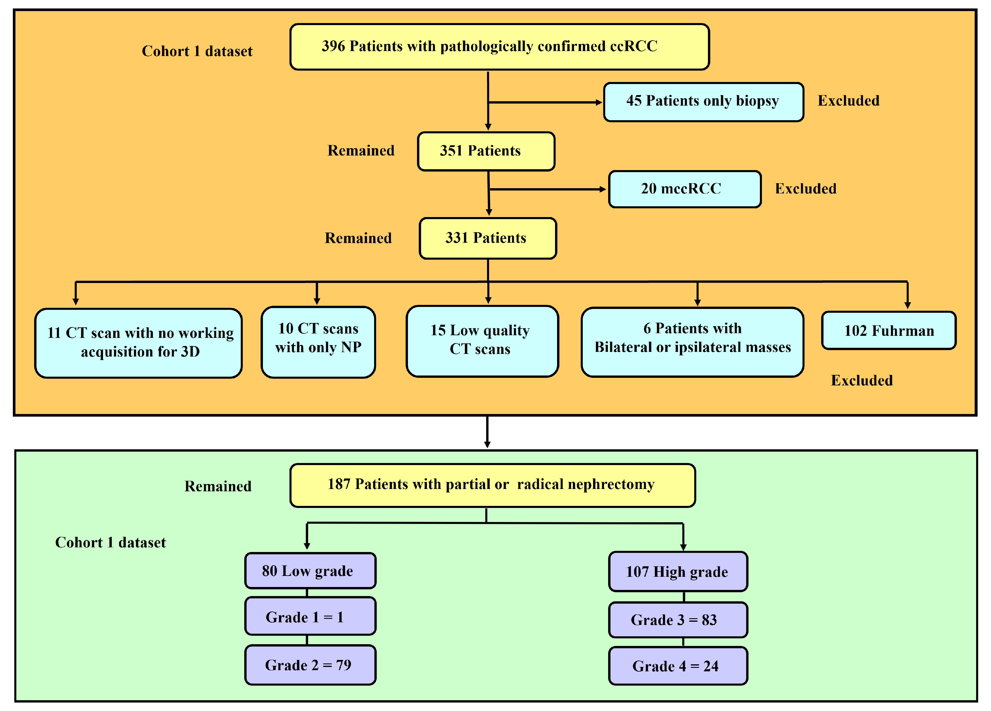
Figure 2.
Manual segmentation of the 3D image slices using Slicer 3D software. (a) Axial plane. (b) Coronal plane. (c) Sagittal plane. (d) Generated 3D VOI from the 2D slices delineated.
Figure 2.
Manual segmentation of the 3D image slices using Slicer 3D software. (a) Axial plane. (b) Coronal plane. (c) Sagittal plane. (d) Generated 3D VOI from the 2D slices delineated.
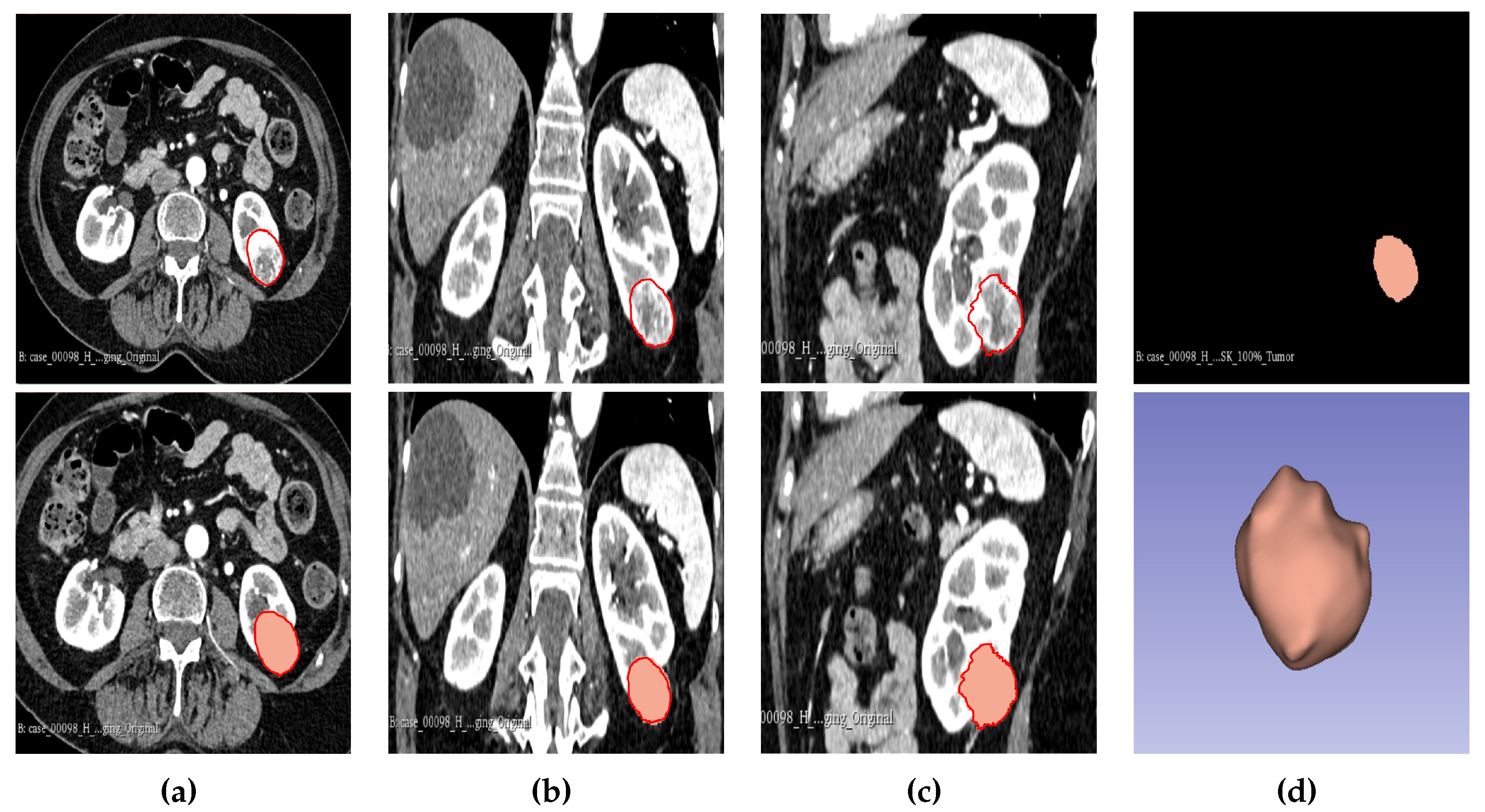
Figure 3.
Manual segmentation of the 3D image slices using Slicer 3D software. (a) 75% periphery and core of the tumour. (b) 50% periphery and core of the tumour. (c) 25% periphery and core of the tumour. (d) Overlap of periphery and core subregions.
Figure 3.
Manual segmentation of the 3D image slices using Slicer 3D software. (a) 75% periphery and core of the tumour. (b) 50% periphery and core of the tumour. (c) 25% periphery and core of the tumour. (d) Overlap of periphery and core subregions.
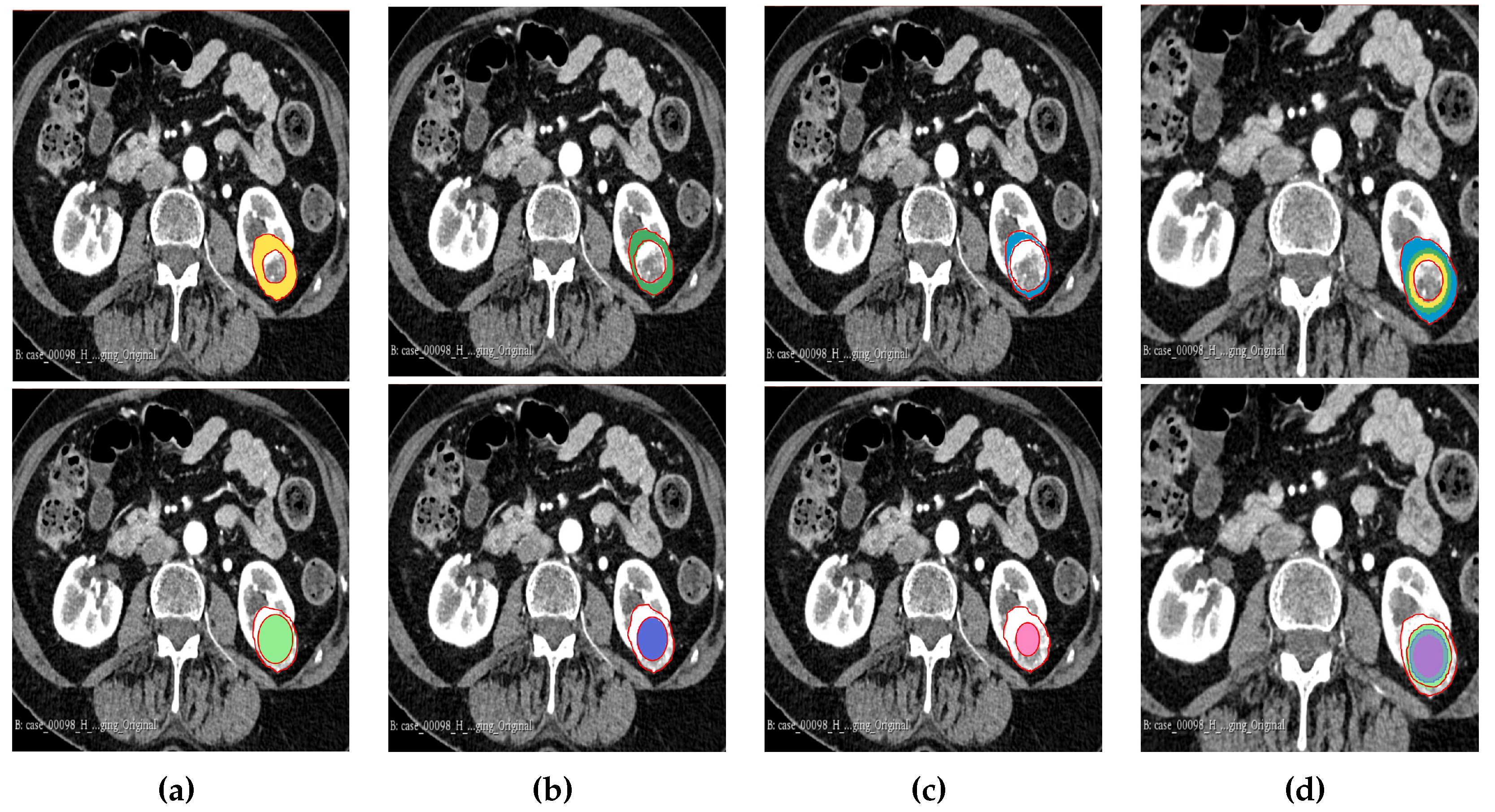
Figure 4.
Representation of the 3D segmented regions. (a) 75% periphery and core of the tumour. (b) 50% periphery and core of the tumour. (c) 25% periphery and core of the tumour. (d) Overlap of periphery and core subregions.
Figure 4.
Representation of the 3D segmented regions. (a) 75% periphery and core of the tumour. (b) 50% periphery and core of the tumour. (c) 25% periphery and core of the tumour. (d) Overlap of periphery and core subregions.
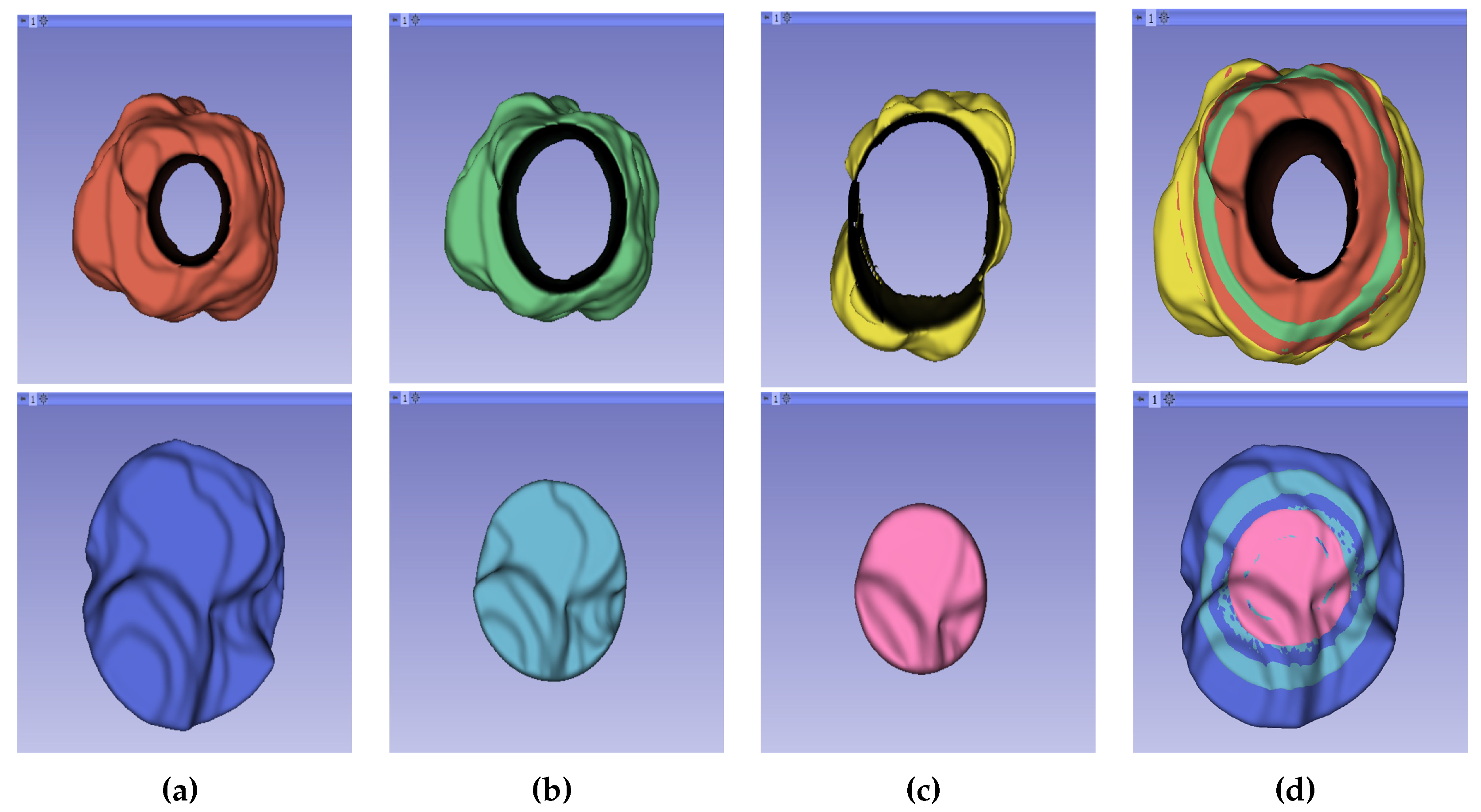
Figure 5.
AUC-ROC curve represents a comparison between biopsy and machine learning.
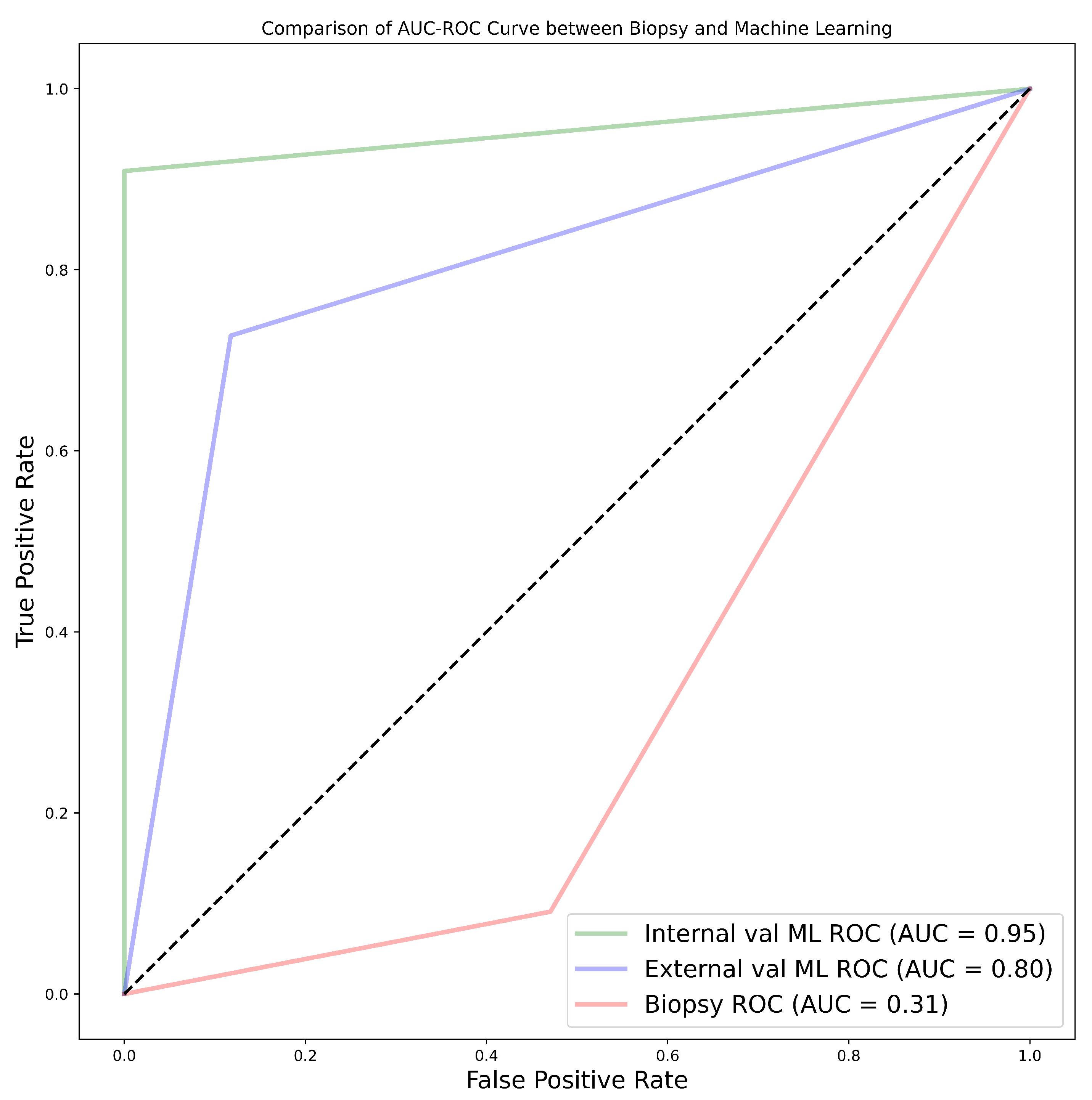

Table 1.
Sample sizes for the different cohorts in the study population.
| TRAINING | TESTING | |||||
|---|---|---|---|---|---|---|
| COHORTS | HIGH | LOW | TOTAL | HIGH | LOW | TOTAL |
| 1 | 76 | 49 | 125 | 31 | 31 | 62 |
| 2 | 56 | 80 | 136 | 21 | 47 | 68 |
| 3 | 122 | 139 | 261 | 62 | 68 | 130 |
| 4 | - | - | - | 11 | 17 | 28 |
Table 2.
Statistical demographic characteristics of the patient’s data.
| Tumours and Patients Characteristics | |||||
|---|---|---|---|---|---|
| Variable | Low Grade | High Grade | p-Value | rpb*1 | |
| Age(Mean ± SD) | 59.05±12.28 | 64±9.40 | 0.002* | 0.4 | |
| Cohort 1 | Size(cm) | 4.32±2.02 | 6.03±3.23 | 0.00006* | 0.6 |
| n=187 | Volume(cm3) | 75.8±90.90 | 203.74±305.82 | 0* | 0.6 |
| Gender | 0.331 | ||||
| Male | 49 (26.20%) | 74 (39.57%) | |||
| Female | 31 (16.58%) | 33 (17.65%) | |||
| Age(Mean ± SD) | 57.17±12.67 | 63.68±11.14 | 0* | 0.88 | |
| Cohort 2 | Size (cm) | 3.89±2.16 | 6.81±3.55 | 0* | 0.45 |
| n=204 | Volume (cm3) | 51.44±114.32 | 235.26±326.10 | 0* | 0.56 |
| Gender | 0.25 | ||||
| Male | 77 (37.75%) | 57 (27.94%) | |||
| Female | 50 (24.51%) | 20 (9.80%) | |||
| Age(Mean ± SD) | 57.89±12.55 | 63.86±10.17 | 0* | 0.56 | |
| Cohort 3 | Size(cm) | 3.89±2.16 | 6.81±3.55 | 0* | 0.2 |
| n=391 | Volume(cm3) | 60.86±106.55 | 216.93±314.85 | 0* | 0.29 |
| Gender | 0.25 | ||||
| Male | 126 (32.23%) | 131 (33.50%) | |||
| Female | 81 (20.72%) | 53 (13.55%) | |||
| Age(Mean ± SD) | 57.12±10.25 | 62.09±9.39 | 0.22 | ||
| Cohort 4 | Size(cm) | 3.31±0.94 | 4.02±2.25 | 0.28 | |
| n=28 | Volume(cm3) | 25.98±27.10 | 57.16±70.40 | 0.13 | |
| Gender | 1 | ||||
| Male | 12 (42.86%) | 8 (28.57%) | |||
| Female | 5 (17.86%) | 3 (10.71%) | |||
| *Statistical significance is at 0.05,*1 point-biserial correlation coefficient (rpb). | |||||
Table 3.
Representation of Cohort 1 diagnostic performance using core subregions and 100% tumour for different models.
Table 3.
Representation of Cohort 1 diagnostic performance using core subregions and 100% tumour for different models.
| COHORT 1 CORE N=187 (107 H, 80 L) | ||||||||||||||
|---|---|---|---|---|---|---|---|---|---|---|---|---|---|---|
| REGION | SVM | RF | XGB | NB | MLP | LSTM | LR | QDA | LGB | CB | ADB | AVG | FS | |
| ACC | 70.97 | 74.19 | 70.97 | 72.58 | 69.35 | 74.19 | 74.19 | 70.97 | 74.19 | 80.65 | 69.35 | 72.87 | ||
| SPE | 70.97 | 70.97 | 70.9 | 67.74 | 70.97 | 80.65 | 70.97 | 67.74 | 70.97 | 80.65 | 74.19 | 72.44 | ||
| SEN | 70.97 | 77.42 | 70.97 | 77.42 | 67.74 | 67.74 | 77.42 | 74.19 | 77.42 | 80.65 | 64.52 | 73.31 | ||
| 75% | AUC | 71±11.3 | 74±10.9 | 71±11.3 | 73±11.1 | 69±11.5 | 74±10.9 | 74±10.9 | 71±11.3 | 74±10.9 | 81±9.8 | 69±11.5 | 72.82 | 7 |
| MCC | 0.42 | 0.48 | 0.42 | 0.45 | 0.39 | 0.49 | 0.48 | 0.42 | 0.48 | 0.61 | 0.39 | - | ||
| F1 | 0.71 | 0.75 | 0.71 | 0.74 | 0.69 | 0.72 | 0.75 | 0.72 | 0.75 | 0.81 | 0.68 | - | ||
| McN | 1.00 | 0.62 | 1.00 | 0.47 | 0.82 | 0.32 | 0.62 | 0.64 | 0.62 | 0.10 | 0.49 | - | ||
| 0.13 | 0.05 | 0.13 | 0.07 | 0.18 | 0.04 | 0.05 | 0.12 | 0.05 | 0 | 0.16 | - | |||
| ACC | 79.03 | 79.03 | 82.26 | 74.19 | 74.19 | 75.81 | 77.42 | 79.03 | 79.03 | 82.26 | 75.81 | 78.01 | ||
| SPE | 74.19 | 74.19 | 87.10 | 70.97 | 74.19 | 77.42 | 74.19 | 74.19 | 70.97 | 77.42 | 70.97 | 73.87 | ||
| SEN | 83.87 | 83.87 | 77.42 | 77.42 | 74.19 | 74.19 | 80.65 | 83.87 | 87.10 | 87.10 | 80.65 | 79.57 | ||
| 50% | AUC | 79±10.1 | 79±10.1 | 82±9.6 | 74±10.9 | 74±10.9 | 76±10.6 | 77±10.5 | 79±10.1 | 79±10.1 | 82±9.6 | 76±10.6 | 77.91 | 8 |
| MCC | 0.58 | 0.58 | 0.65 | 0.48 | 0.48 | 0.52 | 0.55 | 0.58 | 0.59 | 0.65 | 0.52 | - | ||
| F1 | 0.80 | 0.80 | 0.81 | 0.75 | 0.74 | 0.75 | 0.78 | 0.80 | 0.81 | 0.8 | 0.77 | - | ||
| McN | 0.41 | 0.41 | 0.37 | 0.62 | 1.00 | 0.80 | 0.59 | 0.41 | 0.17 | 0.37 | 0.44 | - | ||
| 0.01 | 0.01 | 0 | 0.05 | 0.05 | 0.03 | 0.02 | 0.01 | 0.01 | 0 | 0.03 | - | |||
| ACC | 74.19 | 74.19 | 79.03 | 74.19 | 72.26 | 74.19 | 77.42 | 79.03 | 80.65 | 79.03 | 72.58 | 76.07 | ||
| SPE | 70.97 | 74.19 | 70.97 | 74.19 | 67.74 | 70.97 | 74.19 | 70.97 | 77.42 | 77.42 | 67.74 | 72.43 | ||
| SEN | 77.42 | 74.19 | 87.10 | 74.19 | 77.42 | 77.42 | 80.65 | 87.10 | 83.87 | 80.65 | 77.42 | 78.14 | ||
| 25% | AUC | 74±10.9 | 74±10.9 | 79±10.1 | 74±10.9 | 73±11.1 | 74±10.9 | 77±10.5 | 79±10.1 | 81±9.8 | 79±10.1 | 73±11.1 | 76.09 | 19 |
| MCC | 0.48 | 0.48 | 0.59 | 0.48 | 0.45 | 0.48 | 0.55 | 0.59 | 0.61 | 0.58 | 0.45 | - | ||
| F1 | 0.75 | 0.74 | 0.81 | 0.74 | 0.74 | 0.75 | 0.78 | 0.81 | 0.81 | 0.79 | 0.74 | - | ||
| McN | 0.62 | 1.00 | 0.17 | 1.00 | 0.47 | 0.62 | 0.59 | 0.17 | 0.56 | 0.78 | 0.47 | - | ||
| 0.05 | 0.05 | 0.01 | 0.05 | 0.07 | 0.05 | 0.02 | 0.01 | 0.00 | 0.01 | 0.07 | - | |||
| AVG | AUC | 74.67 | 75.67 | 77.33 | 73.67 | 72.00 | 74.67 | 76.00 | 76.33 | 78.00 | 80.67 | 72.67 | - | |
| ACC | 77.42 | 79.03 | 79.03 | 74.19 | 69.35 | 72.00 | 75.81 | 75.81 | 74.19 | 85.48 | 77.42 | 76.33 | ||
| SPE | 77.42 | 70.97 | 77.42 | 70.97 | 70.97 | 70.97 | 74.19 | 74.19 | 77.42 | 77.42 | 74.19 | 74.19 | ||
| SEN | 77.42 | 87.10 | 80.65 | 77.420 | 67.74 | 74.19 | 77.42 | 77.42 | 70.97 | 93.55 | 80.65 | 78.59 | ||
| 100% | AUC | 77±10.5 | 79±10.1 | 79±10.1 | 74±10.9 | 69±11.5 | 73±11.1 | 76±10.6 | 76±10.6 | 74±10.9 | 85±8.9 | 77±10.5 | 76.27 | 16 |
| MCC | 0.55 | 0.59 | 0.58 | 0.48 | 0.39 | 0.45 | 0.52 | 0.52 | 0.48 | 0.72 | 0.55 | - | ||
| F1 | 0.77 | 0.81 | 0.79 | 0.75 | 0.69 | 0.73 | 0.76 | 0.76 | 0.73 | 0.87 | 0.78 | - | ||
| McN | 1.00 | 0.17 | 0.78 | 0.62 | 0.82 | 0.81 | 0.80 | 0.80 | 0.62 | 0.10 | 0.59 | - | ||
| 0.02 | 0.01 | 0.01 | 0.05 | 0.18 | 0.08 | 0.03 | 0.03 | 0.05 | 0 | 0.02 | - | |||
Table 4.
Representation of cohort 1 diagnostic performance using periphery subregions for different models.
Table 4.
Representation of cohort 1 diagnostic performance using periphery subregions for different models.
| COHORT 1 PERIPHERY N=187 (107 H, 80 L) | ||||||||||||||
|---|---|---|---|---|---|---|---|---|---|---|---|---|---|---|
| REGION | SVM | RF | XGB | NB | MLP | LSTM | LR | QDA | LGB | CB | ADB | AVG | FS | |
| ACC | 74.19 | 74.19 | 70.97 | 75.81 | 70.97 | 69.00 | 70.97 | 74.19 | 70.97 | 77.42 | 72.58 | 72.84 | ||
| SPE | 70.97 | 70.97 | 70.97 | 80.65 | 70.97 | 77.42 | 67.74 | 67.74 | 70.97 | 77.42 | 70.97 | 72.44 | ||
| SEN | 77.42 | 77.42 | 70.97 | 70.97 | 70.97 | 61.29 | 74.19 | 80.65 | 70.97 | 77.42 | 74.19 | 73.31 | ||
| 75% | AUC | 74±10.9 | 74±10.9 | 71±11.3 | 76±10.6 | 71±11.3 | 69±11.5 | 71±11.3 | 74±10.9 | 71±11.3 | 77±10.5 | 73±11.1 | 72.82 | 8 |
| MCC | 0.48 | 0.48 | 0.42 | 0.52 | 0.42 | 0.39 | 0.42 | 0.49 | 0.42 | 0.55 | 0.45 | - | ||
| F1 | 0.75 | 0.75 | 0.71 | 0.75 | 0.71 | 0.67 | 0.72 | 0.76 | 0.71 | 0.77 | 0.73 | - | ||
| McN | 0.62 | 0.62 | 1.00 | 0.44 | 1.00 | 0.25 | 0.64 | 0.32 | 1.00 | 1.00 | 0.81 | - | ||
| 0.05 | 0.05 | 0.13 | 0.03 | 0.13 | 0.12 | 0.12 | 0.04 | 0.13 | 0.02 | 0.08 | - | |||
| ACC | 70.97 | 75.81 | 79.03 | 72.58 | 72.58 | 69.35 | 74.19 | 74.19 | 74.19 | 77.42 | 70.97 | 73.75 | ||
| SPE | 70.97 | 74.19 | 70.97 | 70.97 | 70.97 | 64.52 | 74.19 | 64.52 | 61.29 | 77.42 | 64.52 | 69.50 | ||
| SEN | 70.97 | 77.42 | 87.10 | 74.19 | 74.19 | 74.19 | 74.19 | 83.87 | 87.10 | 77.42 | 77.42 | 75.98 | ||
| 50% | AUC | 71±11.3 | 76±10.6 | 79±10.1 | 73±11.1 | 73±11.1 | 69±11.5 | 74±10.9 | 74±10.9 | 74±10.9 | 77±10.5 | 71±11.3 | 73.73 | 11 |
| MCC | 0.42 | 0.52 | 0.59 | 0.45 | 0.45 | 0.39 | 0.48 | 0.49 | 0.50 | 0.55 | 0.42 | - | ||
| F1 | 0.71 | 0.76 | 0.81 | 0.73 | 0.73 | 0.71 | 0.74 | 0.76 | 0.77 | 0.77 | 0.72 | - | ||
| McN | 1.00 | 0.80 | 0.17 | 0.81 | 0.81 | 0.49 | 1.00 | 0.13 | 0.05 | 1.00 | 0.35 | - | ||
| 0.13 | 0.03 | 0.01 | 0.08 | 0.08 | 0.16 | 0.05 | 0.02 | 0.01 | 0.02 | 0.09 | - | |||
| ACC | 77.42 | 80.65 | 79.03 | 82.26 | 75.81 | 72.58 | 77.42 | 80.65 | 79.03 | 83.87 | 75.81 | 78.59 | ||
| SPE | 74.19 | 80.65 | 70.97 | 83.87 | 80.65 | 70.97 | 77.42 | 74.19 | 74.19 | 80.65 | 64.52 | 75.66 | ||
| SEN | 80.65 | 89.65 | 87.10 | 80.65 | 77.42 | 74.19 | 77.42 | 87.10 | 83.87 | 87.10 | 87.1 | 81.37 | ||
| 25% | AUC | 77±10.5 | 81±9.8 | 79±10.1 | 82±9.6 | 76±10.6 | 73±11.1 | 77±10.5 | 81±9.8 | 79±10.1 | 84±9.1 | 76±10.6 | 78.64 | 9 |
| MCC | 0.55 | 0.61 | 0.59 | 0.65 | 0.52 | 0.45 | 0.55 | 0.62 | 0.58 | 0.68 | 0.53 | - | ||
| F1 | 0.78 | 0.81 | 0.81 | 0.82 | 0.77 | 0.73 | 0.77 | 0.82 | 0.80 | 0.84 | 0.78 | - | ||
| McN | 0.59 | 1.00 | 0.17 | 0.76 | 0.44 | 0.81 | 1.00 | 0.25 | 0.41 | 0.53 | 0.07 | - | ||
| 0.02 | 0 | 0.01 | 0 | 0.03 | 0.08 | 0.02 | 0.00 | 0.01 | 0 | 0.01 | - | |||
| AVG | AUC | 74.00 | 77.00 | 76.33 | 77.00 | 73.33 | 70.33 | 74.00 | 76.33 | 78.00 | 79.33 | 73.33 | - | |
Table 5.
Representation of cohort 2 diagnostic performance using core subregions and 100% tumour for different models.
Table 5.
Representation of cohort 2 diagnostic performance using core subregions and 100% tumour for different models.
| COHORT 2 CORE N=204 (77 H, 127 L) | ||||||||||||||
|---|---|---|---|---|---|---|---|---|---|---|---|---|---|---|
| REGION | SVM | RF | XGB | NB | MLP | LSTM | LR | QDA | LGB | CB | ADB | AVG | FS | |
| ACC | 86.79 | 85.29 | 82.35 | 80.88 | 82.00 | 82.30 | 85.29 | 85.29 | 80.88 | 86.76 | 77.94 | 83.50 | ||
| SPE | 93.62 | 85.11 | 78.72 | 80.85 | 82.98 | 83.00 | 89.36 | 89.36 | 76.60 | 87.23 | 76.6 | 84.87 | ||
| SEN | 71.43 | 85.71 | 90.48 | 80.95 | 80.95 | 80.95 | 76.19 | 76.19 | 90.48 | 85.71 | 80.95 | 81.82 | ||
| 75% | AUC | 83±8.9 | 85±8.5 | 85±8.5 | 81±9.3 | 82±9.1 | 82±9.1 | 83±8.9 | 83±8.9 | 84±8.7 | 86±8.2 | 79±9.7 | 83 | 9 |
| MCC | 0.68 | 0.68 | 0.65 | 0.59 | 0.61 | 0.61 | 0.66 | 0.66 | 0.62 | 0.71 | 0.54 | - | ||
| F1 | 0.77 | 0.78 | 0.76 | 0.72 | 0.74 | 0.74 | 0.76 | 0.76 | 0.75 | 0.80 | 0.69 | - | ||
| McN | 0.32 | 0.21 | 0.02 | 0.17 | 0.25 | 0.25 | 1.00 | 1.00 | 0.01 | 0.32 | 0.07 | - | ||
| 0 | 0 | 0 | 0 | 0 | 0 | 0 | 0 | 0 | 0 | 0 | - | |||
| ACC | 88.24 | 88.24 | 89.71 | 88.24 | 85.00 | 83.82 | 88.24 | 91.18 | 88.24 | 89.71 | 86.76 | 87.94 | ||
| SPE | 91.49 | 87.23 | 87.23 | 91.49 | 85.11 | 80.85 | 95.75 | 91.49 | 85.11 | 89.36 | 85.11 | 88.20 | ||
| SEN | 80.95 | 90.48 | 90.48 | 89.95 | 85.71 | 90.48 | 71.43 | 90.48 | 95.24 | 90.48 | 90.48 | 87.83 | ||
| 50% | AUC | 86±8.2 | 89±7.4 | 89±7.4 | 86±8.2 | 85±8.5 | 86±8.2 | 84±8.7 | 91±6.8 | 90±7.1 | 90±7.1 | 88±7.7 | 87.64 | 12 |
| MCC | 0.72 | 0.74 | 0.74 | 0.72 | 0.68 | 0.67 | 0.72 | 0.80 | 0.76 | 0.77 | 0.72 | - | ||
| F1 | 0.81 | 0.83 | 0.83 | 0.81 | 0.78 | 0.78 | 0.79 | 0.86 | 0.83 | 0.84 | 0.81 | - | ||
| McN | 1.00 | 0.16 | 0.16 | 1.00 | 0.21 | 0.03 | 0.16 | 0.41 | 0.03 | 0.26 | 0.1 | - | ||
| 0 | 0 | 0 | 0 | 0 | 0 | 0 | 0 | 0 | 0 | 0 | - | |||
| ACC | 85.29 | 85.29 | 82.35 | 82.35 | 79.00 | 79.41 | 82.35 | 83.82 | 80.00 | 85.29 | 85.29 | 83.49 | ||
| SPE | 85.12 | 85.11 | 80.85 | 82.98 | 78.72 | 80.85 | 82.98 | 82.98 | 80.85 | 85.11 | 87.23 | 82.98 | ||
| SEN | 85.71 | 85.71 | 85.71 | 80.95 | 80.95 | 76.19 | 80.95 | 85.71 | 80.95 | 85.71 | 80.95 | 82.68 | ||
| 25% | AUC | 85±8.5 | 85±8.5 | 83±8.9 | 82±9.1 | 80±9.5 | 79±9.7 | 82±9.1 | 84±8.7 | 81±9.3 | 85±8.5 | 84±8.7 | 82.73 | 10 |
| MCC | 0.68 | 0.68 | 0.63 | 0.61 | 0.56 | 0.55 | 0.61 | 0.65 | 0.59 | 0.68 | 0.67 | - | ||
| F1 | 0.78 | 0.78 | 0.75 | 0.74 | 0.71 | 0.70 | 0.74 | 0.77 | 0.72 | 0.78 | 0.77 | - | ||
| McN | 0.21 | 0.21 | 0.08 | 0.25 | 0.11 | 0.29 | 0.25 | 0.13 | 0.17 | 0.21 | 0.53 | - | ||
| 0 | 0 | 0 | 0 | 0 | 0 | 0 | 0 | 0 | 0 | 0 | - | |||
| AVG | AUC | 84.67 | 86.33 | 85.67 | 83.00 | 82.33 | 82.33 | 83.00 | 86.00 | 85.00 | 87.00 | 83.67 | - | |
| ACC | 85.29 | 85.29 | 80.88 | 85.29 | 82.00 | 82.35 | 82.35 | 82.35 | 86.76 | 86.76 | 83.82 | 84.11 | ||
| SPE | 91.49 | 85.11 | 82.98 | 87.23 | 82.98 | 85.11 | 80.85 | 80.85 | 89.36 | 87.23 | 85.11 | 85.30 | ||
| SEN | 71.43 | 85.71 | 76.19 | 80.95 | 80.95 | 76.19 | 85.71 | 85.71 | 80.95 | 85.71 | 80.95 | 80.95 | ||
| 100% | AUC | 81±9.3 | 85±8.5 | 80±9.5 | 84±8.7 | 82±9.1 | 81±9.3 | 83±8.9 | 83±8.9 | 85±8.5 | 86±8.2 | 83±8.9 | 83 | 9 |
| MCC | 0.65 | 0.68 | 0.57 | 0.67 | 0.61 | 0.60 | 0.63 | 0.63 | 0.69 | 0.71 | 0.64 | - | ||
| F1 | 0.75 | 0.78 | 0.71 | 0.77 | 0.74 | 0.73 | 0.75 | 0.75 | 0.79 | 0.80 | 0.76 | - | ||
| McN | 0.53 | 0.21 | 0.41 | 0.53 | 0.25 | 0.56 | 0.08 | 0.08 | 0.74 | 0.32 | 0.37 | - | ||
| 0 | 0 | 0 | 0 | 0 | 0 | 0 | 0 | 0 | 0 | 0 | - | |||
Table 6.
Representation of cohort 2 diagnostic performance using periphery subregions for different models
Table 6.
Representation of cohort 2 diagnostic performance using periphery subregions for different models
| COHORT 2 PERIPHERY N=204 (77 H, 127 L) | ||||||||||||||
|---|---|---|---|---|---|---|---|---|---|---|---|---|---|---|
| REGION | SVM | RF | XGB | NB | MLP | LSTM | LR | QDA | LGB | CB | ADB | AVG | FS | |
| ACC | 88.24 | 85.29 | 83.82 | 86.76 | 79.40 | 76.47 | 76.47 | 86.76 | 80.88 | 85.29 | 88.24 | 83.82 | ||
| SPE | 95.75 | 82.36 | 85.12 | 91.49 | 76.60 | 72.34 | 89.36 | 93.62 | 80.85 | 87.23 | 87.23 | 86.81 | ||
| SEN | 71.43 | 85.71 | 80.95 | 76.19 | 85.71 | 85.71 | 71.43 | 71.43 | 80.95 | 80.95 | 76.19 | 78.79 | ||
| 75% | AUC | 84±8.7 | 85±8.5 | 83±8.9 | 84±8.7 | 81±9.3 | 79±9.7 | 80±9.5 | 83±8.9 | 81±9.3 | 84±8.7 | 82±9.1 | 82.36 | 8 |
| MCC | 0.72 | 0.68 | 0.64 | 0.69 | 0.58 | 0.54 | 0.62 | 0.68 | 0.59 | 0.67 | 0.63 | - | ||
| F1 | 0.79 | 0.78 | 0.76 | 0.78 | 0.72 | 0.69 | 0.73 | 0.77 | 0.72 | 0.77 | 0.74 | - | ||
| McN | 0.16 | 0.21 | 0.37 | 0.74 | 0.03 | 0.01 | 0.76 | 0.32 | 0.17 | 0.53 | 0.76 | - | ||
| 0 | 0 | 0 | 0 | 0 | 0 | 0 | 0 | 0 | 0 | 0 | - | |||
| ACC | 86.76 | 88.24 | 75.00 | 85.29 | 75.00 | 79.40 | 76.47 | 88.24 | 76.47 | 91.18 | 88.24 | 85.11 | ||
| SPE | 91.49 | 95.75 | 70.21 | 87.23 | 70.21 | 78.72 | 76.60 | 95.75 | 72.34 | 91.49 | 95.75 | 84.89 | ||
| SEN | 76.19 | 71.43 | 85.71 | 80.95 | 85.71 | 80.95 | 76.19 | 71.43 | 85.71 | 90.48 | 71.43 | 79.65 | ||
| 50% | AUC | 84±8.7 | 84±8.7 | 78±9.8 | 84±8.7 | 78±9.8 | 80±9.5 | 76±10.2 | 84±8.7 | 79±9.7 | 91±6.8 | 84±8.7 | 82 | 12 |
| MCC | 0.69 | 0.72 | 0.52 | 0.67 | 0.52 | 0.56 | 0.50 | 0.72 | 0.54 | 0.80 | 0.72 | - | ||
| F1 | 0.78 | 0.79 | 0.68 | 0.77 | 0.68 | 0.71 | 0.67 | 0.79 | 0.69 | 0.86 | 0.79 | - | ||
| McN | 0.74 | 0.16 | 0.01 | 0.53 | 0.01 | 0.11 | 0.13 | 0.16 | 0.01 | 0.41 | 0.16 | - | ||
| 0 | 0 | 0 | 0 | 0 | 0 | 0 | 0 | 0 | 0 | 0 | - | |||
| ACC | 85.29 | 85.29 | 76.47 | 82.35 | 77.94 | 75.00 | 76.47 | 89.71 | 80.88 | 83.82 | 85.29 | 82.351 | ||
| SPE | 85.12 | 87.23 | 72.34 | 82.98 | 76.60 | 74.47 | 78.72 | 93.62 | 82.98 | 85.11 | 85.11 | 82.77 | ||
| SEN | 85.71 | 80.95 | 85.71 | 80.95 | 80.95 | 76.19 | 71.43 | 80.95 | 76.19 | 80.95 | 85.71 | 80.52 | ||
| 25% | AUC | 85±8.5 | 84±8.7 | 79±9.7 | 82±9.1 | 79±9.7 | 75±10.3 | 75±10.3 | 87±8 | 80±9.5 | 83±8.9 | 85±8.5 | 81.27 | 16 |
| MCC | 0.68 | 0.67 | 0.54 | 0.61 | 0.54 | 0.48 | 0.48 | 0.76 | 0.57 | 0.64 | 0.68 | - | ||
| F1 | 0.78 | 0.77 | 0.69 | 0.74 | 0.69 | 0.65 | 0.65 | 0.83 | 0.71 | 0.76 | 0.78 | - | ||
| McN | 0.21 | 0.53 | 0.01 | 0.25 | 0.07 | 0.09 | 0.32 | 0.71 | 0.41 | 0.37 | 0.21 | - | ||
| 0 | 0 | 0 | 0 | 0 | 0 | 0 | 0 | 0 | 0 | 0 | - | |||
| AVG | AUC | 84.33 | 84.33 | 80.00 | 83.33 | 79.33 | 78.00 | 77.00 | 84.67 | 80.00 | 86.00 | 83.67 | - | |
Table 7.
Representation of cohort 3 diagnostic performance using core subregions and 100% tumour for different models.
Table 7.
Representation of cohort 3 diagnostic performance using core subregions and 100% tumour for different models.
| COHORT 3 CORE N=391 (184 H, 207 L) | ||||||||||||||
|---|---|---|---|---|---|---|---|---|---|---|---|---|---|---|
| REGION | SVM | RF | XGB | NB | MLP | LSTM | LR | QDA | LGB | CB | ADB | AVG | FS | |
| ACC | 70.77 | 76.92 | 74.62 | 71.54 | 73.08 | 71.54 | 73.08 | 74.62 | 73.08 | 76.15 | 73.85 | 73.57 | ||
| SPE | 69.12 | 76.47 | 73.53 | 73.53 | 77.94 | 72.06 | 70.59 | 77.94 | 76.47 | 77.94 | 76.47 | 74.73 | ||
| SEN | 72.58 | 77.42 | 75.81 | 69.36 | 67.74 | 70.97 | 75.81 | 70.97 | 69.35 | 74.19 | 70.97 | 72.29 | ||
| 75% | AUC | 71±7.8 | 77±7.2 | 75±7.4 | 71±7.8 | 73±7.6 | 72±7.7 | 73±7.6 | 74±7.5 | 73±7.6 | 76±7.3 | 74±7.5 | 73.55 | 14 |
| MCC | 0.42 | 0.54 | 0.49 | 0.43 | 0.46 | 0.43 | 0.46 | 0.49 | 0.46 | 0.52 | 0.48 | - | ||
| F1 | 0.70 | 0.76 | 0.74 | 0.70 | 0.71 | 0.70 | 0.73 | 0.73 | 0.71 | 0.75 | 0.72 | - | ||
| McN | 0.52 | 0.72 | 0.60 | 0.87 | 0.40 | 0.87 | 0.40 | 0.60 | 0.61 | 0.86 | 0.73 | - | ||
| 0.01 | 0 | 0 | 0 | 0 | 0.01 | 0 | 0 | 0 | 0 | 0 | - | |||
| ACC | 76.92 | 76.92 | 76.15 | 76.92 | 73.08 | 76.15 | 77.69 | 79.23 | 78.46 | 80.00 | 74.62 | 76.614 | ||
| SPE | 75.00 | 77.94 | 77.94 | 77.94 | 70.59 | 72.06 | 76.47 | 76.47 | 77.94 | 79.41 | 76.47 | 76.323 | ||
| SEN | 79.03 | 75.81 | 74.19 | 75.81 | 75.81 | 80.65 | 79.03 | 82.26 | 79.03 | 80.65 | 72.58 | 77.71 | ||
| 50% | AUC | 77±7.2 | 77±7.2 | 76±7.3 | 77±7.2 | 73±7.6 | 76±7.3 | 78±7.1 | 79±7 | 78±7.1 | 80±6.9 | 75±7.4 | 76.91 | 24 |
| MCC | 0.54 | 0.54 | 0.52 | 0.54 | 0.46 | 0.53 | 0.55 | 0.59 | 0.57 | 0.60 | 0.49 | - | ||
| F1 | 0.77 | 0.76 | 0.75 | 0.76 | 0.73 | 0.76 | 0.77 | 0.79 | 0.78 | 0.79 | 0.73 | - | ||
| McN | 0.47 | 1.00 | 0.86 | 1.00 | 0.40 | 0.21 | 0.58 | 0.34 | 0.71 | 0.69 | 0.86 | - | ||
| 0 | 0 | 0 | 0 | 0 | 0 | 0 | 0 | 0 | 0 | 0 | - | |||
| ACC | 74.62 | 74.62 | 72.13 | 73.08 | 72.31 | 71.54 | 71.54 | 73.08 | 73.08 | 76.15 | 70.77 | 72.99 | ||
| SPE | 80.88 | 75.00 | 75.00 | 72.06 | 76.47 | 72.06 | 70.59 | 72.06 | 73.53 | 77.94 | 72.06 | 74.18 | ||
| SEN | 67.74 | 74.19 | 69.36 | 74.19 | 67.74 | 70.97 | 72.58 | 74.19 | 72.58 | 74.19 | 69.36 | 71.55 | ||
| 25% | AUC | 74±7.5 | 75±7.4 | 72±7.7 | 73±7.6 | 72±7.7 | 72±7.7 | 72±7.7 | 73±7.6 | 73±7.6 | 76±7.3 | 71±7.8 | 73 | 32 |
| MCC | 0.49 | 0.49 | 0.44 | 0.46 | 0.44 | 0.43 | 0.43 | 0.46 | 0.46 | 0.52 | 0.41 | 0.46 | ||
| F1 | 0.72 | 0.74 | 0.70 | 0.73 | 0.70 | 0.70 | 0.71 | 0.72 | 0.72 | 0.75 | 0.69 | - | ||
| McN | 0.22 | 0.86 | 0.74 | 0.61 | 0.50 | 0.87 | 0.62 | 0.61 | 0.87 | 0.86 | 1.00 | - | ||
| 0 | 0 | 0 | 0 | 0 | 0.01 | 0.01 | 0 | 0 | 0 | 0.01 | - | |||
| AVG | AUC | 74.00 | 76.33 | 74.33 | 73.67 | 72.67 | 73.33 | 74.33 | 75.33 | 74.67 | 77.33 | 73.33 | - | |
| ACC | 73.85 | 76.15 | 75.38 | 75.38 | 71.54 | 73.85 | 74.62 | 75.38 | 78.46 | 78.46 | 74.62 | 75.24 | ||
| SPE | 73.53 | 72.06 | 77.94 | 79.41 | 76.47 | 72.06 | 70.59 | 76.47 | 82.35 | 80.88 | 76.47 | 76.20 | ||
| SEN | 74.19 | 80.65 | 72.58 | 70.97 | 66.13 | 75.81 | 79.03 | 74.19 | 74.19 | 75.81 | 72.58 | 74.19 | ||
| 100% | AUC | 74±7.5 | 76±7.3 | 75±7.4 | 75±7.4 | 71±7.8 | 74±7.5 | 75±7.4 | 75±7.4 | 78±7.1 | 78±7.1 | 75±7.4 | 75.09 | 15 |
| MCC | 0.48 | 0.53 | 0.51 | 0.51 | 0.43 | 0.48 | 0.50 | 0.51 | 0.57 | 0.57 | 0.49 | - | ||
| F1 | 0.73 | 0.76 | 0.74 | 0.73 | 0.69 | 0.73 | 0.75 | 0.74 | 0.77 | 0.77 | 0.73 | - | ||
| McN | 0.73 | 0.21 | 0.72 | 0.48 | 0.41 | 0.49 | 0.22 | 1.00 | 0.45 | 0.71 | 0.86 | - | ||
| 0 | 0 | 0 | 0 | 0 | 0 | 0 | 0 | 0 | 0 | 0 | - | |||
Table 8.
Representation of cohort 3 diagnostic performance using periphery subregions for different models.
Table 8.
Representation of cohort 3 diagnostic performance using periphery subregions for different models.
| COHORT 3 PERIPHERY N=391 (184 H, 207 L) | ||||||||||||||
|---|---|---|---|---|---|---|---|---|---|---|---|---|---|---|
| REGION | SVM | RF | XGB | NB | MLP | LSTM | LR | QDA | LGB | CB | ADB | AVG | FS | |
| ACC | 70.00 | 80.00 | 74.62 | 71.54 | 70.00 | 70.77 | 72.31 | 75.38 | 73.08 | 77.69 | 72.31 | 73.46 | ||
| SPE | 70.59 | 82.35 | 73.53 | 72.06 | 70.56 | 69.12 | 70.59 | 77.94 | 76.47 | 77.94 | 72.06 | 73.93 | ||
| SEN | 69.36 | 77.42 | 75.81 | 70.97 | 69.36 | 72.58 | 74.19 | 72.58 | 69.36 | 77.42 | 72.58 | 72.88 | ||
| 75% | AUC | 70±7.9 | 80±6.9 | 75±7.4 | 72±7.7 | 70±7.9 | 71±7.8 | 72±7.7 | 75±7.4 | 73±7.6 | 78±7.1 | 72±7.7 | 73.45 | 22 |
| MCC | 0.40 | 0.60 | 0.49 | 0.43 | 0.40 | 0.42 | 0.45 | 0.51 | 0.46 | 0.55 | 0.45 | - | ||
| F1 | 0.69 | 0.79 | 0.74 | 0.70 | 0.69 | 0.70 | 0.72 | 0.74 | 0.71 | 0.77 | 0.71 | - | ||
| McN | 0.87 | 0.69 | 0.60 | 0.87 | 0.87 | 0.52 | 0.50 | 0.72 | 0.61 | 0.85 | 0.74 | - | ||
| 0.01 | 0 | 0 | 0.01 | 0.01 | 0.01 | 0 | 0 | 0 | 0 | 0 | - | |||
| ACC | 73.85 | 76.92 | 75.38 | 72.31 | 70.00 | 71.54 | 75.38 | 74.62 | 74.62 | 76.15 | 69.23 | 74.00 | ||
| SPE | 70.59 | 77.94 | 75.00 | 72.06 | 75.00 | 69.12 | 69.12 | 80.88 | 69.12 | 70.59 | 66.18 | 71.73 | ||
| SEN | 77.42 | 75.81 | 75.81 | 72.58 | 64.52 | 74.19 | 82.26 | 67.74 | 80.65 | 82.26 | 72.58 | 75.07 | ||
| 50% | AUC | 74±7.5 | 77±7.2 | 75±7.4 | 72±7.7 | 70±7.9 | 72±7.7 | 76±7.3 | 74±7.5 | 75±7.4 | 76±7.3 | 69±8 | 73.64 | 26 |
| McC | 0.48 | 0.54 | 0.51 | 0.45 | 0.40 | 0.43 | 0.52 | 0.49 | 0.50 | 0.53 | 0.39 | - | ||
| F1 | 0.74 | 0.76 | 0.75 | 0.71 | 0.67 | 0.71 | 0.76 | 0.72 | 0.75 | 0.77 | 0.69 | - | ||
| McN | 0.30 | 1.00 | 0.72 | 0.74 | 0.42 | 0.41 | 0.08 | 0.22 | 0.12 | 0.11 | 0.34 | - | ||
| 0 | 0 | 0 | 0 | 0.01 | 0 | 0 | 0 | 0 | 0 | 0.01 | - | |||
| ACC | 75.38 | 77.69 | 76.92 | 75.38 | 73.08 | 73.08 | 75.38 | 75.38 | 76.15 | 76.15 | 74.62 | 75.38 | ||
| SPE | 83.82 | 77.94 | 80.88 | 76.47 | 72.06 | 73.53 | 76.47 | 72.06 | 77.94 | 73.53 | 75.00 | 76.47 | ||
| SEN | 66.13 | 77.42 | 72.58 | 74.19 | 74.19 | 72.58 | 74.19 | 79.03 | 74.19 | 79.03 | 74.19 | 74.34 | ||
| 25% | AUC | 75±7.4 | 78±7.1 | 77±7.2 | 75±7.4 | 73±7.6 | 73±7.6 | 75±7.4 | 76±7.3 | 76±7.3 | 76±7.3 | 75±7.4 | 75.36 | 21 |
| MCC | 0.51 | 0.55 | 0.54 | 0.51 | 0.46 | 0.46 | 0.51 | 0.51 | 0.52 | 0.53 | 0.49 | - | ||
| F1 | 0.72 | 0.77 | 0.75 | 0.74 | 0.72 | 0.72 | 0.74 | 0.75 | 0.75 | 0.76 | 0.74 | - | ||
| McN | 0.08 | 0.85 | 0.47 | 1.00 | 0.61 | 0.87 | 1.00 | 0.29 | 0.86 | 0.37 | 0.86 | - | ||
| 0 | 0 | 0 | 0 | 0 | 0 | 0 | 0 | 0 | 0 | 0 | - | |||
| AVG | AUC | 73.00 | 78.33 | 75.67 | 73.00 | 71.00 | 72.00 | 74.33 | 75.00 | 74.67 | 76.67 | 72.00 | - | |
Table 9.
Representation of the diagnostic performance for the external validation of cohort 1 using cores subregions for different models.
Table 9.
Representation of the diagnostic performance for the external validation of cohort 1 using cores subregions for different models.
| COHORT 1 CORE EXTERNAL VALIDATION | ||||||||||||||
|---|---|---|---|---|---|---|---|---|---|---|---|---|---|---|
| REGION | SVM | RF | XGB | NB | MLP | LSTM | LR | QDA | LGB | CB | ADB | AVG | FS | |
| ACC | 66.31 | 64.71 | 64.71 | 62.03 | 60.96 | 63.1 | 64.71 | 66.31 | 62.03 | 65.78 | 62.57 | 63.93 | ||
| SPE | 61.25 | 47.50 | 55.00 | 55.00 | 53.75 | 53.75 | 63.75 | 68.75 | 47.5 | 58.75 | 45.00 | 56.25 | ||
| SEN | 70.09 | 77.57 | 71.96 | 67.29 | 66.36 | 70.09 | 65.42 | 64.49 | 72.90 | 71.03 | 75.70 | 70.26 | ||
| 75% | AUC | 66±6.8 | 63±6.9 | 63±6.9 | 61±7 | 60±7 | 62±7 | 65±6.8 | 67±6.7 | 60±7 | 65±6.8 | 60±7 | 62.91 | 19 |
| MCC | 0.31 | 0.26 | 0.27 | 0.22 | 0.20 | 0.24 | 0.29 | 0.33 | 0.21 | 0.30 | 0.22 | - | ||
| F1 | 0.7 | 0.72 | 0.70 | 0.67 | 0.66 | 0.68 | 0.68 | 0.69 | 0.69 | 0.70 | 0.70 | - | ||
| McN | 0.90 | 0.03 | 0.46 | 0.91 | 0.91 | 0.55 | 0.32 | 0.10 | 0.12 | 0.80 | 0.03 | - | ||
| 0.01 | 0 | 0.01 | 0.04 | 0.05 | 0.01 | 0.02 | 0.01 | 0 | 0.01 | 0 | - | |||
| ACC | 68.45 | 64.71 | 62.57 | 63.1 | 60.96 | 62.57 | 68.45 | 70.05 | 64.71 | 68.45 | 63.10 | 65.19 | ||
| SPE | 57.50 | 57.50 | 58.75 | 63.75 | 51.25 | 63.75 | 62.50 | 62.50 | 55.00 | 60.00 | 47.50 | 58.18 | ||
| SEN | 76.64 | 70.09 | 65.42 | 62.62 | 68.22 | 61.68 | 72.90 | 75.70 | 71.96 | 74.77 | 74.77 | 70.43 | ||
| 50% | AUC | 67±6.7 | 64±6.9 | 62±7 | 63±6.9 | 60±7 | 63±6.9 | 68±6.7 | 69±6.6 | 63±6.9 | 67±6.7 | 61±7 | 64.27 | 20 |
| MCC | 0.35 | 0.28 | 0.24 | 0.26 | 0.20 | 0.25 | 0.35 | 0.38 | 0.27 | 0.35 | 0.23 | - | ||
| F1 | 0.74 | 0.69 | 0.67 | 0.66 | 0.67 | 0.65 | 0.73 | 0.74 | 0.70 | 0.73 | 0.70 | - | ||
| McN | 0.24 | 0.81 | 0.63 | 0.19 | 0.56 | 0.15 | 0.90 | 0.59 | 0.25 | 0.52 | 0.07 | - | ||
| 0 | 0.01 | 0.04 | 0.04 | 0.03 | 0.05 | 0 | 0 | 0.01 | 0 | 0 | - | |||
| ACC | 66.84 | 64.71 | 68.45 | 64.71 | 62.03 | 64.71 | 67.38 | 65.78 | 63.10 | 65.78 | 63.10 | 65.14 | ||
| SPE | 63.75 | 53.75 | 55.00 | 66.25 | 50.00 | 57.50 | 66.25 | 63.75 | 52.50 | 60.00 | 45.00 | 57.61 | ||
| SEN | 69.16 | 72.90 | 78.51 | 63.55 | 71.03 | 70.09 | 68.22 | 67.29 | 71.03 | 70.09 | 76.64 | 70.561 | ||
| 25% | AUC | 66±6.8 | 63±6.9 | 67±6.7 | 65±6.8 | 61±7 | 64±6.9 | 67±6.7 | 66±6.8 | 62±7 | 65±6.8 | 61±7 | 64.27 | 15 |
| MCC | 0.33 | 0.27 | 0.35 | 0.29 | 0.21 | 0.28 | 0.34 | 0.31 | 0.24 | 0.30 | 0.23 | - | ||
| F1 | 0.70 | 0.70 | 0.74 | 0.67 | 0.68 | 0.69 | 0.71 | 0.69 | 0.69 | 0.70 | 0.70 | - | ||
| McN | 0.61 | 0.32 | 0.09 | 0.14 | 0.29 | 0.81 | 0.37 | 0.45 | 0.40 | 1.00 | 0.02 | - | ||
| 0 | 0 | 0 | 0.02 | 0.01 | 0.01 | 0 | 0.01 | 0.01 | 0.01 | 0 | - | |||
| AVG | AUC | 66.33 | 63.33 | 64.00 | 63.00 | 60.33 | 63.00 | 66.67 | 67.33 | 61.67 | 65.67 | 60.67 | - | |
| ACC | 66.84 | 66.31 | 65.78 | 65.24 | 59.89 | 64.17 | 62.57 | 67.91 | 62.03 | 65.78 | 64.17 | 64.61 | ||
| SPE | 61.25 | 62.50 | 61.25 | 52.50 | 51.25 | 51.25 | 61.25 | 68.75 | 47.50 | 52.50 | 60.00 | 56.75 | ||
| SEN | 71.03 | 69.16 | 69.16 | 74.77 | 66.36 | 73.83 | 63.55 | 67.29 | 72.90 | 75.70 | 67.29 | 70.09 | ||
| 100% | AUC | 66±6.8 | 66±6.8 | 65±6.8 | 64±6.9 | 59±7 | 63±6.9 | 62±7 | 68±6.7 | 60±7 | 64±6.9 | 64±6.9 | 63.73 | 23 |
| MCC | 0.32 | 0.32 | 0.30 | 0.28 | 0.18 | 0.26 | 0.25 | 0.36 | 0.21 | 0.29 | 0.27 | - | ||
| F1 | 0.71 | 0.70 | 0.70 | 0.71 | 0.65 | 0.70 | 0.66 | 0.71 | 0.69 | 0.72 | 0.68 | - | ||
| McN | 1.00 | 0.71 | 0.80 | 0.17 | 0.73 | 0.18 | 0.34 | 0.20 | 0.12 | 0.13 | 0.71 | - | ||
| 0 | 0.01 | 0.01 | 0 | 0.06 | 0 | 0.05 | 0 | 0 | 0 | 0.02 | - | |||
Table 10.
Representation of the diagnostic performance for the external validation of cohort 1 using periphery subregions for different models.
Table 10.
Representation of the diagnostic performance for the external validation of cohort 1 using periphery subregions for different models.
| COHORT 1 PERIPHERY EXTERNAL VALIDATION | ||||||||||||||
|---|---|---|---|---|---|---|---|---|---|---|---|---|---|---|
| REGION | SVM | RF | XGB | NB | MLP | LSTM | LR | QDA | LGB | CB | ADB | AVG | FS | |
| ACC | 62.57 | 71.66e | 62.57 | 62.03 | 62.57 | 61.50 | 62.57 | 66.31 | 64.17 | 65.24 | 62.03 | 63.93 | ||
| SPE | 57.50 | 53.75 | 48.75 | 51.25 | 47.50 | 53.75 | 61.25 | 53.75 | 50.00 | 51.25 | 48.75 | 52.50 | ||
| SEN | 66.36 | 71.03 | 72.90 | 70.09 | 73.83 | 67.29 | 63.55 | 75.70 | 74.77 | 75.70 | 71.96 | 71.20 | ||
| 75% | AUC | 62±7 | 62±7 | 61±7 | 61±7 | 61±7 | 61±7 | 62±7 | 65±6.8 | 62±7 | 63±6.9 | 60±7 | 61.82 | 15 |
| MCC | 0.24 | 0.25 | 0.22 | 0.22 | 0.22 | 0.21 | 0.25 | 0.30 | 0.26 | 0.28 | 0.21 | - | ||
| F1 | 0.67 | 0.69 | 0.69 | 0.68 | 0.69 | 0.67 | 0.66 | 0.72 | 0.70 | 0.71 | 0.68 | - | ||
| McN | 0.81 | 0.47 | 0.15 | 0.41 | 0.09 | 0.81 | 0.34 | 0.17 | 0.11 | 0.11 | 0.19 | - | ||
| 0.04 | 0.01 | 0 | 0.02 | 0 | 0.04 | 0.05 | 0 | 0 | 0 | 0.01 | - | |||
| ACC | 61.50 | 66.31 | 64.71 | 64.17 | 61.50 | 63.10 | 62.57 | 67.38 | 63.10 | 65.24 | 65.24 | 64.07 | ||
| SPE | 55.00 | 50.00 | 55.00 | 51.25 | 48.75 | 67.5 | 62.5 | 71.25 | 50.00 | 60.00 | 42.50 | 55.80 | ||
| SEN | 66.36 | 78.51 | 71.96 | 73.83 | 71.03 | 59.81 | 62.62 | 64.49 | 72.90 | 69.16 | 82.24 | 70.26 | ||
| 50% | AUC | 61±7 | 64±6.9 | 63±6.9 | 63±6.9 | 60±7 | 64±6.9 | 63±6.9 | 68±6.7 | 61±7 | 65±6.8 | 62±7 | 63.09 | 21 |
| MCC | 0.21 | 0.30 | 0.27 | 0.26 | 0.20 | 0.27 | 0.25 | 0.35 | 0.23 | 0.29 | 0.27 | - | ||
| F1 | 0.66 | 0.73 | 0.70 | 0.70 | 0.68 | 0.65 | 0.66 | 0.69 | 0.69 | 0.69 | 0.73 | - | ||
| McN | 1.00 | 0.03 | 0.46 | 0.18 | 0.24 | 0.04 | 0.23 | 0.05 | 0.19 | 0.90 | 0 | - | ||
| 0.05 | 0 | 0.01 | 0 | 0.01 | 0.03 | 0.05 | 0 | 0 | 0.01 | 0 | - | |||
| ACC | 65.24 | 66.31 | 69.52 | 65.24 | 66.31 | 64.71 | 64.17 | 70.59 | 64.17 | 68.45 | 63.64 | 66.21 | ||
| SPE | 55.00 | 51.25 | 57.50 | 63.75 | 53.75 | 51.25 | 52.50 | 70.00 | 58.75 | 58.75 | 50.00 | 56.59 | ||
| SEN | 72.90 | 77.57 | 78.51 | 66.36 | 75.70 | 74.77 | 72.90 | 71.03 | 68.22 | 75.70 | 73.83 | 73.41 | ||
| 25% | AUC | 64±6.9 | 64±6.9 | 68±6.7 | 65±6.8 | 65±6.8 | 63±6.9 | 63±6.9 | 71±6.5 | 63±6.9 | 67±6.7 | 62±7 | 65.00 | 25 |
| MCC | 0.28 | 0.30 | 0.37 | 0.30 | 0.30 | 0.27 | 0.26 | 0.41 | 0.27 | 0.35 | 0.25 | - | ||
| F1 | 0.71 | 0.72 | 0.75 | 0.69 | 0.72 | 0.71 | 0.70 | 0.73 | 0.69 | 0.73 | 0.70 | - | ||
| McN | 0.39 | 0.06 | 0.15 | 0.39 | 0.17 | 0.14 | 0.27 | 0.35 | 0.90 | 0.36 | 0.15 | - | ||
| 0 | 0 | 0 | 0.01 | 0 | 0 | 0 | 0 | 0.02 | 0 | 0 | - | |||
| AVG | AUC | 62.33 | 63.33 | 64.00 | 63.00 | 62.00 | 62.67 | 62.67 | 68.00 | 62.00 | 65.00 | 61.33 | - | |
Table 11.
Representation of the diagnostic performance for the external validation of cohort 2 using cores subregions for different models.
Table 11.
Representation of the diagnostic performance for the external validation of cohort 2 using cores subregions for different models.
| COHORT 2 CORE EXTERNAL VALIDATION | ||||||||||||||
|---|---|---|---|---|---|---|---|---|---|---|---|---|---|---|
| REGION | SVM | RF | XGB | NB | MLP | LSTM | LR | QDA | LGB | CB | ADB | AVG | FS | |
| ACC | 72.06 | 72.06 | 68.14 | 76.47 | 67.65 | 63.24 | 74.51 | 74.02 | 72.55 | 73.04 | 74.02 | 71.61 | ||
| SPE | 70.87 | 70.87 | 67.72 | 92.13 | 67.72 | 56.69 | 84.25 | 83.47 | 77.95 | 74.02 | 88.98 | 75.88 | ||
| SEN | 74.03 | 74.03 | 68.83 | 50.65 | 67.53 | 74.03 | 58.44 | 58.44 | 63.64 | 71.43 | 49.35 | 64.58 | ||
| 75% | AUC | 72±6.2 | 72±6.2 | 68±6.4 | 71±6.2 | 68±6.4 | 65±6.5 | 71±6.2 | 71±6.2 | 71±6.2 | 73±6.1 | 69±6.3 | 70.09 | 34 |
| MCC | 0.45 | 0.44 | 0.36 | 0.49 | 0.34 | 0.30 | 0.44 | 0.43 | 0.42 | 0.44 | 0.43 | - | ||
| F1 | 0.67 | 0.67 | 0.62 | 0.62 | 0.61 | 0.60 | 0.63 | 0.63 | 0.64 | 0.67 | 0.59 | - | ||
| McN | 0.02 | 0.02 | 0.03 | 0 | 0.05 | 0 | 0.10 | 0.13 | 1.00 | 0.14 | 0 | - | ||
| 0 | 0 | 0 | 0 | 0 | 0 | 0 | 0 | 0 | 0 | 0 | - | |||
| ACC | 78.92 | 77.94 | 71.57 | 78.43 | 73.04 | 74.02 | 76.47 | 78.92 | 72.55 | 75.98 | 77.94 | 75.98 | ||
| SPE | 83.47 | 79.53 | 70.08 | 89.76 | 71.65 | 80.32 | 85.83 | 89.76 | 74.80 | 77.17 | 91.34 | 81.25 | ||
| SEN | 71.43 | 75.33 | 74.03 | 59.74 | 75.33 | 63.64 | 61.04 | 61.04 | 68.83 | 74.03 | 55.84 | 67.30 | ||
| 50% | AUC | 77±5.8 | 77±5.8 | 72±6.2 | 75±5.9 | 73±6.1 | 72±6.2 | 73±6.1 | 75±5.9 | 72±6.2 | 76±5.9 | 74±6 | 74.18 | 24 |
| MCC | 0.55 | 0.54 | 0.43 | 0.53 | 0.46 | 0.44 | 0.49 | 0.54 | 0.43 | 0.50 | 0.52 | - | ||
| F1 | 0.72 | 0.72 | 0.66 | 0.68 | 0.68 | 0.65 | 0.66 | 0.69 | 0.65 | 0.70 | 0.66 | - | ||
| McN | 0.88 | 0.30 | 0.02 | 0.01 | 0.02 | 0.68 | 0.08 | 0.01 | 0.29 | 0.20 | 0 | - | ||
| 0 | 0 | 0 | 0 | 0 | 0 | 0 | 0 | 0 | 0 | 0 | - | |||
| ACC | 72.06 | 74.51 | 72.55 | 76.27 | 73.04 | 70.10 | 73.04 | 72.55 | 68.14 | 74.51 | 75.00 | 72.89 | ||
| SPE | 78.74 | 77.17 | 76.38 | 90.55 | 82.68 | 77.95 | 88.19 | 81.89 | 70.08 | 82.68 | 86.61 | 81.17 | ||
| SEN | 61.04 | 70.13 | 66.23 | 53.25 | 57.14 | 57.14 | 48.05 | 57.14 | 64.94 | 61.04 | 55.84 | 59.27 | ||
| 25% | AUC | 70±6.3 | 74±6 | 71±6.2 | 72±6.2 | 70±6.3 | 68±6.4 | 68±6.4 | 70±6.3 | 68±6.4 | 72±6.2 | 71±6.2 | 70.36 | 22 |
| MCC | 0.40 | 0.47 | 0.42 | 0.48 | 0.41 | 0.36 | 0.40 | 0.40 | 0.34 | 0.45 | 0.45 | - | ||
| F1 | 0.62 | 0.67 | 0.65 | 0.63 | 0.62 | 0.59 | 0.57 | 0.61 | 0.61 | 0.64 | 0.63 | - | ||
| McN | 0.69 | 0.41 | 0.59 | 0 | 0.14 | 0.52 | 0 | 0.18 | 0.17 | 0.27 | 0.02 | - | ||
| 0 | 0 | 0 | 0 | 0 | 0 | 0 | 0 | 0 | 0 | 0 | - | |||
| AVG | AUC | 73.00 | 74.33 | 70.33 | 72.67 | 70.33 | 66.33 | 70.67 | 72.00 | 70.33 | 73.67 | 71.33 | - | |
| ACC | 75.00 | 76.96 | 71.57 | 75.49 | 71.08 | 76.47 | 75.00 | 74.51 | 73.53 | 72.06 | 73.53 | 74.11 | ||
| SPE | 79.53 | 79.53 | 81.89 | 88.19 | 73.23 | 90.55 | 81.10 | 81.10 | 77.17 | 74.02 | 88.98 | 81.39 | ||
| SEN | 67.53 | 72.73 | 54.55 | 54.55 | 67.53 | 53.25 | 64.94 | 63.64 | 67.53 | 68.83 | 48.05 | 62.10 | ||
| 100% | AUC | 74±6 | 76±5.9 | 68±6.4 | 71±6.2 | 70±6.3 | 72±6.2 | 73±6.1 | 72±6.2 | 72±6.2 | 71±6.2 | 69±6.3 | 71.64 | 32 |
| MCC | 0.47 | 0.52 | 0.38 | 0.46 | 0.4 | 0.48 | 0.46 | 0.45 | 0.44 | 0.42 | 0.41 | - | ||
| F1 | 0.67 | 0.70 | 0.59 | 0.63 | 0.64 | 0.63 | 0.66 | 0.65 | 0.66 | 0.65 | 0.58 | - | ||
| McN | 0.89 | 0.47 | 0.12 | 0 | 0.24 | 0 | 0.67 | 0.58 | 0.59 | 0.23 | 0 | - | ||
| 0 | 0 | 0 | 0 | 0 | 0 | 0 | 0 | 0 | 0 | 0 | - | |||
Table 12.
Representation of the diagnostic performance for the external validation of cohort 2 using periphery subregions for different models.
Table 12.
Representation of the diagnostic performance for the external validation of cohort 2 using periphery subregions for different models.
| COHORT 2 PERIPHERY EXTERNAL VALIDATION | ||||||||||||||
|---|---|---|---|---|---|---|---|---|---|---|---|---|---|---|
| REGION | SVM | RF | XGB | NB | MLP | LSTM | LR | QDA | LGB | CB | ADB | AVG | FS | |
| ACC | 75.98 | 75.00 | 67.65 | 72.06 | 70.59 | 74.02 | 75.49 | 70.10 | 68.14 | 68.14 | 72.06 | 71.75 | ||
| SPE | 80.32 | 74.80 | 74.80 | 78.74 | 75.59 | 87.40 | 87.40 | 68.50 | 77.17 | 70.08 | 88.19 | 78.45 | ||
| SEN | 68.83 | 75.33 | 55.84 | 61.04 | 62.34 | 51.95 | 55.84 | 72.73 | 53.25 | 64.94 | 45.46 | 60.69 | ||
| 75% | AUC | 75±5.9 | 75±5.9 | 65±6.5 | 70±6.3 | 69±6.3 | 70±6.3 | 72±6.2 | 71±6.2 | 65±6.5 | 68±6.4 | 67±6.5 | 69.73 | 28 |
| MCC | 0.49 | 0.49 | 0.31 | 0.40 | 0.38 | 0.43 | 0.46 | 0.40 | 0.31 | 0.34 | 0.38 | - | ||
| F1 | 0.68 | 0.69 | 0.57 | 0.62 | 0.62 | 0.60 | 0.63 | 0.65 | 0.56 | 0.61 | 0.55 | - | ||
| McN | 0.89 | 0.07 | 0.81 | 0.69 | 0.80 | 0 | 0.01 | 0.01 | 0.39 | 0.17 | 0 | - | ||
| 0 | 0 | 0 | 0 | 0 | 0 | 0 | 0 | 0 | 0 | 0 | - | |||
| ACC | 74.02 | 75.49 | 66.67 | 71.57 | 74.51 | 74.51 | 74.02 | 75.49 | 68.14 | 70.59 | 75.49 | 72.77 | ||
| SPE | 76.38 | 74.80 | 67.72 | 82.68 | 85.04 | 85.04 | 79.53 | 86.61 | 75.59 | 77.17 | 94.49 | 80.46 | ||
| SEN | 70.13 | 76.62 | 64.94 | 53.25 | 57.14 | 57.14 | 64.94 | 57.14 | 55.84 | 59.74 | 44 | 60.08 | ||
| 50% | AUC | 73±6.1 | 76±5.9 | 66±6.5 | 68±6.4 | 71±6.2 | 71±6.2 | 72±6.2 | 72±6.2 | 66±6.5 | 68±6.4 | 69±6.3 | 70.18 | 28 |
| MCC | 0.46 | 0.50 | 0.32 | 0.38 | 0.44 | 0.44 | 0.45 | 0.46 | 0.32 | 0.37 | 0.47 | - | ||
| F1 | 0.67 | 0.70 | 0.60 | 0.59 | 0.63 | 0.63 | 0.65 | 0.64 | 0.57 | 0.61 | 0.58 | - | ||
| McN | 0.34 | 0.05 | 0.09 | 0.07 | 0.05 | 0.05 | 0.89 | 0.02 | 0.71 | 0.80 | 0 | - | ||
| 0 | 0 | 0 | 0 | 0 | 0 | 0 | 0 | 0 | 0 | 0 | - | |||
| ACC | 75.49 | 75.49 | 67.16 | 74.51 | 69.12 | 71.57 | 77.45 | 75.98 | 71.57 | 72.06 | 75.00 | 73.22 | ||
| SPE | 77.17 | 75.59 | 74.80 | 88.19 | 67.72 | 81.10 | 88.19 | 85.04 | 77.17 | 74.02 | 91.34 | 80.03 | ||
| SEN | 72.73 | 75.33 | 54.55 | 51.95 | 71.43 | 55.84 | 59.74 | 61.04 | 62.34 | 68.83 | 48.05 | 61.98 | ||
| 25% | AUC | 75±5.9 | 75±5.9 | 65±6.5 | 70±6.3 | 70±6.3 | 68±6.4 | 74±6 | 73±6.1 | 70±6.3 | 71±6.2 | 70±6.3 | 71.00 | 24 |
| MCC | 0.49 | 0.50 | 0.30 | 0.44 | 0.38 | 0.38 | 0.51 | 0.48 | 0.40 | 0.42 | 0.45 | - | ||
| F1 | 0.69 | 0.70 | 0.56 | 0.61 | 0.64 | 0.60 | 0.67 | 0.66 | 0.62 | 0.65 | 0.59 | - | ||
| McN | 0.26 | 0.09 | 0.71 | 0 | 0.02 | 0.19 | 0.02 | 0.12 | 1.00 | 0.23 | 0 | - | ||
| 0 | 0 | 0 | 0 | 0 | 0 | 0 | 0 | 0 | 0 | 0 | - | |||
| AVG | AUC | 74.33 | 75.33 | 65.33 | 69.33 | 70.00 | 69.67 | 72.67 | 72.00 | 67.00 | 69.00 | 68.67 | - | |
Table 13.
Comparison of the best diagnostic performance in cohort 4 for both biopsy and machine learning models.
Table 13.
Comparison of the best diagnostic performance in cohort 4 for both biopsy and machine learning models.
| BIOPSY | MACHINE LEARNING | ||
|---|---|---|---|
| METRICS | INTERNAL VALIDATION | EXTERNAL VALIDATION | |
| ACC | 35.71 | 96.43 | 82.14 |
| SPE | 52.94 | 100.0 | 88.24 |
| SEN | 9.09 | 90.91 | 72.73 |
| AUC | 31±17.1 | 95±8.1 | 80±14.8 |
| MCC | -0.40 | 0.93 | 0.62 |
| F1 | 0.1 | 0.95 | 0.76 |
| McN | 0.64 | 0.32 | 0.65 |
| 0.15 | 0 | 0.06 | |
Table 14.
Diagnostic performances for best performing regions in cohort 4.
| COHORT 4 | ||||||
|---|---|---|---|---|---|---|
| INTERNAL VALIDATION | EXTERNAL VALIDATION | |||||
| REGION | QDA | CB | REGION | QDA | CB | |
| ACC | 85.71 | 92.86 | 78.57 | 78.57 | ||
| SPE | 94.12 | 94.12 | 88.24 | 76.47 | ||
| SEN | 72.73 | 90.00 | 63.64 | 81.82 | ||
| 100% | AUC | 83±13.9 | 93±9.5 | 100% | 76±15.8 | 79±15.1 |
| MCC | 0.70 | 0.85 | 0.54 | 0.57 | ||
| F1 | 0.80 | 0.91 | 0.70 | 0.75 | ||
| McN | 0.32 | 1.00 | 0.41 | 0.41 | ||
| 0.02 | 0 | 0.09 | 0.13 | |||
| ACC | 82.14 | 85.71 | 71.43 | 75.00 | ||
| SPE | 94.12 | 94.12 | 82.35 | 70.59 | ||
| SEN | 63.64 | 72.73 | 54.55 | 81.82 | ||
| 75% | AUC | 79±15.1 | 83±13.9 | 50% | 68±17.3 | 76±15.8 |
| CORE | MCC | 0.62 | 0.70 | CORE | 0.39 | 0.51 |
| F1 | 0.74 | 0.80 | 0.60 | 0.72 | ||
| McN | 0.18 | 0.32 | 0.48 | 0.26 | ||
| 0.03 | 0.02 | 0.23 | 0.20 | |||
| ACC | 82.14 | 92.86 | 67.86 | 78.57 | ||
| SPE | 70.59 | 94.12 | 64.71 | 82.35 | ||
| SEN | 100.0 | 90.91 | 72.73 | 72.73 | ||
| 50% | AUC | 85±13.2 | 93.00±9.5 | 50% | 69±17.1 | 78±15.3 |
| CORE | MCC | 0.70 | 0.85 | PERIPHERY | 0.37 | 0.55 |
| F1 | 0.81 | 0.91 | 0.64 | 0.73 | ||
| McN | 0.03 | 1.00 | 0.32 | 1.00 | ||
| 0.02 | 0 | 0.45 | 0.13 | |||
| ACC | 75.00 | 96.43 | 75.00 | 82.14 | ||
| SPE | 64.71 | 100.0 | 76.47 | 88.24 | ||
| SEN | 90.91 | 90.91 | 72.73 | 72.73 | ||
| 25% | AUC | 78±15.3 | 95±8.1 | 25% | 75±16 | 80±14.8 |
| PERIPHERY | MCC | 0.55 | 0.93 | PERIPHERY | 0.49 | 0.62 |
| F1 | 0.74 | 0.95 | 0.70 | 0.76 | ||
| McN | 0.06 | 0.32 | 0.71 | 0.65 | ||
| 0.11 | 0 | 0.23 | 0.06 | |||
Disclaimer/Publisher’s Note: The statements, opinions and data contained in all publications are solely those of the individual author(s) and contributor(s) and not of MDPI and/or the editor(s). MDPI and/or the editor(s) disclaim responsibility for any injury to people or property resulting from any ideas, methods, instructions or products referred to in the content. |
© 2024 by the authors. Licensee MDPI, Basel, Switzerland. This article is an open access article distributed under the terms and conditions of the Creative Commons Attribution (CC BY) license (http://creativecommons.org/licenses/by/4.0/).
Copyright: This open access article is published under a Creative Commons CC BY 4.0 license, which permit the free download, distribution, and reuse, provided that the author and preprint are cited in any reuse.


