
Submitted:
27 March 2024
Posted:
28 March 2024
Read the latest preprint version here
Abstract
This paper investigates the recently found \cite{migdal2023exact} reduction of decaying turbulence in the Navier-Stokes equation in $3 + 1$ dimensions to a Number Theory problem of finding the statistical limit of the Euler ensemble. We reformulate the Euler ensemble as a Markov chain and show the equivalence of this formulation to the quantum statistical theory of free fermions on a ring, with an external field related to the random fractions of $\pi$. We find the solution of this system in the statistical limit $N\to \infty$ in terms of a complex trajectory (instanton) providing a saddle point to the path integral over the charge density of these fermions. This results in an analytic formula for the observable correlation function of vorticity in wavevector space. This is a full solution of decaying turbulence from the first principle without assumptions, approximations, or fitted parameters. We compute resulting integrals in \Mathematica{} and present effective indexes for the energy decay as a function of time Fig.\ref{fig::NPlot} and the energy spectrum as a function of the wavevector at fixed time Fig.\ref{fig::SPIndex}. In particular, the asymptotic value of the effective index in energy decay $n(\infty) = \frac{7}{4}$, but the universal function $n(t)$ is neither constant nor linear.
Keywords:
Turbulence
; fractal
; anomalous dissipation
; fixed point
; velocity circulation
; loop equations
; Euler Phi
; prime numbers
; Fermi particles
; instanton
1. Introduction
Our paper will have two introductions: one for physicists and another for mathematicians.
The physics introduction discusses the possible correspondence between our theory and decaying turbulence as observed in real or numerical experiments. For a physicist, this theory provides a solution of the Hopf functional equation for the statistical distribution of velocity field in the unforced Navier-Stokes equation. There are strong indications that our theory applies to one of the two universality classes observed in these experiments.
The second introduction summarizes the mathematics behind the loop equation [2] and its solution [1] in terms of the Euler ensemble. This introduction is addressed to mathematicians, who can skip the first introduction and study this ensemble as a new structure with yet-to-be-proven relation to the decaying turbulence. The mathematical analysis of the Euler ensemble does not rely on the physics behind this theory and represents a well-defined problem in Number theory [3].
1.1. Physical Introduction. The Energy Flow and Random Vorticity Structures
The decaying turbulence is an old subject addressed before within a weak turbulence framework (truncated perturbative expansion in the nonlinearity of the forced Navier-Stokes equation). Some phenomenological models were also fitted to the experiments: see the recent review of these models and the experimental data in [4].
The perturbative approach is inadequate for the turbulence theory, which must be built from the first principles by solving the Navier-Stokes equations beyond the perturbation theory. The problem of universality of the strong turbulence with and without random forcing is the first question to ask when building such a theory.
The experimental data for the energy decay in turbulent flows, fitted in [4] suggest the decay of the dissipation rate with or depending on initial conditions (finite total momentum or zero total momentum but finite total angular momentum ). So, two universality classes of decaying turbulence were observed in these experiments.
It is unclear which data in [4] (if any) reached the strong turbulence limit corresponding to our regime. It is also possible that the stochastic forces added to the Navier-Stokes equation in simulations pollute the decaying turbulence. By design, these forces were supposed to trigger and amplify the spontaneous stochasticity of the turbulent flow. However, in our theory [1], this natural stochasticity is related to a dual quantum system and is discrete.
The Gaussian forcing with a continuous wavevector spectrum can distort these quantum stochastic phenomena as these forces stir the flow "with a large dirty spoon" all over the space at every moment. With forcing turned off at some moment and the turbulence reaching the universal stage in its subsequent decay, the energy dissipation would occur in vorticity structures deep inside the volume by the pure turbulent dynamics we are studying.
Some recent DNS reviewed in [4] used such a setup, with forcing turned off. They observed subsequent energy dissipation, apparently reaching one of the two universal regimes (starting as or ), presumably due to these random vorticity structures.
The following calculation supports this scenario. The energy balance in the pure Navier-Stokes reduces to the energy dissipation by the enstrophy in the bulk, compensated by the energy pumping by forces from the boundary (say, the large sphere around the flow).
The general identity, which follows from the Navier-Stokes if one multiplies both sides by and averages over an infinite time interval, reads:
By the Stokes theorem, the right side reduces to the flow through the boundary of the integration region V. The left side is the dissipation in this volume, so we find:
This identity holds for an arbitrary volume. The left side represents the viscous dissipation inside V, while the right represents the energy flow through the boundary .
If there is a finite collection of vortex structures in the bulk, we can expand this volume to an infinite sphere; in this case, the term drops as there is no vorticity at infinity.
Furthermore, the velocity in the Biot-Savart law decreases as at infinity, so that only the term survives
This energy flow on the right side will stay finite in the limit of the expanding sphere in case the pressure grows as , where is the local force at a given point on a large sphere.
Where did we lose the Kolmogorov energy flow? It is still there for any finite volume surrounding the vortex sheet
The first term is the Kolmogorov energy flow inside the volume V, and the second is the energy flow through the boundary.
Without finite force acting on the boundary, say, with periodic boundary conditions, the boundary integral would be absent, and we would recover the Kolmogorov relation.
This relation, together with space symmetry properties in leads to the Kolmogorov three-point correlation
In the conventional approach, based on the time averaging of the Navier-Stokes equations, the periodic Gaussian random force is added to the right side. In this case, with periodic boundary conditions
In the limit when the force becomes uniform in space, we recover another definition with , where is a total momentum.
The turbulence phenomenon we study is a universal spontaneous stochasticity independent of the boundary conditions.
As long as there is an energy flow from the boundaries, the confined turbulence in the middle would dissipate this flow in singular vortex tubes. The spontaneous stochasticity results from the random distribution of these singular tubes inside the volume in the velocity flow picture [5]. In the dual picture of our recent theory [1], these are the random gaps in the momentum curve .
The relation between the energy pumping on the large sphere and the distribution of the vortex blobs in bulk follows from the Biot-Savart integral
In case there is a finite total momentum of the fluid, there will also be a constant velocity added to the Biot-Savart integral. We are considering the fluid at rest, where no such term exists. Therefore, our theory belongs to the universality class.
On a large sphere with radius ,
Here is the geometric center of each blob. Substituting this into the identity (4), we directly relate the energy pumping with the forces at the boundary and the blob’s dipole moments of vorticity.
No forcing inside the flow is needed for this energy pumping; the energy flow starts at the boundary and propagates to numerous singular vorticity blobs, where it is finally dissipated. The distribution of these vorticity blobs is all we need for the turbulence theory. The forcing is required only as a boundary condition at infinity.
These assumptions about confined turbulence as stochastic dynamics of isolated vortex structures were confirmed in a beautiful experimental work by William Irvine and collaborators at Chicago University ([6]). The energy was pumped in by vortex rings flying from eight corners of a large glass cube and colliding in the center, making a turbulent blob.
They measured the (approximately) Kolmogorov energy spectrum, proving that periodic boundary conditions were unnecessary.
The latest paper [7] also observed how the singular vortex structures move and reconnect inside this confined turbulence.
As for the decaying turbulence, these authors observed (William Irvine, private communication) two distinct decay regimes, not just a single power law like the old works [4].
Another critical comment: with the velocity correlations growing with distance by the approximate K41 law, even the forcing at the remote boundary would influence the potential part of velocity in bulk. This boundary influence makes the energy cascade picture non-universal; it may depend upon the statistics of the random forcing.
Two asymptotic regimes manifesting this non-universality were observed for the energy spectrum : one for initial spectrum and another for . The potential velocity part differs for these regimes, as the first adds a constant velocity to the Biot-Savart integral. In the general case, it will be a harmonic potential flow with certain boundary conditions at infinity, with explicit continuous dependence of the boundary forces.
Only the statistics of the rotational part of velocity, i.e., vorticity, could reach some universal regime independent of the boundary conditions at infinity. Certain discrete universality classes could exist as it is common to all in critical phenomena.
Unlike the potential part of velocity, the vorticity is localized in singular regions – tubes and sheets, sparsely filling the space, as observed in numerical simulations. The potential part of velocity drops in the loop equations, and the remaining stochastic motion of the velocity circulation is equivalent to the vorticity statistics. Therefore, our solutions [1] of the loop equations [2,8] describe the internal stochastization of the decaying turbulence by a dual discrete system. Measuring these internal stochastic phenomena challenges real experiments and numerical simulations alike.
1.2. Mathematical Introduction. The Loop Equation and Its Solution
In the previous paper, [1], we have found a family of exact solutions of the loop equation for decaying turbulence [2,8]. This family describes a fixed trajectory of solutions with the universal time decay factor. The solutions are formulated in terms of the Wilson loop or loop average
In the first equation (the definition), the averaging goes over initial data for the solutions of the Navier-Stokes equation for velocity field . In the second one (the solution), the averaging goes over the distribution of the random variable satisfying the loop equation [1]. We choose in this paper the parametrization of the loop with to match with the fermionic coordinates below (the parametrization is arbitrary, in virtue of parametric invariance of the loop dynamics).
The loop equation for the momentum loop follows from the Navier-Stokes equation for
After some transformations, replacing velocity and vorticity with the functional derivatives of the loop functional, we found the following momentum loop equation in [1,8]
The momentum loop has a discontinuity at every parameter , making it a fractal curve in complex space . The details can be found in [1,8]. We will skip the arguments in these loop equations, as there is no explicit dependence of these equations on either of these variables.
This Anzatz represents a plane wave in loop space, solving the loop equation for the Wilson loop due to the lack of direct dependence of the loop operator on the shape of the loop.
The superposition of these plane wave solutions would solve the Cauchy problem in loop space: find the stochastic function at , providing the initial velocity field distribution. Formally, the initial distribution of the momentum field is given by inverse functional Fourier transform.
This path integral was computed in [1,8] for a special stochastic solution of the Navier-Stokes equation: the global rotation with Gaussian random rotation matrix. The initial velocity distribution is Gaussian, with a slowly varying correlation function. The corresponding loop field reads (we set for simplicity in this section)
where is the velocity correlation function
The potential part drops out in the closed loop integral. The correlation function varies at the macroscopic scale, which means that one could expand it in the Taylor series
The first term is proportional to initial energy density,
and the second one is proportional to initial energy dissipation rate
where is the dimension of space. The constant term in (23) as well as terms drop from the closed loop integral, so we are left with the cross-term , which reduces to a full square
This distribution is almost Gaussian: it reduces to Gaussian one by extra integration
The integration here involves all independent components of the antisymmetric tensor . Note that this is ordinary integration, not the functional one.
This distribution can be translated into the momentum loop space. Here is the resulting stochastic function , defined by the Fourier expansion on the circle
At fixed tensor the correlations are
Though this special solution does not describe isotropic turbulence, it helps understand the mathematical properties of the loop technology. In particular, it shows the significance of the discontinuities of the momentum loop .
Rather than solving the Cauchy problem, we are looking for an attractor: the fixed trajectory for with some universal probability distribution related to the decaying turbulence statistics.
The following transformation reveals the hidden scaling invariance of decaying turbulence
The new vector function satisfies an equation
This equation is invariant under translations of the new variable , corresponding to the rescaling/translation of the original time.
There are two consequences of this invariance.
- There is a fixed point for .
- The approach to this fixed point is exponential in , which is power-like in original time.
Both of these properties were used in [1]: the first one was used to find a fixed point, and the second one was used to derive the spectral equation for the anomalous dimensions of decay of the small deviations from these fixed points. In this paper, we only consider the fixed point, leaving the exciting problem of the spectrum of anomalous dimensions for future research.
1.3. The Big and Small Euler Ensembles
Let us remember the basic properties of the fixed point for in [1]. It is defined as a limit of the polygon with the following vertices
The parameters are random, making this solution for a fixed manifold rather than a fixed point.
It is a fixed point of (37) with the discrete version of discontinuity and principal value:
Both terms of the right side (37) vanish; the term proportional to and the term proportional to . Otherwise, we would have , leading to zero vorticity [1]. The ensemble of all the different solutions is called the big Euler ensemble. The integer numbers came as the solution of the loop equation, and the requirement of the rational came from the periodicity requirement.
We can use integration (summation) by parts to write the circulation as follows (in virtue of periodicity):
A remarkable property of this solution of the loop equation is that even though it satisfies the complex equation and has an imaginary part, the resulting circulation (45) is real! The imaginary part of the is constant and thus yields zero after integration over the closed loop .
There is, in general, a larger manifold of periodic solutions to the discrete loop equation, which has all three components of complex and varying along the polygon.
We could not find a global parametrization of such a solution1. Instead, we generated it numerically by taking a planar closed polygon and evolving its vertices by a stochastic process in the local tangent plane to the surface of the equations in multi-dimensional complex space.
We could not submit such a solution to an extra restriction needed to make circulation real. We cannot prove that such a general solution does not exist but rather take the Euler ensemble as a working hypothesis and investigate its properties.
This ensemble can be solved analytically in the statistical limit and has nice physical properties, matching the expected behavior of the decaying turbulence solution.
We assign equal weights to all elements of this set; we call this conjecture the ergodic hypothesis. This prescription is similar to assigning equal weights to each triangulation of curved space with the same topology in dynamically triangulated quantum gravity [9]. Mathematically, this is the most symmetric weight assignment, and there are general expectations that various discrete theories converge into the same symmetry classes of continuum theories in the statistical limit. This method works remarkably well in two dimensions, providing the same correlation functions as continuum gravity (Liouville theory).
The fractions with fixed denominator are counted by Euler totient function [10]
In some cases, one can analytically average over spins in the big Euler ensemble, reducing the problem to computations of averages over the small Euler ensemble with the measure induced by averaging over the spins in the big Euler ensemble.
In this paper, we perform this averaging over analytically, without any approximations, reducing it to a partition function of a certain quantum mechanical system with Fermi particles. This partition function is calculable using a WKB approximation in the statistical limit .
2. The Markov Chain and Its Fermionic Representation
Here is a new representation of the Euler ensemble, leading us to the exact analytic solution below.
We start by replacing independent random variables with fixed sum by a Markov process, as suggested in [1]. We start with n random values of and remaining values of . Instead of averaging over all of these values simultaneously, we follow a Markov process of picking one after another. At each step, there will be remaining . We get a transition with probability and with complementary probability.
Multiplying these probabilities and summing all histories of the Markov process is equivalent to the computation of the product of the Markov matrices
This Markov process will be random until . After that, all remaining will have negative signs and be taken with probability 1, keeping .
The expectation value of some function reduces to the matrix product
Here is the number of positive sigmas. The operator sets in the variable to 1 with probability and to with complementary probability. The generalization of the Markov matrix to the operator will be presented shortly.
Once the whole product is applied to X, all the sigma variables in all terms will be specified so that the result will be a number.
This Markov process is implemented as a computer code in [11], leading to a fast simulation with memory requirement.
Now, we observe that quantum Fermi statistics can represent the Markov chain of Ising variables. Let us construct the operator with Fermionic creation and annihilation operators, with occupation numbers . These operators obey (anti)commutation relations, and they create/annihilate state as follows (with Kronecker delta ):
The number of positive sigmas coincides with the occupation number of these Fermi particles.
This relation leads to the representation
The variables can also be expressed in terms of this operator algebra by using
The Wilson loop in (12) can now be represented as an average over the small Euler ensemble of a quantum trace expression
The last component of the vector is set to 0 as this component does not depend on l and yields zero in the sum over the loop .
The proof of equivalence to the combinatorial formula with an average over can be given using the following Lemma (obvious for a physicist).
Lemma 1.
The operators all commute with each other.
Proof.
Using commutation relations, we can write
Interchanging indexes in this relation, we see that the first term does not change due to Kronecker delta, and the second term does not change because anti-commute, as well as , so the second term is symmetric as well. Therefore, □
Theorem 1.
Proof.
As all the operators commute with each other, the operators can be applied in arbitrary order to the states involved in the trace. The same is true about individual terms in the circulation in the exponential of the Wilson loop. These terms involve the operators , which commute with each other and with each . Thus, we can use the ordered product of the operators . Each of the operators acting in turn on arbitrary state will create two terms with . The exponential in will involve . As a result of the application of the operator to the state vector we get terms with . The factors will involve only , which are all reduced to in virtue of the product of the Kronecker deltas. Multiplying all operators will lead to superposition of terms, each with product with various choices of the signs for each i. Furthermore, the product of Kronecker deltas will project the total sum of combinations of the states in the trace to a single term corresponding to a particular history of the Markov process. The product of Kronecker deltas in each history will be multiplied by the same state vector , by the product of Markov transition probabilities, and by the exponential with the operators in replaced by numbers leading to the usual numeric . The transition probabilities of the Markov process are designed to reproduce combinatorial probabilities of random sigmas, adding up to one after summation over histories [12]. The integration over will produce . This delta function will reduce the trace to the required sum over all histories of the Markov process with a fixed . □
We have found a third vertex of the triangle of equivalent theories: the decaying turbulence in three-dimensional space, the fractal curve in complex space, and Fermi particles on a ring. By degrees of freedom, this is a one-dimensional Fermi-gas in the statistical limit . However, there is no local Hamiltonian in this quantum partition function, just a trace of certain products of operators in Fock space. So, an algebraic (or quantum statistical) problem remains to find the continuum limit of this theory of the fermion ring.
This problem is addressed in the next section of this paper.
3. The Continuum Limit
As we shall shortly see, in the continuum limit , the accumulated numbers of Fermi particles and Dirac holes tend to some classical functions of "position" , leading to the exact solution for partition function (61).
3.1. Path Integral over Markov Histories
Let us represent the product of the transitional probabilities of the particular history of the Markov processes as follows (with )
These are net numbers of in terms of Ising spins or occupation numbers in the Fermi representation. There is an extra constraint on the Markov process
which follows from the above definition in terms of the occupation numbers.
We can redefine as N times the piecewise constant functions.
The sums can be rewritten as Lebesgue integrals
The sum over histories of the Markov process will become a path integral over the difference
This path integral will be dominated by the "classical history," maximizing the product of transitional probabilities if such a classical trajectory exists.
The first term (without the circulation term) brings the variational problem
This problem is, however, a degenerate one, as the functional reduces to the integral of the total derivative:
It depends on the boundary condition but not on the shape of .
This expression matches the Stirling formula for the logarithm of the binomial coefficient in the combinatorial solution for the Euler ensemble [1]
This is a smooth even function of s taking positive values from to the maximal value (see Figure 1).
Now, let us add the circulation term to the exponential of the partition function (61). This term can be directly expressed in terms of the difference between our two densities :
The key assumption is, of course, the existence of the smooth limit of the charge density of these fermions when they are densely covering this loop.
We are working with in the following.
The measure for paths is undetermined. The derivatives of these alphas were quantized in the original Fermi theory: each step .
As we demonstrate below, in continuum theory, this discrete distribution can be replaced by a Gaussian distribution with the same mean square
To demonstrate that, we consider in the critical region the most general term that arises in the moments of the circulation in (87) (see [3] for some exact computations of these moments)
where are some integers. With a large number N of these integers, the sum in the exponential becomes an integral
The same result follows from the Gaussian integral
This representation would lead to a standard path integral measure
The next section will compute this Green’s function .
Thus, we arrive at the following path integral in the continuum limit
We get the statistical model with the boundary condition . The period is a multiple of , which is irrelevant at . The effective potential for this theory is a linear function of the loop slope .
This model is yet another representation of the Euler ensemble, suitable for the continuum limit.
3.2. Matching Combinatorial Sums of Big Euler Ensemble
The results of the path integration over must match the combinatorial calculations with in the limit of large N. Without the interaction provided by the circulation term in (97), this path integral is dominated by a linear trajectory
We already saw the match between the classical Action and the asymptotic value of the logarithm of the Binomial coefficient of the combinatorial solution for the sum over variables.
Let us verify some examples of the expectation values over . The simplest is (with )
The direct calculation using methods of [1,3] leads to
Using Gamma function properties, this ratio simplifies to
This result can be derived from symmetry without any integration.
The same limit follows from the classical trajectory
Let us consider less trivial example [1,3]
We shall set , as this is the leading contribution to the partition function. The expectation value of in our continuum limit becomes
Here is the Green’s function corresponding to a 1D particle on a line interval , introduced in the previous section. It satisfies the equation, which follows from our Gaussian Action
The solution is
Thus, we find
in agreement with [1,3] in the critical region . Finally, the expectation value
Here, the Gaussian path integration yields
This result also agrees with combinatorial computations in [1,3].
3.3. Small Euler Ensemble in Statistical Limit
The remaining problem is averaging over the variables of the small Euler ensemble.
The variable is distributed between with the binomial weight [1,3] peaked at . There is a finite term coming from plus a continuum spectrum coming from large r
As it was conjectured in [1] and supported by rigorous estimates in [3], the term dominates the sums, after which the variables can be treated as continuous variables.
The variable p at fixed q has a discrete distribution
As we shall see, rather than p, we would need an asymptotic distribution of a scaling variable
This distribution for at fixed can be found analytically, using newly established relations for the cotangent sums (see Appendix in [1], and Mathematica® notebook [13]). Asymptotically, at large q, these relations read
This relation can be transformed further as
The Mellin transform of these moments leads to the following singular distribution
where is the totient summatory function
The distribution can also be rewritten as an infinite sum
The normalization of this distribution comes out 1 as it should, with factor in front of the delta function.
The upper limit of X
Our distribution (124) is consistent with this upper limit, as the argument becomes zero at . It is plotted in Figure 2.
Once we are zooming into the tails of the distribution, we also must recall that
3.4. Complex Classical Trajectory in the Path Integral
This classical equation for our path integral reads:
The parameter is distributed according to the above distributions for in a small Euler ensemble in the statistical limit.
This complex equation leads to a complex classical solution (instanton). It simplifies for :
This equation cannot be analytically solved for arbitrary periodic function .
The weak and strong coupling expansions by are straightforward.
At small
At large
This solution is valid at intermediate , not too close to the boundaries . In the region near the boundaries , the following asymptotic agrees with the classical equation
One can expand in small or large values of and use the above distributions for term by term.
As it was noticed in the previous paper [1], the viscosity in our theory. This limit makes , justifying the strong coupling limit for the Wilson loop solution. In the next section we are considering an important calculable case of the vorticity correlation function, where the full solution in quadratures is available.
4. Dual Theory of Vorticity Correlation
The simplest observable quantity we can extract from the loop functional is the vorticity correlation function [8], corresponding to the loop C backtracking between two points in space , (see [1] for details and the justification). The vorticity operators are inserted at these two points.
Let us outline an analytical solution. We shift the time variable by to simplify the formulas. The correlation function reduces to the following average over the big Euler ensemble of our random curves in complex space [1]
Integrating the global rotation matrix is part of the ensemble averaging.
4.1. Correlation Function and Path Integral
Let us apply our path integral to the expectation value over spins in the big Euler ensemble, with the distribution of established in the previous section.
In the continuum limit, we replace summation with integration. We arrive at the following expression for the correlation function:
Here and in the following, we skip all positive constant factors, including powers of N. Ultimately, we restore the correct normalization of the vorticity correlation using its value at computed in previous work [1].
The computations significantly simplify in Fourier space.
The angular integration reduces the three-dimensional delta function to one-dimensional
Now, using the Lagrange multiplier for this condition, we have to minimize effective action
This variational problem reduces to two pendulum equations
The well-known solution is Jacobi amplitude ,
The free parameters satisfy four equations
together with the constraint following from the variation of the Lagrange multiplier :
4.2. Turbulent Viscosity and the Local Limit
These five equations, in general, are quite complex, but there is one simplifying property.
In the local limit , the remaining effective action at the extremum
grows as N, unless both . In this case, the above constraint can be expanded in . As we show in [14], the leading constant and linear terms both cancel so that the quadratic term remains
This estimate then requires vanishing viscosity in the local limit, at fixed turbulent viscosity
This phenomenon of renormalization of viscosity by a factor of was already observed in our first paper [1]. Our Euler ensemble in the local limit can only solve the inviscid limit of the Navier-Stokes decaying turbulence, with finite acting as a turbulent viscosity.
The desired anomalous dissipation phenomenon takes place in this limit of our theory.
Returning to the elliptic function solution, we rewrite it in the linearized case at . This linearization is equivalent to replacing in the differential equation and studying the resulting linear ODE as a boundary problem. We choose different parametrizations in this linear case
In the physical region , is real, and imaginary, but the solution stays real. The matching conditions at are identically satisfied with this Anzatz. The derivative match can be solved exactly for b
The remaining matching condition reduces to the root of the function
This function has multiple roots, but we are looking for the real root with minimal value of the action at given
This integral is elementary, but the expression is too long to be presented here. It can be found in the Mathematica® notebook [14], where it is used to select the roots of , minimizing for a given value of .
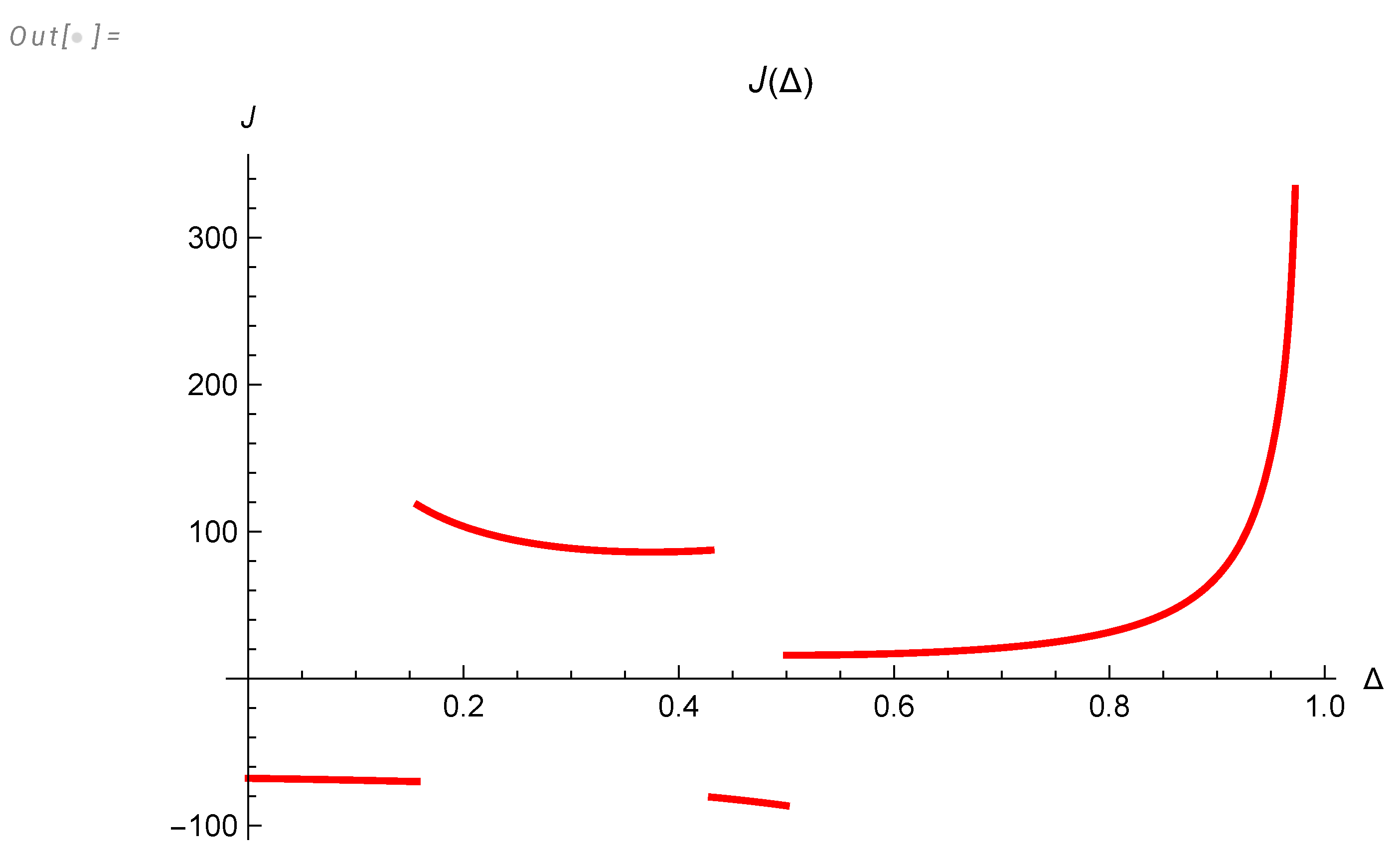
This lowest action root is plotted in Figure 3. The corresponding value of minimal action is plotted in Figure 5.
There are phase transitions at
These branch points in correspond to the switch of the lowest action solution. At small positive
This constraint yields the quadratic relation for the last unknown parameter a in our solution
with universal function presented in [14] and shown in Figure 6).
The resulting integral (up to the pre-exponential factor Q) is equal to
The factor contains two terms:
The first term is the contribution of the classical solution we have just found, and the second term comes from Gaussian fluctuations around this solution.
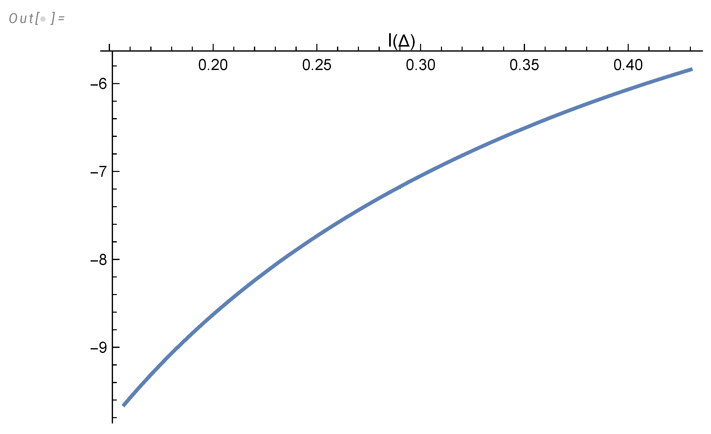
The classical term is calculable (see [14])
This function has an essential singularity at (see Figure 7).
The fluctuation term is also proportional to , therefore we must keep this term as well.
As for the pre-exponential factor Q in the saddle point integral, it is given by the functional determinant of the operator corresponding to linearized effective action (151) in the vicinity of the saddle point .
The fluctuation correction reduces to the inverse operator , which we compute in the next section.
Now, we can reduce multiple sum/integral in (149) to the following
where is the normalization constant to be determined later.
4.3. Functional Determinant in the Path Integral
As we have discussed in the previous section, in the limit the classical solution .
This observation simplifies the linearized theory corresponding to this quadratic form . First, integrate the fluctuations of around the saddle point solution.
The Lagrange multiplier at the saddle point vanishes, as we show in [14]
The quadratic term comes from the first derivatives , which can be simplified by switching to
The bilinear term also simplifies
We can integrate out , producing the extra pre-exponential factor .
The bilinear term in the exponential after integration leads to the following effective quadratic Action for
There is a zero-mode , related to translational invariance of . Naturally, this zero-mode must be eliminated from the spectrum when we compute the functional determinant and the resolvent below.
After discarding the zero-mode, this effective action becomes a positive definite functional of only in the region of where , i.e., for .
As we shall see below, the spectrum of fluctuations is positive only in this region. Therefore, we restrict our integration to this region.
The term corresponds to the linear eigenvalue equation with
The solution matching with first derivative at is built the same way as in (173). Equations for being linear homogeneous, we can fix the normalization as ,
The spectrum is defined by the transcendental equation (the discriminant of this linear system of equations), which we found in [14]
The spectrum is positive in the whole interval except for the region where so that the stable solution for does not exist. In the following, we only select the stable region with positive
Figure 8.
The first levels of the spectrum satisfying equation . The colored lines correspond to four phases. Red: , Green: , Blue: , Brown: . The green zone is left as stable, and others are eliminated because in these zones. Naturally, we eliminate the zero-mode corresponding to translational invariance of the effective Action.
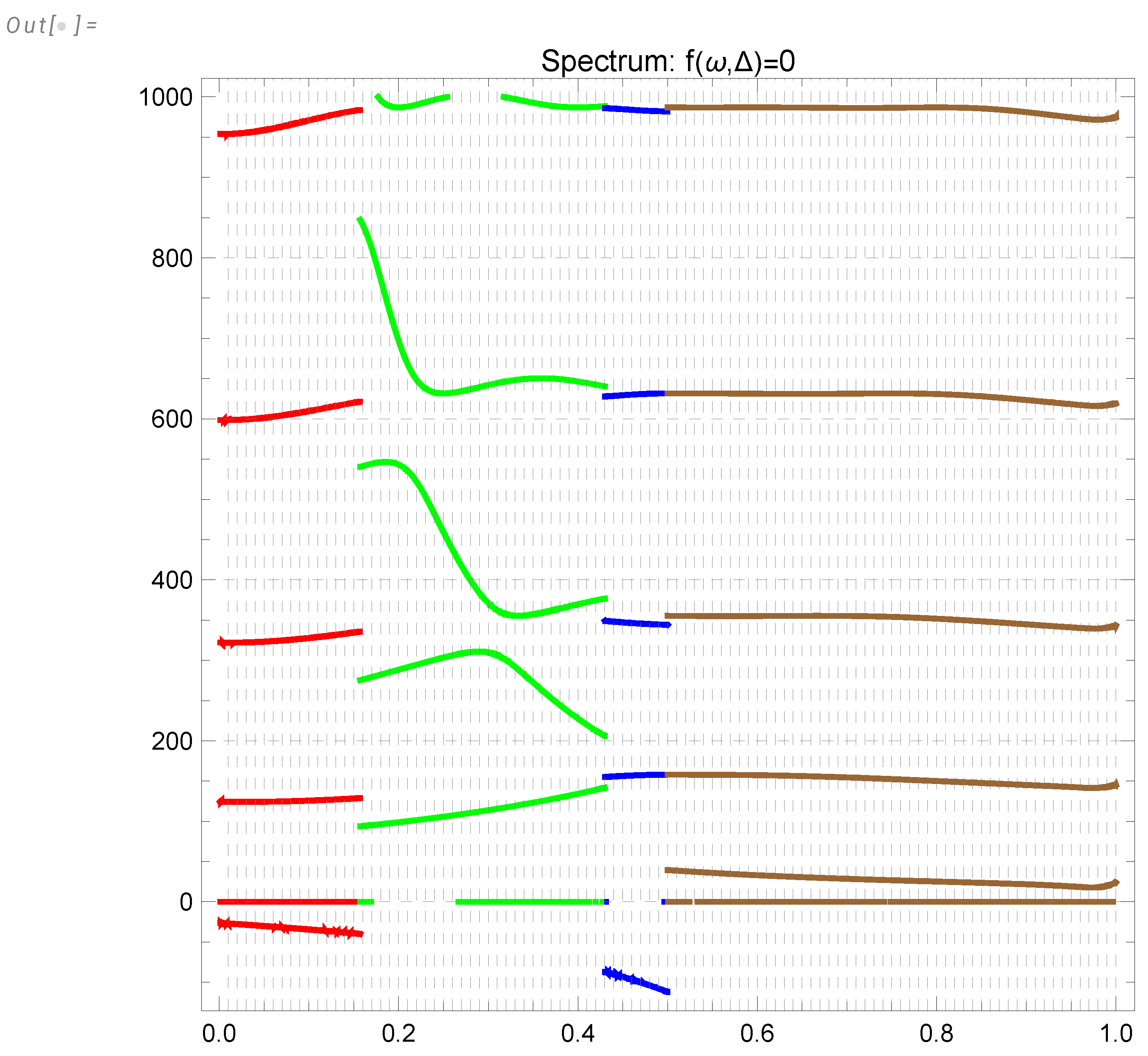
The functional determinant, resulting from the WKB approximation to the path integral, would be related to the infinite product of positive eigenvalues , which can be written using a contour integral
and the integration contour encircles anticlockwise the positive real poles of the meromorphic function . The integral converges at and should be analytically continued to .
For this purpose, let us introduce another function
We show in [14] that at large this function reaches finite limits
The logarithmic derivative of the original function differs from by the following meromorphic function
This difference produces a calculable contribution to our integral. By summing residues of the poles of the tangent, we get
The derivative at yields a constant
leading to an irrelevant renormalization of by a factor .
The remaining integral with already converges at , so that we can set and rotate the integration contour parallel to the imaginary axis at :
The remarkable property of this functional determinant is the factorization of the dependence
The index has a topological origin and can be computed analytically.
Our result for the correlation function is given by (195) with
and given by (218). All the constant factors we have omitted here are absorbed by the normalization factor , which we determine at the end of the next section.
4.4. The Fluctuation Term in
The last missing term is the fluctuation contribution to . In the Gaussian approximation, valid at , this term equals
where is a resolvent for the effective quadratic Action (202). This resolvent satisfies the equation
The solution of this equation, matching with the first derivative at is
The linear functional on this solution becomes a linear function of these unknown parameters . Two boundary conditions fix these parameters as functions of .
The result derived in [14] is too lengthy to present here. The desired quantity (223) is quite simple
Finally, we get the following correlation (195) (absorbing the constant factors in )
5. The Decaying Energy in Finite System
The vorticity correlation in Fourier space doubles as an energy spectrum
The energy spectrum in a finite system with size L is bounded from below. At low , the spectrum is no longer related to the turbulence but is given by the energy pumping by external forces at the boundaries.
This energy pumping [4] takes place at , after which the pumping stops. At this moment, the energy spectrum is growing with wavevector by one of two possible laws (with P being the net momentum of the fluid and M being the rotation moment)
At , without the forcing, the pumped energy dissipates at large k corresponding to smaller spatial scales of the hierarchy of vortex structures of all scales, ending with dissipative scales, or wavevectors . After sufficient time, the universal regime kicks in, corresponding to the decaying turbulence. It is implied that a large amount of energy was pumped in, so it takes a long time to reach this decaying regime, corresponding to some fixed trajectory.
Our solution would apply to this regime. This solution corresponds to zero net momentum, which leaves the second regime with spectrum at small k and some universal decay at large k, reflecting these distributed vortex structures.
Therefore, the decaying energy, given by the part of the spectrum , has the following form
On top of the trivial decrease , as prescribed by dimensional counting in an infinite system, there is some extra decrease related to the increase of the lower limit.
The energy in our theory does not have a finite statistical limit as the integral in (235) diverges at the lower limit when . Thus, we compute the energy as
This energy dissipation rate is calculable
In our theory, this integral has a finite limit in an infinite system ().
This limit was computed in [1] in a slightly different grand canonical ensemble, where N was fluctuating with the weight .
With our current ensemble of fixed even the results of [1] read:
In our present theory, the same quantity is given by the above integral at
Comparing these two expressions, we get the normalization of
The integral on the left can be further reduced [14] to the following normalization condition:
This normalization constant can be used in equation (235) for the energy decay in a finite system. All the functions of were defined above.
As for the energy spectrum, this is not an independent function in our theory. Comparing the two expressions (233) and (237), we arrive at the following relation
Both the energy dissipation and the energy spectrum are related to the same function , but the energy spectrum related to the derivative of this function at large argument , whereas the energy dissipation is related to the value of this function at small argument .
There is no single power decay, as the quantum effects related to integration over and summation over rational numbers will produce a superposition of power laws with various slopes.
We computed the effective decay index
numerically in the Appendix, using Mathematica®. The accuracy is just 4-5 digits, but it can be easily improved by taking more CPU time once experimental data gets more precise. This curve is universal, apart from an arbitrary time scale (measured in ).
The effective index grows, starting around at (with artificial initial point and scale ) and asymptotically reaching at , covering the same range as experimental data [4].
This asymptotic index corresponds to resulting in asymptotic spectrum
Current data for the energy decay index n [4] are inconsistent. There are large discrepancies between various experiments, which are presumably explained by attempts to fit the energy decay to a single power. In our theory, the energy decay is a nonlinear function on the log-log scale.
The best approach to experimental data is to present it as an effective curve , as it was done in [4] and presented here in Figure 10 with permission from Sreeni.
One of these curves (the green one) closely matches our theoretical prediction in Figure 9.
Numerical computation of this universal function in [14] yields the curve in Figure 11, Figure 12, Figure 13.
Figure 9.
Green curve is the effective index as a function of time, shifted and rescaled to match the experimental time range. The derivatives were taken using the 5th-order interpolation of computed values at 60 points. Asymptotically, at it reaches .
Figure 9.
Green curve is the effective index as a function of time, shifted and rescaled to match the experimental time range. The derivatives were taken using the 5th-order interpolation of computed values at 60 points. Asymptotically, at it reaches .
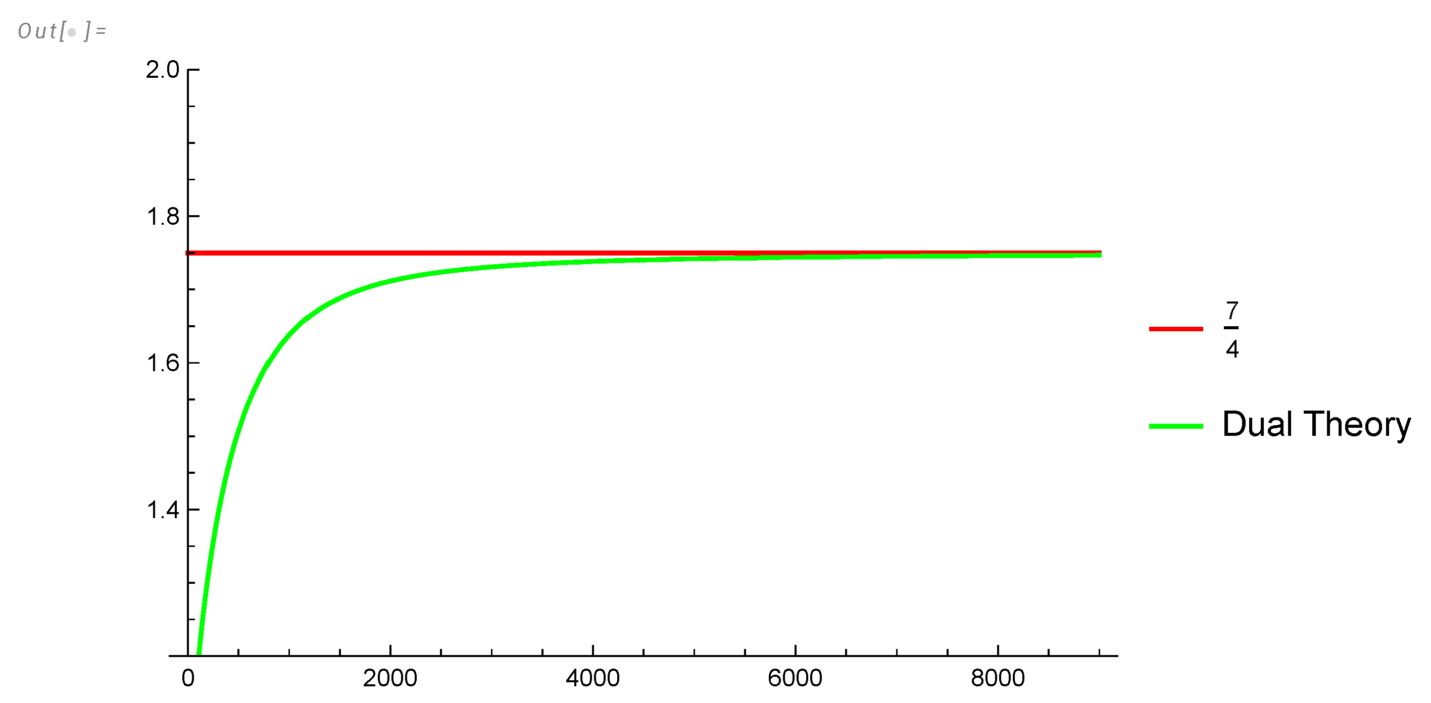
Figure 10.
Data for effective index as compiled in [4]. The green curve matches our prediction in Figure 9.
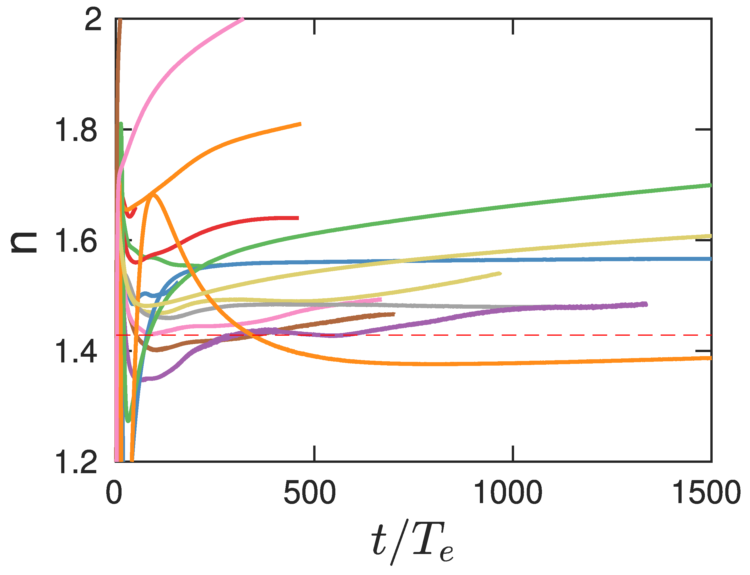
Figure 11.
Universal function which determines both the energy decay and the energy spectrum in ().
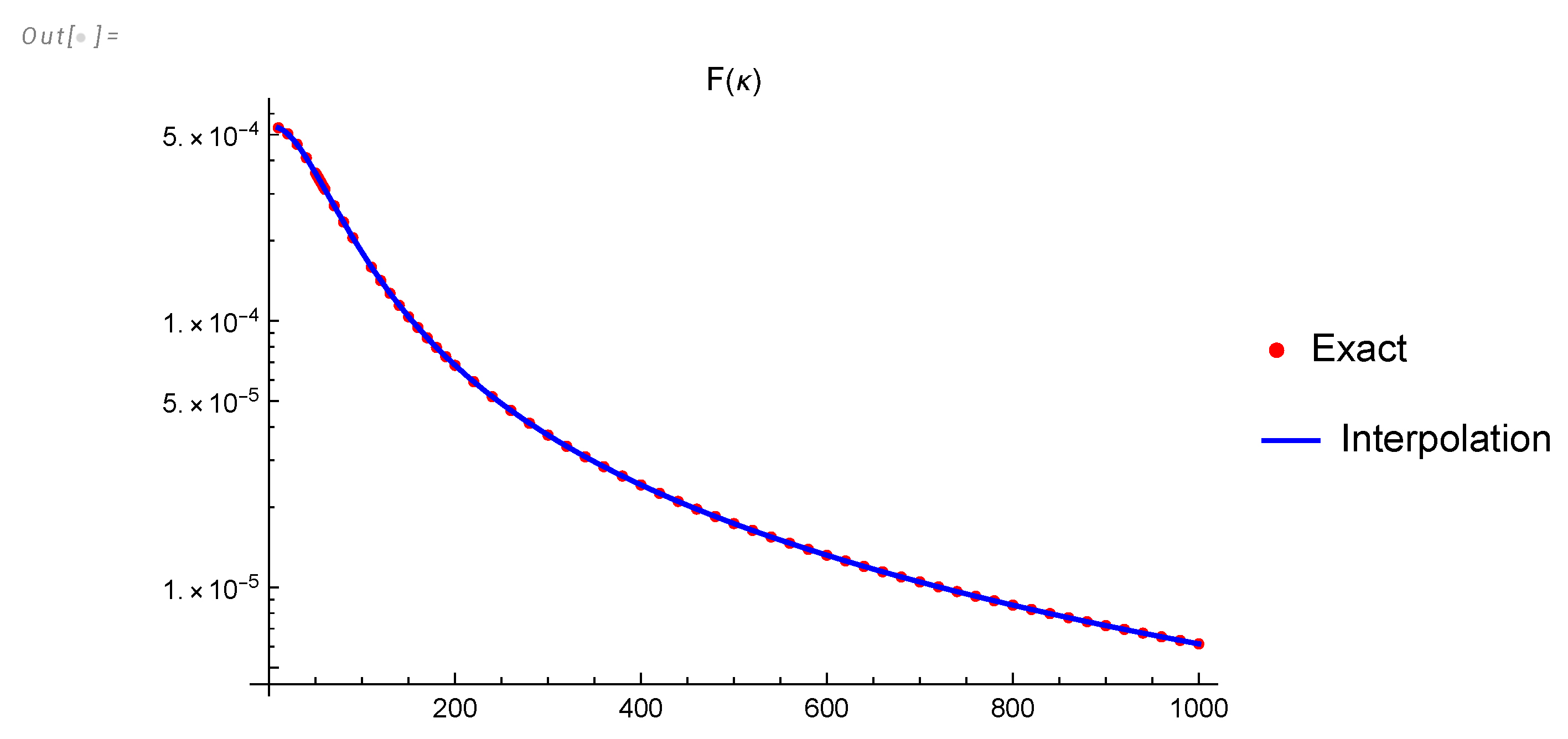
Figure 12.
Log-log plot of the energy spectrum as a function of wavevector k in dual theory of decaying turbulence. The effective slope is changing with scale and reaches limit
Figure 12.
Log-log plot of the energy spectrum as a function of wavevector k in dual theory of decaying turbulence. The effective slope is changing with scale and reaches limit
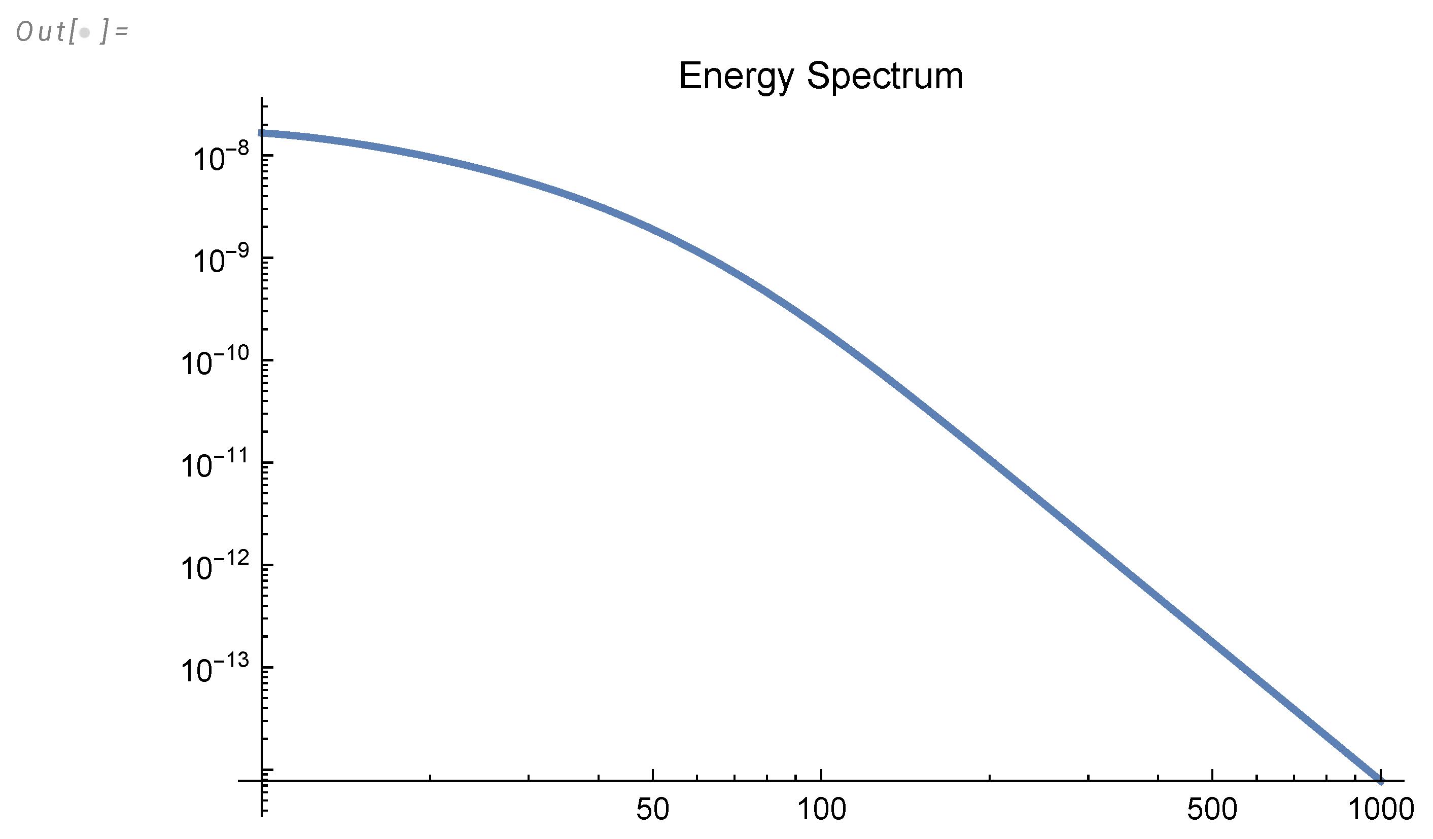
Figure 13.
Effective index as a function of k.
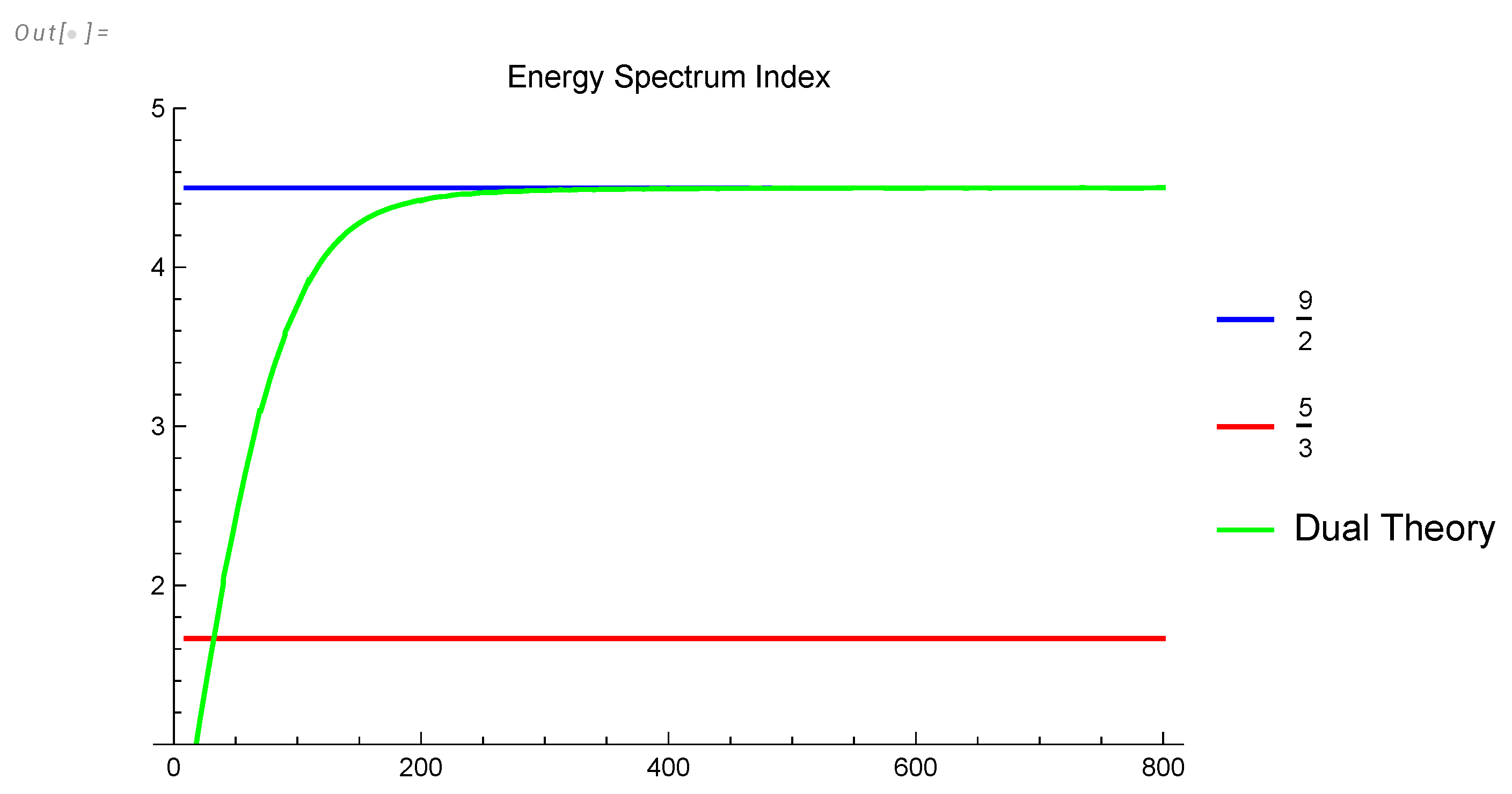
According to the dual theory, the energy decay index will grow, pass the K41 value, and saturate at .
Our theory has no dimensionless parameters to fit: these universal curves were computed directly from the analytic solution of the loop equation in the turbulent limit .
6. Summary
Here are the new results reported in this paper.
- We found the continuum limit of distribution of scaling variables (125) in the small Euler ensemble.
- We reduced the Markov process for the Euler ensemble in its fermionic representation (61) to the path integral.
- We solved this classical equation corresponding to the vorticity correlation function and found the spectrum of the linear operator for small fluctuations around this solution.
- We computed the contribution of the instanton to the vorticity correlation function by using zeta regularization of the functional determinant of this linearized operator.
- The continuum limit of this solution, , corresponds to the inviscid limit of the decaying turbulence in the Navier-Stokes equation. Effective turbulent viscosity is .
7. Remaining Problems
- We performed all the calculations up to numerical factors in the vorticity correlation function, which we recovered from the previously computed (see [1] ). It would be useful to compute all the normalization factors and thus double-check the solution.
- The spectrum of decay indexes for deviations from our fixed trajectory [1] can be evaluated in the scaling limit, with finite .
-
Another solvable problem is the PDF of the velocity circulationThe dependence is absent in the leading term of the solution, so the correction term must be computed, like in [1], with the corresponding decay index at a large time. The PDF of the velocity circulation was measured in [15,16] and explained as an instanton in [8]. Computing it from first principles would be an important achievement.
Funding
The author is supported by a Simons Foundation award ID 686282
Data Availability Statement
Acknowledgments
Yang-Hui and I discussed Euler’s totients at the Cambridge University workshop, where this theory was first reported in November 2023. His comments helped me derive the asymptotic distribution for scaling variables. I am also grateful to the organizers and participants of the "Field Theory and Turbulence " workshop at ICTS in Bengaluru, India, where this work was advanced in December 2023. Discussions with Katepalli Sreenivasan, Rahul Pandit, and Gregory Falkovich were especially useful. They helped me understand the physics of decaying turbulence in a finite system and match my solution with the DNS data. Recently, this work was discussed at the "Conformal Field Theory, Integrability, and Geometry" conference in Stony Brook in March 11-15, 2024. I am very grateful to Nikita Nekrasov, Sasha Polyakov, Sasha Zamolodchikov, Dennis Sullivan and other participants for deep and inspiring discussions. This research was supported by a Simons Foundation award ID 686282 at NYU Abu Dhabi. The computations were done on the High-Performance Computing resources at New York University Abu Dhabi.
Appendix A. Computation of Energy Spectrum and Dissipation
We have derived the analytic formula for the energy decay in quadrature. Using Mathematica®, all the involved integrals can be computed numerically with arbitrary precision. This computation is the purpose of this Appendix.
First of all, we can analytically integrate the equation for the energy dissipation rate over the variable
This function W reduces to an error function , polynomial, and exponential (see [14]).
Its value at and its sum over n with Euler totient are finite and calculable
We use these exact values to accelerate the convergence of the sum over n
The normalization constant was computed in [14] by numerical integration over :
Restoring the normalization produces a well-defined expression involving an error function, an exponential integral, and Euler totients. The hardest part of the calculation is the integral in exponential for in (218). After regularization, it converges, but there are some oscillations on top of the power decay of the integrand.
Figure A1.
The function related to .
We used the Mathematica® integration by the method "DoubleExponentialOscillatory" [17], which applies to oscillating functions in the infinite interval.
The remaining sum over n with the weight converges at infinity; we compute it utilizing the "NSum" method of Mathematica®. This method extrapolates to the finite sum up to . With the Euler totient this extrapolation converges slowly, which increases the CPU time.
Still, we compute this function fixed for . Next, we have to integrate over , which we did numerically, interpolating the values at the grid with the step . The estimated error is about the same as the accuracy of our integral for Q.
We preprocessed the table of values of the integral
fine in the exponential in at the fine grid with step in the integration range . Then, we used third-order interpolation to further integrate over . This function has no singularities in the integration region and is close to the second-order polynomial. Therefore, our cubic interpolation over the grid with step produces very accurate results.
The remaining functions are either elementary or the solution of a trigonometric equation, so we know them with arbitrary accuracy.
We tabulated on a grid of with the step . The function behaved smoothly so that the fifth-order polynomial interpolation produced small errors (less than ).
The effective index and the other two plots were obtained by analytical differentiation of this fifth-order interpolation. Results were presented above, in Figure 11,12,13, 9.
The computations were performed on a laptop, with precision more than sufficient to compare with existing experiments. Running the same code [14] with smaller steps on a supercomputer would yield higher precision results for effective indexes.
References
- Migdal, A. To the Theory of Decaying Turbulence. Fractal and Fractional 2023, arXiv:physics.flu-dyn/2304.13719]7, 754. [Google Scholar] [CrossRef]
- Migdal, A. Loop Equation and Area Law in Turbulence. In Quantum Field Theory and String Theory; Baulieu, L., Dotsenko, V., Kazakov, V., Windey, P., Eds.; Springer US, 1995; pp. 193–231. [Google Scholar] [CrossRef]
- Basak, D.; Zaharescu, A. Connections between Number Theory and the theory of Turbulence, 2024. To be published.
- Panickacheril John, J.; Donzis, D.A.; Sreenivasan, K.R. Laws of turbulence decay from direct numerical simulations. Philos. Trans. A Math. Phys. Eng. Sci. 2022, 380, 20210089. [Google Scholar] [CrossRef]
- Migdal, A. Topological Vortexes, Asymptotic Freedom, and Multifractals. MDPI Fractals and Fractional, Special Issue, 2023; arXiv:physics.flu-dyn/2212.13356]. [Google Scholar]
- Matsuzawa, T.; Irvine, W. Realization of Confined Turbulence Through Multiple Vortex Ring Collisions, 03/12/2019, [https://www.quantamagazine.org/an-unexpected-twist-lights-up-the-secrets-of-turbulence-20200903/]. "Talk at the Flatiron Conference Universality Turbulence Across Vast Scales".
- Matsuzawa, T.; Mitchell, N.P.; Perrard, S.; Irvine, W.T. Creation of an isolated turbulent blob fed by vortex rings. Nature Physics 2023, 19, 1193–1200. [Google Scholar] [CrossRef]
- Migdal, A. Statistical Equilibrium of Circulating Fluids. Physics Reports 2023, arXiv:physics.flu-dyn/2209.12312]1011C, 1–117. [Google Scholar] [CrossRef]
- AGISHTEIN, M.; MIGDAL, A. SIMULATIONS OF FOUR-DIMENSIONAL SIMPLICIAL QUANTUM GRAVITY AS DYNAMICAL TRIANGULATION. Modern Physics Letters A 1992, 07, 1039–1061. [Google Scholar] [CrossRef]
- Hardy, G.H.; Wright, E.M. An introduction to the theory of numbers, Revised by D. R. Heath-Brown and J. H. Silverman, With a foreword by Andrew Wiles, 6th ed.; Oxford University Press: Oxford, UK, 2008; pp. xxii+621. [Google Scholar]
- Bulatov, M.; Migdal, A. Dual Theory of Decaying Turbulence.2. Numerical Simulations.
- Norris, J.R. Markov chains; Cambridge Univ. Press, 2007. [Google Scholar]
- Migdal, A. "BernSum". "https://www.wolframcloud.com/obj/sasha.migdal/Published/BernSum.nb", 2024.
- Migdal, A. "InstantonComputations". "https://www.wolframcloud.com/obj/sasha.migdal/Published/JacobiEllipticForDecayingTurbulence.nb", 2024.
- Iyer, K.P.; Sreenivasan, K.R.; Yeung, P.K. Circulation in High Reynolds Number Isotropic Turbulence is a Bifractal. Phys. Rev. X 2019, 9, 041006. [Google Scholar] [CrossRef]
- Iyer, K.P.; Bharadwaj, S.S.; Sreenivasan, K.R. Area rule for circulation and minimal surfaces in three-dimensional turbulence. 2020; arXiv:physics.flu-dyn/2007.06723]. [Google Scholar]
- MORI, M.; OOURA, T. Double exponential formulas for Fourier type integrals with a divergent integrand. In Contributions in Numerical Mathematics; World Scientific, 1993; pp. 301–308. [Google Scholar]
| 1 | Nikita Nekrasov (private communication) suggested to me an algorithm of generating this solution as a set of adjacent triangles in complex 3-space and pointed out an invariant measure in phase space, made of lengths of shared sides and angles between them. Unfortunately, this beautiful construction does not guarantee real circulation, requiring further refinement. |
Figure 1.
The plot of the function . As required, it is positive, takes a maximal value at , and vanishes at both ends of the physical region.
Figure 1.
The plot of the function . As required, it is positive, takes a maximal value at , and vanishes at both ends of the physical region.
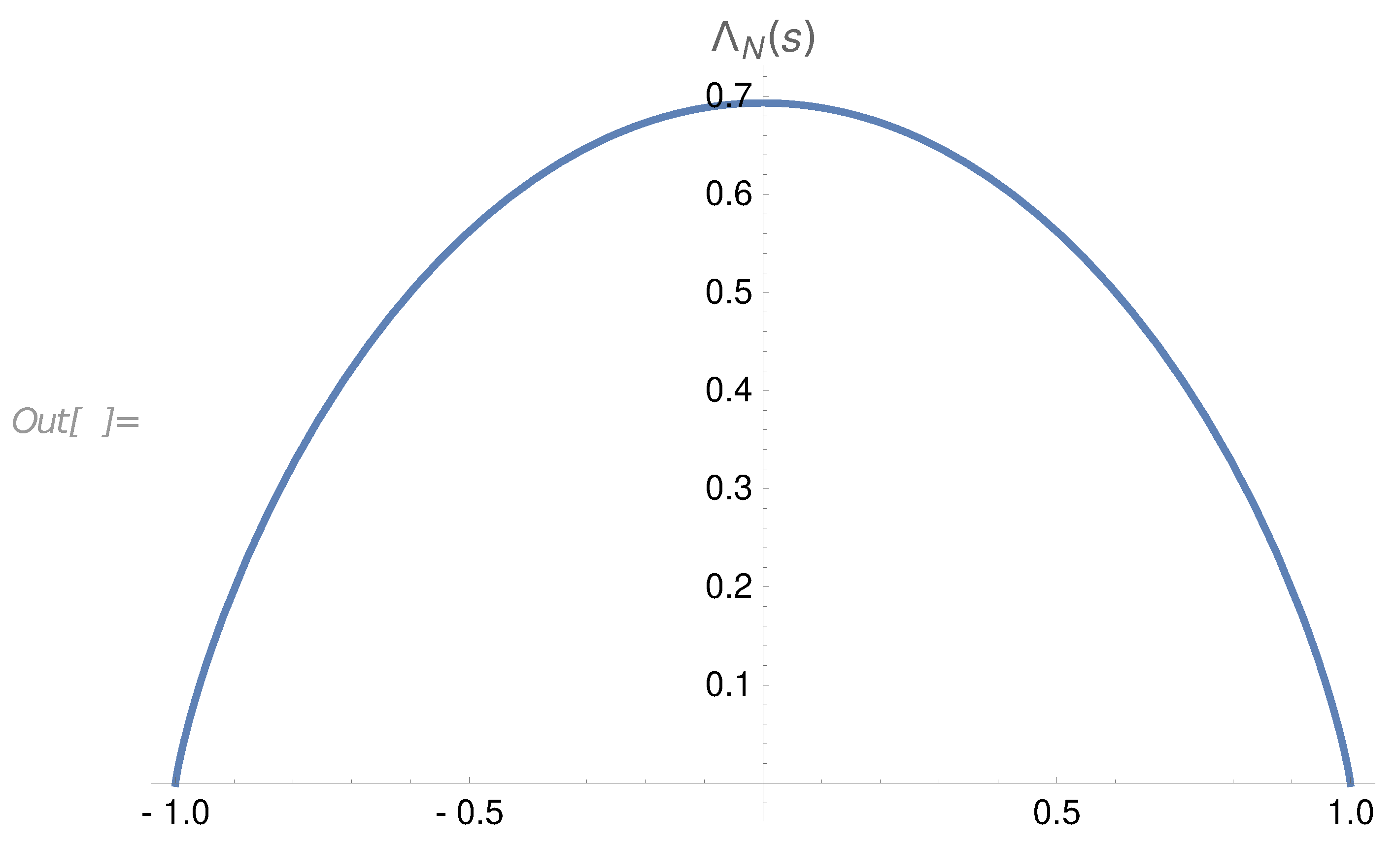
Figure 2.
The log-log-plot of the distribution . It is equals at each internal with positive integer k. Asymptotically at .
Figure 2.
The log-log-plot of the distribution . It is equals at each internal with positive integer k. Asymptotically at .
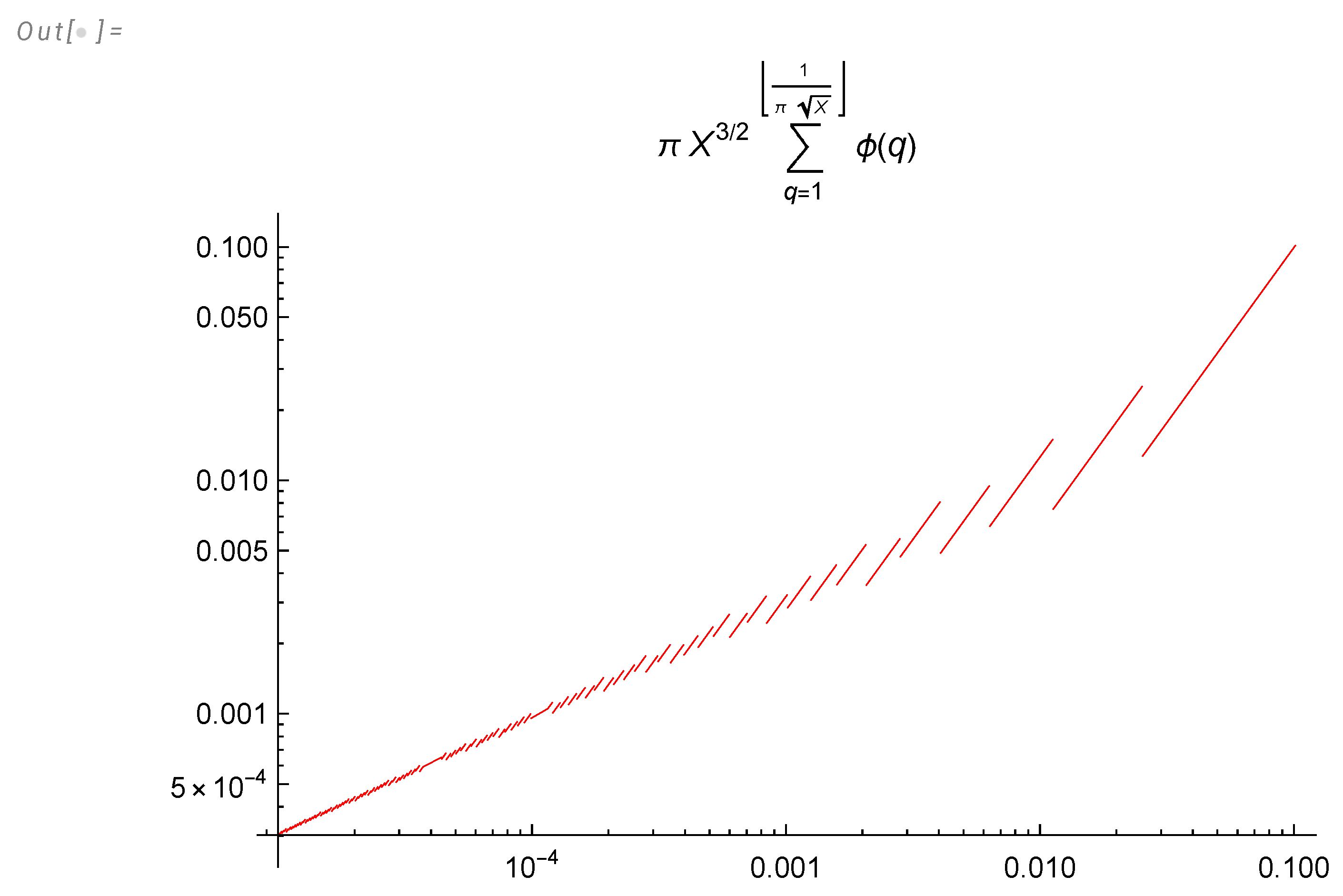
Figure 3.
Log plot of
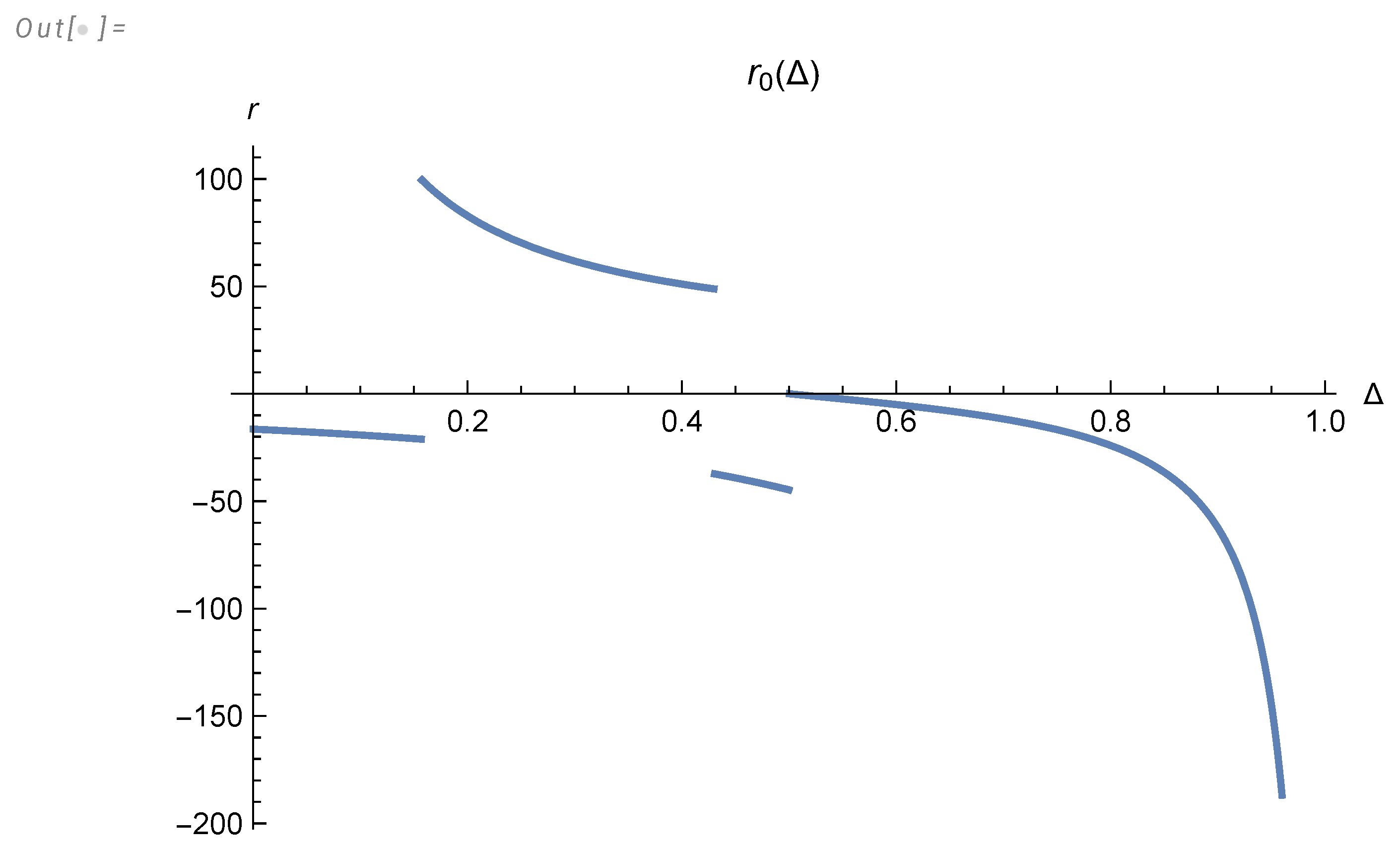
Figure 4.
Plot of for the three real solutions of the equation . At and , the action curves intersect; at , there is a gap between the lowest action () and the lowest of the other two. So, there are second-order phase transitions at and the first-order phase transition at .
Figure 4.
Plot of for the three real solutions of the equation . At and , the action curves intersect; at , there is a gap between the lowest action () and the lowest of the other two. So, there are second-order phase transitions at and the first-order phase transition at .
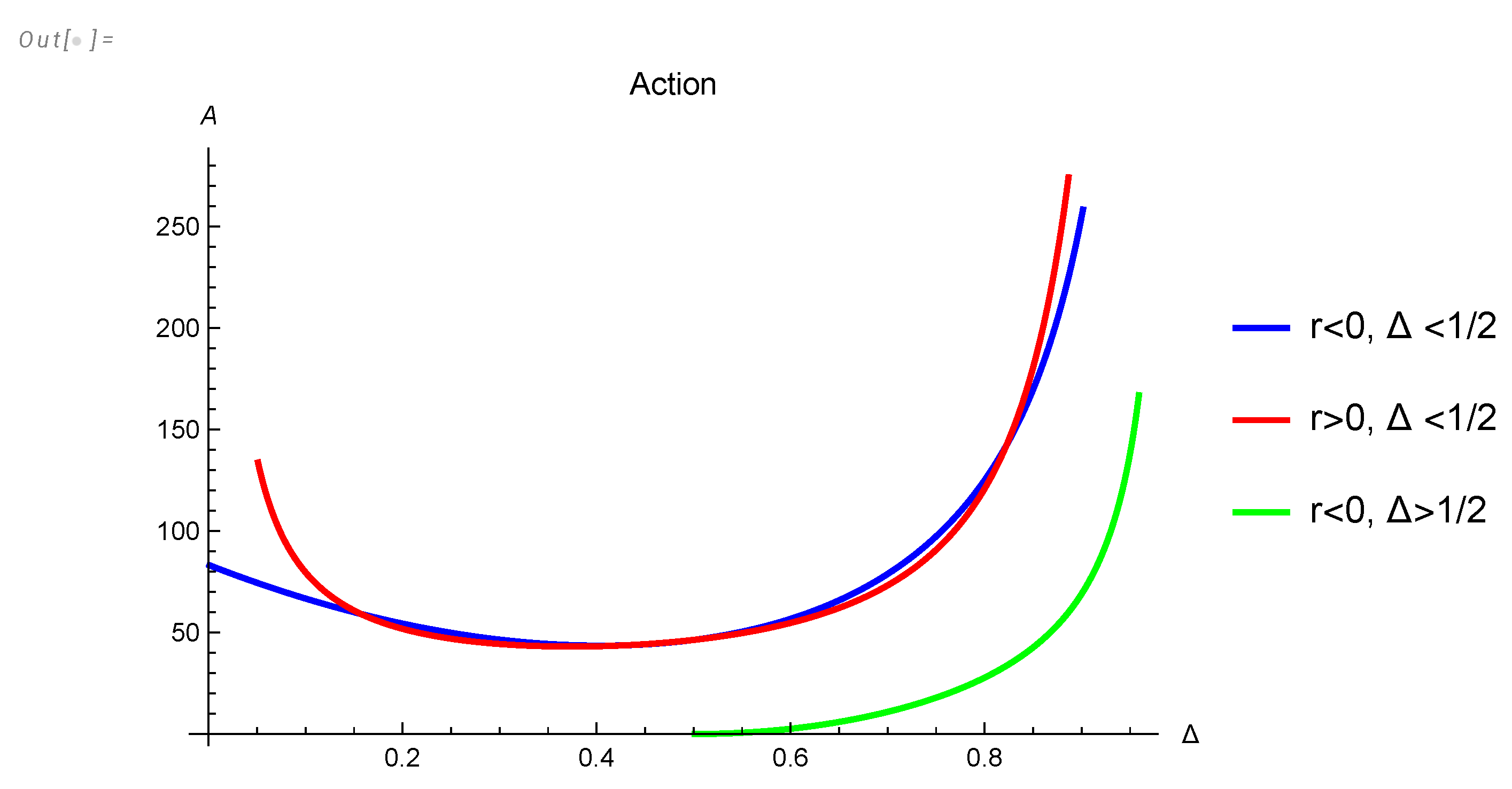
Figure 5.
Log plot of .
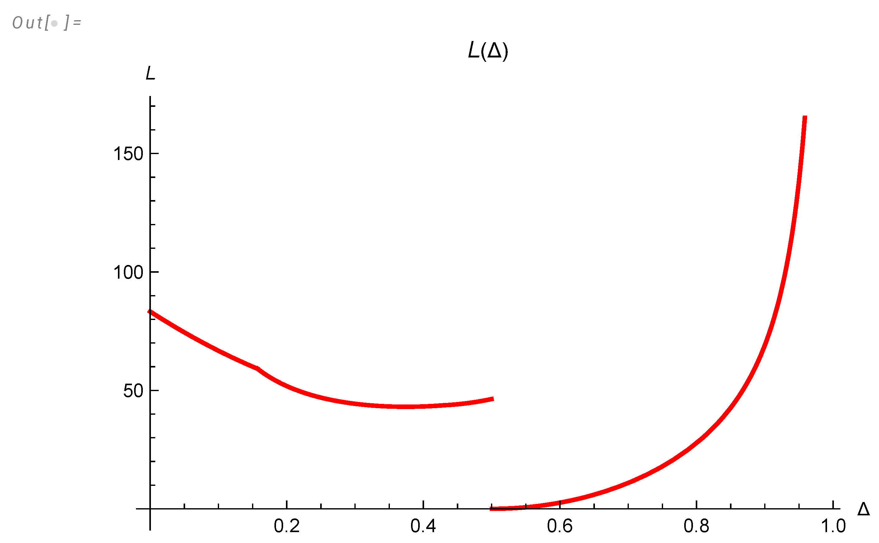
Figure 6.
Plot of .
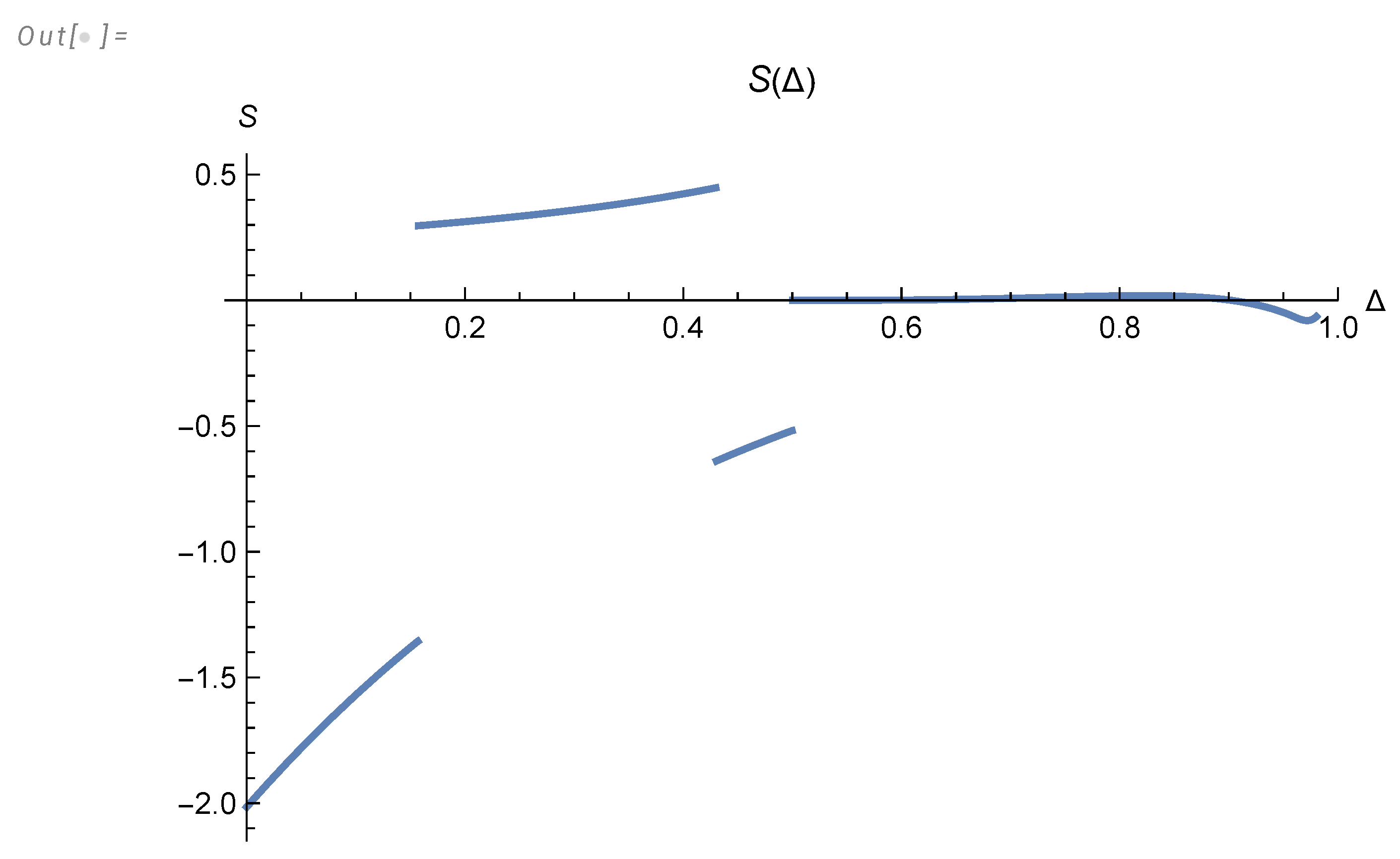
Figure 7.
Plot of universal function .the four corves correspond to four phases (solutions for ).
Disclaimer/Publisher’s Note: The statements, opinions and data contained in all publications are solely those of the individual author(s) and contributor(s) and not of MDPI and/or the editor(s). MDPI and/or the editor(s) disclaim responsibility for any injury to people or property resulting from any ideas, methods, instructions or products referred to in the content. |
© 2024 by the authors. Licensee MDPI, Basel, Switzerland. This article is an open access article distributed under the terms and conditions of the Creative Commons Attribution (CC BY) license (http://creativecommons.org/licenses/by/4.0/).
Copyright: This open access article is published under a Creative Commons CC BY 4.0 license, which permit the free download, distribution, and reuse, provided that the author and preprint are cited in any reuse.


