1. Introduction
Turbulence remains one of the deepest unsolved problems in classical physics. The standard approach to turbulence relies on heuristic scaling laws, such as Kolmogorov’s 1941 (K41) model, which describe statistical properties of turbulent flows but do not derive them directly from the NS equations. Despite advances in numerical simulation, a rigorous mathematical framework for turbulence remains elusive, and the Millennium Problem on NS regularity remains open, with no general proof of whether solutions develop singularities or remain smooth for all time.
Here, we present a fundamentally new formulation of fluid mechanics:
The Navier-Stokes system in 3D can be rewritten as a singular one-dimensional nonlinear equation in loop space.
This momentum loop equation (MLE) transforms fluid dynamics from a high-dimensional PDE into a solvable nonlinear dynamical system.
As a direct consequence of this formulation, we derive a No Explosion Theorem, proving that finite-time singularities do not occur under stochastic initial conditions.
A special solution of the MLE, the Euler ensemble, provides an exact solution to a boundary value problem, describing the asymptotic behavior of decaying turbulence.
1.1. Dimensional Reduction of the Navier-Stokes System
The key breakthrough of this work is the discovery that the entire Navier-Stokes problem can be formulated in terms of a momentum loop equation. This transformation rewrites fluid dynamics in loop space, reducing the problem from a 3D nonlinear PDE to a one-dimensional singular equation. Unlike traditional statistical approaches to turbulence, this formulation provides an explicitly solvable structure, revealing new mathematical connections between fluid mechanics, number theory, and quantum systems.
1.2. No Explosion Theorem and Implications for the Millennium Problem
A direct application of this formalism is the derivation of a No Explosion Theorem, which rigorously excludes finite-time singularities for NS flows with stochastic initial data. While this does not yet constitute a full proof of the NS regularity problem (which requires deterministic initial conditions), the limit of vanishing noise may provide a path toward a complete proof. This result provides the first rigorous indication that turbulence does not lead to singular behavior, strengthening the case for NS global regularity.
1.3. Decaying Turbulence and the Euler Ensemble
As a specific application of this formalism, we present an exact solution of the MLE, known as the Euler ensemble. This solution describes a boundary value problem, characterizing the asymptotic state of decaying turbulence in the infinite-time limit. The Euler ensemble replaces heuristic turbulence models with an analytically derived structure, validated against numerical simulations and experimental data.
However, the Euler ensemble is not the most general solution of the MLE. It describes a particular class of turbulent flows, but it remains an open question whether it represents the universal attractor of turbulence. Further work is required to determine whether all turbulent flows evolve toward this structure or whether alternative attractors exist.
1.4. Outline of This Paper
The remainder of this paper is structured as follows. In Section 2, we introduce the momentum loop equation and derive its structure from the Navier-Stokes system. Section 3 presents the derivation of the No Explosion Theorem and discusses its implications. In Section 4, we analyze the Euler ensemble as an exact solution of the MLE and compare its predictions with experimental data. Finally, in Section 5, we discuss open questions, including the extension of our results to deterministic initial conditions, which may lead to a resolution of the Millennium Problem.
This work provides a fundamentally new perspective on fluid dynamics. By reducing the Navier-Stokes system to a solvable one-dimensional equation, we open the door to solving longstanding problems in turbulence and fluid mechanics, with implications reaching beyond classical physics.
2. Loop Functional and Its General Properties
The loop functional is defined as a phase factor associated with velocity circulation, averaged over the initial distribution
of the velocity field
We use viscosity
as a unit of circulation. Both have the same dimension
as the Planck’s constant
ℏ. The viscosity will play the same role in our theory as Planck’s constant in quantum mechanics. The variable
with this definition is dimensionless.
This loop functional is the Fourier transform of the PDF for the circulation over fixed loop
C
There is an implicit dependence of time, coming from the evolution of the velocity field by the Navier-Stokes equation
We restrict ourselves to three-dimensional Euclidean space, the most interesting case for physics applications. The generalization to arbitrary dimension is straightforward, as discussed in previous papers [
1,
2,
3].
In the next sections, we shall study the Cauchy problem for the loop equation [
1,
2], which follows from the Navier-Stokes equation. Here, we state some general properties of the loop function and various scenarios of its evolution.
The first obvious property is that this evolution goes inside the unit circle
At a small enough time passed from initial data,
, turning off the noise would bring us to the usual unique laminar solution of the Navier-Stokes equation, corresponding to the loop functional at the unit circle with a small enough phase.
Here,
denotes the variance of the Gaussian distribution of the velocity field around some smooth initial value. Generally speaking, we could expect the following fixed points (see
Figure 1) of the time evolution for the loop functional
1.
In the following sections, we elaborate on each of these possible regimes. The finite-time explosion is proven to be inconsistent and is therefore ruled out.
3. Loop Equation
The first step is to write down the loop equation by projecting the Hopf equation [
5] to the loop space.
Before doing that, we have to specify certain boundary conditions which we assume in our fluid dynamics. Namely, we consider infinite space , with boundary condition of vanishing or constant velocity at infinity.
Vorticity can exist throughout the entire spatial domain, but it vanishes at infinity, as required by our boundary conditions, where velocity gradients diminish. We also assume the absence of internal boundaries, such as solid surfaces that the fluid flows around. However, we allow for the presence of singular regions of vorticity, such as vortex lines and sheets, in the inviscid limit, provided these regions are confined to a finite portion of the volume, consistent with our boundary conditions.
At finite viscosity, these singular regions may acquire a finite thickness proportional to , leading to anomalous dissipation in turbulent flows.
An alternative, simpler mechanism for anomalous dissipation arises when velocity increases as viscosity vanishes, even in the absence of singular vortex structures like Burgers vortices. In this scenario, the turbulent energy grows as viscosity decreases, while the spatial distribution of vorticity remains homogeneous and non-singular.
As we will demonstrate below, this is the mechanism realized in our solution for decaying turbulence.
The computations leading to the loop equation were performed in the old papers [
1,
2]. For the reader’s convenience, we repeat them here using another language, hopefully more clear for mathematicians.
The straightforward time derivative of the loop functional, assuming the constant loop
C and using time derivative (
5) of the velocity field in the circulation, yields
The averaging
goes, as before, over time-dependent NS solutions
with a given set of initial values
. It is implied that a probability measure (see examples below) is supplied for this set of initial velocity fields. The phase factor of circulation is averaged over initial data using this measure.
The gradient terms
in (
5) dropped in the time derivative of the circulation as the integral of a gradient of some single-valued function of coordinate
around the closed loop:
The velocity field
is a solution of the Poisson equation, relating it to vorticity by incompressibility condition
This representation leaves vorticity as the main unknown variable in the time derivative of the loop functional.
To find the loop equation, we must replace the vorticity and its gradients with certain operators acting on the loop independently of the vorticity and velocity fields. As a result of such transformation, the vector function
will be replaced by a certain operator
in loop space acting on
This operator
depends on certain operators
instead of on the dynamical variables
, therefore it can be taken out of the averaging over trajectories starting from various initial data
so that this operator acts on the loop average
. Such is the plan of the proof of the loop equation. We define the loop operators and follow this plan in the next section.
4. The Definitions of the Loop Operators and the Proof of the Loop Equation
The operators in the loop equation were introduced in[
1] and explained at length in my review paper[
2].
In this paper, we do not assume any knowledge of the previous work; instead, we derive the loop operators from scratch using a simpler method.
First, we approximate the smooth loop by a polygon with N vertices in the limit . We postpone this local limit until we solve the discrete loop equation. This limit will define the continuum theory in the same way as in the QFT; the functional integral is discretized using a lattice with the lattice spacing going to zero at the end of the calculation. In this limit, the theory’s parameters vary with the lattice spacing to provide a finite result for the physical observables.
The first observation is that with smooth velocity and vorticity fields, the discrete circulation around the polygon
converges to the circulation around the smooth loop
The line integral
becomes the continuous integral along the loop
C in the limit
when the sides
of the polygon tend to zero.
The next property is also easy to prove using the Stokes theorem for a small triangle
To prove this we rewrite the complete circulation as a sum of two:
The circulation
corresponds to the loop with one vertex
removed, resulting in a side connecting
directly to
. The other term
corresponds to circulation around the triangle made of three vertices
. When these two circulations are added, the line integral
cancels between the two, so we are left with original circulation over complete polygon
C.
The derivatives by only involve the triangle circulation and are easily estimated at .
This first derivative vanishes at as .
The second derivative, however, stays finite. We prefer to use another set of variables
The last relation follows from the chain rule
The vorticity can be represented as
The contour C becomes an open line when we move all independently, without restricting . However, the contribution to the time derivative of circulation from the extra gap between the endpoints where is the enthalpy, which is supposed to be differentiable. Thus, this error term goes to zero as we reinstate the closure condition .
Finally, the velocity field at the vertex
can be related to the vorticity through the Biot-Savart law
Let us verify this relation using the Biot-Savart integral formula for the inverse Laplace operator
At first glance, the loop in the new circulation
involves two long "wires":
and
.
However, in the local limit, when the distance
, these two wires have zero area inside the arising thin triangle, so they effectively cancel in virtue of the Stokes theorem, assuming the Biot-Savart integral converges.
This produces the desired result in the Biot-Savart formula.
The convergence of the Biot-Savart integral follows from our boundary conditions, assuming no vorticity at infinity or even stronger requirement of finite support of vorticity. The phase factor does not influence the absolute convergence, so it can be set to for that purpose and taken out of the integral, returning us to the convergence of the ordinary Biot-Savart integral.
Therefore, with
accuracy, we can replace the right side of the (
10) by its discrete version with operators involving
We restrict ourselves to the velocity vanishing at infinity and no internal boundaries in the physical domain. With this boundary condition, the harmonic potential is zero, and there is no zero mode to add to the inverse Laplace operator.
In the rest of the paper, we shall use the language of the continuum theory, implying the limit of a polygon with N sides. While the lengths of the sides of vanish in the local limit , the sides of polygon are not at our disposal, so they may stay finite (this will happen in the decaying turbulence below).
5. Schrödinger equation in loop space
Before we investigate the solutions of the loop equation, let us consider its physical and mathematical meaning and its relation to the geometry of the incompressible flow.
By definition, the loop functional is a superposition of the phase factors with the circulation of a particular solution of the Navier-Stokes equation. These solutions have initial values , distributed by some distribution which we assume Gaussian with the mean given by some smooth initial field and some coordinate-independent variance .
In the turbulent scenario, the Navier-Stokes trajectories initiated from a narrow vicinity of some smooth velocity field eventually expand and cover some attractor, slowly varying with time and asymptotically converging to .
The alternative smooth solution of the Navier-Stokes equation, sought after in numerous mathematical papers, would correspond to these trajectories staying close and converging to a single trajectory in the limit . This single trajectory would go along the unit circle, bounding our disk.
With this generalization of a definition of the Cauchy problem for the Navier-Stokes equation, we can address the existence of smooth, explosive, or stochastic (i.e., turbulent) solutions within the loop equation’s framework.
The transformation from the Navier-Stokes equation to the loop equation is similar to that from the Newton equation of the particle in random media to the diffusion equation. We add dimension to the problem, switching to the probability distribution in , after which the particle’s infinitesimal time steps translate into probability derivatives by coordinates.
There are two essential differences, however. Our loop space is not just higher-dimensional; in the local limit , it is infinite-dimensional. The second difference is that in addition to diffusion terms , we have nonlocal advection terms affecting the evolution of the distribution in loop space.
Our definition of the loop functional already by construction has superficial similarities with quantum mechanics. We are summing phase factor over a manifold of solutions of the Navier-Stokes equations. The circulation plays the role of classical Action, and viscosity plays the role of Planck’s constant.
This analogy becomes a complete equivalence when the time derivative of the loop functional is represented as an operator in the loop space acting on this functional.
Now we have quantum mechanics in loop space, with the Hamiltonian
The operator
depends of functional derivatives
, as was determined, and discussed in previous works [
1,
2,
3]. Our polygonal approximation has no functional derivatives, just ordinary derivatives
. Thus, our quantum-mechanical system has
continuum degrees of freedom
with periodicity constraint
.
This Hamiltonian is not Hermitian, which reflects the dissipation phenomena. The time reversal leads to complex conjugation of the loop functional, a nontrivial transformation, as there is no symmetry for the reflection of velocity field .
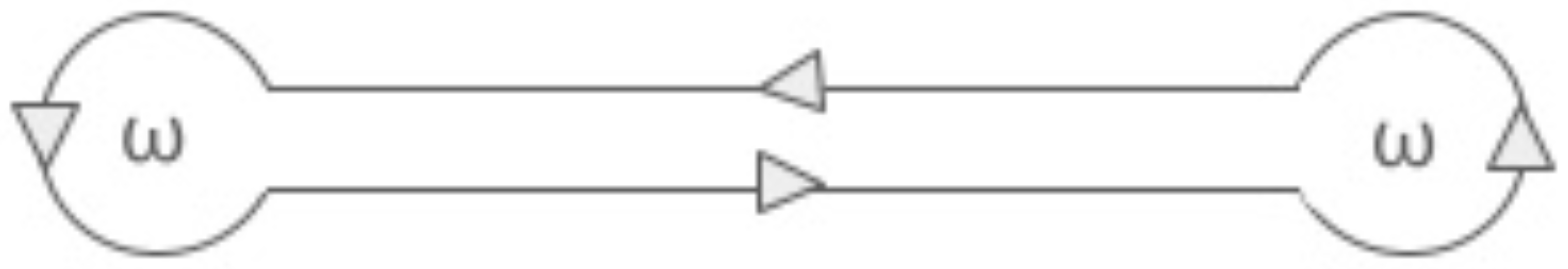
The loop in our theory is a periodic function of the angular variable
. Geometrically, this is a map of the unit circle into Euclidean space
. In particular, there could be several smaller periods, in which case this loop becomes a set of several closed loops connected by backtracking wires like in
Figure 2.
Also, this map could have an arbitrary winding number n corresponding to the same geometric loop in traversed n times.
The linearity of the loop equation is the most important property of this transformation from Navier-Stokes equation to the quantum mechanics in loop space.
This transformation exemplifies how the nonlinear PDE reduces to the linear problem projected from high dimensional space. In our case, this space is the loop space, which is infinite-dimensional.
As a consequence of linearity, the generic solution of the loop equation is a superposition of particular solutions with various parameters. More generally, this is an integral (or sum, in discrete case) over the space of solutions of the loop equation.
In the case of the Cauchy problem in loop space, the measure for this integration over space
is determined by the initial distribution of the velocity field. The asymptotic turbulent solution [
3] uniformly covers the Euler ensemble, like the microcanonical distribution in Newton’s mechanics covers the energy surface.
This turbulent solution does not solve a Cauchy problem; it rather solves the loop equation with the boundary condition at infinite time .
In the next section, we simplify the loop equation using Fourier space; this will be the foundation for the subsequent analysis.
6. Momentum Loop Equation
The loop operator, in (29), dramatically simplifies in the functional Fourier space, which we call momentum loop space. In our discrete approximation, the momentum loop will also be a polygon with N sides.
The origin of this simplification is the lack of direct dependence of the loop operator on the loop C itself. Only derivatives enter this operator.
From the point of view of quantum mechanics in loop space, our Hamiltonian only depends on the canonical momenta but not on the canonical coordinates. This property is exact as long as we do not add external forces.
This remarkable symmetry property (translational invariance in loop space) allows us to look for the "superposition of plane waves" Ansatz:
Here the averaging
goes over all trajectories
passing through random initial data
distributed with the corresponding probability to reproduce initial value
. We discuss this initial distribution in the next sections.
The operators
become ordinary vectors when applied to
in (30):
The velocity circulation can be rewritten up to
corrections as a symmetric sum
We did not assume here anything about the continuity of
; we only assumed that
which is true for smooth loop.
The discrete loop equation (29) with our Anzatz (30) after some algebraic transformations using the above identities (31), (
32) reduces to the following momentum loop equation (MLE)[
2,
3]
In the local limit , the momentum loop will have a discontinuity at every parameter , making it a fractal curve in complex space . Such a curve can only be defined using a limit like a polygonal approximation or a Fourier expansion of a periodic function of with slowly decreasing Fourier coefficients.
You can regard this curve as a periodic random process hopping around the circle (more about this process below, in the context of the decaying turbulence).
The details can be found in [
2,
3]. We will skip the arguments
in these loop equations, as there is no explicit dependence of these equations on either of these parameters.
7. Uniform Constant Rotation and Momentum Loop
The loop equation has several unusual features, especially the discontinuities of the momentum loop. These discontinuities have a physical meaning related to vorticity.
It is best understood by studying an exact fixed point of the loop equation: the global constant rotation. We set
for simplicity in this example.
We present two implementations of the momentum loop for this simple model: one using an infinite Fourier expansion and another using the limit of polygonal approximation of the loop. This will allow us better understand the origin and the meaning of these discontinuities.
7.1. Infinite Fourier series
Here is the implementation of the momentum loop by an infinite Fourier series.
The covariance matrix components are (for odd
)
The loop functional is obtained after averaging over Gaussian random variables
. The loop function can be computed without an explicit Functional Fourier transform using the well-known properties of the Gaussian expectation value of the exponential.
With this representation, it is obvious why the circulation does not depend on time; the vorticity is a global constant
which does not depend on time nor
. Simple tensor algebra in the time derivative of circulation leads to the term
The tensor trace vanishes by symmetry
, changing the sign of
. This solution is a consequence of the rotational symmetry of the Navier-Stokes equation.
Verification of the MLE is more tedious because, this time, the velocity in (
34) explicitly depends on the coordinate. This will become
in the equation, which means that the operator
depends both on
. Still, for the proof, it suffices to know the momentum loop (30) and the corresponding velocity field (
34), solving the Navier-Stokes equation for arbitrary constant
.
Though this special solution does not describe isotropic turbulence, it helps understand the mathematical properties of the loop technology.
In particular, it shows the significance of the discontinuities of the momentum loop
, as it is manifest in the correlation function(
43). These discontinuities are necessary for vorticity; they result from the divergence of the Fourier series in (
37).
The mean vorticity at the circle is proportional to
independently of
7.2. Polygonal Approximation
The second implementation is more aligned with the methods we use in the MLE. We approximate the loop
C as a polygon with vertices
equidistant on a parametric circle.
Our next task is to represent the loop functional as a Gaussian average over the momentum loop
} with symmetric covariance matrix
This representation will involve the following discrete Fourier transform with Gaussian coefficients
This discrete Fourier transform for
reduces to a finite geometric series with the following result
Note that this
is antiperiodic: it changes the sign when the index goes around the loop. This, however, keeps the solution simply periodic in
C space, as only an even number of
variables have non-vanishing expectation values in this particular example.
This example shows both the discontinuities’ meaning and the momentum loop’s approximation by a polygon. In this example, the continuum limit can be taken for the loop functional, but not at the level of the Fourier series for the momentum loop.
The formal limit
exists for
at fixed
n
and matches the continuum theory, but the oscillating sum of Gaussian random variables does not converge to any normal function; rather, this is a stochastic process on
with convergent expectation values.
8. Cauchy Problem and Its Solution
The Cauchy problem, notoriously difficult for nonlinear PDE, can be solved analytically for the loop equation. The hard part of the problem is now hidden in the limit , bringing us back to the Navier-Stokes equation with smooth initial data.
Let us describe this solution. Assuming the MLE (33) satisfied, we have certain conditions for the initial data
. This data is distributed with some distribution
to be determined from the equation
This path integral is nothing but a functional Fourier transform, which can be inverted as follows
The definition of the parametric-invariant functional measure in this Fourier integral was discussed in detail in the old work [
1,
2]. The periodic vector functions
are represented by the Fourier series, after which the measure becomes a limit of the multiple integrals over all the Fourier coefficients. As an alternative, one may replace these loops with polygons with
sides and define the measure as a product of integrals over the positions of the vertices of these polygons.
The explicit formulas for the Fourier measure, proof of its parametric invariance, and some computations of the Functional Fourier Transform can be found in [
2], section 7.10 (Initial data).
In the previous section, we completely solved the Cauchy problem for an interesting example – the exact fixed point of the loop equation corresponding to a global random rotation. The resulting momentum loop was a singular periodic function of with a Gaussian distribution of parameters (vertices or Fourier coefficients).
In a physically justified case of Gaussian thermal noise added to the initial velocity field , we can advance solving the Cauchy problem for a generic initial velocity field.
The potential component of , proportional to the gradient of some scalar, drops from the loop functional. Therefore we could always add such a term to make , preserving incompressibility. Though such a constraint noise is not quite physical, it is equivalent to a physical Gaussian random noise inside the velocity circulation we study.
Averaging the initial loop functional over Gaussian noise, we find
This Gaussian noise is correlated at small distances
, related to the molecular structure of the fluid, which leads to the following estimate
The steps leading to this estimate are as follows (assuming natural length parametrization with
):
Expanding
which is valid in small vicinity
assuming the function
is supported in a small vicinity
we find
The last estimate follows from dimensional counting and normalization of the variance. This estimate yields the following initial distribution of the random loop
This path integral is equivalent to that of a relativistic Klein-Gordon particle in the presence of the electromagnetic field with vector potential
in three Euclidean dimensions. The unusual feature is the distributed momentum
along the loop.
Let us compute this path integral for the uniform initial velocity . In this case, the circulation is zero, so we are left with the Fourier transform of the exponential of the loop’s length.
This path integral is equivalent [
6] to the Klein-Gorgon propagator of the free massive particle with the mass
up to renormalization coming from the short-range fluctuations of the path.
The constant velocity
drops from the closed-loop integral, which brings the exponential to the ordinary momentum term in the Action
. This path integral is computed by fixing the gauge for the parametric invariance
, which is studied in the modern QFT, say in [
6], Chapter 9.
For the mathematical reader, we reproduce this computation in the Appendix without any reference to the path integrals for the Klein-Gordon particle, using a polygonal approximation of the loop The result is the following Gaussian distribution
Fourier coefficients
can parametrize this periodic trajectory
The term with
is omitted, as it drops from the closed loop integral
. These Fourier coefficients at fixed
T are Gaussian variables with the above variance matrix
. This property is, in principle, sufficient to compute the terms of the perturbative expansions in inverse powers of viscosity (see below).
These Fourier coefficients do not decrease with number, so the curve is fractal rather than smooth. In particular, .
Note that the limit of smooth initial velocity field corresponds to the zero mass for this relativistic particle. This limit does not lead to infinities in correlation functions in three or more dimensions. This important question deserves more investigation in our case. If this limit exists, we can prove the no-explosion theorem for the smooth initial field.
Let us summarize the results of this section. We bypassed the nonlinear Cauchy problem for the Navier-Stokes equation by treating it as a limit of the solvable Cauchy problem in the linear loop equation. As we argued, the unavoidable thermal noise in any physical fluid makes such a limit the correct definition.
We have advanced the Cauchy problem further by reducing the dimensionality from dimensions in the Navier-Stokes equation to dimensions in the MLE.
Before elaborating on that dimensional reduction, we consider an exact solution of the loop equation corresponding to the random global rotation of the original velocity field and the associated Cauchy problem.
9. Universality and Scaling of MLE
Various symmetry properties affect solutions’ space, especially their fixed trajectories.
First of all, this equation is parametric invariant:
Naturally, any initial condition
will break this invariance; each such initial data will generate a family of solutions corresponding to initial data
.
The lack of explicit time dependence on the right side leads to time translation invariance:
Less trivial but also very significant is the time-rescaling symmetry:
This symmetry follows because the right side of (33) is a homogeneous functional of the third degree in
without explicit time dependence.
This scale transformation is quite different from the scale transformation in the Navier-Stokes equation, which involves rescaling of the viscosity parameter:
In our case, there is a genuine scale invariance without parameter changes; in other words, no dimensional parameters are left in MLE.
Using this invariance, one can make the following transformation of the momentum loop and its variables
The new vector function
satisfies the following dimensionless equation
The
viscosity disappeared from this equation; now it only enters the initial data
This universality property is extremely important. Note that the loop functional is now represented as
with the square root of viscosity in the denominator as a coupling constant in nonlinear QFT. The averaging
goes over the manifold of solutions
of the ODE (79).
This formula immediately suggests that turbulence is a quasiclassical phenomenon in our quantum mechanical system that can be studied by the well-known WKB method (or corresponding methods developed by Kolmogorov and Maslov in the mathematical literature).
In the conventional approach to fluid mechanics, based on the Navier-Stokes equation, the Reynolds number distinguishing between the laminar and turbulent flow enters the equation and controls the relative magnitude of nonlinearity. One has to study various regimes in that equation, including the inviscid limit presumably related to the turbulence, but different from the Euler equation due to the dissipation anomaly.
In our dual theory, representing the same Navier-Stokes dynamics as a quantum system, the dynamical equation (79) is universal; it does not depend upon the Reynolds number. This number enters initial data and the relation between our solution for and the loop functional (i.e., the PDF for the circulation as a functional of the shape of the loop).
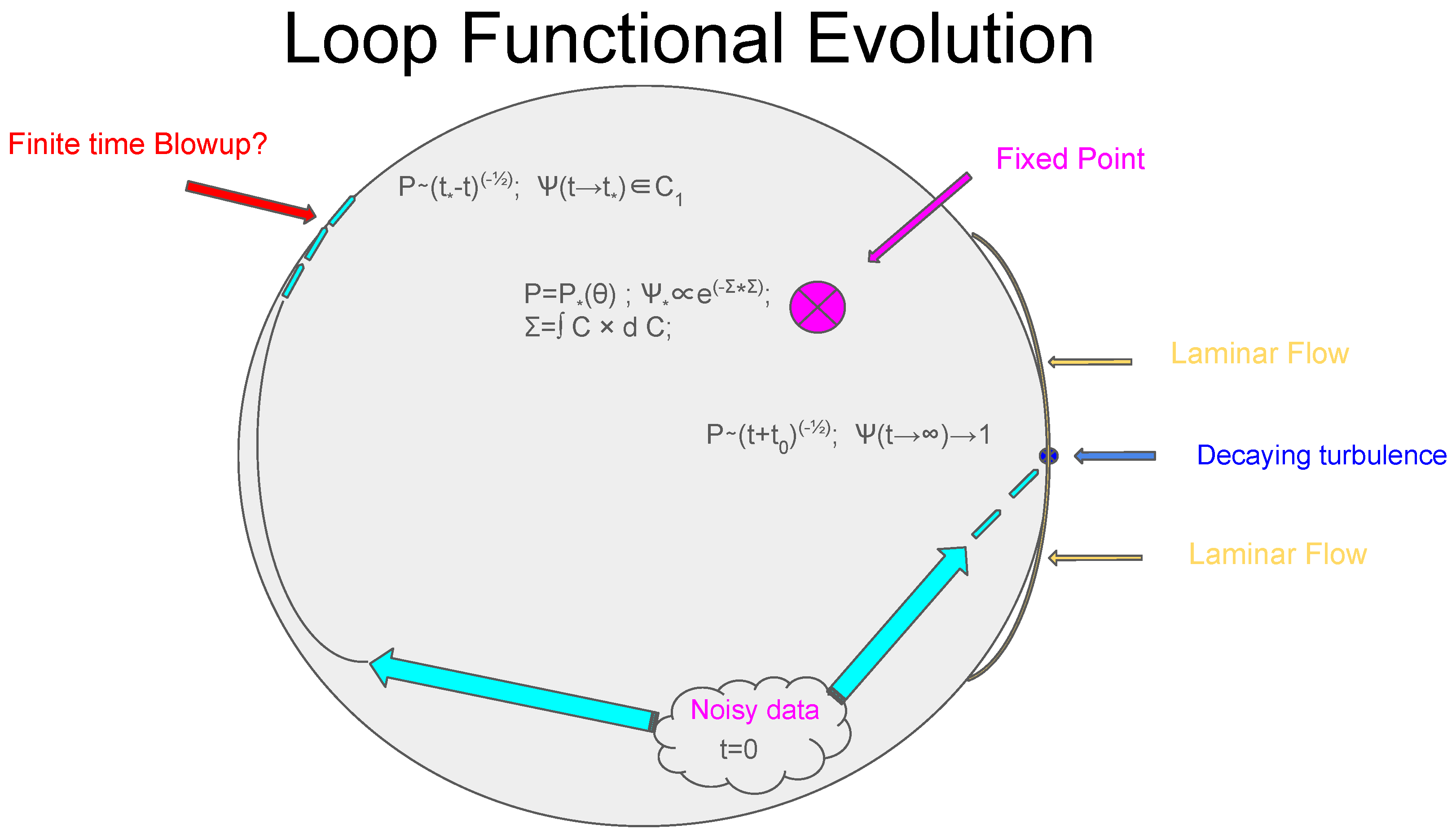
The evolution of the loop functional
inside the unit circle in the complex plane in
Figure 1 goes by universal trajectories, determined by (79). The Reynolds number describes the initial position of this
inside the circle. The distance
from the fixed point
is the true measure of turbulence. One could expect a laminar flow solution in some small vicinity of this fixed point (corresponding to potential flow).
10. Vorticity Statistics and Momentum Loop
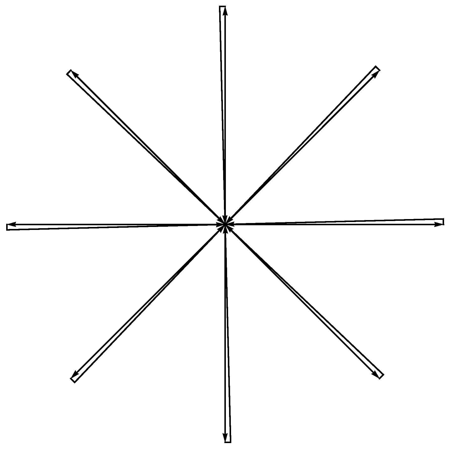
The multiple area derivatives of
yield the formula
where
is a double line from the center of mass,
, to each point
and back to
. The entire loop
C resembles bicycle spokes without a wheel (see
Figure 3). The angles
are ordered on the unit circle.
These double lines cancel in the circulation,
but not in the momentum loop representation. This occurs because, in the momentum loop integral
the momentum variable
depends explicitly on
, preventing the cancellation of the two line integrals in a double line.
The factor
arises as follows. In the velocity representation, where the circulation is zero, the vorticities
depend directly on
, rather than on the angles
. Consequently, the integral over ordered angles
yields the factor
, which we must compensate with the inverse factor.
This leads to the fundamental formula for multiple vorticity correlation functions:
This formula expresses the multiple correlation functions in terms of expectation values within the Euler ensemble. In [
4], we use this approach to compute the two-point correlation function,
, as a function of relative distance for
. The Fourier-space correlation function,
(i.e., the energy spectrum), is found to be real and positive.
We conclude that the full statistical description of the rotational part of the velocity field (i.e., vorticity) is related to the statistics of the solutions of the MLE.
A crucial aspect of this relation is the violation of time-reversal symmetry. Under time reversal, vorticity changes sign, which would typically eliminate vorticity correlations for an odd number of points (n). However, this is not the case in the momentum loop representation (89).
To see why, consider the complex conjugation of the loop functional, which corresponds to time reversal in the original velocity representation. The vorticity operator
in (
84) contains an imaginary unit, so it changes sign. The
P-circulation term in the exponential is real but changes sign under the coordinate reversal
, thereby compensating for the complex conjugation effect.
This results in the identity
which reflects parity conservation but does not enforce time-reversal symmetry. As a consequence, the expectation value of an odd number of vorticities remains an odd function of the coordinates.
More precisely, in both even and odd cases, the expectation values remain real, but they are linked to the real and imaginary parts of the exponential, depending on the number of imaginary units (ı) in the product of vorticities:
11. Laminar Flow at Small Time and Seeds of Turbulence
The viscosity enters the MLE’s denominator, making it straightforward to investigate the laminar flow (large viscosity) and even turbulent flow (small viscosity).
Let us start with the laminar flow. It corresponds to small
, in which case the equation (79) linearizes and can be explicitly solved
This solution will stay smooth when starting with the smooth initial value
. There will be no discontinuity in
and no discontinuity in
.
For the loop functional this means zero area derivative, in other words, potential flow without vorticity. Moreover, this flow will stay as a potential flow in every order of the formal perturbation expansion in inverse powers of for an arbitrary smooth initial value .
However, any finite initial discontinuity in would lead to nontrivial terms of this perturbation expansion. These terms will be singular but scale as higher powers of . One may expect these corrections to be controlled at a large enough viscosity (compared to initial circulation).
The above thermal fluctuations lead to a small but singular contribution to the initial momentum loop. The Fourier coefficients do not decrease with order n, leading to the delta function singularity in the correlation function , which is stronger than the discontinuity, required for the presence of vorticity.
After sufficient time, these small singular terms may lead to larger singular terms in the solution.
The recent paper [
7] argued that the thermal fluctuations could produce turbulence in finite time, comparable with experimental times of the large eddy formation. In other words, these small fluctuations could quickly grow and end up as large random eddies observable in experiments by order of magnitude estimates in [
7].
Our theory considers two possible asymptotic regimes: decaying turbulence or a finite-time explosion. We study these regimes in the subsequent sections.
12. Decaying Turbulence
The solutions originating deep inside the unit circle, far from
, can become turbulent and eventually decay to
due to energy dissipation by vorticity structures. This decay for
corresponds to the fixed point equation for
This fixed point
is not a solution of the Cauchy problem for the loop functional, though we expect the solution of some Cauchy problems to asymptotically approach this fixed point at a large time.
This fixed point represents the solution of the loop equation
with the boundary condition . This boundary condition describes the flow eventually stopping as a result of the dissipation of kinetic energy
12.1. Fixed Point Solution
The saddle point equation (97) was solved and investigated in previous papers [
3,
4]. The solution for
is a fractal curve defined as a limit
of the polygon
with the following vertices
The parameters
are random, making this solution for
a fixed manifold rather than a fixed point. We suggested in [
3] calling this manifold the big Euler ensemble of just the Euler ensemble.
It is a fixed point of (97) with the discrete version of discontinuity and principal value:
Both terms of the right side (79) vanish; the coefficient in front of
and the one in front of
are both equal zero. Otherwise, we would have
, leading to zero vorticity [
3].
This requirement leads to two scalar equations
The integer numbers came as the solution of the loop equation, and the requirement of the rational came from the periodicity requirement, as we prove below.
In our limit, the integral for velocity circulation becomes the Lebesque sum:
A remarkable property of this solution of the loop equation is that even though it satisfies the complex equation and has an imaginary part, the resulting circulation (105) is real! The imaginary part of the does not depend on k and thus drops from the total sum due to the periodicity of the loop C.
Another noteworthy observation is that the solution (
98) exhibits a symmetric distribution:
and
share the same PDF due to integration over all possible rotation matrices. A rotation by
in the
plane, combined with complex conjugation, leaves the distribution invariant. Moreover, as we have seen, the imaginary part of
does not contribute to the loop functional. Consequently, the PDF of
is an even function.
However, multiple vorticity correlations are determined via the area derivative. The corresponding vector in (31d) is quadratic in , and as a result, this reflection symmetry does not suppress the expectation value of an odd number of factors. For instance, the triple correlator remains nonzero. The corresponding triple velocity correlator, , can be obtained via Fourier transformation, where , up to purely potential terms linear in the coordinates.
These potential terms, however, do not contribute to the energy flow in wavevector space, contrary to popular belief, as discussed in [
4]. Instead, they generate gradients of the delta function,
, rather than a constant energy flux. Such terms are influenced by boundary conditions at infinity and, therefore, do not represent spontaneous stochasticity caused by random vortex structures within the bulk.
12.2. The Proof of the Euler Ensemble as a Fixed Point of MLE
Let us present here the proof of this solution, verified by
Mathematica® (see [
8]).
Theorem 1. The Euler ensemble solves the discrete MLE.
Proof. We start from the general Anzatz with real vectors
, corresponding to the real circulation in (105)
Analyzing the imaginary and parts of the second equation in (104), we observe that the imaginary part will vanish provided
We conclude that
belongs to a circle with some radius
R in the origin of the plane, which plane is orthogonal to
. In the coordinate frame where
The
matrix needed to rotate our vectors to this coordinate frame can be absorbed into the rotation matrix
we have in our solution.
The radius
R and
A are determined by the real part of our equations as follows
Solving these two equations, we find the
variables at every step
The radius
R and the length
are related to this angular step
The periodicity of the sequence
requires the angular step to be a fraction of
, which brings us to the Euler ensemble (
98). □
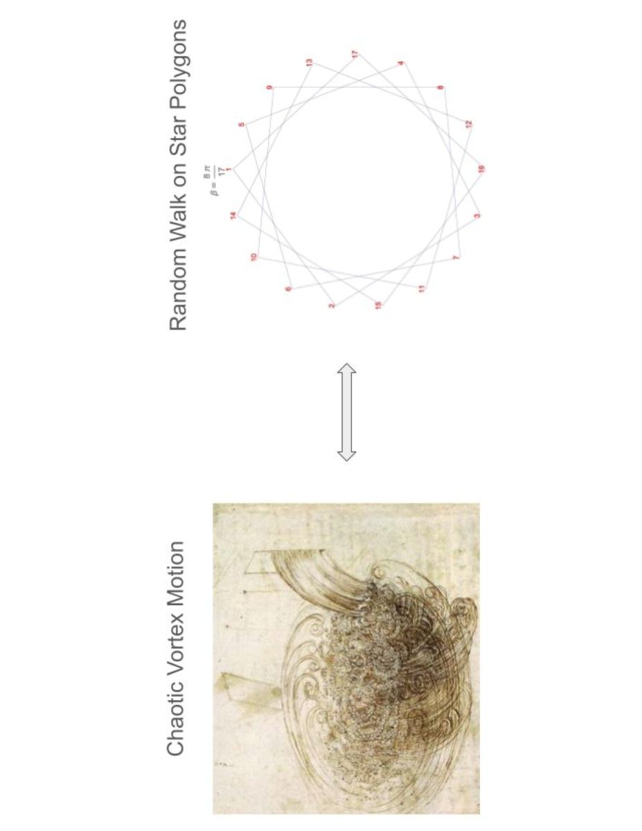
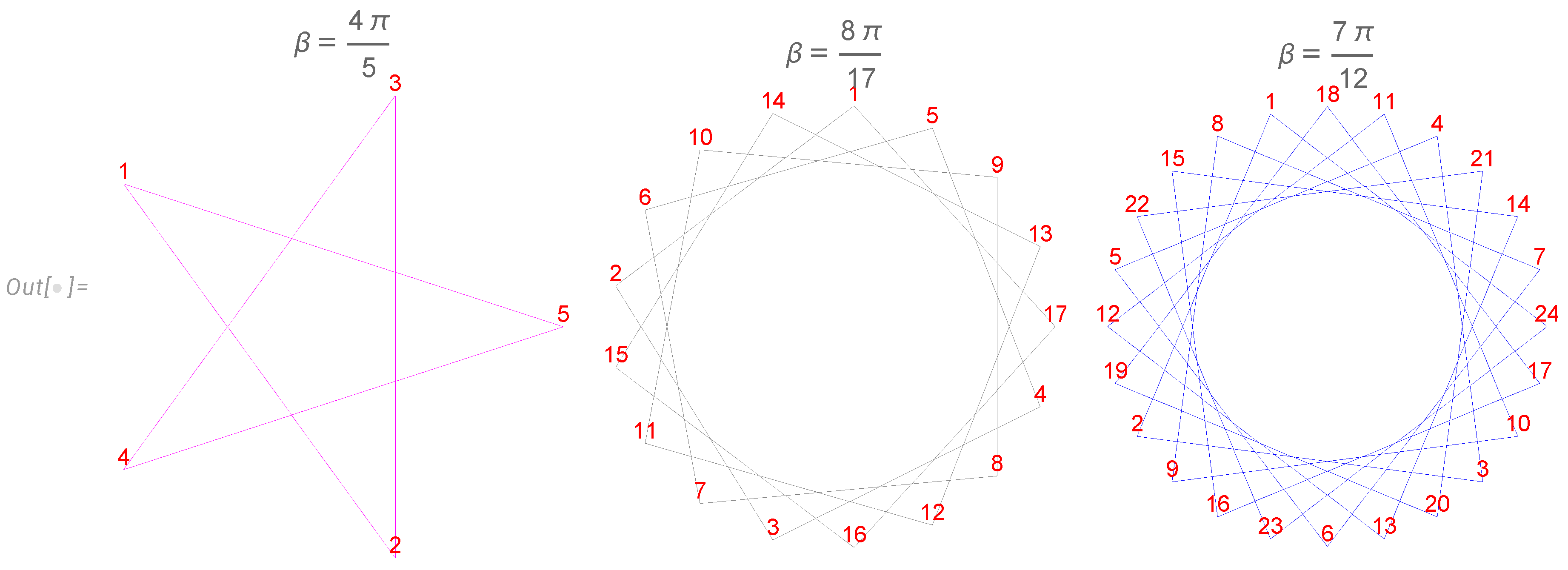
12.3. Euler Ensemble as a Random Walk on a Regular Star Polygon
Geometrically, the vertices belong to the regular star polygon with q sides of unit length, with vertices at . They were classified by Thomas Bradwardine (archbishop of Canterbury) and later by Johannes Kepler in the 17th Century and are denoted as ( so-called Schläfli symbol).
We show several examples in
Figure 4. The general polygon is characterized by co-prime
with
. Euler totients count these polygons. The number
counts the coordinates
covering our polygon several times, so that, in general, each geometric vertex is covered more than once.
The Ising variables describe a random walk around this polygon with the extra condition that it comes to the initial point after N steps. The random walk goes according to the sign of . The periodicity condition requires to be a rational fraction of .
This quantization of the angle and the radius brings the number theory to the statistical distribution. Each polygon may be covered several times during this random walk with this periodicity condition. A certain winding number w is related to . Surprisingly, such a fundamental random walk problem on the 500-year-old geometric manifold has been solved only now.
12.4. Euler Ensemble as String Theory with Discrete Target Space
This random walk problem can also be interpreted as a closed fermionic string in the discrete target space consisting of regular star polygons on a (randomly rotated) plane. Integrating over fermionic degrees of freedom in a quantum trace of the evolution operator is equivalent to summation over occupation numbers , providing directions of the random walk.
The target space coordinates are the vertices of the regular star polygons .
The integration over target space made of these regular star polygons becomes a discrete sum over states of the Euler ensemble: the fraction , the configurations of fermionic occupation numbers and the winding number .
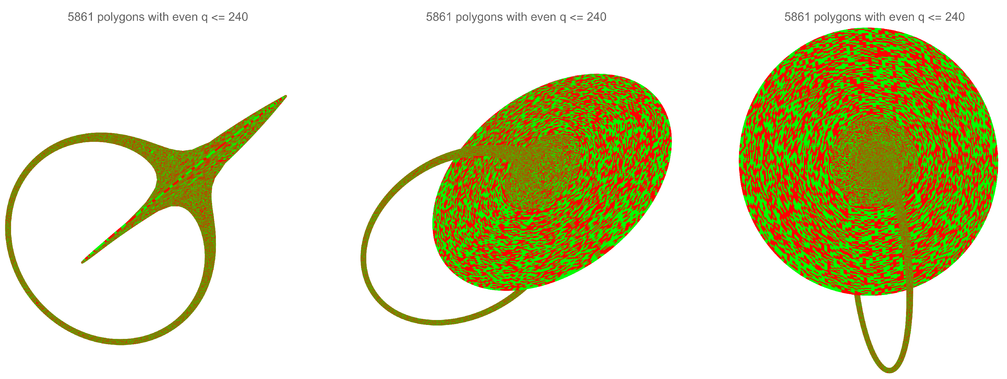
Placing these polygons for a fixed
N on a torus in 3D space ordered by the angle
shows the world sheet of our discrete string in
Figure 5, with red/green colors of sides indicating random directions of random walk (occupation number of fermions). The large disk (infinite at
) corresponds to endpoints
.
The solution of the Euler ensemble[
3] is based on new number theory identities for sums of powers of cotangent of fractions of
. These identities relate these sums to Jordan multi-totient functions weighted with Bernoulli coefficients.
The nontrivial part of using the Euler ensemble is the formula (
82) relating this ensemble to the observable loop functional of the decaying turbulence theory.
In the string theory language, where the momentum loop is the target space along with fermionic occupation numbers, this formula is the dual amplitude for the discrete string theory, with playing the role of external momentum distributed along the closed string position (regular star polygon) .
This turbulence/string duality reveals the hidden beauty of primes under the ugly mask of chaos in the observable turbulent flow.
The corresponding universal energy spectrum for the decaying turbulence was computed in quadrature [
4] in the quasiclassical limit at
, and it closely matched the data of real and numerical experiments. The detailed comparison with available real and numerical experiments in decaying turbulence was published in the previous work [
4,
9]. Let us show here the figures from this work
Figure 6,
Figure 7 demonstrating the match between our theory and the experiments (real and numerical).
12.5. The Limit of Large Reynolds Number Is Not Equivalent to Vanishing Viscosity
The limit
is tricky because
is a measurable physical parameter with dimension
, and it fixes the magnitude of observable quantities. The real limit is the large Reynolds number
where
is a scale of circulation in the problem. Our formula for the dissipation is
Mathematically, the same turbulent limit
can be achieved by tending
, as only the ratio enters the exponential.
This limit will exist in our theory if we balance the powers of
with powers of
to keep the dissipation finite. This requires
as we found in the first paper [
3].
The dimensionless parameters and functions of scaling arguments such as where all stay finite in this limit.
Other observable quantities, such as the energy spectrum or kinetic energy are not initially proportional to which means that the powers of N will not balance in these quantities.
The resolution of this paradox is as follows [
4]. The two-point vorticity correlation function must have a pole in the mathematical limit
to provide finite energy dissipation:
The residue
in this pole is what we call the turbulent limit
We use the mathematical limit
to compute this residue, but after that, we come back to the physical formula (
118) with observable viscosity
and
.
So, we used the fictitious limit of zero viscosity to compute the residue of the observable correlator at zero viscosity.
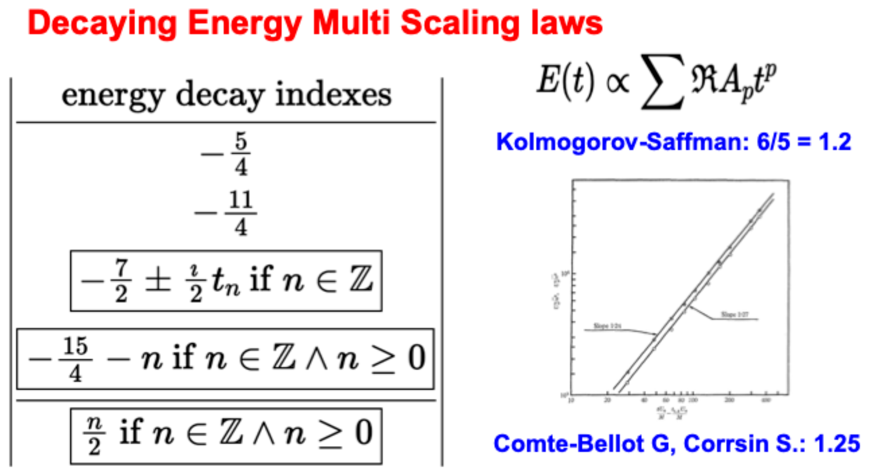
12.6. Continuum Limit Exists for the Loop Functional But Not for the Momentum Loop
There is a following peculiarity in our theory. The momentum loop has no continuum limit when , but the original loop functional stays finite in such a limit. To be more precise, there is renormalizability: the energy dissipation stays finite when .
The second moment of velocity difference
as a function of scaling variable
decays at small argument as an infinite series of power terms with growing positive powers
. The spectrum of these scaling indexes
p (unrelated to a dilatation operator as far as we know) is given in the following table:
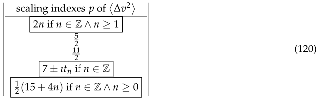
Here are imaginary parts of the zeros of , all located at the ray , according to the Riemann hypothesis. At least, it was proven that these zeros are all inside the strip .
The second moment does not scale as a single power. The effective index (log derivative of the second moment as a function of coordinate difference), is a nontrivial function of the scaling variable
. The DNS data from two numerical simulations of the NS equation is shown as red and blue dots with error bars in
Figure 7, together with our theory (green curve) and the Kolmogorov
prediction (black dashed line).
Our theory matches the data within a few % margin of error. The Kolmogorov scaling is totally off the charts. The data index crosses the K41 value without any inertial range (the effective index plot is supposed to show a plateau around
in the K41 model). Thus, there is no cascade in decaying turbulence (see [
4] for a discussion of this issue).
Our solution has a well-defined continuum limit for observable variables such as decaying kinetic energy, energy spectrum, and moments of velocity difference, closely matching experiments.
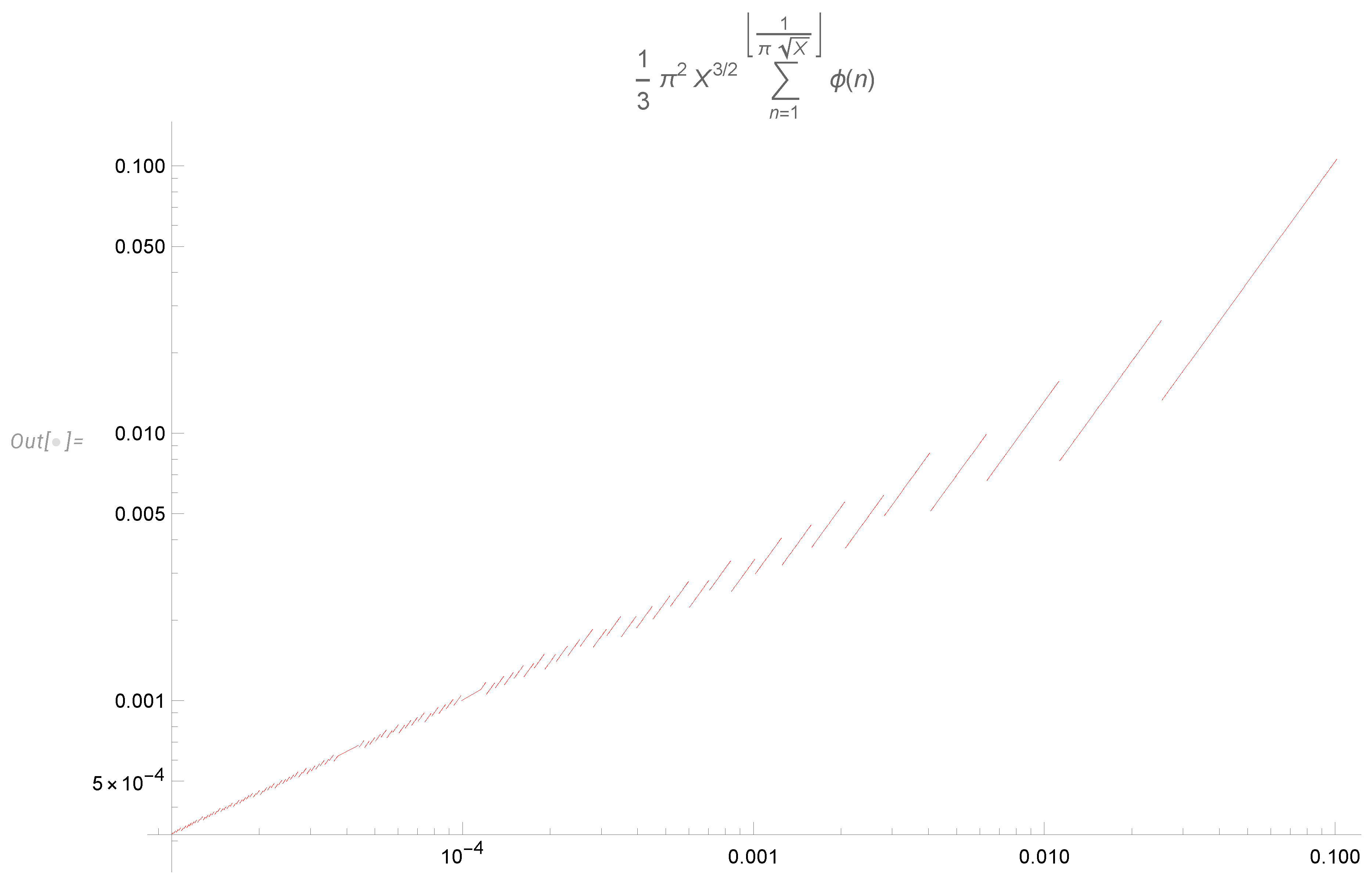
At the same time, the dual system– the string itself– does not have any continuum limit. The regular star polygons with unit side have the radia
, which vary between
and
∞ but do not converge to any continuous function, with
being co-prime numbers. The distribution of the variable
for large co-prime
was studied in the previous work, and it is a discontinuous piecewise power like distribution
depicted in
Figure 8. Here
is the totient summatory function
This manifests the same phenomena we observed in the simplest solvable case of constant global rotation. This stationary solution of the NS equation studied in the
Section 7 at finite
N is a finite sum of Gaussian random variables. However, there is no limit
in this sum. Only the loop functional, related to the variance of the random variable
tends to a finite limit related to the tensor area
.
In our solution of decaying turbulence, there are no random Gaussian variables: there’s a random walk on random regular star polygons, equivalent to a string theory with discrete target space, which does not possess any continuum limit. At the same time, the dual amplitudes of this string theory have a continuum limit, providing the solution for the loop functional.
12.7. An Open Problem of the Stability of Euler Ensemble as MLE Fixed Point
The interesting and unexpected property of the Euler ensemble solution of the MLE is its independence of the spectral parameter . The dependence reappears in the linearized MLE for the small deviations from the fixed point. These deviations describe the approach of the solution of the MLE to the fixed trajectory of decaying turbulence.
As we found in the first paper [
3], these deviations decay by power laws with some indexes, depending on
The spectral equation for these decay indexes
was written down in [
3] for the finite
N in the Euler ensemble. The problem of the continuum limit of this spectrum is yet to be solved.
13. Inconsistency of explosive solution
Within our dual theory, there is, in principle, a possibility for finite-time explosion with at some finite moment .
In that case, only the third-degree terms will remain on the right side, with the linear term becoming negligible at
. The scale invariance fixes the time dependence in this case, so the solution becomes
We assume that the trajectory of singularity
is a continuous function of
or a constant. In this case, all the terms on the right of the equation (97) have a common time dependence
, matching the left side. The vector function
must satisfy the following equation:
The left side of this equation for
differs from the left side of the equation (97) for the fixed point for
.
The following theorem proves the lack of a solution for this fixed point .
Theorem 2.
There is no explosive solution to the MLE with singularity position being a continuous function of the angle
.
Proof. Let us assume such a solution with some vector function and arrive at a contradiction. This vector equation is a linear combination of two vectors . Both coefficients must be zero. Otherwise, these two vectors are parallel, or else one of them vanishes. In both cases, the vorticity at the loop vanishes at every point on the unit circle. Without vorticity, the solution reduces to the trivial fixed point .
Now, the first coefficient a can only vanish if has some imaginary component, which contradicts the requirement that the circulation is a real variable.
This requirement allows for a constant imaginary term in , as this continuous term will drop in the closed loop integral. This requirement implies real discontinuity . In the explosion equation (124) with , there is no real solution with . □
We have proven the inconsistency of the finite-time explosion in the momentum loop dynamics, i.e., the Navier-Stokes dynamics with noisy initial data and constant or vanishing velocity at infinity.
This inconsistency is a consequence of the universality and dimensional reduction of the dual fluid dynamics, leading to much more stringent conditions on a potential explosion solution, which we have proven inconsistent.
In the conventional approach to the Navier-Stokes equation, without the noise in initial data, Constantin and Fefferman have proven a theorem about the solution’s regularity [
10]. As a consequence of this theorem, any singular solution must have vorticity growing to infinity at some point in time in some region in space.
In the MLE equation, vorticity at the loop would have a finite time singularity with the above hypothetical solution
In particular, the mean square of vorticity (so-called enstrophy) would have a double pole
The growth of vorticity was proven necessary for the singular solution of Navier-Stokes equation in [
10], and in our theory, it is ruled out.
If proven to stay in the smooth limit
, without extra condition of continuous
this proof would provide a negative answer to the notorious problem of the explosion in the Navier-Stokes equation, leaving two remaining alternatives: smooth (laminar) solution and a stochastic (turbulent) solution which we have found before [
3,
4] and reinterpreted in this work as a string theory.
Presumably, decaying turbulence occurs at a large enough Reynolds number in the initial data; otherwise, the solution stays smooth.
14. Discussion
The discovery of a new connection between different branches of science often lays the groundwork for unifying theories. Here, we outline potential generalizations of our findings on the equivalence between Navier-Stokes (NS) turbulence and random walks on discrete manifolds. These extensions open exciting directions for both physical applications and mathematical exploration.
14.1. Physical Generalizations
The applicability of the loop equations extends to other nonlinear systems that exhibit turbulence or finite-time singularities. Below, we propose several potential extensions, organized by increasing complexity:
Forced turbulence driven by random rotations. In this analytically solvable case, the loop equations, modified to include random centrifugal forces, exhibit a fixed point describing the steady state of forced turbulence with energy flow [
11].
Compressible fluids. Adapting the framework to compressible flows requires replacing the incompressibility condition with variable-density dynamics, governed by the conservation of the volume element.
Magnetohydrodynamics (MHD). In MHD, the circulation variables naturally split into two components encircling vorticity and magnetic fluxes. This generalization produces richer loop equations and leads to new insights into turbulence in plasmas. Preliminary analysis [
12] reduces the solution of MHD turbulence to the synchronized random walks on two regular star polygons.
Passive scalars. The advection of passive scalar fields in a turbulent flow can be expressed via path integrals involving the loop functional. These integrals suggest analogies with gauge theories, offering new perspectives on scalar turbulence statistics.
General relativity. Could turbulence mechanisms regularize naked singularities in Einstein’s equations? While speculative, we propose studying the classical Einstein loop equations for stochastic effects. Analogous to the NS case, such stochastic mechanisms may provide an alternative to singularities, hinting at deeper connections between fluid dynamics and gravity.
14.2. Mathematical Directions
In addition to physical extensions, our framework suggests new mathematical avenues:
Classification of dual PDEs. Identifying classes of partial differential equations (PDEs) with dualities to quantum mechanical systems in loop space could deepen our understanding of nonlinear systems.
Dimensional reduction. Exploring which dual PDEs can be reduced to one-dimensional nonlinear momentum loop equations may simplify otherwise intractable problems while preserving essential dynamics.
Nonlinear spaces. Generalizing the observed random walks on star polygons to loop groups and other nonlinear spaces may reveal new connections between geometry, number theory, and fluid mechanics.
Summing over topologies? The turbulent flows can exist (at least mathematically) in spaces of arbitrary topology, for example, on a manifold of higher genus. The natural generalization of the discrete string theory made of regular star polygons also allows topological transition when a polygon with a winding number n bifurcates into two polygons with winding numbers , which later evolve the same way as before. The opposite process of merging is also possible without breaking any features of preceding or subsequent propagation. How to sum our WKB solution of the Euler ensemble over topologies? How are they related to decaying turbulence in "physical" space?
15. Conclusion
This work has demonstrated a duality between classical incompressible fluid mechanics in Euclidean space and nonlinear dynamics in loop space. By reformulating the Navier-Stokes equations in terms of loop dynamics, we uncover universal properties of turbulent flows, providing new insights into the structure of decaying turbulence. Key contributions of this study include:
The classical Navier-Stokes equations, when supplemented by thermal fluctuations, can be reformulated as a dimensional equation (79) for the momentum loop trajectory . The loop functional (97) is related to the momentum loop via equation (82), providing a direct connection between turbulence and loop dynamics.
The viscosity vanishes from the momentum loop equation (79), rendering the momentum loop trajectories completely universal. In this framework, the Reynolds number becomes a property of the initial data , corresponding to a stochastic loop in .
A degenerate fixed point,
, is associated with the decaying turbulence solution. This fixed point corresponds to a periodic random walk on a regular star polygon with
steps. It is analytically characterized by the Euler ensemble, as described in previous works [
3,
4]. The energy spectrum of this fixed point has been computed in quadrature and validated against experimental data.
The Euler ensemble is equivalent to a string theory with a target space composed of regular star polygons. This solvable string theory provides an explicit example of a decaying stochastic solution to the unforced Navier-Stokes equation, bridging classical turbulence and quantum-inspired mathematical structures.
While we have not proven that this solution is reachable from smooth initial data (corresponding to vanishing noise, , or ), the presence of thermal noise in physical fluids ensures the relevance of this solution in realistic scenarios. This highlights the idealized nature of the conventional Cauchy problem, which assumes perfect smoothness of initial conditions.
We have established a
No Explosion Theorem, ruling out finite-time blow-ups for arbitrary initial data with finite noise. This result leaves only two viable alternatives: the well-known smooth laminar solutions and the decaying turbulence solution (Euler ensemble = discrete string theory) [
3,
4].
The insights presented in this work suggest that turbulent flows, despite their apparent randomness, may be governed by universal principles encoded in the geometry of loop space. By connecting turbulence to discrete geometry and solvable string theories, we provide a foundation for new approaches to understanding turbulence across scales. This framework has implications not only for fluid mechanics but also for broader applications in mathematical physics, including magnetohydrodynamics, compressible flows, and flows in nonlinear spaces.
Acknowledgments
I benefitted from discussions of this work with Camillo de Lellis, Elia Bruè, Stan Palasek, Semon Rezchikov and Jincheng Yang. The most valuable advice came from Albert Schwartz. This research was supported by the Simons Foundation award ID SFI-MPS-T-MPS-00010544 in the Institute for Advanced Study.
Appendix A Momentum Loop Distribution for Noisy Velocity
In the polygonal approximation, the path integral (59) becomes a multiple Fourier integral
We rewrite it as a multiple integral over steps
Introducing a Fourier integral for the delta function we find
Now the integral over
is calculable ( I skip positive normalization factors, and use known angular integral
):
Collecting the factors we get a POSITIVE measure
In the limit of large
N this becomes a Gaussian measure
This ensemble assumed fixed
. One can make this
N variable and introduce a weight
(so called canonical ensemble as opposed to a micro-canonical with fixed
N). In that case, in the continuum limit, summation over
N becomes an integral
and we get
with corresponding factors absorbed into
. This is the distribution quoted in the text of the paper.
References
- Migdal, A. Loop Equation and Area Law in Turbulence. In Quantum Field Theory and String Theory; Baulieu, L.; Dotsenko, V.; Kazakov, V.; Windey, P., Eds.; Springer US, 1995; pp. 193–231. [CrossRef]
- Migdal, A. Statistical Equilibrium of Circulating Fluids. Physics Reports 2023, 1011C, 1–117, [arXiv:physics.flu-dyn/2209.12312]. [CrossRef]
- Migdal, A. To the Theory of Decaying Turbulence. Fractal and Fractional 2023, 7, 754, [arXiv:physics.flu-dyn/2304.13719]. [CrossRef]
- Migdal, A. Quantum solution of classical turbulence: Decaying energy spectrum. Physics of Fluids 2024, 36, 095161. [CrossRef]
- Ohkitani, K. Study of the Hopf functional equation for turbulence: Duhamel principle and dynamical scaling. Physical Review E 2020, 101, 013104.
- Polyakov, A.M. Gauge Fields and Strings; Taylor & Francis, 1987.
- Bandak, D.; Mailybaev, A.A.; Eyink, G.L.; Goldenfeld, N. Spontaneous Stochasticity Amplifies Even Thermal Noise to the Largest Scales of Turbulence in a Few Eddy Turnover Times. Physical Review Letters 2024, 132. [CrossRef]
- Migdal, A. Decaying Turbulence Computations. https://www.wolframcloud.com/obj/sasha.migdal/Published/DecayingTurbulenceComputations.nb, 2023.
- Migdal, A. Hierarchical Structure of Quantum Solution. https://sashamigdal.github.io/QuantumSolution/, 2024.
- Constantin, P.; Fefferman, C. Direction of Vorticity and the Problem of Global Regularity for the Navier-Stokes Equations. Indiana University Mathematics Journal 1993, 42, 775–789. [CrossRef]
- Migdal, A. Quantum Solution of Classical TurbulenceForced by Random Rotation, 2025. "In preparation".
- Migdal, A. Duality of the decaying MHD to the Euler ensemble, 2025. "In preparation".
| 1 |
We do not count deterministic fixed points corresponding to potential flows. They correspond to isolated points moving on the unit circle. |
Figure 1.
Asymptotic trajectories of the time evolution for the loop functional inside the unit circle in the complex plane. The laminar flow is the yellow region on the circle close to . Three other flows are 1) hypothetical explosion, 2) decaying turbulence, and 3) special fixed point.
Figure 1.
Asymptotic trajectories of the time evolution for the loop functional inside the unit circle in the complex plane. The laminar flow is the yellow region on the circle close to . Three other flows are 1) hypothetical explosion, 2) decaying turbulence, and 3) special fixed point.
Figure 2.
The "hairpin" loop C used in defining the pair correlation of vorticity. The little circles are the loop variations needed to bring down vorticity at two points in space. The backtracking contribution to the circulation cancels at vanishing separation between these parallel lines.
Figure 2.
The "hairpin" loop C used in defining the pair correlation of vorticity. The little circles are the loop variations needed to bring down vorticity at two points in space. The backtracking contribution to the circulation cancels at vanishing separation between these parallel lines.
Figure 3.
The loop C used to compute vorticity correlation functions. The endpoints of each spoke correspond to , while the center represents the center of mass, . Each spoke consists of two segments: one from the center to , and another returning to the center. Since the area enclosed by the loop is zero, the circulation vanishes, i.e., .
Figure 4.
regular star polygons for Euler ensembles of various . The variable indicates the direction of the random step of the link . The random walk could go several times around the polygon as long as it ends where it started.
Figure 4.
regular star polygons for Euler ensembles of various . The variable indicates the direction of the random step of the link . The random walk could go several times around the polygon as long as it ends where it started.
Figure 5.
The world sheet of our discrete string made of regular star polygons with unit side. The red/green colors of the sides indicate random directions of random walk.
Figure 5.
The world sheet of our discrete string made of regular star polygons with unit side. The red/green colors of the sides indicate random directions of random walk.
Figure 6.
The predictions of this theory compared with grid turbulence decay data from 1966. This data significantly deviate from Kolmogorov-Saffman model prediction but perfectly matches the leading decay index predicted by our theory.
Figure 6.
The predictions of this theory compared with grid turbulence decay data from 1966. This data significantly deviate from Kolmogorov-Saffman model prediction but perfectly matches the leading decay index predicted by our theory.
Figure 7.
We used the raw data from the new DNS by A. Rodhiya and K.R. Sreenivasan (lattice ) and the older one by J.J Panicacheril, D. Donzis, and K.R.Sreenivassan (lattice ). In the lower-left corner, the effective index for the second moment of velocity is plotted as a function of in the turbulent range. Both data sets perfectly match the theoretical curve (green line) within the error bars. We only display the larger set results, which extend to lower values of the index, below 0.5. The errors are small in the upper part of the curve(above 0.5) and rapidly grow below that value, as it corresponds to large coordinate scales, where the lattice artifacts dominate. Both matching curves theory/DNS deviate very far from the prediction of the K41 model . On the upper left, the effective length is compared with our prediction in the form of inverse function . It matches well in a wide time interval, which we interpret as decaying turbulence range. On the right side, there are two plots comparing decaying energy with the predictions (green) and the simple power law for the two DNS data. There is a perfect match in the turbulent time range.
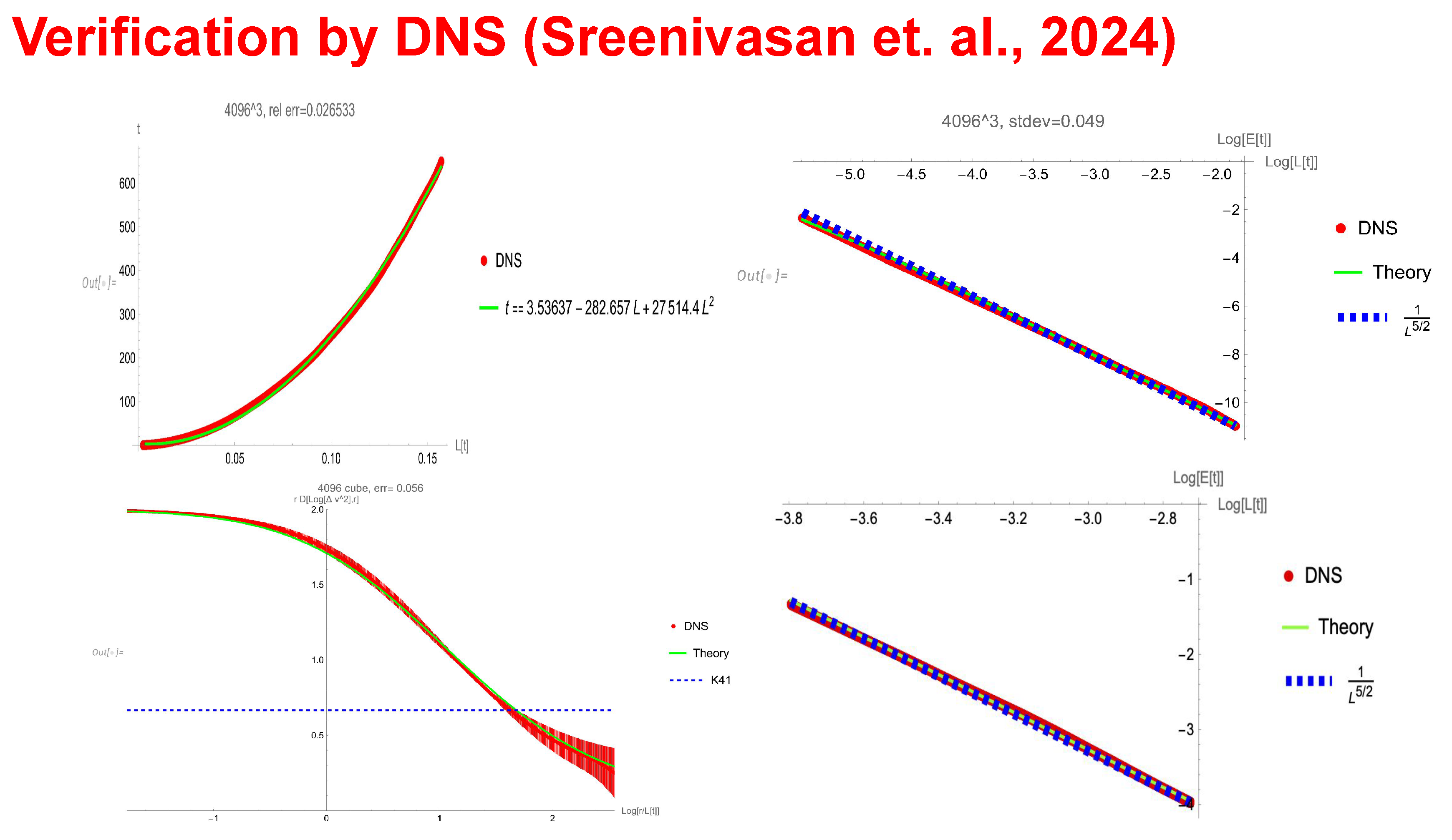
Figure 8.
Log log plot of the distribution (121)
Figure 8.
Log log plot of the distribution (121)
|
Disclaimer/Publisher’s Note: The statements, opinions and data contained in all publications are solely those of the individual author(s) and contributor(s) and not of MDPI and/or the editor(s). MDPI and/or the editor(s) disclaim responsibility for any injury to people or property resulting from any ideas, methods, instructions or products referred to in the content. |
© 2025 by the authors. Licensee MDPI, Basel, Switzerland. This article is an open access article distributed under the terms and conditions of the Creative Commons Attribution (CC BY) license (http://creativecommons.org/licenses/by/4.0/).