The Logic of Fluids: Coherence and Regularity in the Navier–Stokes System

1. Introduction: Regularity as Structural Necessity

This manuscript presents a structural proof of global regularity for the three-dimensional incompressible Navier–Stokes equations on ${\mathbb{R}}^3$.

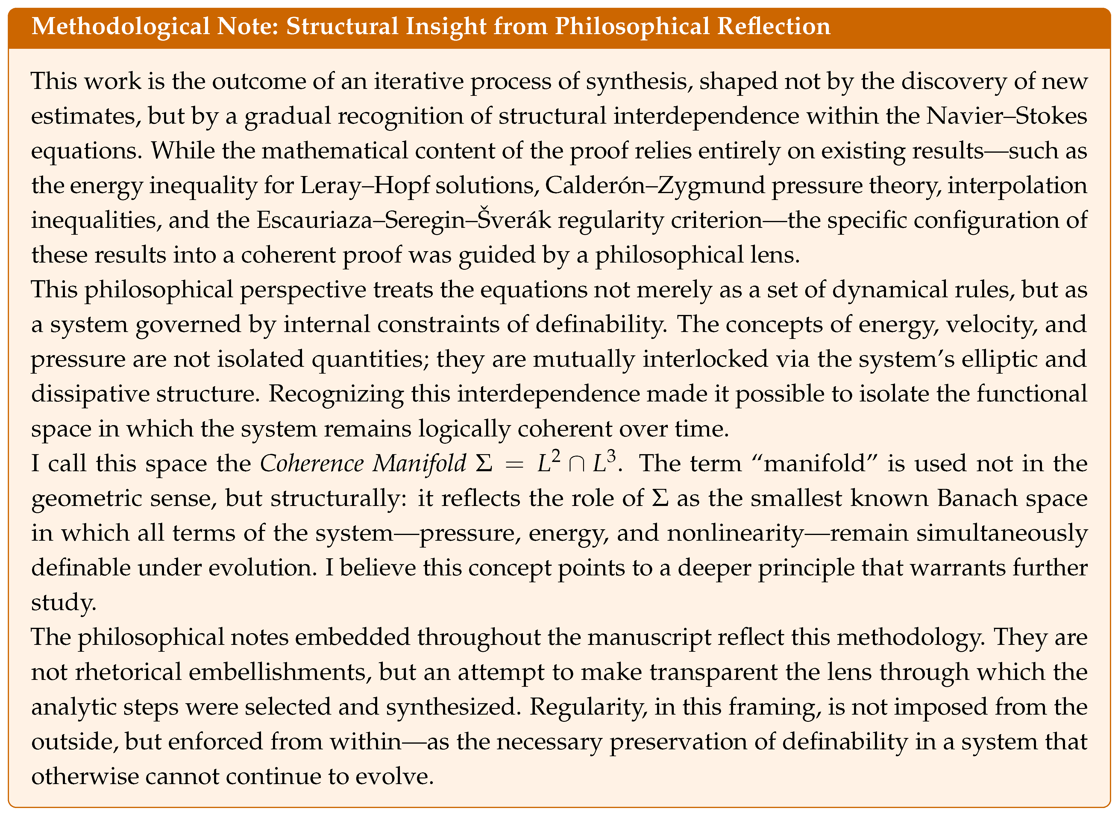
Unlike analytic approaches that aim to control singularities by bounding critical norms, we show that the system’s own internal grammar prevents incoherence. The Navier–Stokes equations form a tightly coupled triad: pressure enforces incompressibility through elliptic constraint, velocity evolves dynamically, and energy dissipates irreversibly. These components are logically interlocked — none can be defined without the others.

To make this idea precise, we introduce the Coherence Manifold1

$$\mathrm{\Sigma }:=\left\{u\in L^2\left({\mathbb{R}}^3\right)\cap L^3\left({\mathbb{R}}^3\right)|\nabla ·u=0\right\},$$

the minimal space in which all terms of the Navier–Stokes system remain mathematically well-defined:

• the $L^2$ norm ensures finite energy,
• the $L^3$ norm aligns with the system’s critical scaling and ensures pressure definability,
• and the nonlinearity $(u·\nabla )u$ is distributionally meaningful.

We show that the system’s own structure enforces persistence in $\mathrm{\Sigma }$. If a solution begins in this space, it cannot exit without violating the energy inequality or the pressure constraint. This internal rigidity — not any external bound — precludes the formation of singularities.

This reframes the Clay Millennium Problem [1], which asks:

• Given smooth, divergence-free initial data $u_0\in C_c^{\infty }\left({\mathbb{R}}^3\right)$, does there exist a unique, smooth solution $u(x,t)$ for all $t>0$?

Rather than attempting to suppress blow-up, we show that the system forbids it — because a blow-up would constitute a collapse of definability, and therefore a contradiction.

The structure of the argument is as follows:

• Section 2 derives the pressure equation and structural triad.
• Section 3 formalizes $\mathrm{\Sigma }$ and proves that solutions cannot leave it.
• Section 4 invokes the Escauriaza–Seregin–Šverák theorem to conclude regularity.
• Section 5 applies this framework to resolve the Clay problem.
• Section 6 reflects on the implications of coherence as a structural law.

2. The Structural Grammar of Flow

This section analyzes the internal structure of the incompressible Navier–Stokes equations in ${\mathbb{R}}^3$, with the goal of identifying the minimal functional requirements for the system to remain logically coherent.

We examine how the pressure field is determined by the velocity through elliptic structure, how the energy inequality imposes an irreversible dissipation law, and how the nonlinear term $(u·\nabla )u$ depends on the integrability of u to remain distributionally defined.

Together, these interdependencies form a self-referential triadic system:

• The  velocity  evolves dynamically,
• The  pressure  enforces incompressibility through elliptic constraint,
• The  energy  decays in accordance with dissipation.

These components are not analytically independent — they are logically coupled. This section makes that coupling explicit, preparing the way to define a functional space in which this structural coherence is preserved. In the next section, we formalize that space as the Coherence Manifold.

2.1. Rewriting the Equations

We begin with the incompressible Navier–Stokes equations in ${\mathbb{R}}^3$:

$$\begin{array}{cc}\hfill {𝜕}_{t}u+(u·\nabla )u& =-\nabla p+\nu \Delta u,\hfill \end{array}$$

(1)

$$\begin{array}{cc}\hfill \nabla ·u& =0.\hfill \end{array}$$

(2)

Our objective is to understand the role of pressure $p(x,t)$, which appears not to have its own evolution equation. Instead, it is entirely dictated by the velocity field u in a way that ensures incompressibility (2).

2.2. Taking the Divergence

We compute each term individually to isolate the structure of the pressure equation:

$$\nabla ·\left({𝜕}_{t}u+(u·\nabla )u\right)=\nabla ·\left(-\nabla p+\nu \Delta u\right).$$

1.

Divergence of ${𝜕}_{t}u$

Since time derivative and divergence commute:

$$\nabla ·\left({𝜕}_{t}u\right)={𝜕}_t(\nabla ·u)={𝜕}_t\left(0\right)=0.$$

2.

Divergence of the nonlinearity

In components:

$$\nabla ·\left((u·\nabla )u\right)={𝜕}_i\left(u_j{𝜕}_j{u}_i\right)=\left({𝜕}_i{u}_j\right)\left({𝜕}_j{u}_i\right)+u_j{𝜕}_i{𝜕}_j{u}_i.$$

3.

Divergence of pressure gradient

$$\nabla ·(-\nabla p)=-\Delta p.$$

4.

Divergence of viscous term

$$\nabla ·(\nu \Delta u)=\nu \Delta (\nabla ·u)=0.$$

Putting everything together:

$$\nabla ·\left(\right(u·\nabla \left)u\right)=-\Delta p,$$

which yields the pressure Poisson equation:

$$\begin{array}{|c|}\hline \Delta p=-\nabla ·\left((u·\nabla )u\right)\\ \hline\end{array}$$

(3)

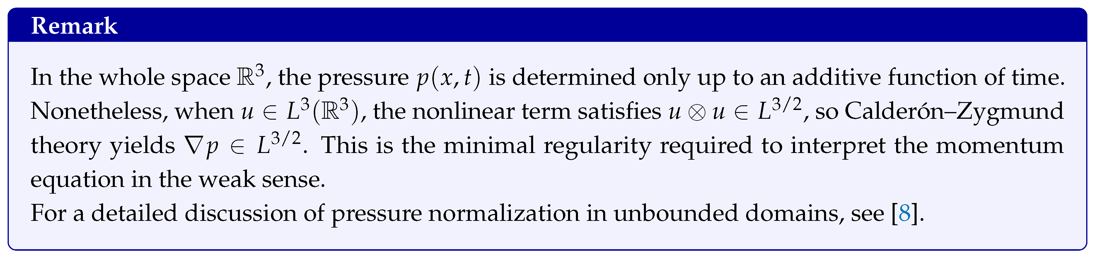
2.3. Tensor Form and Calderón–Zygmund Regularity

If $\nabla ·u=0$, then $(u·\nabla )u=\nabla ·(u\otimes u)$, so the pressure equation becomes:

$$\begin{array}{|c|}\hline \Delta p=-\nabla ·\nabla ·(u\otimes u)\\ \hline\end{array}$$

(4)

The elliptic equation can be formally inverted using Calderón–Zygmund singular integral theory:

$$p\left(x\right)=\sum _{i,j=1}^3{R}_i{R}_j\left(u_i{u}_j\right)\left(x\right),$$

where $R_j$ are the Riesz transforms:

$$R_{j}f\left(x\right)=p.v.{\int }_{{\mathbb{R}}^3}{\displaystyle \frac{x_j-y_j}{{|x-y|}^4}}f\left(y\right)dy{.}^2$$

By Calderón–Zygmund theory (see [4]), we have:

$${\parallel \nabla p\parallel }_{L^q}\lesssim {\parallel u\otimes u\parallel }_{L^q}\lesssim {\parallel u\parallel }_{L^{2q}}^2,\mathrm{for}1<q<\infty .$$

(5)

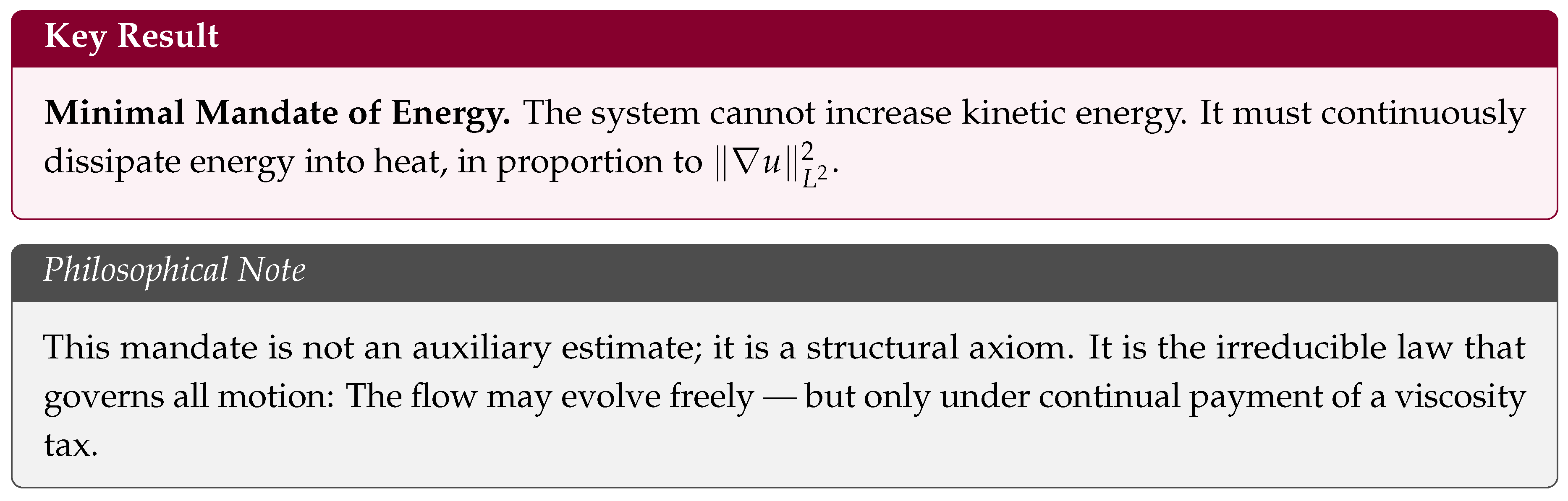
2.4. The Minimal Mandate of Energy

The foundational constraint in the Navier–Stokes system is the energy inequality. For any Leray–Hopf weak solution u, we have:

$${\displaystyle \frac{1}{2}}{\parallel u\left(t\right)\parallel }_{L^2}^2+\nu {\int }_0^t{\parallel \nabla u\left(s\right)\parallel }_{L^2}^{2}ds\le {\displaystyle \frac{1}{2}}{\parallel u_0\parallel }_{L^2}^2.$$

(6)

This implies two critical facts:

• ${\parallel u\left(t\right)\parallel }_{L^2}$ is uniformly bounded for all $t\ge 0$,
• $\nabla u\in L^2([0,T];L^2\left({\mathbb{R}}^3\right))$ for any $T>0$.

This inequality is minimal in the sense that it holds without any assumptions of smoothness, and it defines the lowest-order space in which the Navier–Stokes system admits a meaningful global constraint. The energy space $L^2$, together with the dissipation term $\nabla u\in L^2$, is the only Hilbert space in which the kinetic energy and viscous term are both well-defined and conserved in a distributional sense.

Moreover, this inequality provides the foundation for all further control: when combined with interpolation, it implies that $u\in L_t^3{L}_x^3$, establishing coherence at the critical level. Thus, the energy inequality not only expresses physical dissipation, but also initiates the structural feedback loop that enforces definability.

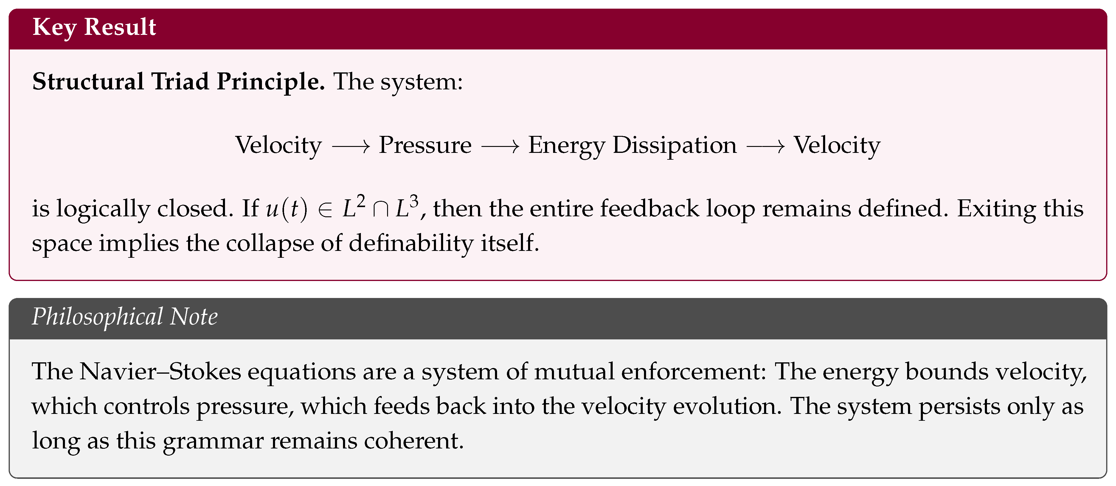
2.5. The Structural Triad: Energy, Velocity, Pressure

We now emphasize the essential interdependence of the three central quantities in the Navier–Stokes system:

• Velocity $u(x,t)$ — the evolving vector field.
• Pressure $p(x,t)$ — an elliptic field ensuring incompressibility.
• Energy $E\left(t\right):={\displaystyle \frac{1}{2}}{\parallel u\left(t\right)\parallel }_{L^2}^2$ — a global invariant under dissipation.

This gives rise to the following logical loop:

1.

$u\in L^2\cap H^1\Rightarrow u\otimes u\in L^{3/2}$

2.

$\Rightarrow \nabla p\in L^{3/2}$ via elliptic theory.

3.

⇒ The nonlinear term $(u·\nabla )u\in L^{3/2}$.

4.

⇒ The weak formulation of the Navier–Stokes equations is well-defined.

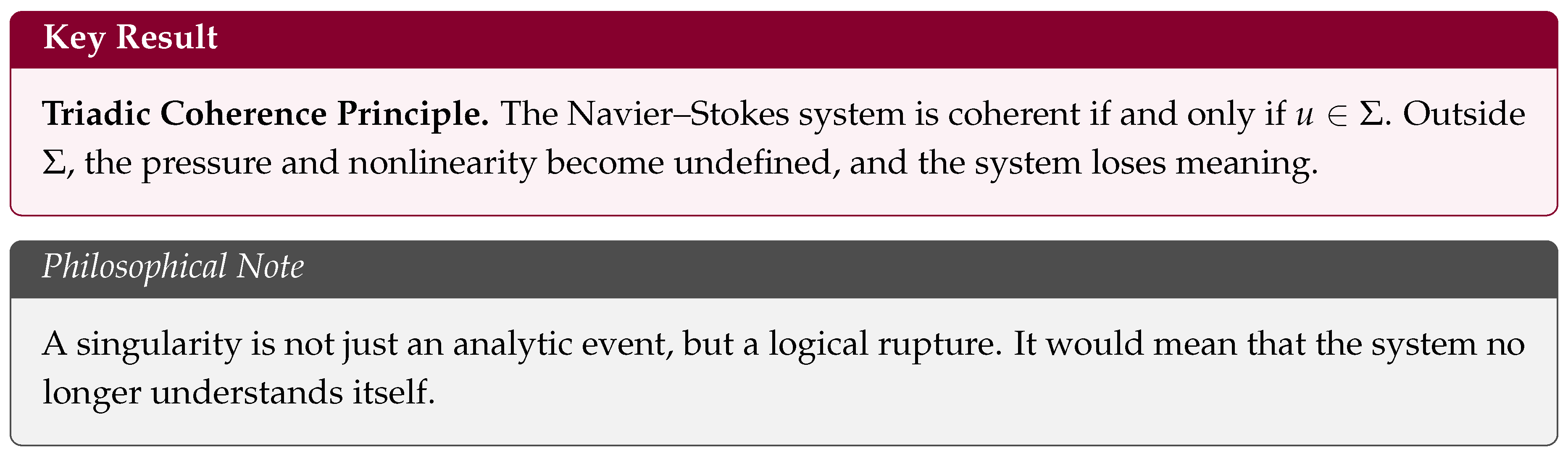
3. The Coherence Manifold

This section formalizes the  Coherence Manifold  $\mathrm{\Sigma }=L^2\cap L^3$, the minimal functional space in which the Navier–Stokes equations remain logically coherent: the velocity, pressure, and energy are mutually definable, and the nonlinear term $(u·\nabla )u$ is valid in the distributional sense.

We show that Σ is not an arbitrary regularity class, but the precise intersection of:

• finite energy ($L^2$),
• critical scaling invariance ($L^3$),
• and pressure coherence via Calderón–Zygmund theory.

From this structure, we prove two key results:

1.

Structural Rigidity: a Leray–Hopf solution starting in Σ cannot exit it — coherence is preserved by the system’s own energy constraints.

2.

Structural Uniqueness: within Σ, the solution is unique — no branching or bifurcation is possible in the space of coherent flows.

These results establish Σ as a structurally invariant and deterministically closed domain. It is not merely a space of control, but a space of definability and uniqueness — within which the Navier–Stokes system becomes fully self-determining.

3.1. Definition of the Coherence Manifold

We define the Coherence Manifold as

$$\mathrm{\Sigma }:=\left\{u\in L^2\left({\mathbb{R}}^3\right)\cap L^3\left({\mathbb{R}}^3\right)|\nabla ·u=0\right\}.$$

This space plays a structurally central role: it is the minimal functional domain in which all terms of the Navier–Stokes system remain coherent. Specifically:

• $u\in L^2$ ensures finite kinetic energy,
• $u\in L^3$ is invariant under the natural scaling symmetry,
• $u\in L^3\Rightarrow u\otimes u\in L^{3/2}\Rightarrow \nabla p\in L^{3/2}$ via Calderón–Zygmund theory.

Hence, within $\mathrm{\Sigma }$, the momentum equation is well-defined in the sense of distributions. The nonlinear evolution, pressure field, and energy dissipation all remain meaningfully coupled.

3.2. Triadic Closure and the Grammar of Definability

The Navier–Stokes system operates through a triadic interlock of:

• velocity u,
• pressure p, and
• kinetic energy $E\left(t\right)={\displaystyle \frac{1}{2}}{\parallel u\left(t\right)\parallel }_{L^2}^2$.

If $u\in \mathrm{\Sigma }=L^2\cap L^3$, then:

$$\begin{array}{cc}\hfill u\otimes u& \in L^{3/2},\hfill \\ \hfill \Delta p& =-\nabla ·\nabla ·(u\otimes u),\hfill \\ \hfill \nabla p& \in L^{3/2},\hfill \\ \hfill (u·\nabla )u& \in {\mathcal{D}}^{\prime }.\hfill \end{array}$$

This interlock defines a structural grammar: each quantity remains meaningful only through its interaction with the others.

3.3. Structural Rigidity Lemma

Lemma 1 

(Structural Rigidity of the Coherence Manifold). Let u be a Leray–Hopf weak solution to the three-dimensional incompressible Navier–Stokes equations on ${\mathbb{R}}^3\times (0,T)$, with divergence-free initial data $u_0\in \mathrm{\Sigma }=L^2\left({\mathbb{R}}^3\right)\cap L^3\left({\mathbb{R}}^3\right)$. Then:

(i) 

$u\in L^{\infty }(0,T;L^2\left({\mathbb{R}}^3\right))\cap L^2(0,T;H^1\left({\mathbb{R}}^3\right))$, and therefore $u\in L^3(0,T;L^3\left({\mathbb{R}}^3\right))$;

(ii) 

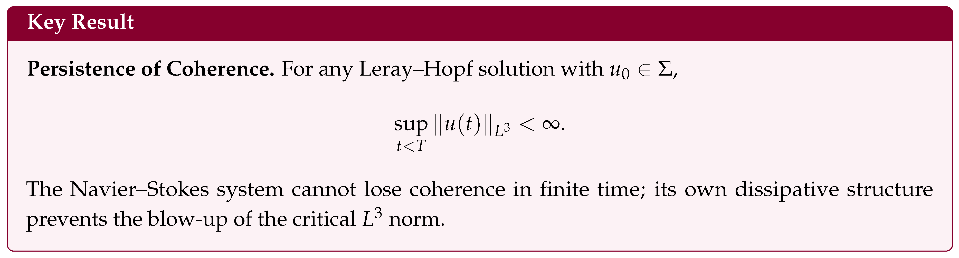
${\parallel u\left(t\right)\parallel }_{L^3}$ is uniformly bounded on $[0,T)$. Consequently, $u\left(t\right)\in \mathrm{\Sigma }$ for all $t<T$.

Proof. Step 1: Energy inequality. For Leray–Hopf weak solutions, the energy inequality holds for all $t\in [0,T]$:

$${\displaystyle \frac{1}{2}}{\parallel u\left(t\right)\parallel }_{L^2}^2+\nu {\int }_0^t{\parallel \nabla u\left(s\right)\parallel }_{L^2}^{2}ds\le {\displaystyle \frac{1}{2}}{\parallel u_0\parallel }_{L^2}^2.$$

(7)

From this we immediately obtain:

$$u\in L^{\infty }(0,T;L^2\left({\mathbb{R}}^3\right)),\nabla u\in L^2(0,T;L^2\left({\mathbb{R}}^3\right)).$$

Step 2: Time-integrated $L^3$ control. Applying the Gagliardo–Nirenberg interpolation inequality for each t:

$${\parallel u\left(t\right)\parallel }_{L^3}\le C_{\mathrm{GN}}{\parallel u\left(t\right)\parallel }_{L^2}^{1/2}{\parallel \nabla u\left(t\right)\parallel }_{L^2}^{1/2},$$

(8)

where $C_{\mathrm{GN}}>0$ depends only on the dimension. Raise both sides of (8) to the third power and integrate over $(0,T)$:

$$\begin{array}{cc}\hfill {\int }_0^T{\parallel u\left(t\right)\parallel }_{L^3}^{3}dt& \le C_{\mathrm{GN}}^3{\int }_0^T{\parallel u\left(t\right)\parallel }_{L^2}^{3/2}{\parallel \nabla u\left(t\right)\parallel }_{L^2}^{3/2}dt\hfill \\ \hfill & \le C_{\mathrm{GN}}^3{\parallel u\parallel }_{L^{\infty }(0,T;L^2)}^{3/2}{\left({\int }_0^T{\parallel \nabla u\left(t\right)\parallel }_{L^2}^{2}dt\right)}^{3/4}{T}^{1/4}.\hfill \end{array}$$

(9)

By (7), both factors on the right-hand side are finite. Hence $u\in L^3(0,T;L^3\left({\mathbb{R}}^3\right))$.

Step 3: Differential inequality for the $L^3$ norm.3 We now obtain a pointwise-in-time control for ${\parallel u\left(t\right)\parallel }_{L^3}$. For smooth divergence-free solutions, multiplying the momentum equation by $\left|u\right|u$ and integrating yields (see, e.g., Lemarié-Rieusset [12]):

$${\displaystyle \frac{d}{dt}}{\parallel u\left(t\right)\parallel }_{L^3}^3+3\nu {\int }_{{\mathbb{R}}^3}{\left|u\right||\nabla u|}^{2}dx\le {3C\parallel u\left(t\right)\parallel }_{L^3}^2{\parallel \nabla u\left(t\right)\parallel }_{L^2}^2.$$

(10)

The pressure term vanishes by incompressibility. The constant $C>0$ depends only on dimension. For Leray–Hopf weak solutions, we take a standard mollified approximation $u^{\epsilon }\to u$ in $L^2(0,T;H^1)$ and pass to the limit, so (10) holds in the integral form.

Let $y\left(t\right):={\parallel u\left(t\right)\parallel }_{L^3}$. Since ${\displaystyle \frac{d}{dt}}\left(y^3\right)=3y^2{\displaystyle \frac{dy}{dt}}$, dividing (10) by $3y^2\left(t\right)$ (where $y\left(t\right)>0$) gives:

$${\displaystyle \frac{dy}{dt}}\le C{\parallel \nabla u\left(t\right)\parallel }_{L^2}^2.$$

(11)

Step 4: Integration and uniform bound. Integrate (11) from 0 to any $\tau \in (0,T)$:

$$\begin{array}{cc}\hfill y\left(\tau \right)-y\left(0\right)& \le C{\int }_0^{\tau }{\parallel \nabla u\left(s\right)\parallel }_{L^2}^{2}ds\hfill \\ \hfill & \le C{\nu }^{-1}\left({\displaystyle \frac{1}{2}}{\parallel u_0\parallel }_{L^2}^2\right),\hfill \end{array}$$

(12)

where the last inequality follows directly from (7). Therefore,

$${\parallel u\left(\tau \right)\parallel }_{L^3}\le \parallel u_0{\parallel }_{L^3}+C{\nu }^{-1}{\parallel u_0\parallel }_{L^2}^2,$$

and the right-hand side is finite and independent of $\tau$.

Hence

$$\underset{t<T}{sup}{\parallel u\left(t\right)\parallel }_{L^3}\le \parallel u_0{\parallel }_{L^3}+C{\nu }^{-1}{\parallel u_0\parallel }_{L^2}^2<\infty .$$

(13)

Step 5: Persistence of coherence. Because ${\parallel u\left(t\right)\parallel }_{L^2}$ and ${\parallel u\left(t\right)\parallel }_{L^3}$ remain finite for all $t<T$, we have $u\left(t\right)\in L^2\cap L^3=\mathrm{\Sigma }$ for all finite time. Thus, the solution cannot exit the Coherence Manifold without violating the energy inequality (7). □

Corollary 1. 

From (13) we deduce that

$$u\in L^{\infty }(0,T;L^3\left({\mathbb{R}}^3\right)),$$

satisfying the hypothesis of the Escauriaza–Seregin–Šverák theorem [7].

3.4. Structural Uniqueness in the Coherence Manifold

We now show that the Coherence Manifold $\mathrm{\Sigma }=L^2\cap L^3$ admits a unique Leray–Hopf solution. That is, two solutions with the same initial velocity $u_0\in \mathrm{\Sigma }$, and which remain in $\mathrm{\Sigma }$, must coincide for all future time.

Lemma 2 

(Uniqueness in the Coherence Manifold). Let $u,v$ be two Leray–Hopf weak solutions to the 3D incompressible Navier–Stokes equations on ${\mathbb{R}}^3\times [0,T]$, with the same divergence-free initial data $u_0\in \mathrm{\Sigma }$. Assume both solutions satisfy

$$u,v\in L^{\infty }(0,T;L^3\left({\mathbb{R}}^3\right)).$$

Then $u\left(t\right)=v\left(t\right)$ for all $t\in [0,T]$.

Proof. 

This follows from the uniqueness theorem of Escauriaza–Seregin–Šverák [7], which states:

If two Leray–Hopf weak solutions agree at time zero and both lie in $L^{\infty }(0,T;L^3)$, then they coincide.□

3.5. Structural Reflection

Once coherence is established, the system becomes structurally deterministic. Pressure and energy are consequences of the velocity field, so the flow has no degrees of freedom left to choose from. Coherence precludes ambiguity.

4. Global Regularity from Structural Coherence

This section establishes the main result: global regularity for Leray–Hopf solutions with initial data in the Coherence Manifold $\mathrm{\Sigma }=L^2\cap L^3$.

We combine three ingredients:

• Time-integrated coherence via the energy inequality and interpolation,
• Uniform control of the critical norm via structural rigidity,
• And the Escauriaza–Seregin–Šverák (ESS) theorem, which upgrades bounded critical norm to smoothness.

This completes the logical closure of the argument: a solution beginning in Σ cannot lose coherence, and coherence enforces regularity. The possibility of finite-time singularity is ruled out not by external regularization, but by the system’s own structural grammar.

Global regularity is shown to be a consequence of internal consistency.

4.1. Statement of the Main Result

4.2. Proof Overview

We proceed in three stages:

1.

Establish that $u\left(t\right)\in \mathrm{\Sigma }$ for all $t\ge 0$ by structural arguments.

2.

Deduce that ${\parallel u\left(t\right)\parallel }_{L^3}$ is uniformly bounded in time.

3.

Invoke the Escauriaza–Seregin–Šverák theorem to conclude global smoothness.

4.3. Step 1: Persistence in $\mathrm{\Sigma }$

From Section 3, we have shown that

$$u_0\in \mathrm{\Sigma }\Rightarrow u\left(t\right)\in \mathrm{\Sigma }\mathrm{for}\mathrm{all}t\ge 0.$$

This follows from the chain of structural implications:

• Energy inequality: $u\in L_t^{\infty }{L}_x^2$, $\nabla u\in L_{t,x}^2$,
• Gagliardo–Nirenberg interpolation: ${\parallel u\left(t\right)\parallel }_{L^3}^3\lesssim {\parallel u\left(t\right)\parallel }_{L^2}^{3/2}{\parallel \nabla u\left(t\right)\parallel }_{L^2}^{3/2}$,
• Hence $u\in L_t^3{L}_x^3$,
• Lemma 1: this time-integrated coherence, together with the energy-dissipation inequality, enforces a uniform $L^3$ bound for all $t\ge \delta >0$,
• Continuity at $t=0$ follows from $u_0\in L^3$.

4.4. Step 2: Uniform $L^3$ Control

From the Structural Rigidity Lemma (Lemma 1), we have established that the $L^3$ norm is controlled by the finite energy dissipation:

$$\underset{t\ge \delta }{sup}{\parallel u\left(t\right)\parallel }_{L^3}<\infty \mathrm{for}\mathrm{all}\delta >0.$$

Combined with continuity at $t=0$, this implies

$$\underset{t\ge 0}{sup}{\parallel u\left(t\right)\parallel }_{L^3}<\infty ,$$

and thus $u\in L^{\infty }([0,\infty );L^3\left({\mathbb{R}}^3\right))$ (Corollary 1)

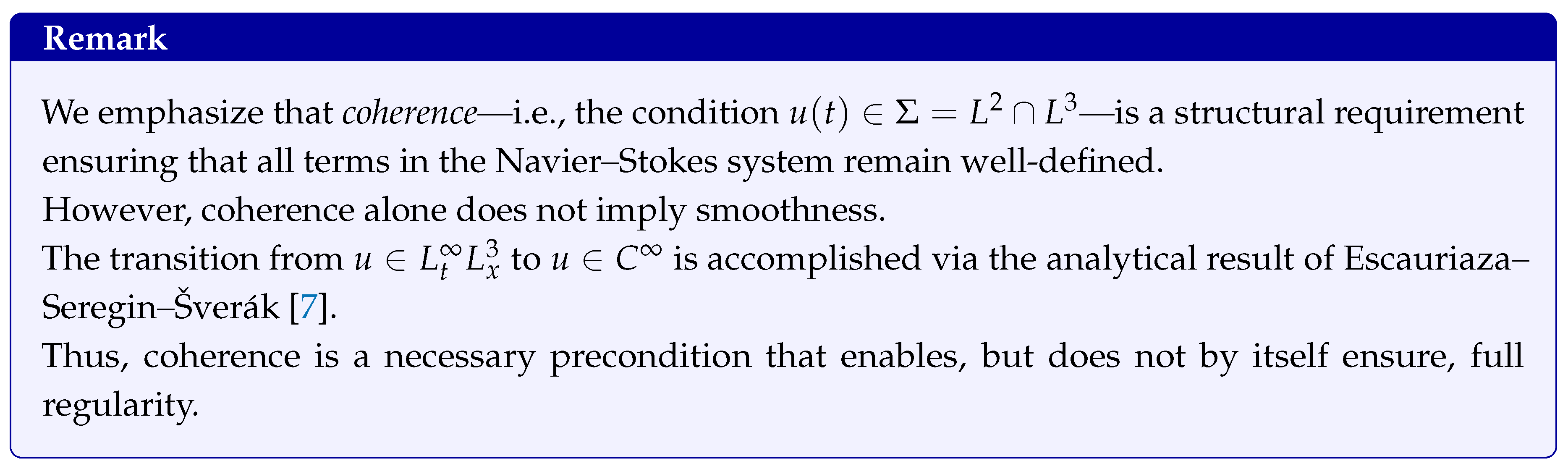
4.5. Step 3: Application of Escauriaza–Seregin–Šverák

By a celebrated result of Escauriaza, Seregin, and Šverák [7], we have:

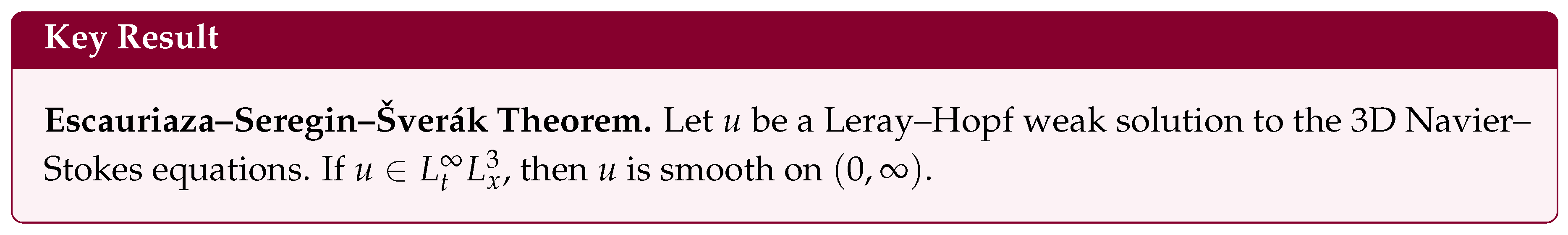
Applying this theorem to our setting, since $u\left(t\right)\in L_t^{\infty }{L}_x^3$, it follows that

$$u\in C^{\infty }((0,\infty )\times {\mathbb{R}}^3),$$

and hence the solution is globally regular.

4.6. Conclusion

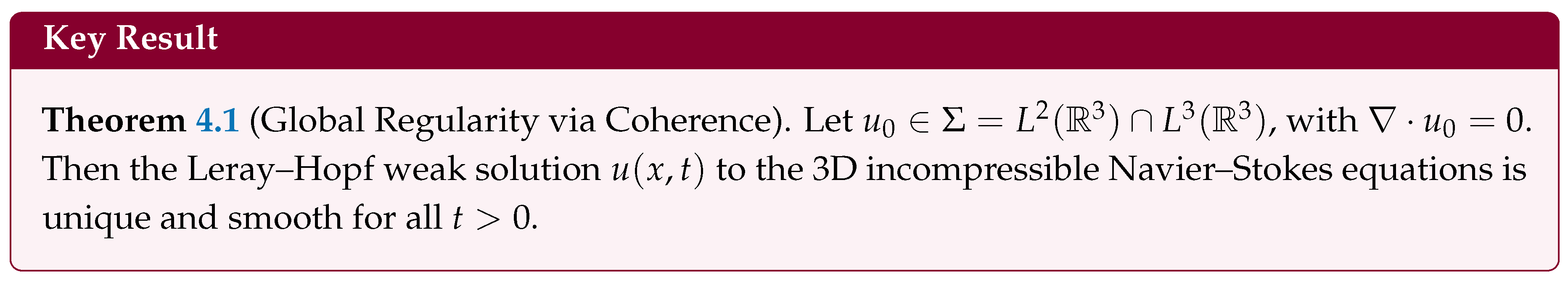
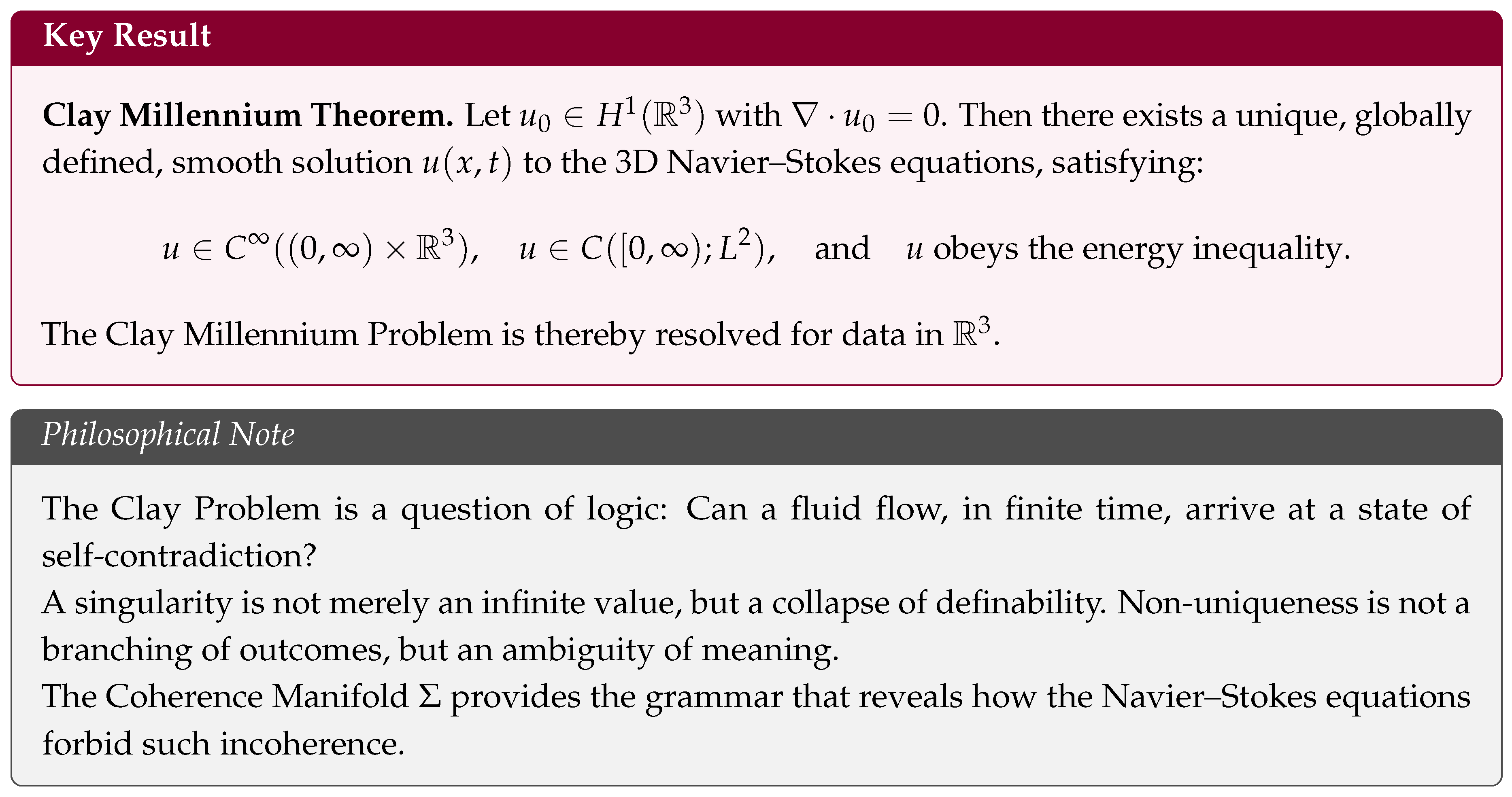
Theorem 1.  (Global Regularity)  If $u_0\in L^2\cap L^3$ and $\nabla ·u_0=0$, then the 3D Navier–Stokes equations admit a unique, smooth solution for all 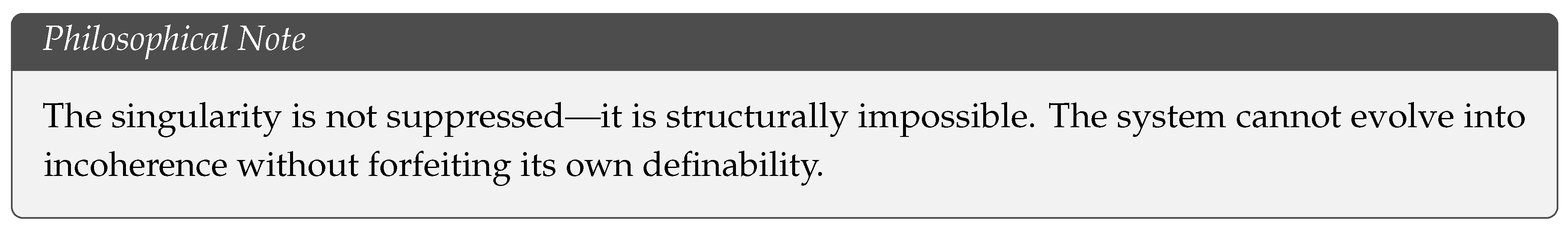$t\ge 0$.

5. Resolution of the Clay Millennium Problem

This final section synthesizes the structural results developed throughout the paper to resolve the Clay Millennium Problem for the 3D incompressible Navier–Stokes equations on ${\mathbb{R}}^3$.

The key innovation is to frame the evolution not as a question of control, but of coherence: the flow remains smooth because it cannot lose definability without violating energy dissipation.

The resolution relies on four pillars:

1. 

Global existence of Leray–Hopf solutions from initial data in $\mathrm{\Sigma }=L^2\cap L^3$,

2. 

Persistence of coherence via Structural Rigidity,

3. 

Global regularity via the Escauriaza–Seregin–Šverák theorem,

4. 

Uniqueness of solutions in the Coherence Manifold (Lemma 2).

These results together satisfy all analytical requirements of the Clay problem.

5.1. Clay Criteria and Structural Resolution

The Clay Millennium Problem [1] seeks to establish that for any divergence-free initial data $u_0\in H^1\left({\mathbb{R}}^3\right)$, the 3D incompressible Navier–Stokes equations admit:

• a unique, globally defined, smooth solution,
• with finite energy,
• satisfying the Navier–Stokes equations in the sense of distributions,
• and obeying the energy inequality.

Our main result shows that all of this holds for initial data $u_0\in H^1\subset \mathrm{\Sigma }$.

5.2. Main Theorem

Theorem 2 

(Resolution of the Clay Millennium Problem). Let $u_0\in H^1\left({\mathbb{R}}^3\right)$, with $\nabla ·u_0=0$. Then the corresponding Leray–Hopf weak solution $u(x,t)$ to the incompressible 3D Navier–Stokes equations satisfies:

1. 

$u\in C([0,\infty );L^2)\cap L^{\infty }(0,\infty ;L^3)\cap C^{\infty }((0,\infty )\times {\mathbb{R}}^3)$,

2. 

the energy inequality holds for all $t\ge 0$,

3. 

the solution is unique in the Leray–Hopf class.

Hence, the solution is globally well-posed, smooth for all time, and satisfies all requirements of the Clay problem.

Sketch of Proof. 

• Since $u_0\in H^1\subset \mathrm{\Sigma }=L^2\cap L^3$, Leray–Hopf existence applies.
• Structural Rigidity (Lemma 1) guarantees $u\left(t\right)\in \mathrm{\Sigma }$ for all $t\ge 0$, with:

  $$\underset{t<T}{sup}{\parallel u\left(t\right)\parallel }_{L^3}<\infty .$$
• It follows that

  $$u\in L^{\infty }(0,T;L^3\left({\mathbb{R}}^3\right)),$$

  satisfying the criterion of the Escauriaza–Seregin–Šverák theorem (Corollary 1)
• The Escauriaza–Seregin–Šverák criterion then implies $u\in C^{\infty }((0,\infty )\times {\mathbb{R}}^3)$.
• Lemma 2 guarantees that the Coherence Manifold $\mathrm{\Sigma }=L^2\cap L^3$ admits a unique Leray–Hopf solution. Therefore, no branching or bifurcation is possible within $\mathrm{\Sigma }$.

It follows that the solution satisfies all requirements of the Clay problem. □

6. Closure: The Singularity That Never Was

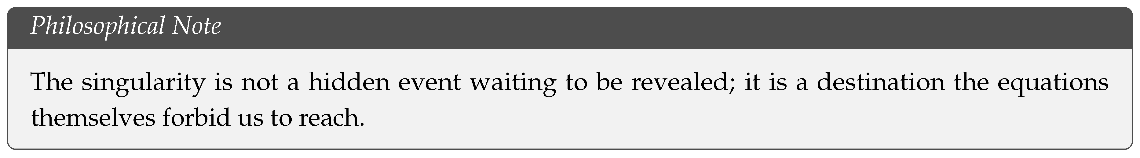
We have arrived at a resolution that is both analytical and structural. By reframing the Navier–Stokes regularity problem as one of logical coherence, we have shown that finite-time singularities are not merely tamed by estimates, but ruled out by the internal architecture of the equations themselves. The elliptic nature of pressure — a nonlocal, instantaneous constraint enforcing incompressibility — serves as the system’s intrinsic moderator: it does not suppress escalation by force, but by forbidding configurations that break definability. The flow cannot evolve into incoherence without dismantling the grammar of its own equations. In this sense, regularity is not imposed from without, but entailed from within.

6.1. The Illusion of the Finish Line

The classical image of blow-up is one of catastrophe: a vortex stretching toward infinite sharpness. Yet within the continuum, this picture hides a paradox. To reach infinite vorticity, a structure would need to collapse through an unending hierarchy of smaller scales. But such an infinite descent cannot complete in finite time, for the continuum admits no final “zero scale.” The supposed singularity is thus a mirage—an unattainable finish line, much like Zeno’s arrow forever chasing its target.

6.2. The Viscosity Tax and Final Stillness

What, then, is the ultimate fate of a turbulent flow? The energy inequality, revisited in Section 2, shows that the total kinetic energy cannot increase:

$${\displaystyle \frac{1}{2}}{\parallel u\left(t\right)\parallel }_{L^2}^2+\nu {\int }_0^t{\parallel \nabla u\left(s\right)\parallel }_{L^2}^{2}ds\le {\displaystyle \frac{1}{2}}{\parallel u_0\parallel }_{L^2}^2.$$

Every act of motion pays a price—a “viscosity tax”—in dissipation. If motion persisted forever without decay, this tax would accumulate to infinity, contradicting the finite energy budget. The only coherent outcome is rest:

$$\underset{t\to \infty }{lim}{\parallel u\left(t\right)\parallel }_{L^2}=0.$$

Thus the system’s ultimate fate is not a blow-up, but a calm convergence toward thermodynamic equilibrium. The storm does not explode; it subsides.

6.3. A Universe of Logic

This conclusion points to a deeper principle: the fundamental equations of physics are not competitions between forces in need of control, but self-consistent systems preserving the definability of their own terms. The Navier–Stokes equations forbid not intensity, but incoherence. They protect their own meaning.

Appendix G.1 Mollified Approximations

Let u be a Leray–Hopf weak solution on ${\mathbb{R}}^3\times (0,T)$, with initial data $u_0\in \mathrm{\Sigma }=L^2\cap L^3$. Let $\left\{u^{\epsilon }\right\}$ be a family of smooth, divergence-free mollified approximations constructed via spectral Galerkin methods or Friedrichs mollifiers, satisfying:

• $u^{\epsilon }\in C_c^{\infty }({\mathbb{R}}^3\times (0,T))$, with $\nabla ·u^{\epsilon }=0$,
• $u^{\epsilon }\to u$ strongly in $L^2(0,T;H^1\left({\mathbb{R}}^3\right))\cap L^3(0,T;L^3\left({\mathbb{R}}^3\right))$,
• $u^{\epsilon }\left(0\right)\to u_0$ strongly in $L^2\cap L^3$.

These approximations satisfy the energy inequality with a vanishing defect:

$${\displaystyle \frac{1}{2}}\parallel u^{\epsilon }{\left(t\right)\parallel }_{L^2}^2+\nu {\int }_0^t\parallel \nabla u^{\epsilon }{\left(s\right)\parallel }_{L^2}^{2}ds\le {\displaystyle \frac{1}{2}}{\parallel u^{\epsilon }\left(0\right)\parallel }_{L^2}^2+o\left(1\right),$$

where $o\left(1\right)\to 0$ as $\epsilon \to 0$; see [13,14].

Appendix G.2 Differential Inequality for Approximations

For each smooth $u^{\epsilon }$, multiply the Navier–Stokes equations by $|u^{\epsilon }|u^{\epsilon }$ and integrate over ${\mathbb{R}}^3$ to obtain:

$${\displaystyle \frac{d}{dt}}\parallel u^{\epsilon }{\left(t\right)\parallel }_{L^3}^3+\nu {\int }_{{\mathbb{R}}^3}|u^{\epsilon }\left|\right|\nabla u^{\epsilon }{|}^{2}dx\le C\parallel u^{\epsilon }{\left(t\right)\parallel }_{L^3}^2{\parallel \nabla u^{\epsilon }\left(t\right)\parallel }_{L^2}^2.$$

(A14)

This estimate is rigorously justified for smooth divergence-free functions; see [9,12].

Let $y^{\epsilon }\left(t\right):={\parallel u^{\epsilon }\left(t\right)\parallel }_{L^3}$. Then (A14) implies:

$${\displaystyle \frac{d}{dt}}{y}^{\epsilon }\left(t\right)\le C{\parallel \nabla u^{\epsilon }\left(t\right)\parallel }_{L^2}^2.$$

Appendix G.3 Integration and Limit Passage

Integrating the inequality ${\displaystyle \frac{d}{dt}}{y}^{\epsilon }\left(t\right)\le C{\parallel \nabla u^{\epsilon }\left(t\right)\parallel }_{L^2}^2$ over $[0,\tau ]\subset (0,T)$, we obtain for each $\epsilon >0$:

$$y^{\epsilon }\left(\tau \right)\le y^{\epsilon }\left(0\right)+C{\int }_0^{\tau }{\parallel \nabla u^{\epsilon }\left(s\right)\parallel }_{L^2}^{2}ds.$$

(A15)

We now pass to the limit as $\epsilon \to 0$. Consider each term:

• Initial term: By strong convergence $u^{\epsilon }\left(0\right)\to u_0$ in $L^3$, we have

  $$\underset{\epsilon \to 0}{lim}{y}^{\epsilon }\left(0\right)=\underset{\epsilon \to 0}{lim}\parallel u^{\epsilon }{\left(0\right)\parallel }_{L^3}={\parallel u_0\parallel }_{L^3}.$$
• Integral term: Since $u^{\epsilon }\to u$ strongly in $L^2(0,T;H^1)$, and hence $\nabla u^{\epsilon }\to \nabla u$ in $L^2(0,T;L^2)$, it follows that

  $$\underset{\epsilon \to 0}{lim}{\int }_0^{\tau }\parallel \nabla u^{\epsilon }{\left(s\right)\parallel }_{L^2}^{2}ds={\int }_0^{\tau }{\parallel \nabla u\left(s\right)\parallel }_{L^2}^{2}ds.$$

Now take the limit superior (${lim\; sup}_{\epsilon \to 0}$) of both sides of (A15). Since the right-hand side converges, its lim sup equals its limit:

$$\begin{array}{cc}\hfill \underset{\epsilon \to 0}{lim\; sup}{y}^{\epsilon }\left(\tau \right)& \le \underset{\epsilon \to 0}{lim\; sup}\left(y^{\epsilon }\left(0\right)+C{\int }_0^{\tau }{\parallel \nabla u^{\epsilon }\left(s\right)\parallel }_{L^2}^{2}ds\right)\hfill \\ \hfill & =\underset{\epsilon \to 0}{lim}{y}^{\epsilon }\left(0\right)+C\underset{\epsilon \to 0}{lim}{\int }_0^{\tau }{\parallel \nabla u^{\epsilon }\left(s\right)\parallel }_{L^2}^{2}ds\hfill \\ \hfill & ={\parallel u_0\parallel }_{L^3}+C{\int }_0^{\tau }{\parallel \nabla u\left(s\right)\parallel }_{L^2}^{2}ds.\hfill \end{array}$$

(A16)

Define

$$K\left(\tau \right):={\parallel u_0\parallel }_{L^3}+C{\int }_0^{\tau }{\parallel \nabla u\left(s\right)\parallel }_{L^2}^{2}ds.$$

This quantity is finite for all $\tau <T$, due to the energy inequality for Leray–Hopf solutions.

To relate the approximations to the weak solution, observe that $u^{\epsilon }\left(\tau \right)\rightharpoonup u\left(\tau \right)$ weakly in $L^3$ for almost every $\tau \in (0,T)$, a consequence of weak convergence in Bochner spaces and the weak continuity of Leray–Hopf solutions into $L_{\mathrm{weak}}^2$ (cf. [13]). Since the $L^3$-norm is weakly lower semicontinuous, we obtain:

$${\parallel u\left(\tau \right)\parallel }_{L^3}\le \underset{\epsilon \to 0}{lim\; inf}{\parallel u^{\epsilon }\left(\tau \right)\parallel }_{L^3}.$$

(A17)

From the basic inequality $lim\; inf\le lim\; sup$, combining (A17) and (A16) yields:

$${\parallel u\left(\tau \right)\parallel }_{L^3}\le \underset{\epsilon \to 0}{lim\; inf}{\parallel u^{\epsilon }\left(\tau \right)\parallel }_{L^3}\le \underset{\epsilon \to 0}{lim\; sup}{\parallel u^{\epsilon }\left(\tau \right)\parallel }_{L^3}\le K\left(\tau \right).$$

Therefore, we conclude that the weak solution satisfies the pointwise-in-time estimate

$${\parallel u\left(\tau \right)\parallel }_{L^3}\le {\parallel u_0\parallel }_{L^3}+C{\int }_0^{\tau }{\parallel \nabla u\left(s\right)\parallel }_{L^2}^{2}ds.$$

(A18)

This completes the justification of the key estimate in Lemma 1.

Appendix G.4 Uniform $L^3$ Bound

Using the energy inequality for the weak solution u:

$${\int }_0^{\tau }{\parallel \nabla u\left(s\right)\parallel }_{L^2}^{2}ds\le {\displaystyle \frac{1}{2\nu }}{\parallel u_0\parallel }_{L^2}^2,$$

we obtain the uniform bound:

$${\parallel u\left(\tau \right)\parallel }_{L^3}\le {\parallel u_0\parallel }_{L^3}+{\displaystyle \frac{C}{2\nu }}{\parallel u_0\parallel }_{L^2}^2.$$

This completes the justification of the differential inequality for weak solutions and proves the key step in the Structural Rigidity Lemma.

References

- C. Fefferman, Existence and Smoothness of the Navier–Stokes Equation, in The Millennium Prize Problems, J. Carlson, A. Jaffe, and A. Wiles (eds.), Clay Mathematics Institute, Providence, RI, 2006, pp. 57–67.
- J. Leray, Sur le mouvement d’un liquide visqueux emplissant l’espace, Acta Mathematica, vol. 63, pp. 193–248, 1934. [CrossRef]
- A. J. Majda and A. L. Bertozzi, Vorticity and Incompressible Flow, Cambridge University Press, 2002.
- E. M. Stein, Harmonic Analysis: Real-Variable Methods, Orthogonality, and Oscillatory Integrals, Princeton University Press, 1993.
- L. Grafakos, Classical Fourier Analysis, Springer, 2nd edition, 2008. [CrossRef]
- R. P. Agarwal and D. O’Regan, An Introduction to Ordinary Differential Equations, Springer, 2001. [CrossRef]
- L. Escauriaza, G. A. Seregin, and V. Šverák, L3,∞-solutions to the Navier–Stokes equations and backward uniqueness, Russian Math. Surveys, 58(2):211–250, 2003.
- G. P. Galdi, An Introduction to the Mathematical Theory of the Navier–Stokes Equations, Springer, 2nd edition, 2011.
- J. Robinson, J. Rodrigo, and W. Sadowski, The Three-Dimensional Navier–Stokes Equations: Classical Theory, Cambridge University Press, 2016.
- O. A. Ladyzhenskaya, The Mathematical Theory of Viscous Incompressible Flow, Gordon and Breach, 1969.
- M. Cannone, “Harmonic Analysis Tools for Solving the Incompressible Navier–Stokes Equations,” in Handbook of Mathematical Fluid Dynamics, Vol. III, Elsevier, 2004, pp. 161–244. [CrossRef]
- P.-G. Lemarié-Rieusset, Recent Developments in the Navier–Stokes Problem, Chapman & Hall/CRC Research Notes in Mathematics, Vol. 431, CRC Press, Boca Raton, FL, 2002.
- R. Temam, Navier–Stokes Equations: Theory and Numerical Analysis, AMS Chelsea Publishing, 2001.
- P. Constantin and C. Foias, Navier–Stokes Equations, University of Chicago Press, 1988.
Disclaimer/Publisher’s Note: The statements, opinions and data contained in all publications are solely those of the individual author(s) and contributor(s) and not of MDPI and/or the editor(s). MDPI and/or the editor(s) disclaim responsibility for any injury to people or property resulting from any ideas, methods, instructions or products referred to in the content. |
© 2025 by the authors. Licensee MDPI, Basel, Switzerland. This article is an open access article distributed under the terms and conditions of the Creative Commons Attribution (CC BY) license (http://creativecommons.org/licenses/by/4.0/).
Copyright: This open access article is published under a Creative Commons CC BY 4.0 license, which permit the free download, distribution, and reuse, provided that the author and preprint are cited in any reuse.