
Submitted:
25 April 2023
Posted:
25 April 2023
You are already at the latest version
Abstract
In this work, we propose a transition wave equation from quantum to classical regime in the framework of the von Neumann formalism for ensembles and then obtain an equivalent scaled equation. This leads us to develop a scaled statistical theory following the well-known Wigner-Moyal approach of quantum mechanics. This scaled nonequilibrium statistical mechanics has in it all the ingredients of the classical and quantum theory described in terms of a continuous parameter displaying all the dynamical regimes in-between the two extreme cases. Finally, a simple application of our scaled formalism consisting of reflection from a mirror by computing various quantities including probability density plots, scaled trajectories and arrival times are analyzed.
Keywords:
Bohmian mechanics
; Transition wave equation
; Scaled Liouville-von Neumann equation
; Scaled trajectories
; Scaled Wigner-Moyal approach
; Scaled Wigner distribution function
1. Introduction
The most general formulation of quantum mechanics is given in terms of a density operator, a statistical mixture of state vectors. Furthermore, in an open or composite quantum system, the system of interest is described by the reduced density operator which is obtained by tracing out the total density operator over the remaining degrees of freedom. Using the method of protective measurements, Anandan and Aharonov have proposed the observation of the density matrix of a single system, thus presenting a new meaning of the density matrix in this context [1]. In this regard, it has been shown that the density matrix can be consistently treated as a property of an individual system, not of an ensemble alone [2]. In addition to the statistical (mixture) and reduced density matrices, the conditional density matrix, conditional on the configuration of the environment, has been discussed [3] and argued that the precise definition is possible only in Bohmian mechanics.
On the other hand, Bohmian mechanics [4,5,6,7] is clearly a complementary, alternative and new interpretive way of introducing quantum mechanics, providing a clear picture of quantum phenomena in terms of trajectories in configuration space. A gradual decoherence process could then be devised by using the so-called quantum-classical transition differential wave equation, originally proposed by Richardson et al. [8] for conservative systems. Doing so, the corresponding dynamics are governed by a continuous parameter, the transition parameter, leading to a continuous description of any quantum phenomena in terms of trajectories, scaled trajectories [9,10]. In other words, one is thus able to describe any dynamical regime in-between the quantum and classical ones in a continuous way emphasizing how this decoherence process is established (a scaled Planck’s constant is defined in terms of the transition parameter covering the limit ). Scaled trajectories also display the well-known non-crossing property even in the classical regime. Chou applied this wave equation to analyze wave-packet interference [11] and the dynamics of the harmonic and Morse oscillators with complex trajectories [12]. Stochastic Bohmian and scaled trajectories have also been discussed in the literature for open quantum systems [13]. Moreover, by assuming a time-dependent Gaussian ansatz for the probability density, Bohmian and scaled trajectories are expressed as a sum of a classical trajectory (a particle property) and a term containing the width of the corresponding wave packet (a wave property) within of what has been called the dressing scheme [7]. Analogously, this scheme is also observed in the context of nonlinear quantum mechanics [14] where, for example, solitons also possess this wave-particle duality; their wave property appears in the form of a travelling solitary wave and their corpuscle feature is analogous to a classical particle.
The procedure of using a continuous parameter monitoring the different dynamical regimes in the theory reminds us to the well-known WKB approximation, widely used also for conservative systems. Several key differences are worth stressing here. First, the classical Hamilton-Jacobi equation for the classical action is obtained at zero order in this approximation whereas the so-called classical wave (nonlinear) equation [15] is reached by construction. Second, the hierarchy of the differential equations for the action at different orders of the expansion in ℏ is substituted by only a transition differential wave equation which can be solved in the linear and nonlinear domains. Third, the transition from quantum to classical trajectories is carried out in a continuous and gradual way, stressing the different dynamical regimes in-between the quantum and classical ones. And fourth, this continuous transition can also be seen as a gradual decoherence process (let us say, internal decoherence) due to the scaled Planck’s constant, allowing us to analyze what happens at intermediate regimes [16]. However, decoherence effects have also been analyzed in interference phenomena using a class of quantum trajectories, based on the same grounds as Bohmian ones, associated with the system reduced density matrix [17]. Such a study has been carried out for statistical mixtures and studied in the framework of Bohmian mechanics [18], the minimal view i.e., without any reference to the quantum potential. Even more, by writing the density matrix in polar form, a Bohmian trajectory formulation for dissipative systems has been proposed where a double quantum potential being a measure of the local curvature of the density amplitude is responsible for quantum effects [19]. A different approach has been taken for the hydrodynamical formulation of mixed states [20] where a local-in-space formulation has been adopted in the sense that a hierarchy of moments contains the non-local information associated with the off-diagonal elements of the density matrix.
In the present article, our purpose is to provide a clear formulation of pure and mixed ensembles in terms of the Bohmian mechanics by using the polar form of the density matrix within the von Neumann equation framework. In this way, the corresponding quantum potential is introduced, and a momentum vector field is defined for both forward and backward in time motions. Once this is carried out, within the quantum-classical transition equation framework, a scaled Schrödinger equation is easily derived leading to the so-called scaled von Neumann equation. Afterwards, Moyal’s procedure [21] used to interpret quantum mechanics as a statistical theory is then applied to the scaled theory by considering a characteristic function which is a standard function in statistical mechanics [22]. The expectation value of the so-called Heisenberg-Weyl operator [23] is treated as the characteristic function. Then, the inverse Fourier transform of the characteristic function is considered as the probability distribution function and its time evolution was thus obtained. In this way, the classical Liouville equation is again derived within this scaled theory. The foundations of nonequilibrium statistical mechanics are based on the Liouville equation which is assocaited with a Hamiltonian dynamics (in general, in phase space). In other words, with this theoretical analysis, we have clearly shown that a scaled statistical mechanics is well established and ready to be applied. This new nonequilibrium statistical mechanics would be valid for any dynamical regime, going from the quantum to the classical ones. As a simple illustration of our new formulation, scattering of a statistical mixture of Gaussian wave packets from a hard wall is studied and compared to the corresponding superposed state. The application of the new scaled nonequilibrium statistical mechanics will be postponed for a future work.
2. Theory
When an isolated physical system is described by a density operator instead of a state vector , the equation of motion ruled by the density operator is the so-called Liouville-von Neumann equation or simply von Neumann equation which is written as
where is the Hamiltonian operator of the system and represents the commutator of two operators. For a single particle and in one dimension, this Hamiltonian is expressed as
where the first term is the kinetic energy operator and the second one, the external interaction potential, . This equation reads as
in the position representation. Diagonal elements of the density matrix give probabilities while the non-diagonal elements represent coherences.
2.1. Pure Ensembles in the de Broglie-Bohm Approach
Before considering mixed ensembles, it is important first to look at pure ones in the framework of the von Neumann equation. Density operator elements, in coordinate representation, for the pure state are given by where the wave function is governed by the Schrödinger equation
and its complex conjugate is governed by the complex conjugation of the same equation i.e.,
This equation reveals that is the wave function corresponding to the time-reversed state [24]. Writing the wave function in its polar form
and being both real functions the amplitude and phase of the wave function, respectively. By substituting this polar form in Eq. (4) and splitting the resultant equation in its real and imaginary parts, one obtains
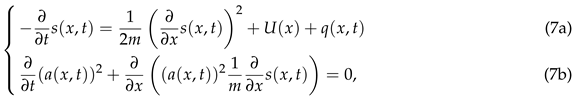 which are respectively the generalized Hamilton-Jacobi and the continuity equations where
is the well-known quantum potential. These equations suggest the definition of the momentum field as
and the velocity field as
which are respectively the generalized Hamilton-Jacobi and the continuity equations where
is the well-known quantum potential. These equations suggest the definition of the momentum field as
and the velocity field as
which are respectively the generalized Hamilton-Jacobi and the continuity equations where
Bohmian trajectories are thus constructed from the guidance equation as
being the initial position.
By applying the operator to Eq. (7a) and using Eq. (10), one reaches a Newtonian like equation according to
which shows that regarding as a potential on the same footing as is consistent.
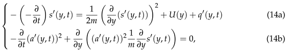
Now let us consider evolution of . As stated above, its evolution is governed by Eq. (5) and expressed again in polar form
one has that
 where
where
where
By comparison to Eqs. (7a) and (7b), has been replaced by as the result of time reversal. With respect to these new equations, one defines the momentum field, in the y direction, as
which using Eqs. (14a) and (14b) yields again a Newtonian like equation
Note that the minus sign in Eq. (16) reflects the time-reversed dynamics in the y direction [19]. However, note that a comparison between Eq. (6) and Eq. (13) reveals that
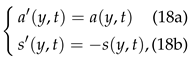 and, as one expects, .
and, as one expects, .By subtracting now Eq. (14a) from Eq. (7a), and using Eqs. (18a) and (18b) we have that
Multiplying Eq. (7b) by and Eq. (14b) by , subtracting the resulting equations and using Eqs. (18a) and (18b) yields
Note that the real functions and appearing in Eqs. (19) and (20) are the amplitude and phase of the pure density matrix, respectively
One could directly reach Eqs. (19) and (20) by introducing this polar form in the von Neumann equation (3).
2.2. Mixed Ensembles in the de Broglie-Bohm Framework
Let us now consider a mixed state. The hermiticity of the density operator implies
From this property and the polar form of the density matrix
one has that
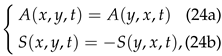 i.e., the amplitude (phase) of the density matrix is symmetric (antisymmetric) under the interchange. Now, by introducing Eq. (23) into the von Neumann equation (3) and splitting the resultant equation in real and imaginary parts, one again obtains the Hamilton-Jacobi equation for the phase
and the continuity equation
for the amplitude where
is again the corresponding quantum potential. By defining the two-component momentum vector field as
Eq. (26) can be written in compact form as
or
where we have introduced the velocity vector field
Eq. (29) can thus be written as the usual continuity equation
for the conservation of in the two-dimensional space represented by x and y,
i.e., the amplitude (phase) of the density matrix is symmetric (antisymmetric) under the interchange. Now, by introducing Eq. (23) into the von Neumann equation (3) and splitting the resultant equation in real and imaginary parts, one again obtains the Hamilton-Jacobi equation for the phase
Using Eqs. (28) and (25), one obtains the quantum Newton-like equation as
where the + (−) sign inside the parentheses stands for x (y) component of the momentum field.
If one uses the center of mass and relative coordinates according to
 Eq. (29) is rewritten as
Eq. (29) is rewritten as
Note that this equation can also be directly obtained from the von Neumann equation in the coordinates,
From Eq. (24a), it is seen that is an even function of the relative coordinate r and thus its derivative with respect to r is odd under . This implies that the last term of Eq. (36) is zero for , i.e., when considering diagonal elements. From this analysis, one arrives to
for the conservation of probability, i.e., diagonal elements of the density matrix, , from which the Bohmian velocity field is obtained as follows
Note that this velocity field can also be deduced from the probability current density
through the ratio .
2.3. The Scaled von Neumann Equation: A Proposal for Quantum-Classical Transition
In an effort to describe a quantum-to-classical continuous transition, the following non-linear transition equation was proposed to be in the Schrödinger framework
containing the so-called transition parameter ϵ going from one (quantum regime) to zero (classical regime) and in-between. The equivalent scaled linear equation reads now as
which was shown elsewhere [8], the so-called scaled Planck constant being
This study has been generalized to dissipative systems in the framework of the Caldirola-Kanai [10] and the Kostin or the Schrödinger-Langevin [9] equations. Here our purpose is to generalize this previous study to the von Neumann formalism of ensembles.
The last term of Eq. (25), the quantum potential, is responsible for quantum effects. Following Rosen [25], by subtracting this term to the von Neumann equation and after splitting again the real and imaginary parts, we reach the classical Hamilton-Jacobi equation, Eq. (25), without the quantum potential. Because of this, we could call this equation the classical von Neumann equation (a similar classical Liouville equation could also be reached) which reads as follows
where the sub-index “cl” refers to “classical” and means the modulus of . Now, following [8], the transition equation is proposed to be
From the polar form for the density matrix
one obtains
Now, multiplying Eq.(47a) by
and Eq. (47b) by , and adding the resulting equations, after some straightforward algebra one obtains
This is the so-called scaled von Neumann equation. The form of this scaled equation is exactly the
same as that of the von Neumann equation. The only changes are that ℏ and ρ have been replaced by the corresponding scaled quantities ℏ and ρ. Thus, the structure of the continuity equation is the same
and one has
for the scaled probability density current from which the scaled velocity is derived
Finally, the scaled trajectories are determined by integrating the guidance equation
being the initial position of the particle.
We now consider Ehrenfest relations. We first write the scaled von Neumann equation (49) in the form
where the scaled Hamiltonian operator in the position representation is
Now for the time derivative of the arbitrary time-independent observable one has that
where we have used Eq. (53) and the cyclic property of the trace operation. Note, however, that one
should take care of using this property when the dimension of the vector space is infinite. Then, from
Eq. (55), one obtains the usual Ehrenfest relations
2.4. The Scaled Wigner-Moyal Approach
Moyal [21] attempted to interpret quantum mechanics as a statistical theory. He started with the
characteristic function, a standard tool of statistical theory but in the unusual way [22]; the expectation
value of the so-called Heisenberg-Weyl operator [23] was treated as the characteristic function. Then,
the inverse Fourier transform of the characteristic function was considered to be the probability
distribution function and its time evolution was thus obtained from the standard methods of statistical
mechanics. Interestingly enough, the same evolution equation can be reached by starting from the
density operator satisfying the standard quantum mechanical Liouville-von Neumann equation. In
spite of seemingly different starting points, Hiley [22] has shown they are, in fact, the same starting
point. We are going to follow the same procedure but in the scaled theory context.
Using the Fourier transform of the scaled wavefunction, the corresponding pure scaled density
matrix can be written
and using again the R and r coordinates for space and similarly and for momentum, the density matrix can be transformed into
This equation shows that the function is the partial Fourier transform of the scaled
density matrix with respect to the relative coordinate r. Thus, one has that
which is just the scaled Wigner distribution function (see Ref. [26] for comparison). This can be explicitly
seen by changing the relative variable r → −r/2. The time evolution of the scaled Wigner distribution function can be found from Eqs. (59) and (49), written in the coordinates r and R, according to
where we have defined the kernel
Thus, one has finally that
In the so-called Wigner-Moyal approach to quantum mechanics and said before, Moyal’s starting
point [21] is the Heisenberg-Weyl operator defined as
and its expectation value considered as the characteristic function,
Now, the same procedure could be followed in this context and write
which the phase space probability distribution function is the Fourier transform of the characteristic function
In the second line of Eq. (65), we have used the fact that the momentum operator is the generator
of translations. As Moyal proposed, one could also consider as a distribution function and
apply the corresponding standard methods of mechanical statistics. Starting from the Heisenberg
equation of motion
for the scaled operator , and following Moyal original work [21], one arrives at
where H(x, p) is the classical Hamiltonian; and and operates only on and so forth.
In the classical limit 0, this equation reduces to the well-known Liouville equation for the phase
space distribution function,
where stands for the Poisson bracket.
Thus, we have built a scaled nonequilibrium statistical mechanics from its fundamentals which
takes into account in a continuous way all the dynamical regimes in-between the two extreme case, the
quantum and classical ones.
3. Results and Discussion
As a simple application of our theoretical formalism, let us consider scattering from a hard wall at the origin
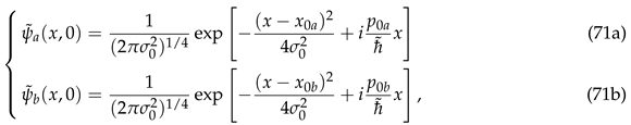
and two scaled Gaussian wave packets and with the same width but different centers and (initially localized in the left side of the wall) and kick momenta and i.e.,
 and build the superposition state at any time as
and the corresponding mixture
where is the step function and the normalization constant. Note that the unitary evolution of the scaled wave functions under the corresponding von Neumann equation keeps purity of states which is quantified from . By using now the propagator for the hard wall potential [27]
one obtains that
where the sub-index “f" stands for “free" and the corresponding propagator is written as
Now, from Eq. (75), one reaches
where
and build the superposition state at any time as
and the corresponding mixture
where is the step function and the normalization constant. Note that the unitary evolution of the scaled wave functions under the corresponding von Neumann equation keeps purity of states which is quantified from . By using now the propagator for the hard wall potential [27]
one obtains that
where the sub-index “f" stands for “free" and the corresponding propagator is written as
Now, from Eq. (75), one reaches
where
 being the complex width and the center of the freely propagating Gaussian wavepacket, respectively. The same holds for the b component of the wave function replacing only a by “b".
and build the superposition state at any time as
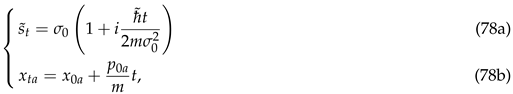
being the complex width and the center of the freely propagating Gaussian wavepacket, respectively. The same holds for the b component of the wave function replacing only a by “b".In Figure 1 and Figure 2 scaled probability density plots for the superposition of two Gaussian wave packets, Eq. (72), and for the mixed state, Eq. (73), for different dynamical regimes: (left top panel), (right top panel), (left bottom panel) and (right bottom panel). In both figures, the following initial parameters have been used for the calculations: , , , , and . As can clearly be seen in both cases, when the transition parameter is approaching zero (the classical dynamics regime), the interference pattern in collision between both states as well as in the scattering from the hard wall tends to be washed up in a continuous way. As one expects, when approaching the classical regime, results for the pure and the mixed states also become closer.
Let us discuss now how the scaled trajectories behave in the different dynamical regimes, going from Bohmian trajectories () to pure classical ones (). In Figure 3, a selection of scaled trajectories is plotted for the scaled wave function (left column) and the scaled density matrix (right column) for the quantum regime (top panels) and the nearly classical dynamical regime (bottom panels). The same units and initial parameters are used as previously. Comparison with the Figure 1 and Figure 2 reveals that trajectories follow the wave packets. In addition, although it is not apparent from our figure, but if one had selected the distribution of the initial positions according to the Born rule then he/she saw compact trajectories in regions with higher values of probability distribution. In other words, if trajectories obey the Born rule initially, they will do forever. The non-crossing rule of trajectories is still observed at nearly classical regime and even in the classical regime which is a consequence of the first order classical theory in contrast to the true second order theory. As the classical regime is approaching, the corresponding trajectories become more localized simulating two classical collisions, the first one coming from the scattering between the two wave packets and the second from the wall. However, only the wave packet starting closer to the hard wall is reflected by the wall due to the second collision. As has also been discussed elsewhere [28], wave packet interference can also be understood within the context of scattering off effective potential barriers. In classical mechanics, one can always substitute a particle-particle collision by that of an effective particle interacting with a potential. This fact is clearly observed in this context both for the superposition wave packet as well as for the density matrix.
From the non-crossing property of Bohmian trajectories, Leavens [29] proved that the arrival time distribution is given by the modulus of the probability current density. Following the same procedure for the scaled trajectories, one has that the scaled arrival time distribution at the detector place X can be expressed as
Moreover, the mean arrival time at the detector location and the variance in the measurement of the arrival time which is also a measure of the width of the distribution are respectively given by
As a result of the previous analysis in terms of scaled trajectories, these quantities are easily calculated.
In Figure 4, scaled arrival time distributions have been plotted at the detector location for the pure state (38) (left top panel) and the mixed state (39) (left bottom panel) for three different dynamical regimes: (green curve), (red curve) and (black curve). On the right top and bottom panels, the scaled mean arrival time and variance versus the transition parameter for the pure state (orange circled) and the mixed state (violet triangle up) have been also displayed. As clearly seen, the mean arrival time diminishes when going from the quantum to classical regime. This is related to the width of the probability distribution which is wider for the quantum regime than for the classical one. Furthermore, some differences between results coming from for the pure and mixed states seems to appear only around the quantum regime.
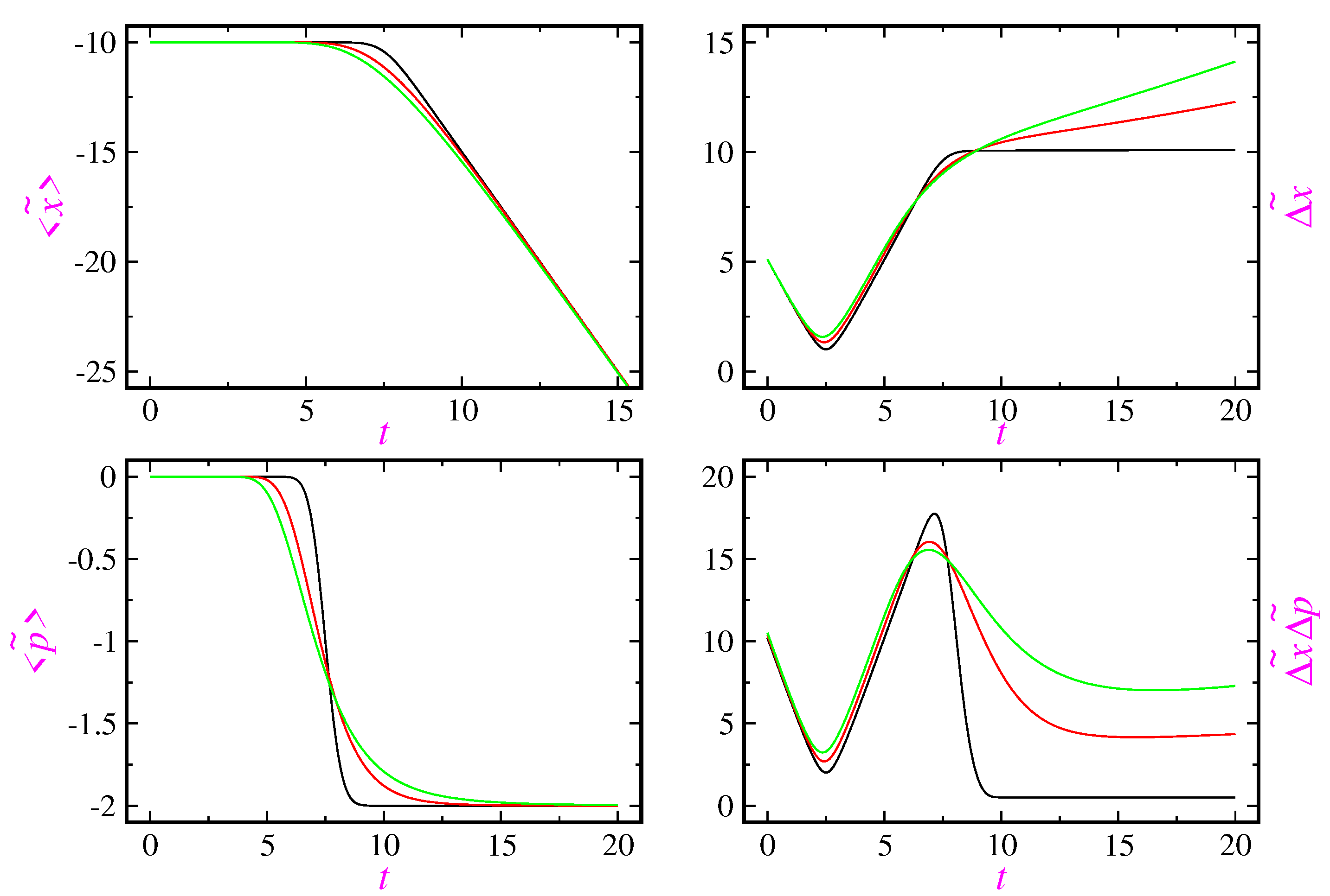
In Figure 5 the expectation value of position operator (left top panel), uncertainty in position (right top panel), expectation value of momentum operator (left bottom panel) and the product of uncertainties for the scaled mixed state for three different dynamical regimes: (green curves), (red curves) and (black curves) are plotted. The same initial parameters are used as in previous figures. This figure shows that the continuous transition from the quantum to classical dynamical regime present several global and important features: (i) reflection from the wall is delayed on average; (ii) the average velocity in reflection decreases; (iii) the uncertainty in position which is also a measure of width of the state diminishes and (iv) the product of uncertainties also decreases at long times. Furthermore, the Heisenberg uncertainty relation holds in any dynamical regime.
An interesting quantity is the non-classical effective force defined via
From the mixture (73) one has that
where is the expectation value of the momentum operator with respect to the component wavefunction . From the scaled Schrödinger equation (42) and boundary conditions on the wavefunction and its space derivative one obtains
Finally, from Eqs. (83) and (84) one has that
Classically there is no force in the region . In this regime, particles’ momentum reverses suddenly at the collision time with the hard wall, however this is not the non-classical case as the left-bottom panel of Figure 5 shows. Only classical particles with initial positive momentum, (in our case, particles described by ) collide with the wall which, for our initial parameters, collision time is .
4. Conclusions
Along the last years, we have shown that scaled trajectories provide an alternative and complementary view of the so-called quantum-to-classical transition within a theoretical scheme similar to the well-known WKB approximation. The (internal) decoherence process is also well and continuously established when approaching to the classical limit. The tunneling effect as well as the diffusion problem within the Langevin framework have been succesfully applied. In this work, we have extended this theoretical formalism in the same direction to propose a scaled Liouville-von Neumann equation and its Wigner representation which is precisely the first step to build a scaled nonequilibrium statistical mechanics. This was carried out following the same procedure proposed by Moyal long time ago in the context of standard quantum mechanics. This approach opens up new avenues to develop consisting of, for example, a scaled Fokker-Planck equation, analysis of phase transitions, space-time correlation functions, master equations, reaction rates and the so-called Kramers’ problem, kinetic models, linear response theory, projection operators, mode-coupling theory, nonlinear transport equations and much more. For example, the book by Zwanzig [30] could be a good guide to follow in the near future.
5. Dissipative Quantum Systems
In this section we consider an open quantum system taking into account only dissipation in the framework of the Caldirola-Kanai (CK) equation. In this context, evolution of the state vector is governed by
where is dissipation rate or friction coefficient. This equation can be straightforwardly generalized for mixed ensembles as
Introducing the polar form (20) of the density matrix in this equation and splitting the resultant equation in real and imaginary parts one obtains the Hamilton-Jacobi equation
with now the quantum potential
and the continuity equation (32) but with now the momentum vector field
and the corresponding Newtonian-like equation
where upper (lower) sign stands for x (y) component of the momentum field.
Again the dissipative transition equation
is proposed for smooth transition from quantum to classical mechanics. Using the similar analysis as
the previous section one gets the equivalent scaled equation
with the scaled probability current density
from which scaled trajectories can be constructed via the guidance equation
.
Author Contributions
Software: S.V.M.; conceptualization: S.V.M. and S.M-A.; methodology: S.V.M. and S.M-A.;
resources and supervision: S.V.M. and S.M-A.; writing-original draft preparation, S.V.M.; writing-review and
editing, S.V.M. and S.M-A. All authors have read and agreed to the published version of the manuscript.
Funding
This research was funded by the University of Qom and the Fundación Humanismo y Ciencia.
Data Availability Statement
Not applicable
Acknowledgments
SVM acknowledges support from the University of Qom and SMA from the Fundación Humanismo y Ciencia.
Conflicts of Interest
The authors declare no conflict of interest.
References
- J. Anandan and Y. Aharonov, Found. Phys. Lett. 12, 571 (1999).
- O. J. E. Maroney, Found. Phys. 35, 493 (2005).
- D. Dürr, S. Goldstein, R. Tumulka and N. Zanghi, Found. Phys. 35, 449 (2005).
- P. R. Holland, The Quantum Theory of Motion, Cambridge University Press, 1993.
- A. S. Sanz and S. Miret-Artés, A Trajectory Description of Quantum Processes. Part I. Fundamentals. Lecture Notes in Physics, Vol. 850, 2012.
- A. S. Sanz and S. Miret-Artés, A Trajectory Description of Quantum Processes. Part II. Applications. Lecture Notes in Physics, Vol. 831, 2014.
- A. B. Nassar and S. Miret-Artés, Bohmian Mechanics, Open Quantum Systems and Continuous Measurements, Springer, Heidelberg, 2017.
- C. D. Richardson, P. Schlagheck, J. Martin, N. Vandewalle and T. Bastin, Phys. Rev. A 89 (2014) 032118.
- S.V. Mousavi and S. Miret-Artés, Ann. Phys. 393 (2018) 76.
- S.V. Mousavi and S. Miret-Artés, J. Phys. Commun. 2 (2018) 035029.
- C.-C. Chou, Ann. Phys. 371 (2016) 437.
- C.-C. Chou, Int. J. Quan. Chem. 116 (2016) 1752.
- S.V. Mousavi and S. Miret-Artés, Found. Phys. 52 (2022) 78.
- P. Xiao-Feng and F. Yuan-Ping, Quantum Mechanics in Nonlinear Systems, World Scientific, Hong Kong, 2005.
- R. Schiller, Phys. Rev. 125 (1962) 1100.
- S.V. Mousavi and S. Miret-Artés, J. Phys. A: Math. Theor. 55 (2023) 475302.
- A. S. Sanz and F. Borondo, Eur. Phys. J. D 44, 319 (2007).
- A. Luis and A. S. Sanz, Ann. Phys. 357, 95 (2015).
- J. B. Maddoxa and E. R. Bittner, J. Chem. Phys. 115, 6309 (2001).
- I. Burghard and L. S. Cederbaum, J. Chem. Phys. 115, 10303 (2001).
- J. E. Moyal, Proc. Cam. Phil. Soc. 45, 99-123 (1949).
- B. J. Hiley, arXiv:1408.5680 [quant-ph].
- B. J. Hiley, J. Comput. Electron 14, 869-878 (2015).
- J. J. Sakurai and San Fu Tuan (editor), Modern Quantum Mechanics Revised Edition, Addison-Wesley Publishing Company, 1994.
- N. Rosen, Am. J. Phys. 32, 597 (1964).
- E. Wigner, Phys. Rev. 40, 749-59 (1932).
- C. Grosche and F. Steiner, Handbook of Feynman Path Integrals, Springer-Verlag Berlin Heidelberg, 1998.
- A. S. Sanz and S. Miret-Artés, J. Phys. A: Math. Theor. 41 (2008) 435303-1,23.
- C. R. Leavens, Bohm Trajectory Approach to Timing Electrons, In: J. Muga, R. S. Mayato and I. Egusquiza (eds) Time in Quantum Mechanics. Lecture Notes in Physics, vol 734. Springer, Berlin, Heidelberg 2008.
- R. Zwanzig, Nonequilibrium Statistical Mechanics, Oxford University Press, 2001.
Figure 1.
Scaled probability density plots for the superposition of two Gaussian wave packets, Eq. (38), for different regimes: (left top panel), (right top panel), (left bottom panel) and (right bottom panel). We have used as initial parameters, , , , , and .
Figure 1.
Scaled probability density plots for the superposition of two Gaussian wave packets, Eq. (38), for different regimes: (left top panel), (right top panel), (left bottom panel) and (right bottom panel). We have used as initial parameters, , , , , and .
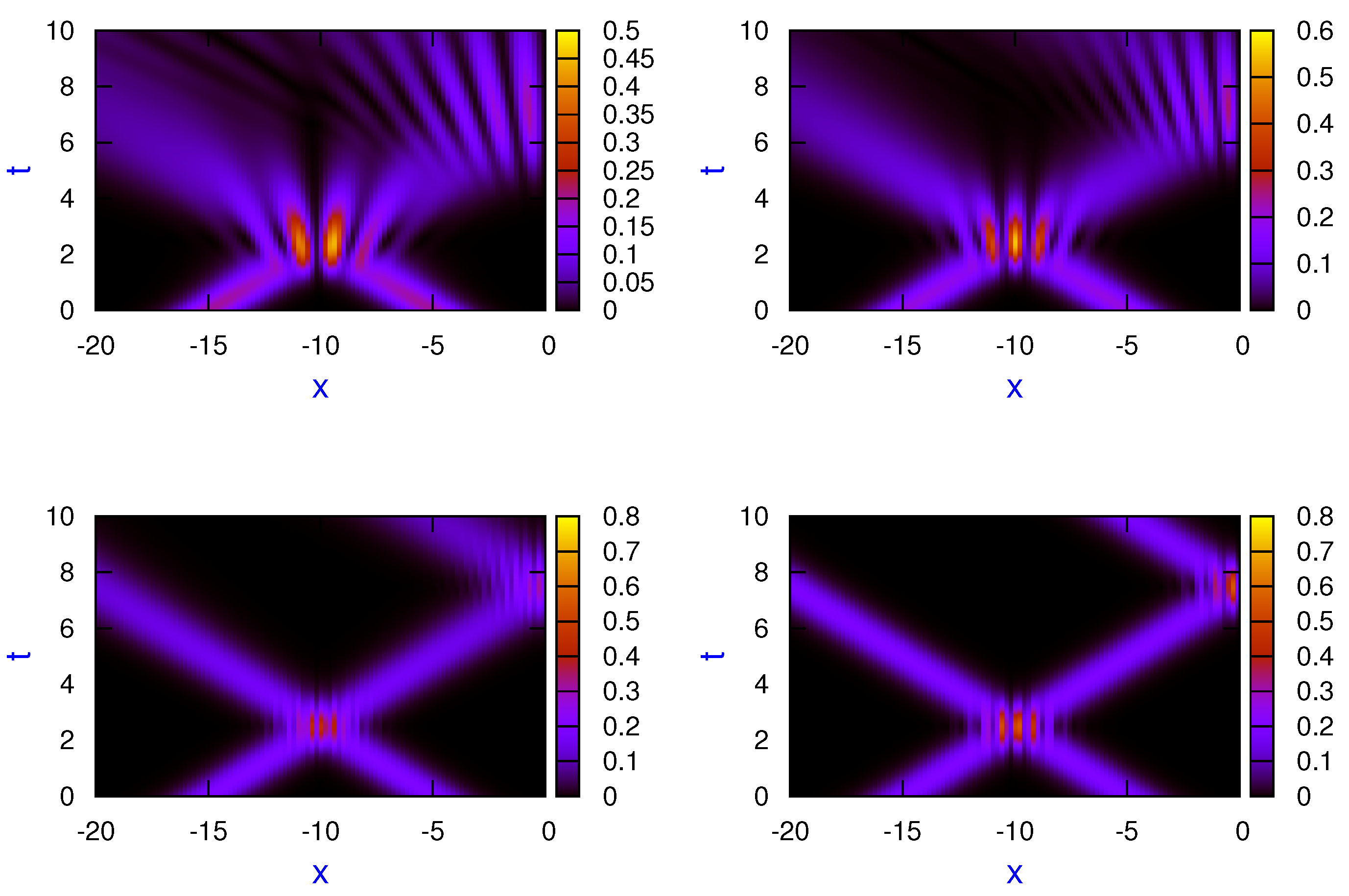
Figure 2.
Scaled probability density plots for the mixed state, Eq. (39), for different regimes: (left top panel), (right top panel), (left bottom panel) and (right bottom panel). The same initial parameters as Figure 1 have been used.
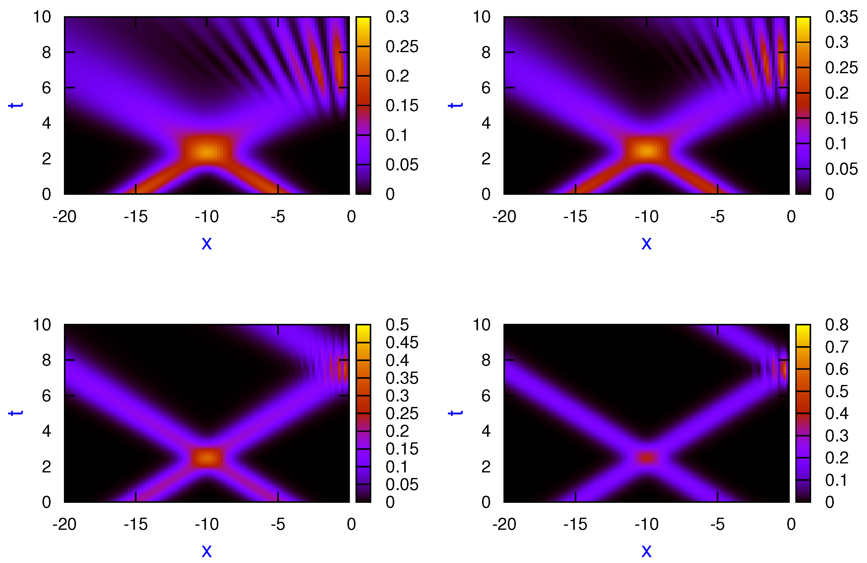
Figure 3.
A selection of scaled trajectories for the scaled pure (left column) and the scaled mixed state (right column) for the quantum regime (top panels) and the nearly classical regime (bottom panels). The same initial parameters are used as in previous figures.
Figure 3.
A selection of scaled trajectories for the scaled pure (left column) and the scaled mixed state (right column) for the quantum regime (top panels) and the nearly classical regime (bottom panels). The same initial parameters are used as in previous figures.
Figure 4.
Scaled arrival time distribution (43) at the detector location for the pure state (38) (left top panel) and the mixed state (39) (left bottom panel) for different regimes: (green curve), (red curve) and (black curve). Right top (bottom) panel depicts the scaled mean (uncertainty in) arrival time versus the transition parameter for the pure state (orange circled) and the mixed state (violet triangle up). The same initial parameters are used as in previous figures.
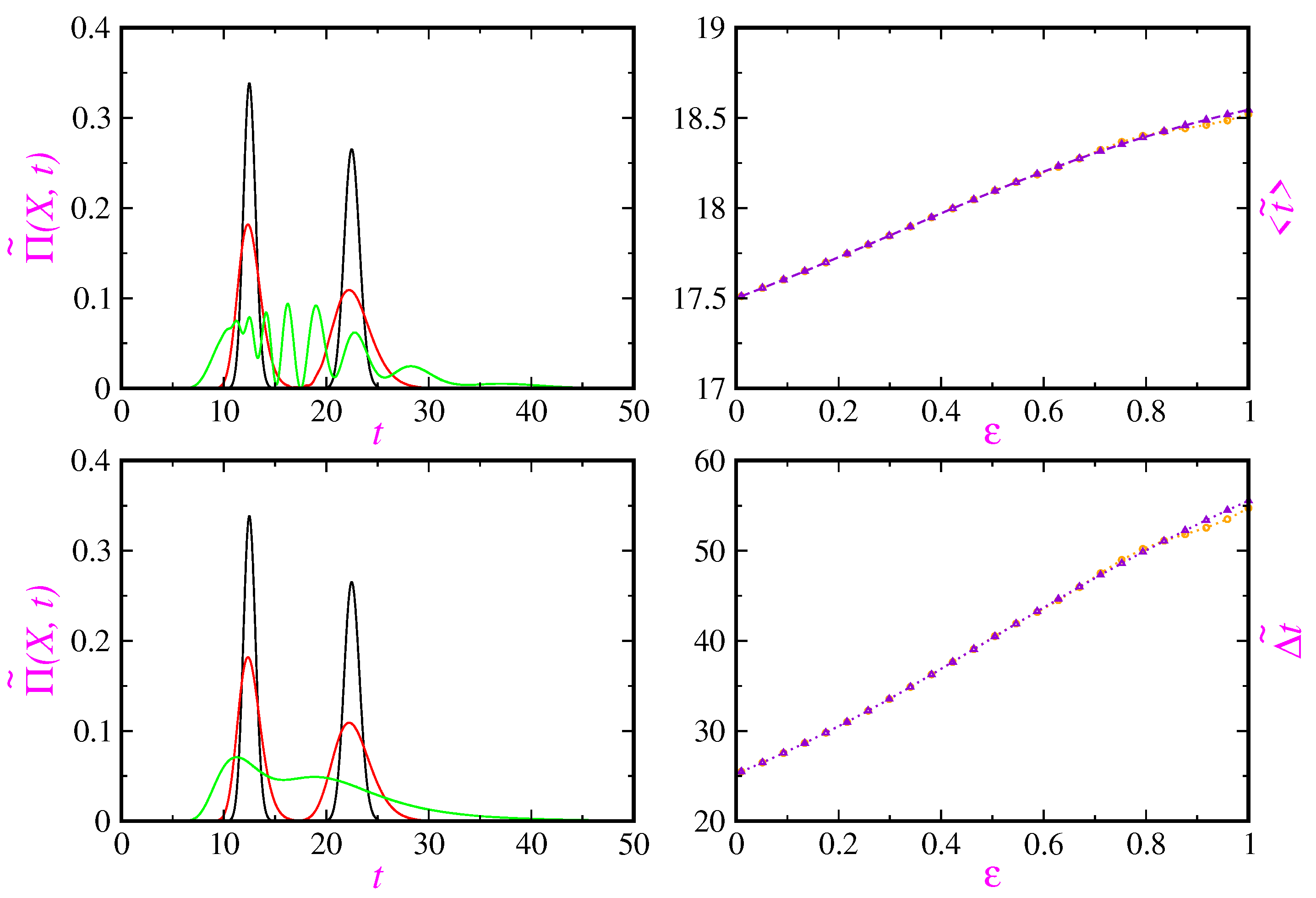
Figure 5.
Expectation value of position operator (left top panel), uncertainty in position (right top panel), expectation value of momentum operator (left bottom panel) and the product of uncertainties for the scaled mixed state for three different dynamical regimes: (green curves), (red curves) and (black curves). The same initial parameters are used as in previous figures.
Disclaimer/Publisher’s Note: The statements, opinions and data contained in all publications are solely those of the individual author(s) and contributor(s) and not of MDPI and/or the editor(s). MDPI and/or the editor(s) disclaim responsibility for any injury to people or property resulting from any ideas, methods, instructions or products referred to in the content. |
© 2023 by the authors. Licensee MDPI, Basel, Switzerland. This article is an open access article distributed under the terms and conditions of the Creative Commons Attribution (CC BY) license (http://creativecommons.org/licenses/by/4.0/).
Copyright: This open access article is published under a Creative Commons CC BY 4.0 license, which permit the free download, distribution, and reuse, provided that the author and preprint are cited in any reuse.


