
Submitted:
05 December 2023
Posted:
07 December 2023
You are already at the latest version
Abstract
In this study, we conducted a comprehensive analysis of the spatial distribution of soil organic carbon stock (SOC stock) and the associated uncertainties in two soil layers (0–10 cm and 0–30 cm; SOC stock 10 and SOC stock 30 respectively), in Valchiavenna, an alpine valley located in northern Italy . We employed the digital soil mapping (DSM) approach within different machine learning models, including multivariate adaptive regression splines (MARS), random forest (RF), support vector regression (SVR), and elastic net (ENET). Our dataset comprised soil data from 110 profiles, with SOC stock calculations for all sampling points based on bulk density (BD), whether measured or estimated, considering the presence of rock fragments. As environmental covariates for our research we utilized environmental variables, in particular geomorphometric parameters derived from a digital elevation model (with a 20 m pixel resolution), land cover data, and climat-ic maps. To evaluate the effectiveness of our models, we evaluated their capacity to predict SOC stock 10 and SOC stock 30 using the coefficient of determination (R2). The results for the SOC stock 10 were as follows: MARS 0.39, ENET 0.41, RF 0.69, and SVR 0.50. For the SOC stock 30, the corresponding R2 values were: MARS 0.45, ENET 0.48, RF 0.65, and SVR 0.62. Additionally, we calculated the Root Mean Square Error (RMSE) and Mean Absolute Error (MAE) for further assessment. To map the spatial distribution of SOC stock and address uncertainties in both soil layers, we chose the RF model, due to its better performance, as indicated by the highest R2 and the lowest RMSE and MAE. The resulting SOC stock maps using the RF model demonstrated an accuracy of RMSE = 1.35 kg.m-2 for the SOC stock 10 and RMSE= 3.36 kg.m-2 for the SOC stock 30. To further evaluate and illustrate the precision of our soil maps, we conducted an uncertainty assessment and mapping by analyzing the standard deviation (SD) from 50 iterations of the best-performing RF model. This analysis effectively highlighted the high accuracy achieved in our soil maps. The maps of uncertainty demonstrated that the RF model better predicts the SOC stock 10 compared to the SOC stock 30.
Keywords:
SOC stock
; DSM
; machine learning models
; uncertainty mapping
1. Introduction
Soil is an essential resource that offers numerous benefits for sustainable development, especially in the domains of food security and environmental regulation. One of its critical services is the storage of soil organic carbon (SOC), which is pivotal for both climate change mitigation and adaptation. Moreover, SOC plays a vital role in water management, enhancing soil capacity to address both floods and droughts[1,2] Poor soil management can lead to significant disruptions in soil parameters and characteristics, resulting in changes in SOC stocks. These changes, in turn, can cause the release of substantial amounts of carbon into the atmosphere. Sequestering carbon in the soil is a valuable method for controlling greenhouse gas levels in the atmosphere [3]. Studies indicate that this approach has the potential to capture approximately 0.8 to 1.5 billion metric tonnes of carbon annually. As a result, there is a high demand for accurate information and maps explaining the actual SOC stock and the soil's capacity for SOC sequestration [4].
Mountain ecosystems are characterized by a substantial amount of biological and cultural diversity, and they play a crucial role in providing essential services such as water and food security, and energy generation, as well as aesthetic and spiritual qualities [5]. According to the IPCC's WGII Sixth Assessment Report on Mountains [6], it is assumed that these ecosystems are extremely vulnerable to global changes. Mountainous soil is naturally vulnerable, and it is increasingly sensitive to changes in the environment [7]. Understanding the spatial distribution of SOC stocks in alpine mountains is essential for developing sustainable management strategies and environmental policies that can effectively address future global changes. However, this task remains difficult due to the complex morphology of these environments, which makes the collection of soil data challenging. Furthermore, comprehensive soil maps and information in the alpine mountains are scarce[8].In Italy, where a significant portion of the land area is covered by mountains, monitoring and assessment of the functionality of mountain soils becomes crucial. Detailed and accurate maps of SOC ensure that local and global decision-makers have access to precise information. From a pedological perspective, soils in the Italian Alps show diversity due to variations in factors related to pedogenesis[9]. These factors are associated with the differing landscape, including diverse climatic conditions, geological substrates, geomorphological processes, and the heterogeneity in land use and land cover (LU/LC)[10].
The development of geographic information systems (GIS), remote sensing, and mathematical algorithms have improved the techniques of digital soil mapping (DSM), which is suitable for mapping soil parameters in mountainous areas. In recent years, there has been a surge in studies that focus on mapping soil properties by applying various strategies such as geostatistics and machine learning [11]. These methodologies have sought to overcome the limitations of traditional methods, which are time-consuming and labor-intensive and cannot capture the real variability of soil properties in complex environments. The machine-learning models can be used to gain understanding of the complex interactions between soil properties and environmental factors and generate accurate predictions and maps [12]. In scientific research focused on SOC in alpine mountains, the primary approach involves examining the connections between SOC and environmental factors. These factors typically include topography, vegetation cover, and climate parameters, which serve as the main variables employed in DSM techniques. Yang et al. in 2016 employed boosted regression trees (BRT) and RF to model and map the SOC content of the Tibetan plateau. The two models showed good results, explaining about 70% of the SOC spatial distribution [13]; vegetation cover and the topographic variables were the most important covariates for SOC prediction. The mapping of SOC stock of several land cover types was carried out in the Bernese Alps, Switzerland, using different approaches [7]. The results of this research showed that, except for Regression Kriging, all interpolation approaches exhibited little variability in the RMSE of the expected SOC stock [7]. The spatial distribution of SOC stock in the Andossi plateau, Valchiavenna, was mapped at high-resolution using Regression Kriging with geomorphometric parameters. A detailed vegetation map was produced to improve the model's performance [14]. The geomorphometry influences soil formation and the storage of SOC in mountainous environments because it controls many factors of pedogenesis: for example, in the upper part of the slope, water and soil sediment (including organic matter) are lost without being compensated. On the other hand, at the foot of slopes, sediment inputs lead to soil accretion. Southern exposures are warmer and drier, and vegetation tends to be thermophilic or xerophilic, while northern exposures are colder [15]. This diversity of geomorphometric conditions influences the spatial distribution of soil properties; therefore, geomorphometry is a mandatory variable in DSM methodology. Most of the research cited [8,14] pointed out the need to enhance mapping methods to gather precise and comprehensive data on mountainous areas[1,16,17].
Uncertainty mapping is a critical step in the DSM approach, although it is not yet used in all DSM papers. Soil maps are a simplified representation of a more complex reality. As a result, no model is error-free, and no map is 100% accurate[18,19]. The causes of uncertainty in DSM are diverse: we may highlight four major sources of uncertainty: a) errors related to soil sampling and laboratory measurements; b) uncertainty of soil geospatial position measurement; c) uncertainties in covariate calculation; d) errors linked to modeling approaches. These lead to a number of errors in DSM outcomes. Statistical analyses of uncertainties and their mapping are strong tools for assessing map errors; they are critical for soil map users since they provide additional information about the error average that should be considered during the decision-making process[19,20,21].
The main objective of our research was to compare four machine learning models as DSM techniques, using geomorphometric and climatic variables and land cover as covariates, both i) to map the SOC stocks of two layers (0-10 cm: SOC stock 10, and 0-30 cm: SOC stock 30) and ii) to estimate the related uncertainties in an alpine valley.
2. Materials and Methods
2.1. Study area
Valchiavenna is a valley in the Central Alps, located in the province of Sondrio, Lombardy. It has a north-south orientation and is characterized by a varied landscape; the elevation changes from around 200 to 3279 m a.s.l. The morphology of the valley is linked to the action of water and glaciers, which acted at different times and in different ways. Glacial erosion is responsible for the transverse U-shaped profiles of the valley and its hanging sides. In addition, fluvial erosion forms have influenced and frequently re-shaped previous glacial morphologies. Valchiavenna has a considerable range of lithologies with crystalline-acidic character, mainly of metamorphic origin, and subordinately igneous rocks (late-Alpine Pluton intrusive body of Val Màsino and Val Bregaglia), as well as mesozoic cover and the group of mafic and ultramafic rocks (ophiolitic complex); in restricted areas (Pian dei Cavalli and the Andossi plateau) there are outcrops of sedimentary rocks of a carbonate type. According to the classification of climates by Köppen (1936), the climate of Valchiavenna is Cfb (humid temperate with maximum summer rainfall), with average annual precipitation in the range 1000–1400 mm. The average annual temperature in the valley bottoms is 12.8 °C, as measured by the Chiavenna meteorological station at 333 m a.s.l.; in the upper part of the valley, at Montespluga station (1908 m a.s.l.), the mean annual temperature drops to 2.7 °C. Valchiavenna has a high diversity in terms of vegetation and land use, from meadows and arable land in the lower parts to oak forests, coniferous forests, and finally alpine grasslands at high altitudes. Various soil types are present in the study area, categorized according to the classification system outlined in the World Reference Base for Soil Resources: Leptosols, Regosols, Cambisols, Umbrisols, Podzols and Histosols[22]. The soils in this study area are mostly coarse-textured (sandy loam; sometimes loam or loamy sand), often with a high content of rock fragments. In general, soil thickness ranges from 20 to 90 cm.
2.2. DSM approaches in SOC stock mapping
To achieve our objectives, we performed the following steps:
- soil survey and laboratory analyses;
- calculation of SOC stock at each sampling point;
- calculation and selection of environmental covariates;
- preparation of the covariate maps (with a spatial resolution of 20 x 20 m);
- extraction of the environmental covariates at each soil sampling point;
- selection of the covariates;
- comparison of different machine learning models to estimate the SOC stocks;
- spatialization of the SOC stocks;
- obtaining estimation uncertainty maps.
2.2.1. Soil survey and data collection strategy
The sampling was scattered across 18 topographic transects, chosen according to the physical nature of the study area. The main sampling transects were on the north-south axis, corresponding to the main orientation of Valchiavenna, and in transverse directions (generally east-west) along its secondary valleys (Figure 1). The position of each soil profile was chosen on the basis of elevation (approximately every 300 m). Since changes in altimetry across the topographic transects are associated with changes in the landscape (geomorphometry and vegetation), this sampling method provides an accurate representation of the valley landscape and its pedological variability. All the sampled soil profiles were georeferenced using a high-accuracy GPS. After the description of the profile, soil samples were collected from each horizon. At the end of the pedological survey, 110 soil profiles were described, for a total of 496 soil samples.
2.2.2. Laboratory analysis methods
The samples collected in the field were air-dried and sieved through a 2 mm sieve. The standard laboratory analyses were performed on the fine earth.
Soil pH was measured potentiometrically in a soil-to-water ratio of 1:2.5. The organic carbon was determined by oxidation with K2Cr2O7 in an acid environment (Walkley and Black, 1934); for samples very rich in organic matter (OM), we measured OM by incineration in a muffle furnace at 550 °C . A sieving and sedimentation method (pipette method; Burt 2004) was used to obtain textural fractions: coarse sand (2.0-0.1 mm), fine sand (0.1-0.05 mm), silt (0.05-0.002 mm), and clay (<0.002 mm).
As the main objective of this work was to map the SOC stock by soil layers, the calculation per unit area was carried out as follows: from the per-horizon data, the SOC content and that of the rock fragments (described in the field) of each soil layer was calculated; then the bulk density (BD, g cm-3) of each layer was estimated using pedotransfer functions (unpublished) obtained in a detailed study of soils on the Andossi plateau (upper Valchiavenna). BD1 and BD2 (equation 2 and 3) represent the BD of layer 0-10 cm and 10-30 cm, respectively. After obtaining these data, we calculated the SOC stock of each soil layer using equation 1.
2.2.3. Environmental covariates
The environmental variables used as covariates are illustrated in Table 1. The covariates were calculated with different methodologies and transferred to raster layers with a 20-m spatial resolution in a GIS environment, using the open-source software QGIS 3.16.1. We used three different types of environmental covariates: geomorphometric, climatic, and land cover.
- Geomorphometric covariates: to calculate these covariates we used the digital terrain model (DTM), delivered from the regional geo-portal of Lombardy (www.geoportale.regione.lombardia.it), and extracted 16 morphometric parameters. The calculation was carried out in QGIS 3.16.1 using the integrated SAGA tool.
- Climatic covariates: we used mean annual air temperature (T) and precipitation (P) delivered from WorldClim (www.worldclim.org) with spatial resolution of 1 km2. We applied a statistical downscaling technique using a 30-year time series of climatic data registered at seven meteorological stations in Valchiavenna, to obtain climatic covariate maps with the same spatial resolution as the other environmental variables (20 m). Working in an alpine valley, the downscaling technique was based on statistical correlations between climatic variables with the elevation and also with latitude and longitude [23]. The results of the correlations were used to obtain T and P maps of the area, correcting the estimated values for slope and exposure, which have a direct impact on microclimatic conditions in mountainous environments [24]. The equations used for climate downscaling are explained in the Supplementary materials (Eq S1 - Eq S5).
- Land cover covariates: we used the most recent land cover maps of Lombardy, related to agricultural and forestry use (DUSAF 7.0) [25] and identified six land cover classes in the study area: broadleaf forests, coniferous forests, grasslands (low elevation), prairies (high elevation), peatlands, and rocky soils.
2.2.4. Covariates selections and modeling approaches
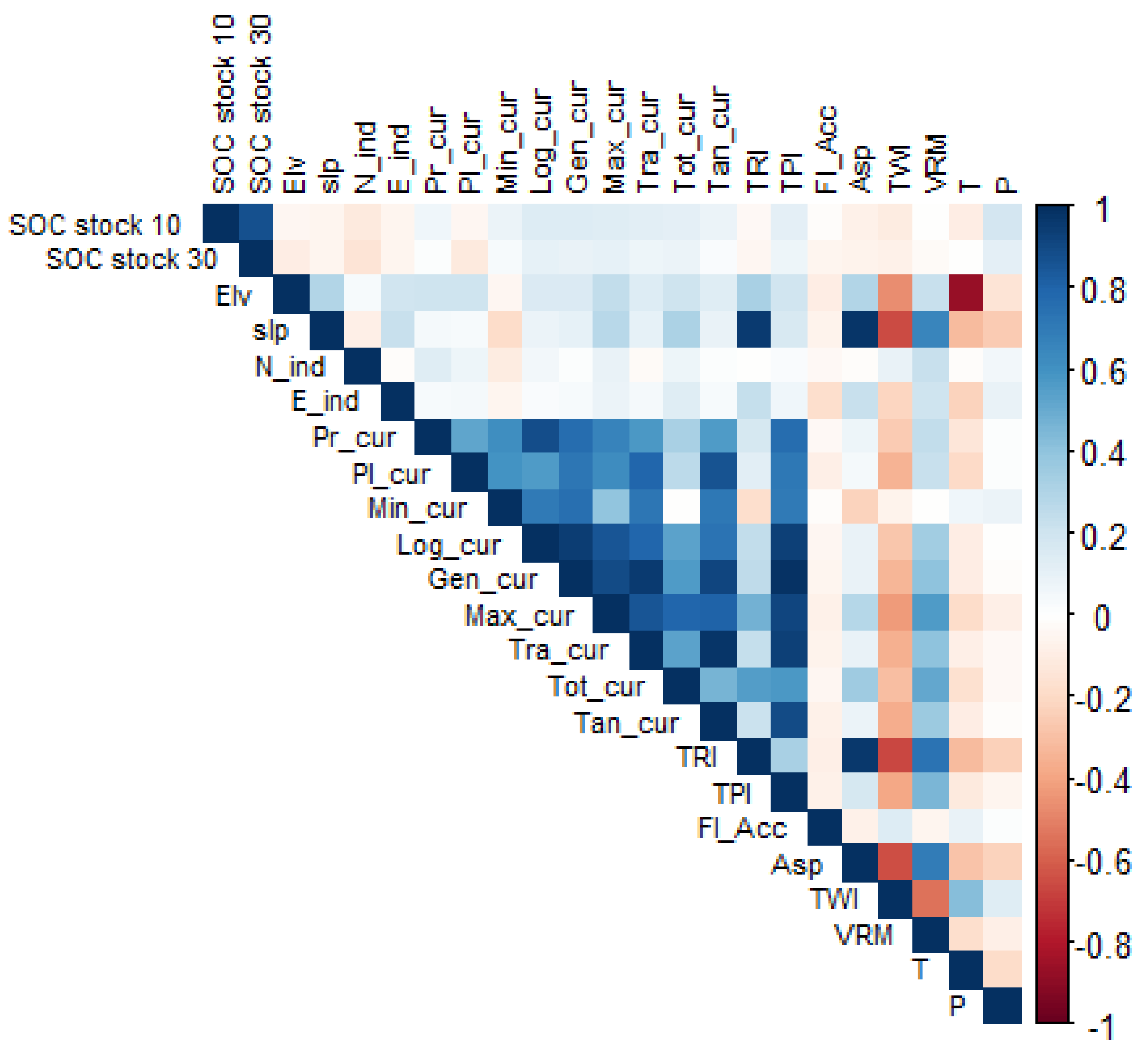
We used the variables selection strategy, which is a mandatory step in DSM, to improve the models’ performance and guard against noise and overfitting problems. Firstly, we created a correlation matrix between the different continuous variables, one of each of highly correlated pair was reduced (correlation coefficient >0.8); all the categorical variables (land cover) were used in the modeling.
To understand the differences in the distribution of SOC stock according to the land cover, we used the one-way ANOVA with the post hoc Tukey HSD test (Tables S1 and S2). The statistical analysis and modeling were performed using R software (R Development Core Team, 2021). For the DSM approach, we built different machine learning models: MARS, ENET, RF, and SVR using "Caret" and "Train" packages of the R software to fit the different models. We also applied hyperparameter tuning to automatically select the best model structures according to the lowest predictions errors. We applied data standardization to models (SVR and ENET) that require this preprocessing step.
- Multivariate Adaptive Regression Splines (MARS). In 1991, Friedman unveiled a new methodology that amalgamated linear regression with spline mathematical modeling through binary recursive partitioning [26]. This method constructs a model step by step, assessing variable importance and regularization to unimportant covariates. MARS is flexible, identifying complex nonlinear interactions between input variables, and it requires minimal pre-processing. Until now, the MARS model has not been widely applied in soil properties prediction [27,28].
- Elastic Net Model (ENET). The model was introduced by Zou and Hastie in 2005 [29]. Similar to Lasso and Ridge Regression, it employs a regulation and variable selection technique, choosing the most advantageous combination of the two models. For studies with few observations and a high number of predictors, it is advised to use this model [29,30,31].
- Random Forests (RF). Proposed by Breiman in 2001 [32], RF is the most used machine learning algorithm in DSM, as it has proven effective in mapping soil properties over an extensive variety of data sources and scales of soil heterogeneity. The model uses decision trees for training, combining them to produce single predictions for each observation in the datasets using an out-of-bag (OOB) strategy [33].
- Support Vector Machine (SVM). An effective machine learning method for mapping soil properties, largely used by soil mappers in recent years [34,35]; it is a kernel-based model, highly used to analyze non-linear relationships over a high-dimensional induced feature space. SVM uses decision surfaces specified by a kernel function [36]. In the DSM approach, SVM is frequently used for classification, but it is also used for regression predictions.
2.2.5. Prediction validation and uncertainties mapping
A 10-fold cross-validation was employed to assess the model. In DSM, cross-validation is frequently employed since it splits the data into several training and test datasets. Moreover, it is advisable to utilize the cross-validation technique when conducting studies in regions where data collection is limited, such as mountainous areas [37,38]. We employed the following metrics to validate the models: the mean absolute prediction error (MAE), the root means square error (RMSE) and the coefficient of determination (R2). To map the uncertainties we used the standard deviation (SD) of 50 runs, as proposed by the Global Map Project [19,20,33]; in addition the zonal statistics was applied to understand the uncertainty distribution under the different land cover types.
3. Results
3.1. SOC stock statistical analysis
The SOC stock values at 10 and 30 cm soil layers are summarized in Table 2. The results illustrate that the soils in our study area store a significant amount of SOC, especially in the top 30 cm, where the average is 8.72 kg m-2. The mean SOC stock for 30 cm is approximately twice as high as that for 10 cm, which averaged 4.29 kg m-2. The standard SD results reveal a high variability in the SOC stock data, indicating a high spatial heterogeneity in the distribution of SOC stock in our study area. This is a result of the high pedo-diversity characterizing the Valchiavenna valley.
The correlation matrix of the SOC stock with the covariates used is shown in Figure 2. Many variables are highly correlated, as for example temperature and elevation. Notably, parameters such as Pl_cur, Max_cur and TPI exhibit significant correlations. Additionally, climatic factors such as T and P are shown to exert control over the SOC stock. It's important to note that while the Pearson correlation coefficient indicates this relationship, its capacity to explain the complex statistical dynamics of the relationship between SOC stock and the environmental parameters remains limited.
Figure 2.
Correlation matrix of SOC stock and the variables used as environmental covariates.
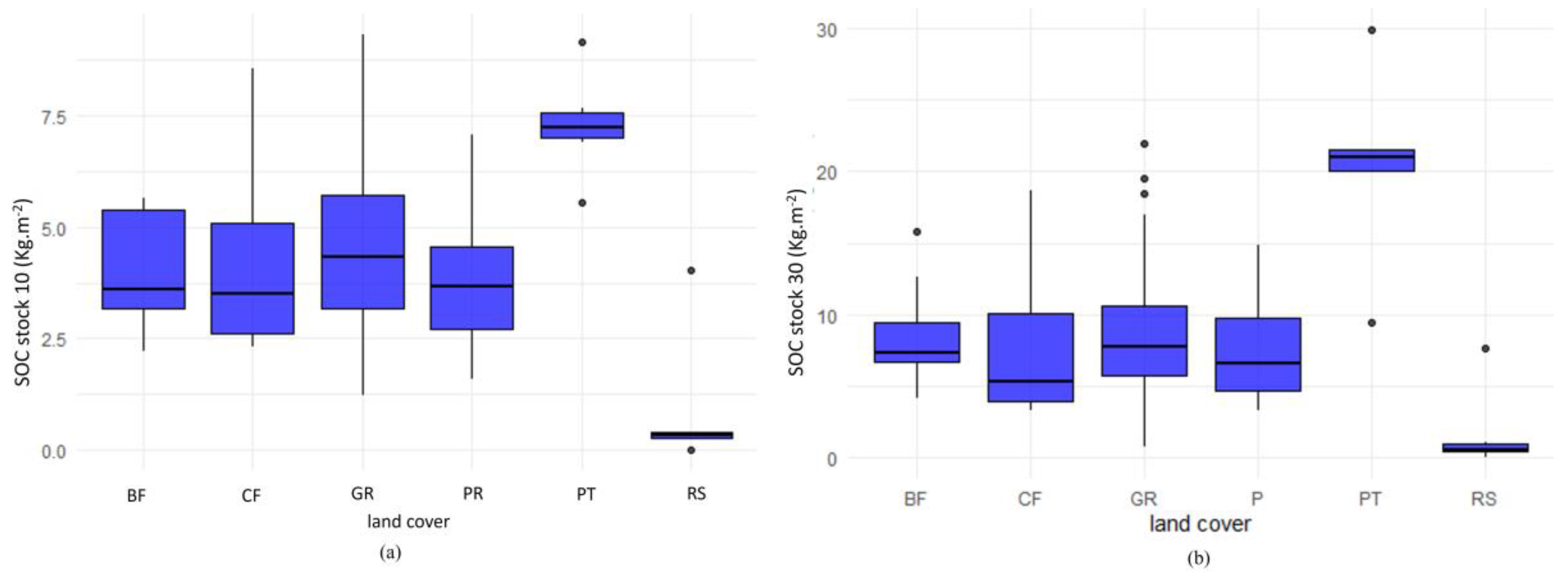
The boxplot of the distribution of SOC stock by land cover types (Figure 3) shows that by far the highest SOC storage is found in peatlands, while the lowest is found in high altitude, thin and skeletal soils. In the other cases, SOC storage is comparable, but that of soils in coniferous forests is on average lower than that of broadleaf forests and natural or cultivated grasslands. The results of the ANOVA analysis confirm this statistically: Tukey's HSD test shows that the greatest differences are found between rocky soils and peatlands (Tables S1 and S2).
Figure 3.
Boxplot of SOC stock distribution by different land cover types (BF: Broadleaf forests; CF: Coniferous forests; GR: Grasslands; PR: Prairies; PT: Peatlands; RS: Rocky soils): (a) SOC stock 0-10 cm; (b) SOC stock 0-30 cm. The boxplots represent the following metrics: the median first and third quantile (Q1, Q3), maximum, minimum values and outliers.
3.2. Models validation and SOC stock prediction
The model validation results, obtained from the average of 50 training trials of the models, are shown in Table 3. For both soil layers the RF model demonstrated the best validation results, with the highest R2 and the lowest RMSE and MAE. However, the errors of SOC stock prediction are higher for the SOC stock 30 (MAE=2.48 kg.m-2), compared to the SOC stock 10 (MAE=1.10 kg.m-2).
The SVR model also showed good results, better than for ENET and MARS, which were almost equal in performance.
The results showed that the RF model performed well in predicting SOC stock in both soil layers, with particularly good results in the 0-10 cm compared to the 0-30 cm layer. When we compared MAE with the average SOC stock values (0-10 cm: 4.29 kg m-2, 0-30 cm: 8.72 kg m-2), the RF model displayed a 26% error rate for SOC stock at 10 cm and a 28% error rate for SOC stock at 30 cm. Interestingly, the SVR consistently showed higher results of MAE comparing to the RF model.
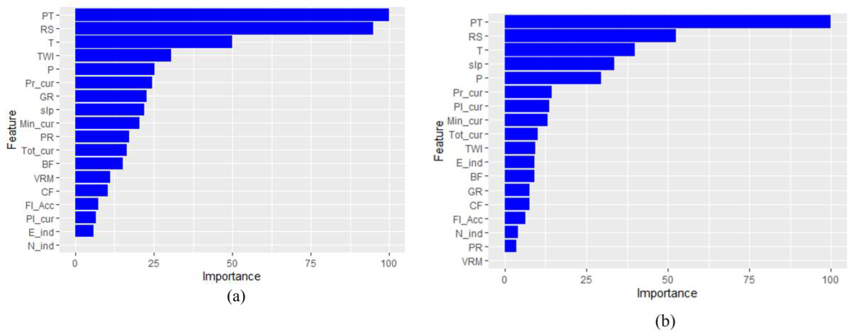
The order of importance of the predictors (Figure 3 and supplementary material) changes from one model to another, depending on the type of model and its structure. The MARS and ENET models used fewer variables than RF and SVR. In the RF model, land cover was the most important predictor, followed by climate parameters and several geomorphometric variables (mainly curvatures).
Figure 3.
Predictors importance of SOC stock mapping using RF model (CF: Coniferous forests; PR: Prairies; GR: Grasslands; BF: Broadleaf forests; RS: Rocky soils; PT: Peatlands): (a) SOC stock 0-10 cm; (b) SOC stock 0-30 cm.
Figure 3.
Predictors importance of SOC stock mapping using RF model (CF: Coniferous forests; PR: Prairies; GR: Grasslands; BF: Broadleaf forests; RS: Rocky soils; PT: Peatlands): (a) SOC stock 0-10 cm; (b) SOC stock 0-30 cm.
3.3. Maps of SOC stock and uncertainty estimation
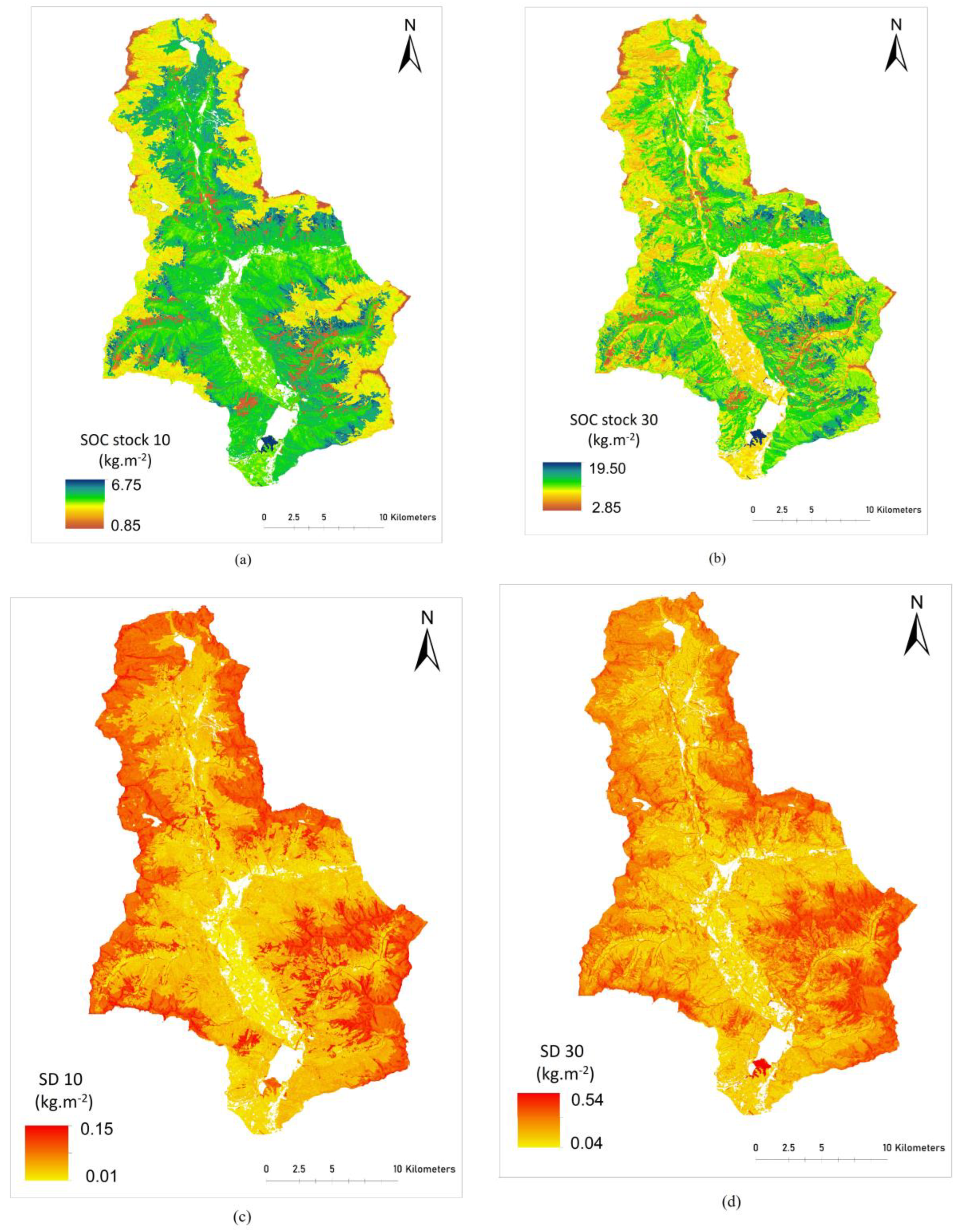
We employed the RF model to represent the spatial distribution of SOC stock and the associated uncertainties (Figure 5) since it produced the best prediction results (Table 3).
The prediction maps of SOC stocks show a similarity in the spatial pattern of the two soil layers considered. The central region of the valley has a higher storage of organic carbon: these are areas covered by broadleaf forests, coniferous forests, and grasslands, located at medium altitudes. The lowest values correspond to high-altitude and sloping areas, where the vegetation is sparse, and the soil is thin and rich in rock fragments. The valley floor areas show a different behavior: for the 0-10 cm layer they have stock values comparable to those of the forest areas, while for the 0-30 cm they have significantly lower stockage. This is because the soils on the valley floor are managed as grassland, alternating with arable land: these are soils in which there is a fair level of organic matter in the surface horizon, while at depth the content decreases considerably. The value of the SOC stock, estimated cartographically, is obviously greater for the 0-30 cm layer (2.9 to 19.5 kg m-2) than for the 0-10 cm layer (0.8 to 6.8 kg m-2).
The maps displaying the uncertainty (obtained as the variance from 50 repetitions of the estimates) of SOC stock 10 has a range between 0.01 and 0.15 kg m-2. For SOC stock 30 the error varies between 0.04 and 0.54 kg m-2. These results indicate that there are generally low levels of uncertainty, underscoring the model’s stability.
A statistical analysis of the uncertainty distribution across different land cover types, as shown in Figure 4, reveals that errors in SOC stock predictions tend to be higher at elevated altitudes, especially in areas with significant slopes and rocky soils.
Figure 4.
Average of SOC stock uncertainty distribution under different land cover types (CF: Coniferous forests; PR: Prairies; GR: Grasslands; BF: Broadleaf forests; RS: Rocky soils; PT: Peatlands).
Figure 4.
Average of SOC stock uncertainty distribution under different land cover types (CF: Coniferous forests; PR: Prairies; GR: Grasslands; BF: Broadleaf forests; RS: Rocky soils; PT: Peatlands).
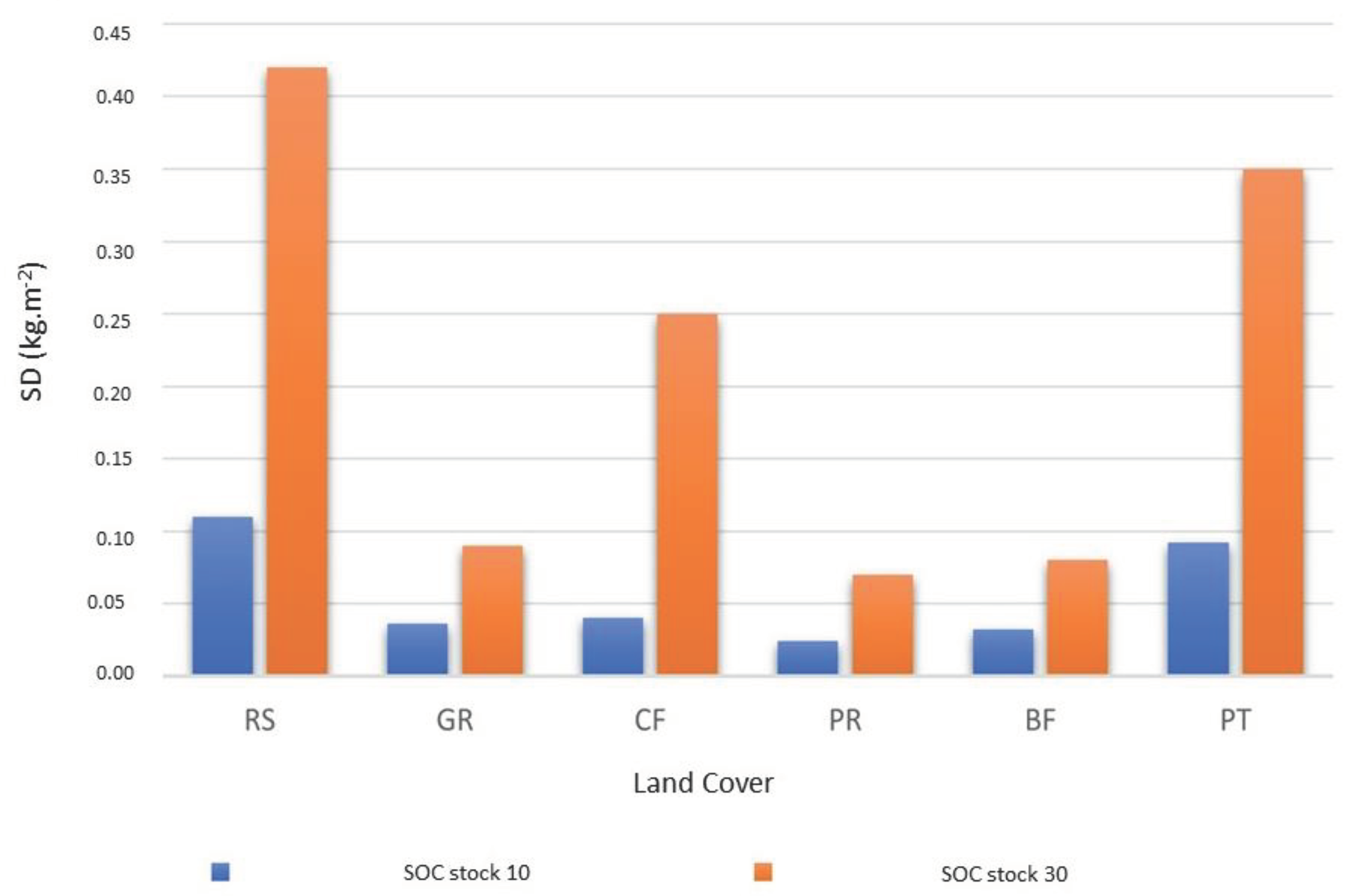
Figure 5.
Maps of SOC stock and associated uncertainties in Valchiavenna: (a) SOC stock 10 distribution map; (b) SOC stock 30 distribution map; (c) uncertainty map for SOC stock 10 (SD 10); (d) uncertainty map for SOC 30 (SD 30).
Figure 5.
Maps of SOC stock and associated uncertainties in Valchiavenna: (a) SOC stock 10 distribution map; (b) SOC stock 30 distribution map; (c) uncertainty map for SOC stock 10 (SD 10); (d) uncertainty map for SOC 30 (SD 30).
4. Discussion
4.1. Models’ performance
The performance of machine learning models can vary because each model operates differently, due to its unique structure. The choice of variables, which differs from model to model, has a significant impact on how well the model performs. For instance, in the MARS model, which gave the least accurate predictions, only a few variables were chosen, resulting in a loss of information about the relationship between SOC stock and environmental factors. In contrast, RF and SVR used a more extensive set of variables, leading to much better model performance. Our research obtained results consistent with previous scientific work on predicting and mapping soil properties such as SOC stock, demonstrating the robust performance of the RF model. In complex tropical landscapes, RF rivalled the predicting power of the boosted regression tree (BRT) algorithm, skillfully handling data variability and mitigating irrelevant factors [39]. Similarly, in a study using Sentinel-1 and Sentinel-2 for soil mapping, RF competed effectively among machine learning methods for SOC prediction, highlighting its promise when coupled with multi-source sensor data [40]. In a study focused on employing machine learning for SOC prediction in agriculture, XGBoost demonstrated exceptional accuracy. In the same study the RF model also performed admirably. Furthermore, the integration of Sentinel-1 and Sentinel-2 data significantly enhanced the precision of these predictions [41]. Another research project focused on predicting SOC content using RF, k-nearest neighbors (kNN), SVM, artificial neural network (ANN), and ensembles. RF stood out, with excellent predictive performance [42]. Similarly, the work of Zhang et al. (2022) aims to map the SOC distribution in China using machine learning; when comparing models, RF emerged as superior, with higher R2 and lower RMSE values across soil depths (0-10, 10-20, 20-30, and 30-40 cm) [31].
4.2. SOC stock spatial distribution: the main drivers and uncertainties
The results of the RF model show that the main environmental drivers of SOC stocks in Valchiavenna are land cover types, climate and geomorphometric variables (slope, curvatures and TWI). These results are in agreement with previous studies [16,17], which have shown that SOC stocks in mountain environments are strongly influenced by vegetation cover and climatic conditions.
Previous research has shown that the type of land cover and habitat significantly influences the storage of SOC stock in alpine mountains. Consequently, the type of vegetation is a crucial parameter because it directly impacts the storage of organic carbon in the soil [43]. Our results illustrate that peatlands, grasslands, and coniferous forests can store considerably more carbon in the soil compared to broadleaf forests and prairies. Our results also show that the SOC stock is significantly influenced by climatic conditions. Air temperature has a strong influence as it controls the rate of mineralization of organic matter in the SOC balance and therefore affects the output rate. In alpine ecosystems, SOC stocks increase with altitude, at least beyond the belt of natural grasslands, where thin and rocky soils have only sparse and discontinuous vegetation, so there is a negative relationship between temperature and SOC storage [44]. As a result of ongoing climate change, increases in temperature are therefore expected to reduce SOC storage. Mitigation measures favoring carbon sequestration strategies (protection or restoration of peatlands, afforestation, sustainable grassland cultivation, etc.) should focus on the most fragile mountain ecosystems [43,45]. Precipitation also controls the dynamics of SOC storage in mountain soils: it is essential for net primary production (NPP) and has an impact on soil moisture, pH and respiration [46].
However, research assessing the impact of changes in precipitation on the soil SOC budget is still limited[46,47]. Geomorphometric and topographic factors have an important influence on SOC stock spatial distribution, although their impact is generally less significant than climatic factors. The importance of geomorphometrical predictors on the spatial distribution of SOC stock differs between the top 10 cm and the top 30 cm of soil. For example, Figure 3 illustrates that the wetness index has a more notable effect on SOC stock distribution in the upper 10 cm compared to the upper 30 cm, as it influences the soil water content, which influences directly the SOC stock. Slope and aspect control the solar radiation and soil moisture: steeper slopes often experience higher rates of erosion, which can result in reduced soil development and SOC storage; aspect influences the exposure to sunlight, affecting vegetation growth and decomposition rates, which, in turn, impact SOC accumulation. The landforms, such as the curvatures, control the zones of SOC erosion and deposition. Previous research has already demonstrated the relationship between SOC stock variability and geomorphometry [17,35,48].
By examining the maps, it appears that there is a correlation between topographical parameter attributes and prediction errors. Higher altitudes with significant slopes and rocky soils exhibit greater prediction errors, particularly in regions with complex topography and shallow soils prone to erosion. In contrast, valleys and low-lying areas display lower uncertainties due to their uniform soils and agricultural land use. Peatlands stand out with notably increased uncertainty, especially for SOC stock 30. This is attributed to the limited number of peatland soils sampled and to the variability of their soil characteristics in our study area. Further, the analysis of uncertainty distribution by land use indicates a threefold higher uncertainty in predicting SOC stock 30 compared to SOC stock 10. This underscores the complexity of the SOC stock prediction and highlights the need for more data acquisition and model calibration.
It is essential to note that when comparing the SOC stock ranges depicted in the final maps with those observed in the actual data, a noticeable trend emerges. The RF model appears to impose a limitation on the SOC stock range. For instance, in the observed dataset, the SOC stock 10 spans from 0.02 to 9.31 kg m-2; however, in the generated map, this range contracts to 0.85 to 6.75 kg m-2. Similarly, examining the SOC stock 30, in the map the range shifts from 2.85 to 19.50 kg m-2, while in the observed data it increases from 0.03 to 29.90 kg m-2. The differences in SOC stock ranges between the model's maps and the actual data highlight the fact that the model does not perform perfectly for soils with very high or very low SOC stock amounts. This mismatch in accuracy is due to several factors that are partly, not solely, due to the modeling process. The complicated mountain landscape makes the modeling harder, and the difficulties in collecting data in this area make the challenges higher. The complex terrain and the problems with getting representative samples both contribute to this issue. The SOC stock uncertainty maps reveal insights into predictive accuracy across diverse land covers and depths. These findings contribute to our understanding of carbon dynamics and underscore challenges in modeling complex terrains and unique land covers. Our research demonstrates that the Valchiavenna stocks a high amount of SOC: this means that the soils of this valley provide important ecosystem services that should be taken in consideration to mitigate and adapt the impact of climate change and that it is necessary to manage soils carefully and protect them from degradation, to avoid the loss of SOC, especially under climatic change scenarios.
5. Conclusions
The machine learning models applied in our research showed different performances, which is important in the context of DSM approaches to better understand the suitable modelling techniques. The RF model showed the best performance results compared to the other models. The results highlight the crucial role that machine learning models play in accurately capturing the complex relationships between SOC stock and environmental factors. Our research indicates that land cover and climatic factors are the most important predictors of SOC stock spatial distribution; geomorphometric parameters (slope, curvatures and TWI) also demonstrated a significant impact in our mountainous environments.
The future development of this work may involve enhancing data collection in areas where uncertainties are great: the precision and accuracy of the output's maps might be improved by a future data-gathering design for models’ validation. Using additional predictors such as parent material maps and the history of the land use may also improve the quality of maps. The use of future projection scenarios of climate and land use changes would be a way to include temporal data to enhance knowledge of SOC dynamics over time in this environment, for the adoption of sustainable land management strategies. Therefore, the next step of this work is the prediction of SOC stocks under future climate change scenarios using machine learning and climatic models. This study contributes to the understanding of SOC dynamics and mapping at a local scale: the knowledge of SOC stocks can be used by decision-makers to protect regions with high actual carbon storage potential, such as mountain forests, peatlands and grasslands, or zones at high risk of losing SOC stock, such as the upper belts of the valley. Finally, our research offers valuable information into the distribution of soil organic carbon stock in mountainous areas and can be used to assess ecosystem services, environmental management strategies, and support plans to mitigate climate change in these areas.
References
- Baruck, J. et al. Soil classification and mapping in the Alps: The current state and future challenges. Geoderma 264, 312–331 (2016). [CrossRef]
- Romeo, R. et al. Understanding Mountain Soils: A contribution from mountain areas to the International Year of Soils 2015. https://iris.unito.it/handle/2318/1522121 (2015).
- Hartemink, A. E., Gerzabek, M. H., Lal, R. & McSweeney, K. Soil Carbon Research Priorities. in Soil Carbon (eds. Hartemink, A. E. & McSweeney, K.) 483–490 (Springer International Publishing, 2014). [CrossRef]
- Lal, R. et al. The carbon sequestration potential of terrestrial ecosystems. J. Soil Water Conserv. 73, 145A-152A (2018). [CrossRef]
- Alfthan, B. et al. Mountain Adaptation Outlook Series: Synthesis Report. (2018).
- Adler, C., P., Weste, I., Bhatt, C. & Huggel. Climate Change 2022 – Impacts, Adaptation and Vulnerability: Working Group II Contribution to the Sixth Assessment Report of the Intergovernmental Panel on Climate Change. (Cambridge University Press, 2023). [CrossRef]
- Hoffmann, U., Hoffmann, T., Jurasinski, G., Glatzel, S. & Kuhn, N. J. Assessing the spatial variability of soil organic carbon stocks in an alpine setting (Grindelwald, Swiss Alps). Geoderma 232–234, 270–283 (2014). [CrossRef]
- Lagacherie, P. & McBratney, A. B. Chapter 1 Spatial Soil Information Systems and Spatial Soil Inference Systems: Perspectives for Digital Soil Mapping. in Developments in Soil Science vol. 31 3–22 (Elsevier, 2006).
- D’Amico, M. E., Freppaz, M., Leonelli, G., Bonifacio, E. & Zanini, E. Early stages of soil development on serpentinite: the proglacial area of the Verra Grande Glacier, Western Italian Alps. J. Soils Sediments 15, 1292–1310 (2015). [CrossRef]
- D’Amico, M. E., Freppaz, M., Filippa, G. & Zanini, E. Vegetation influence on soil formation rate in a proglacial chronosequence (Lys Glacier, NW Italian Alps). CATENA 113, 122–137 (2014). [CrossRef]
- Wang, D. et al. Modeling soil organic carbon spatial distribution for a complex terrain based on geographically weighted regression in the eastern Qinghai-Tibetan Plateau. CATENA 187, 104399 (2020). [CrossRef]
- Ferré, C., Caccianiga, M., Zanzottera, M. & Comolli, R. Soil–plant interactions in a pasture of the Italian Alps. J. Plant Interact. 15, 39–49 (2020). [CrossRef]
- Yang, R.-M. et al. Comparison of boosted regression tree and random forest models for mapping topsoil organic carbon concentration in an alpine ecosystem. Ecol. Indic. 60, 870–878 (2016). [CrossRef]
- Ballabio, C., Fava, F. & Rosenmund, A. A plant ecology approach to digital soil mapping, improving the prediction of soil organic carbon content in alpine grasslands. Geoderma 187–188, 102–116 (2012). [CrossRef]
- Baize, D. Naissance et évolution des sols : La pédogenèse expliquée simplement. 1–160 (2021).
- Dorji, T., Odeh, I. O. A., Field, D. J. & Baillie, I. C. Digital soil mapping of soil organic carbon stocks under different land use and land cover types in montane ecosystems, Eastern Himalayas. For. Ecol. Manag. 318, 91–102 (2014). [CrossRef]
- Li, Y. et al. Effects of land use and land cover change on soil organic carbon storage in the Hexi regions, Northwest China. J. Environ. Manage. 312, 114911 (2022). [CrossRef]
- Vaysse, K. & Lagacherie, P. Using quantile regression forest to estimate uncertainty of digital soil mapping products. Geoderma 291, 55–64 (2017). [CrossRef]
- Heuvelink, G. Uncertainty quantification of GlobalSoilMap products. Glob. Basis Glob. Spat. Soil Inf. Syst. - Proc. 1st Glob. Conf. 335–340 (2014). [CrossRef]
- Peralta, G., Di Paolo, L. & Luotto, I. Global Soil Organic Carbon Sequestration Potential Map – GSOCseq v.1.1. (FAO, 2022). [CrossRef]
- Nations, Y., Olmedo, G. F. & Reiter, S. Soil Organic Carbon Mapping Cookbook 2nd Edition. (2018).
- IUSS Working Group WRB. World Reference Base for Soil Resources. (2022).
- Bc, H. & Rg, C. Climate downscaling: techniques and application. Clim. Res. 07, 85–95 (1996).
- Belloni, S. & Pelfini, M. Il gradiente termico in Lombardia, Dipartimento di scienze terra del università di Milano. Acqua-Aria 4, 441–447 (1987).
- DUSAF 7.0 - Uso e copertura del suolo 2023 - Geoportale della Lombardia. https://www.geoportale.regione.lombardia.it/news/-/asset_publisher/80SRILUddraK/content/dusaf-7.0-uso-e-copertura-del-suolo-2023.
- Friedman, J. H. Estimating Functions of Mixed Ordinal and Categorical Variables Using Adaptive Splines. https://apps.dtic.mil/sti/citations/ADA590939 (1991).
- Rentschler, T. et al. Comparison of catchment scale 3D and 2.5D modelling of soil organic carbon stocks in Jiangxi Province, PR China. PLOS ONE 14, e0220881 (2019). [CrossRef]
- Wang, L.-J., Cheng, H., Yang, L.-C. & Zhao, Y.-G. Soil organic carbon mapping in cultivated land using model ensemble methods. Arch. Agron. Soil Sci. 68, 1711–1725 (2022). [CrossRef]
- Zou, H. & Hastie, T. Regularization and Variable Selection Via the Elastic Net. J. R. Stat. Soc. Ser. B Stat. Methodol. 67, 301–320 (2005). [CrossRef]
- Sirsat, M. S., Cernadas, E., Fernández-Delgado, M. & Barro, S. Automatic prediction of village-wise soil fertility for several nutrients in India using a wide range of regression methods. Comput. Electron. Agric. 154, 120–133 (2018). [CrossRef]
- Zhang, J., Schmidt, M. G., Heung, B., Bulmer, C. E. & Knudby, A. Using an ensemble learning approach in digital soil mapping of soil pH for the Thompson-Okanagan region of British Columbia. Can. J. Soil Sci. 102, 579–596 (2022).
- Breiman, L. Random Forests. Mach. Learn. 45, 5–32 (2001).
- Wadoux, A. M. J.-C., Minasny, B. & McBratney, A. B. Machine learning for digital soil mapping: Applications, challenges and suggested solutions. Earth-Sci. Rev. 210, 103359 (2020). [CrossRef]
- Khaledian, Y. & Miller, B. A. Selecting appropriate machine learning methods for digital soil mapping. Appl. Math. Model. 81, 401–418 (2020). [CrossRef]
- Were, K., Bui, D. T., Dick, Ø. B. & Singh, B. R. A comparative assessment of support vector regression, artificial neural networks, and random forests for predicting and mapping soil organic carbon stocks across an Afromontane landscape. Ecol. Indic. 52, 394–403 (2015). [CrossRef]
- Cortes, C. & Vapnik, V. Support-vector networks. Mach. Learn. 20, 273–297 (1995).
- Piikki, K., Wetterlind, J., Söderström, M. & Stenberg, B. Perspectives on validation in digital soil mapping of continuous attributes—A review. Soil Use Manag. 37, 7–21 (2021). [CrossRef]
- Tajik, S., Ayoubi, S. & Zeraatpisheh, M. Digital mapping of soil organic carbon using ensemble learning model in Mollisols of Hyrcanian forests, northern Iran. Geoderma Reg. 20, e00256 (2020). [CrossRef]
- Ließ, M., Schmidt, J. & Glaser, B. Improving the Spatial Prediction of Soil Organic Carbon Stocks in a Complex Tropical Mountain Landscape by Methodological Specifications in Machine Learning Approaches. PLOS ONE 11, e0153673 (2016).
- Zhou, T. et al. High-resolution digital mapping of soil organic carbon and soil total nitrogen using DEM derivatives, Sentinel-1 and Sentinel-2 data based on machine learning algorithms. Sci. Total Environ. 729, 138244 (2020). [CrossRef]
- Nguyen, T. T. et al. A novel intelligence approach based active and ensemble learning for agricultural soil organic carbon prediction using multispectral and SAR data fusion. Sci. Total Environ. 804, 150187 (2022). [CrossRef]
- Zeraatpisheh, M., Ayoubi, S., Mirbagheri, Z., Mosaddeghi, M. R. & Xu, M. Spatial prediction of soil aggregate stability and soil organic carbon in aggregate fractions using machine learning algorithms and environmental variables. Geoderma Reg. 27, e00440 (2021). [CrossRef]
- Yigini, Y. & Panagos, P. Assessment of soil organic carbon stocks under future climate and land cover changes in Europe. Sci. Total Environ. 557–558, 838–850 (2016). [CrossRef]
- Ma, M. & Chang, R. Temperature drive the altitudinal change in soil carbon and nitrogen of montane forests: Implication for global warming. CATENA 182, 104126 (2019). [CrossRef]
- Odebiri, O. et al. Estimating soil organic carbon stocks under commercial forestry using topo-climate variables in KwaZulu-Natal, South Africa. South Afr. J. Sci. 116, 1–8 (2020).
- Parton, W. j. et al. Impact of climate change on grassland production and soil carbon worldwide. Glob. Change Biol. 1, 13–22 (1995). [CrossRef]
- Puche, N. J. B., Kirschbaum, M. U. F., Viovy, N. & Chabbi, A. Potential impacts of climate change on the productivity and soil carbon stocks of managed grasslands. PLOS ONE 18, e0283370 (2023). [CrossRef]
- Chen, S. et al. A high-resolution map of soil pH in China made by hybrid modelling of sparse soil data and environmental covariates and its implications for pollution. Sci. Total Environ. 655, 273–283 (2019). [CrossRef]
Figure 1.
Geographical position of the study area and soil profile location.
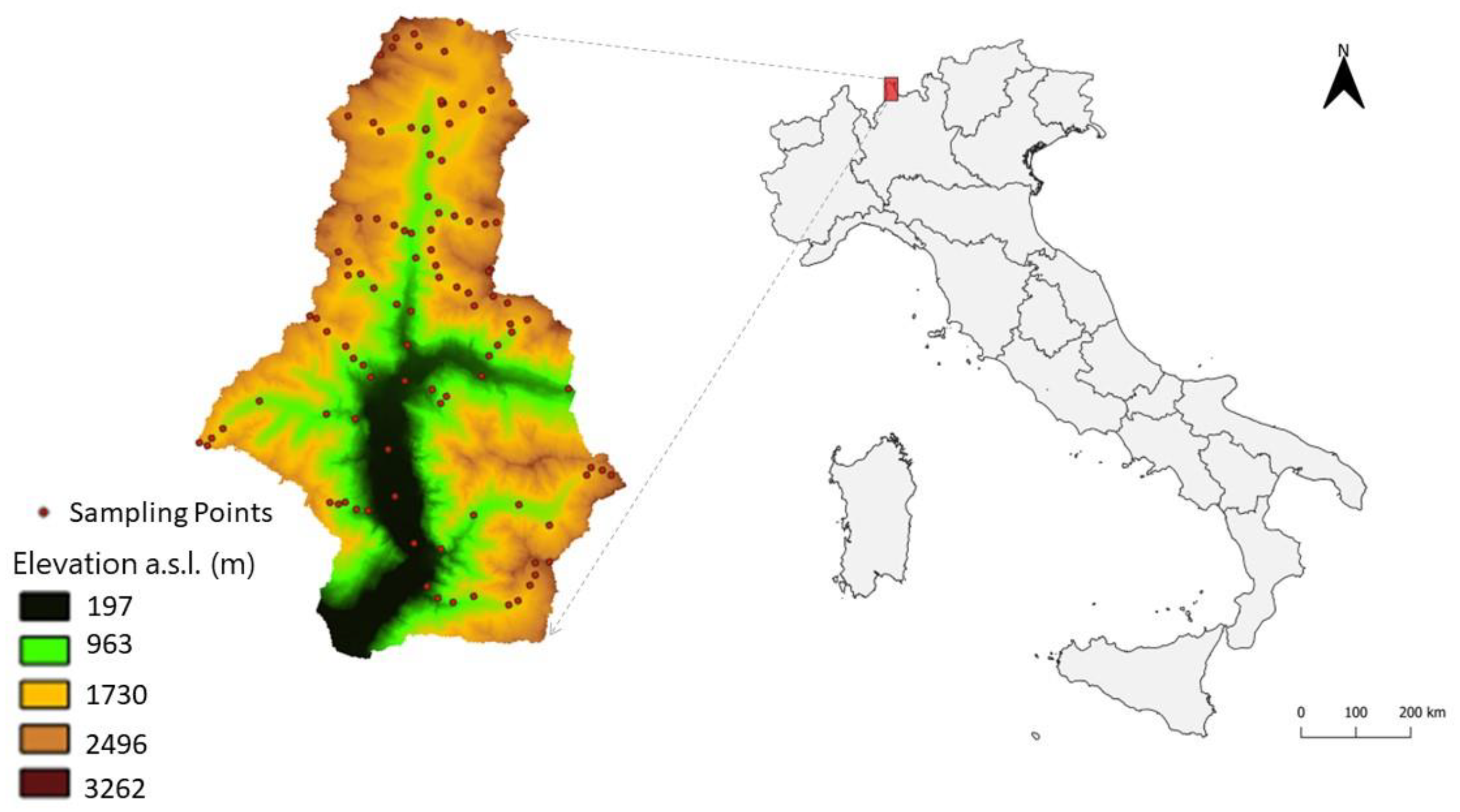

Table 1.
Main statistics of climate and geomorphometric covariates extracted from the 20 m DTM.
| Covariates Names | Abbreviations | Main statistics | ||||
|---|---|---|---|---|---|---|
| Min | Mean | Median | Max | SD | ||
| Elevation (m) | Elv | 197 | 1558.57 | 1664.21 | 3262 | 723.48 |
| Slope (°) | Slp | 0 | 31.75 | 32.93 | 80.08 | 15.40 |
| Northness index | N_ind | -0.99 | -0.14 | -0.31 | 1 | 0.74 |
| Eastness index | E_ind | -0.99 | -0.05 | -0.07 | 0.99 | 0.67 |
| Profile Curvature | Pr_cur | -0.277 | -0.000118 | -0.00003 | 0.208 | 0.007 |
| Plan Curvature | Pl_cur | -14.224 | 0.000095 | 0.00062 | 8.503 | 0.045 |
| Min Curvature | Min_cur | -0.666 | -0.010872 | -0.00515 | 0.242 | 0.023 |
| Log Curvature | Log_cur | -0.919 | -0.000248 | -0.00004 | 0.680102 | 0.039003 |
| General Curvature | Gen_cur | -1.426 | 0.000063 | 0 | 1.167034 | 0.07111 |
| Max Curvature | Max_cur | -0.309 | 0.010903 | 0.00539 | 0.483 | 0.022 |
| Transversal Curvature | Tra_cur | -0.773112 | 0.000311 | 0.00007 | 0.829 | 0.04 |
| Total Curvature | Tot_cur | 0 | 0.000986 | 0.00015 | 0.319 | 0.003 |
| Tang Curvature | Tan_cur | -0.269201 | 0.000099 | 0.000071 | 0.298031 | 0.014142 |
| Terrain Ruggedness Index | TRI | 0.0013 | 11.09 | 10.27 | 94.32 | 7.119 |
| Terrain Position Index | TPI | -81.178 | 0.0055 | -0.0012 | 65.2903 | 4.351 |
| Flow Accumulation | Fl_Acc | 0 | 106.35 | 3 | 61576 | 1109.12 |
| Vector Ruggedness Measure | VRM | 0 | 0.09 | 0.06 | 0.75 | 0.06 |
| Terrain Wetness Index | TWI | 2.808 | 7.944 | 7.324 | 19.311 | 2.715 |
| Mean annual Temperature (°C) | T | 1.62 | 4.97 | 3.12 | 14.61 | 3.74 |
| Mean annual Precipitations (mm) | P | 514.8 | 1278.56 | 1268.6 | 1531.1 | 132.39 |
Table 2.
Analytical data of Valchiavenna soils.
| Soil Properties | Statistical Metrics | ||||||
|---|---|---|---|---|---|---|---|
| Min | 1st Qu | Median | Mean | 3rd Qu | Max | SD | |
| SOC stock 10(kg.m-2) | 0.02 | 2.88 | 4.00 | 4.29 | 5.55 | 9.31 | 2.10 |
| SOC stock 30(kg.m-2) | 0.03 | 5.13 | 7.27 | 8.72 | 10.93 | 29.90 | 5.51 |
Table 3.
Validation performance of the different investigated machine learning models.
| Model Performance | Machine learning models | ||||
|---|---|---|---|---|---|
| MARS | Enet | RF | SVR | ||
| SOC stock 10(kg m-2) | RMSE | 1.63 | 1.61 | 1.35 | 1.50 |
| R2 | 0.39 | 0.41 | 0.69 | 0.50 | |
| MAE | 1.25 | 1.23 | 1.10 | 0.98 | |
| SOC stock 30(kg m-2) | RMSE | 3.47 | 3.97 | 3.36 | 3.46 |
| R2 | 0.45 | 0.48 | 0.65 | 0.62 | |
| MAE | 2.67 | 3.01 | 2.48 | 2.25 | |
Disclaimer/Publisher’s Note: The statements, opinions and data contained in all publications are solely those of the individual author(s) and contributor(s) and not of MDPI and/or the editor(s). MDPI and/or the editor(s) disclaim responsibility for any injury to people or property resulting from any ideas, methods, instructions or products referred to in the content. |
© 2023 by the authors. Licensee MDPI, Basel, Switzerland. This article is an open access article distributed under the terms and conditions of the Creative Commons Attribution (CC BY) license (http://creativecommons.org/licenses/by/4.0/).
Copyright: This open access article is published under a Creative Commons CC BY 4.0 license, which permit the free download, distribution, and reuse, provided that the author and preprint are cited in any reuse.


