
Submitted:
06 December 2023
Posted:
06 December 2023
You are already at the latest version
Abstract
The fluctuations in both time and space of the fish larvae community in relation to hydrographic characteristics in the waters surrounding the Taiwan Bank were studied in October 2021 (autumn) and March 2022 (spring). Throughout the study period, we identified a total of 149 taxa of fish larvae, encompassing 96 genera and 71 families. Engraulis japonicus, Diaphus slender type, unidentified Gobiidae, Apogon sp., unidentified Clupeidae, and Benthosema pterotum were the six most dominant taxa, together constituted 47.39% of the total catch. No significant temporal difference in abundance of fish larvae was found, but the species number of fish larvae was more diverse in spring than in autumn. There was a notable difference in species composition between the cruises, and the cluster analysis unveiled a distinct temporal structure in the assemblage of fish larvae. The dynamics of prevailing currents induced by seasonal monsoons play an important role in the transport of fish larvae. The distribution of fish larvae was closely linked to hydrographic features, where seawater temperature and salinity emerged as the primary explanatory factors influencing the composition of fish larvae assemblages in the waters surrounding the Taiwan Bank. While the increased influx of nutrients from upwelling ensures abundant food availability, the hydrographic conditions may not be suitable for every fish larva.
Keywords:
topographic upwelling
; currents
; seasonal monsoons
; larval dispersal
; Taiwan strait
1. Introduction
The composition of fish larvae assemblages arises from the convergent spawning strategies employed by various species, capitalizing on favorable environmental conditions to enhance larval survival [1,2]. In continental shelf waters characterized by tropical and subtropical climates, the distribution pattern of fish larvae assemblages is complex [3,4,5]. Due to the early ontogenetic stages of fish developing in the planktonic environment, they are influenced by both physical factors such as temperature, salinity, and currents, as well as biological factors like food availability and predator stocks [5,6]. The variability of these processes directly or indirectly impacts the distribution and survival of fish larvae, resulting in significant fluctuations in the annual recruitment of species [7]. Thus, the connection between fish larvae assemblages and physical-biological processes is gaining greater significance in the context of ecosystem-based fishery management and fishery-independent stock assessments [5,6].
The Taiwan Strait, sandwiched between mainland China and the island of Taiwan, is a shallow channel (~60 m) of 350 km in length and 180 km in width. It serves as a crucial link connecting the East China Sea (ECS) with the South China Sea (SCS), playing a significant role in the exchange of biota between these two seas. The Taiwan Strait experiences pronounced seasonal variations in currents, primarily influenced by the East Asian monsoon system and bathymetric topography [8,9]. In this region, there are three primary currents: (i) the cold, low saline, and nutrient-rich China Coastal Current (CCC), (ii) the warm and low saline South China Sea Warm Current (SCSC), and (iii) the warm, high saline, and oligotrophic Kuroshio Branch Current (KBC). During the cold season when the northeasterly monsoon is predominant, the CCC flows in a southward direction along the coast of mainland China and into the central Taiwan Strait. Simultaneously, the KBC courses through the Luzon Strait, extending into the northern SCS and the southeastern Taiwan Strait [8,10]. As the northeasterly monsoon weakens and transitions into the southwesterly monsoon in late spring, the SCSC gradually displaces the KBC, flowing in a northward direction into the northern Taiwan Strait [8,9].
The bathymetric topography in the Taiwan Strait is complex. It includes a shallow shelf along the Chinese coast, the Chang-Yuen Ridge, the Taiwan Bank, and the Penghu Channel [11]. Among these topographies, the Taiwan Bank, situated in the southern part of the Taiwan Strait, is characterized by sand dunes with the average water depth of ~20 m. The formation of an upwelling area may have different mechanisms. As reported by Tang et al. [12] and Hu et al. [13], multiple upwelling regions have been recognized in the Taiwan Strait, with one notable example being the Taiwan Bank Upwelling. The Taiwan Bank Upwelling (Figure 1), characterized by a banana-shaped area covering approximately 2500-3000 km2 and situated near the southern edge of the Taiwan Bank, occurs consistently throughout the year, primarily in the summer, exhibiting variable strengths and scales [12,13,14]. This upwelling region is the most important fishing ground in the Taiwan Strait for the stich-held dispnet, pole and line, longline fishing, and gill net fisheries.
While upwelling regions make up only 0.1% of the world ocean, their significance in fisheries production is noteworthy, contributing to nearly half of the world's total fisheries production [15,16]. Therefore, a good understanding on hydrographic and biological variations is essential for fish production and further resource management. Previous studies have distinctly highlighted the significance of coastal upwelling for the ecosystem of the Taiwan Strait, including its impact on the distribution pattern and succession of fish larvae assemblages [17,18]. However, our understanding on the fish larvae assemblage and on its response to environmental variables in the area of this study is lacking. The aims of the study were to: (i) compare the taxonomic compositions, abundances, and assemblages of fish larvae in the waters surrounding the Taiwan Bank between autumn and spring; and (ii) evaluate the effects of monsoon-driven currents and topographic upwelling on the distributional patterns of fish larvae assemblages.
2. Materials and Methods
2.1. Oceanographic and Biological Sampling
Two cruises of the R/V New Ocean Researcher 3 in the waters surrounding the Taiwan Bank was carried out during 19-21 October 2021 (hereafter autumn) and 8-11 March 2022 (hereafter spring) (Figure 2). Zooplankton samples were respectively collected at eight and ten stations in the autumn and spring cruises day and night using an Ocean Research Institute (ORI) net (6 m-long with a 1.6 m mouth diameter and a 330 μm mesh size). The net was towed vertically at a speed of approximately 1 m s-1, starting from a depth of 200 m (or 10 m above the bottom at stations with a depth of <210 m) up to the surface. The volume of filtered water was estimated by employing a flowmeter (Hydro-Bios, Kiel, Schleswig-Holstein, Germany) installed at the center of the net. The water volume filtered in each station ranged from 125 to 1036 m3. Upon retrieval from the ocean, the zooplankton samples were promptly preserved by immersion in a solution of 5% buffered formalin-seawater. At each station, before collecting zooplankton, vertical profiles (lowered from the surface to 10 m above the bottom) of temperature, salinity, and fluorescence were acquired using a General Oceanic SeaBird CTD (SEB-911 plus, Bellevue, Washington, USA).
2.2. Identification and Enumeration
In the laboratory, each zooplankton sample was divided into two subsamples with a Folsom plankton splitter (Aquatic Research Instruments, Wellington, New Zealand). Fish larvae were sorted from one randomly selected subsample and subsequently preserved in 95% alcohol after the sorting process. Fish larvae were identified to the lowest taxonomic level possible, relying on their morphological characteristics in accordance with Okiyama [19], Leis and Trnski [20], and Chiu [21]. The second subsample was successively divided until the number of individuals in the final subsample reached 1000-2000 or fewer. This subsample was then utilized to calculate the abundance of zooplankton. The abundances of fish larvae and zooplankton were quantified as the number of individuals per 1000 m3 and 1 m3, respectively.
2.3. Statistical Analyses
Vertical profiles of temperature and salinity at the upper 50 m were diagramed using SURFER 8.01 software (Golden Software, Inc., Golden, Colorado, USA). The Shannon-Wiener diversity index (H′) [22] and Pielou’s index of evenness (J′) [23] were computed to assess the temporal variations in species diversity and the relative abundances of species in a community, respectively. Non-parametric Mann-Whitney U-test [24] was used to determine the significance of differences between cruises in hydrographic variables and abundance and diversity of fish larvae. To examine temporal and spatial variations in the fish larvae assemblage, we utilized the multivariate statistical software PRIMER version 6 (PRIMER-E, West Hoe, Plymouth, UK). Before conducting the analysis, data on fish larvae abundance (those constituting >1% of the total larvae catch) were log(x+1)-transformed to mitigate the influence of dominant taxa, following the approach outlined by Clarke and Warwick [25]. A triangular similarity matrix between sampling stations, used to generate a cluster dendrogram, was built using Bray-Curtis similarities [26]. Meanwhile, non-metric multi-dimensional scaling (MDS) [27] was applied to provide a two-dimensional visual representation of the assemblage structure. The similarity percentage routine (SIMPER) [28] was employed to illustrate the percentage contribution of each taxon to the average similarities within the different fish larvae assemblages. Furthermore, the distance-based linear models (DistLM, one program of the multivariate statistical software of PERMANOVA+ for PRIMER) [29] was chosen to evaluate the relationship between hydrographic variables and fish larvae assemblages. These models were constructed using the stepwise selection procedure with the adjusted R2 serving as the selection criterion. Ultimately, the full model was visualized by inspecting the distance-based redundancy analysis (dbRDA) [30] ordination.
3. Resaults
3.1. Hydrographic and Biological Conditions
The surface seawater at 10-m depth in the waters surrounding Taiwan Bank showed clear temporal change in temperature (Mann-Whitney U-test, U = 0, P < 0.001). Higher mean value of temperature was observed in autumn than in spring (Table 1). In autumn the temperature ranged from 26.86°C to 28.94°C, compared to spring when it ranged from 20.11°C to 24.80°C. Analysis of vertical profiles of temperature showed that the water column was well mixed vertically in both cruises (Figure 3). Examining the whole study area, the distribution pattern of isotherms displayed a northwest-southeast gradient, and the temperatures increased gradually from high to low latitudes, particularly in spring (20 to 25°C).
Surface seawater salinity fluctuated from 33.91 to 34.05 in autumn and from 33.79 to 34.33 in spring. The distinct difference of surface salinity between cruises was observed (Table 1), with significantly higher salinity recorded in spring than in autumn (Mann-Whitney U-test, U = 8, P < 0.01). Salinity were generally lower in the southern Taiwan Bank in autumn, such as stations B7, B32, and B33; on the contrary, slightly lower salinities were recorded in the northern Taiwan Bank in spring, but no significant spatial difference was observed (Figure 3).
Fluorescence showed no significant temporal difference (Mann-Whitney U-test, U = 37, P = 0.790). In the study, fluorescence ranged from 0.08 mg m-3 to 1.40 mg m-3 in autumn and from 0.06 mg m-3 to 1.86 mg m-3 in spring. Slightly higher mean value was recorded in spring (Table 1). In general, higher values (>1.00 mg m-3) were found on the northern side of the bank (within or adjacent to upwelling area), with the highest values found at station B10 and B6 for both cruises, respectively (Figure 4).
Zooplankton abundance varied from 108 ind. m-3 to 791 ind. m-3 in autumn and from 175 ind. m-3 to 832 ind. m-3 in spring, with the mean of 381 ± 227 (SD) ind. m-3 and 451 ± 226 ind. m-3, respectively. No significant difference in zooplankton abundance was observed between cruises (Mann-Whitney U-test, U = 31, P = 0.424). The distribution pattern of zooplankton abundance showed significant positive correlation with fluorescence (Simple regression analysis, F = 5.948, P < 0.05), also usually having a higher abundance at stations B6, B10, and B14 (Figure 4).
3.2. Composition of Fish Larvae
A total of 1968 fish larvae specimens were collected by the present study, in which 149 taxa or morphotypes were identified belonging to 71 families and 96 genera. Among these specimens, a large number of individuals were unidentified (which constituted 2.91% of the total catch) and yolk-sac larvae (which constituted 6.01% of the total catch), while others were specimens damaged during collection (which constituted 0.99% of the total catch). Larvae of the families Myctophidae, Engraulidae, Gobiidae, Apogonidae, Clupeidae, and Bregmacerotidae were the most abundant in the study and accounted for 23, 13, 10, 7, 6, and 5% of the total catch, respectively. Among them, Myctophidae had the largest number of species (19 taxa), followed by Gobiidae (6 taxa), Bregmacerotidae (3 taxa), Engraulidae (2 taxa), Apogonidae (2 taxa), and Clupeidae (1 taxon). The most frequent captured families (>1% of the total fish larvae) in both cruises are ranked in Table 2. The top five dominant families in autumn were Engraulidae, Gobiidae, Apogonidae, Bregmacerotidae, and Myctophidae; by contrast, the predominant families in spring were Myctophidae, Clupeidae, Ammodytidae, Gobiidae, and Sparidae.
At the species level, Engraulis japonicus constituted 12.71% of the total catch, representing the most abundant taxon during the survey. Diaphus slender type (12.71%), unidentified Gobiidae (7.57%), Apogon sp. (6.77%), unidentified Clupeidae (6.26%), and Benthosema pterotum (5.11%) were the next five most abundant fish larvae. These six taxa together constituted 47.39% of the total larval abundance. During the two cruises the species compositions of dominant fish larvae differed significantly (Table 3). In autumn, E. japonicus, Apogon sp., unidentified Gobiidae, Bregmaceros sp., unidentified Myctophidae, Tridentiger sp., and Trichiurus lepturus were abundant, accounting for 65.65% of total fish larvae numerical abundance. Among these seven taxa, the abundance of E. japonicus was significantly higher than that of the other taxa, with a peak abundance of 877 ind. 1000 m-3 at station B10. In spring, the five most dominant taxa were Diaphus slender type, unidentified Clupeidae, B. pterotum, Bleekeria mitsukurii, and unidentified Gobiidae, contributing 51.89% to spring total catch. The three dominant taxa, namely Diaphus slender type, unidentified Clupeidae, and B. pterotum, showed significantly higher abundance at stations B17 (521 ind. 1000 m-3), B14 (442 ind. 1000 m-3), and B6 (163 ind. 1000 m-3), respectively.
3.3. Temporal Changes in Abundance and Diversity of Fish Larvae
The overall mean abundance (mean ± SD) during the study period was 415 ± 358 ind. 1000 m-3, ranging from 97 ind. 1000 m-3 to 1227 ind. 1000 m-3 in autumn and 29 ind. 1000 m-3 to 1025 ind. 1000 m-3 in spring, respectively. The mean abundance was slightly higher in autumn than in spring (Table 1), but no significant temporal difference was found in abundance of fish larvae (Mann-Whitney U-test, U = 30, P = 0.374). No distinct distribution difference of abundance was observed for both cruises (Figure 5). Nevertheless, relatively higher abundances of fish larvae occurred at stations B10, B11, and B15 in autumn and at stations B6, B7, B14, and B17 in spring, respectively.
No significant temporal difference was found in the species number of fish larvae (Mann-Whitney U-test, U = 31, P = 0.422), although the total number of fish larvae species occurred in spring was greater than in autumn (Table 1). Fish larvae in 37 families, 46 genera, and 66 taxa were identified in autumn. Autumn species diversity and species evenness of fish larvae varied among stations, from 0.86 to 2.78 and from 0.44 to 0.89, respectively. In contrast to autumn, 104 taxa belonging to 51 families and 61 genera were recorded in spring, with species diversity and species evenness fluctuated from 0.45 to 2.91 and from 0.55 to 0.93, respectively. Species diversity (Mann-Whitney U-test, U = 34, P = 0.594) and species evenness (Mann-Whitney U-test, U = 37, P = 0.789) also showed no significant temporal differences (Table 1). Overall, the distributions of the diversity and evenness were consistent with the pattern of species number.
3.4. Assemblages of Fish Larvae
The dendrogram from the cluster analysis of Bray-Curtis similarity matrices based on 18 fish larvae taxa (each with a relative abundance >1%) defined three station groups at a similarity level of 16% (Figure 6). A clear structure corresponding with the sampling seasons was observed for the assemblages of fish larvae. The percentage contributions of the dominant taxa in each station group are shown in Table 4.
Group A consisted of only one station (station B10 in spring), and had the lowest species number and species diversity (0.45) among all the sampling stations. Two fish larvae taxa (unidentified Mullidae and Upeneus japonicus), both belonging to coastal and benthic species, were found in this group.
Group B (autumn assemblage) included all autumn stations. The dominant fish larvae taxa in this station group were Engraulis japonicus, Apogon sp., unidentified Gobiidae, Bregmaceros sp., unidentified Myctophidae, Tridentiger sp., and Trichiurus lepturus. The SIMPER routine identified unidentified Gobiidae and unidentified Myctophidae were the most important discriminators (Sim/SD >1) for this group (Table 4). In addition, two commercial species, E. japonicus and T. lepturus, were prevalent in this station group, providing the contribution of 6.46% and 6.33% to this group, respectively.
Group C (spring assemblage) was comprised of nine spring stations. Diaphus slender type, unidentified Clupeidae, Benthosema pterotum, Bleekeria mitsukurii, and unidentified Gobiidae were the dominant taxa in this station group. Among them, Diaphus slender type showed the highest abundance of 521 ind. 1000 m-3, at station B17 adjacent to southwestern Taiwan. While, unidentified Clupeidae, B. pterotum, B. mitsukurii showed the highest abundance at station B14 with values of 442, 80, and 116 ind. 1000 m-3, respectively. The SIMPER routine identified mesopelagic species B. pterotum was the most important discriminator (Sim/SD >1) for this group, with a contribution of 36.77% (Table 4). In addition, two commercial (Trichiurus lepturus and Planiliza sp.) and two coastal (Cubiceps pauciradiatus and B. mitsukurii) were also important in this group, with a combined percentage contribution of 54.98%.
3.5. Correlation between Fish Larvae Assemblages and Environmental Variables
The distance-based linear model was used to examine the relationship between fish larvae assemblages and environmental variables. All five environmental variables together explained 54.56% of the total variation (Table 5). Seawater temperature (26.76%, P = 0.001) and salinity (13.10%, P = 0.026) were the only two significant explanatory variables to affect the assemblage structure of fish larvae in the waters surrounding the Taiwan Bank. For the fitted model, the dbRDA biplot showed axes 1 and 2 explained 58.1% and 22.5% of the variance, which corresponded to 31.6% and 12.3% of the total variance in the original Bray-Curtis similarity matrix (Figure 7). The change in assemblages of fish larvae between cruises corresponded with decreasing seawater temperature and increasing salinity.
4. Discussion
The spatiotemporal variations in water masses surrounding the Taiwan Bank and their through-flow transports are influenced by the seasonal monsoon system and bathymetric topography [8,10]. The waters surrounding the Taiwan Bank, dominated by the CCC, SCSC, and KBC, belong to the tropical western North Pacific. During winter, the northeasterly monsoon pushes the warm and hyper-saline KBC northward through the Penghu Channel into the southeastern Taiwan Strait, while the cold and less salty CCC moves southward along the western boundary of the Strait. When the northeasterly monsoon subsides in late spring, the warm and low-salinity SCSC flows northeastward, synchronizing with the southwesterly monsoon, intruding into the Taiwan Strait and dominating this region [8,9,10]. In the present study, the surface seawater temperature throughout the study area was >26.5°C in autumn and between 20~25°C in spring. In both cruises, the distribution of isotherms exhibited a northwest-to-southeast gradient, with temperatures gradually rising from higher to lower latitudes (Figure 3). On the contrary, the surface salinity distribution demonstrated a contrasting pattern between the cruises. In autumn, slightly lower salinity values were observed in the southern Taiwan Bank, while in spring, these lower values were found in the northern Taiwan Bank. The findings highlighted the influence of the currents mentioned earlier on the hydrographic conditions surrounding the Taiwan Bank during our study period. Specifically, the SCSC played a significant role in autumn, while the CCC and KBC were prominent factors in spring.
Upwelling is not just a hydrographic phenomenon; it also has a significant impact on marine ecosystems. The upwelling phenomenon on the Taiwan Bank is caused by the combined influence of two factors: bathymetric topography and northward currents [17]. The rising bottom water in this study area provided an additional influx of nutrient-rich water, in turn, enhanced the nutrients and phytoplankton, leading to an increase in the abundance of zooplankton [31,32,33]. In the present study, outstandingly high fluorescence values, indicating a high phytoplankton biomass, were observed at stations situated within or near the upwelling area. Furthermore, our findings revealed a close relationship between the distribution pattern of zooplankton abundance and fluorescence (Figure 4). In marine pelagic ecosystems, the population growth of zooplankton is typically associated with high phytoplankton biomass [32,33]. In the absence of river discharges, we believed that the elevated fluorescence and zooplankton abundance observed at the above-mentioned stations were likely a result of nutrients being upwelled to the surface through topographic upwelling. Furthermore, during winter and early spring, the northeasterly monsoon disrupts the summer thermal stratification, enabling upwelling to transport more nutrients into the mixed layer. This inference could be substantiated by the observation that fluorescence and zooplankton abundance in spring were slightly higher than in autumn throughout the study period. Similarly, elevated chlorophyll a concentration was documented in the Taiwan Bank Upwelling, as reported by studies conducted by Huang et al. [34] and Hsiao et al. [14].
Upwelling areas are often regarded as good fishing grounds because of the elevated primary productivity linked to the nutrients brought up by the upwelling process [14,15]. Surface convergence resulting from upwelling can lead to the accumulation of diverse fish larvae assemblages [4,35]. The present study detected two major fish larvae assemblages, comprising 149 taxa from 71 identifiable families, corresponding closely with the sampling seasons (Figure 6). The existence of such diverse fish larvae further reflects the fact that the waters surrounding the Taiwan Bank are considered a major transition zone between tropical and subtropical faunas. The influx of larvae and early juveniles from numerous tropical-oceanic species into subtropical-neritic waters through the Taiwan Strait enhances these assemblages [36,37].
Spatiotemporal variations in the taxonomic composition of assemblages and in the abundance of individual taxon of fish larvae were evident in the waters surrounding the Taiwan Bank. In this study, the two primary seasonal assemblages of fish larvae were distinct from one another in terms of both the variety of species and the number of individual larvae present. This distinct difference can be attributed to the prevalence of neritic/oceanic-epipelagic species in the autumn assemblage and neritic/mesopelagic species in the spring assemblage. Analyzing the prevalent fish larvae compositions during two cruises, aside from the presence of demersal taxa overlap, such as unidentified Gobiidae, the autumn assemblage was defined by Engraulis japonicus, Apogon sp., and Bregmaceros sp. On the other hand, the spring assemblage was primarily led by lanternfishes like Diaphus slender type and Benthosema pterotum, unidentified Clupeidae, and Bleekeria mitsukurii (Table 3). We speculated two potential sources for the presence of these fish larvae in the waters surrounding the Taiwan Bank: (i) the spawning and hatching of subtropical coastal fish within the study area; and (ii) the origin of oceanic mesopelagic fish larvae from the KBC or the SCSC.
Here we substantiate the above speculations with two examples. Engraulis japonicus is among the most plentiful and commercially small pelagic fish, commonly occurring in subtropical to temperate waters of the Indo-Pacific. The harvesting of larval anchovy is a significant economic activity in the coastal regions of Taiwan [38,39]. In the western North Pacific, coastal populations of E. japonicus are distributed along the continental coast from Korea to southeastern China. According to Lee et al. [38] and Tu et al. [40], adults of E. japonicus migrate from the East China Sea to the coastal waters of Taiwan primarily during winter and spring for spawning. Nevertheless, the appearance of E. japonicus in autumn is surprising since the predominant currents in the Taiwan Strait typically move in a northerly direction [41]. Remarkably, a comparable increase in E. japonicus larvae during autumn was also noted in the I-lan Bay of northeast Taiwan [42]. A potential explanation is that the adults of E. japonicus might swim southward to reach their spawning grounds along the coast of Mainland China, where the northerly flow is notably weak and not persistent in autumn [41].
Mesopelagic fish larvae primarily dwell in the deeper oceanic waters [43]. Their larvae are especially abundant in the Kuroshio Current and offshore oceanic waters [44,45]. Sassa et al. [44,46] reported that in the waters of the Kuroshio axis off Japan and the offshore side of the Kuroshio axis off southern Japan, mesopelagic fish larvae typically accounted for more than 85% of the total fish larvae catch. Hence, these mesopelagic fish larvae served as reliable indicators for the intrusion of the KBC into the Taiwan Strait. We proposed that these species were carried into the waters of the Taiwan Bank by the KBC. This conclusion finds support in the greater species number and abundance of mesopelagic fish larvae observed in spring (Table 2), indicating the accumulation of these taxa during this specific period. Similarly, Lee et al. [47] and Hsieh et al. [36,37] suggested that the intrusion of the KBC could potentially carry myctophid larvae from the Kuroshio region to the Taiwan Strait and the coastal waters off southwestern Taiwan, as supported by their respective studies. Yet, the simultaneous presence of mesopelagic fish larvae alongside larvae of coastal epipelagic and demersal species, such as anchovies and gobiid fishes, likely suggests the potential for interspecific competition among these different species. This is because mesopelagic fish larvae have been identified as potential competitors for the prey of commercially important fish larvae in oceanic regions, as indicated by studies such as Ahlstrom [48] and Sabatés and Masó [49].
Past studies have confirmed the crucial role of food availability in determining the distribution and survival of fish larvae, especially at the very early life stages when the yolk is depleted [2,5]. The plankton aggregation and production enhancement in the upwelling area could provide favorable feeding conditions for fish larvae. However, physical factors such as seawater temperature and salinity also play a significant role in determining the survival of fish larvae during their early life stages and influencing the success of population recruitment [2,5,50]. In this study, the findings from the distance-based linear model showed a clear distributional pattern of fish larvae assemblage associated with seawater temperature and salinity (Table 5, Figure 7). During spring, specific mesopelagic fish larvae, including Diaphus slender type, Ceratoscopelus warmingii, and Myctophum asperum, were predominantly found on the southern side of the bank (such as stations B7 and B17), where salinity levels were relatively higher. In contrast, these taxa were not present on the northern side of the bank (for example, stations B5, B10, and B14). Additionally, the distribution pattern of spring fish larvae exhibited a positive correlation with salinity. Considering the habitat of adult mesopelagic fishes, their larvae in the North Pacific are typically found in waters with high salinity levels [46,51]. We speculated that while the intrusions of the KBC or SCSC transported mesopelagic fish larvae into the waters surrounding the Taiwan Bank, the relatively lower salinity waters on the northern side of the bank during spring might be unsuitable for mesopelagic fish larvae. This unfavorable environment could potentially lead to low larval survival despite the abundant food availability in this area.
5. Conclusions
In conclusion, this study demonstrated that the temporal change of fish larvae abundance between autumn and spring was not significant, but fish larvae were more diverse in spring than in autumn. The transport of fish larvae is notably affected by the fluctuating currents generated by seasonal monsoons. Despite the enriched food supply resulting from additional nutrient influx through upwelling, the hydrographic conditions may not be favorable for every fish larva. Besides, the strong correlation observed between hydrographic variables (specifically seawater temperature and salinity) and fish larvae assemblages further suggests the possible use of these assemblages as tracers for surface circulation in the waters surrounding Taiwan Bank. The present study not only enhances our understanding of ecosystems in the region but also serves as good examples of biotic responses to the hydrographic conditions and interactions among water masses.
Author Contributions
For research articles with several authors, a short paragraph specifying their individual contributions must be provided. The following statements should be used “Conceptualization, H.-Y.H. and M.-A.L.; methodology, H.-Y.H. and P.-J.M.; software, H.-Y.H. and W.-L.C.; formal analysis, W.-L.C.; investigation, H.-Y.H. and W.-L.C.; resources, H.-Y.H. and P.-J.M.; writing—original draft preparation, H.-Y.H.; writing—review and editing, H.-Y.H. and P.-J.M.; supervision, H.-Y.H.; project administration, H.-Y.H. and M.-A.L.; funding acquisition, H.-Y.H. All authors have read and agreed to the published version of the manuscript.
Funding
This research was funded by the National Science Council and the Ministry of Education of the Republic of China to H.-Y. Hsieh (MOST 110-2611-M-259-001).
Institutional Review Board Statement
Not applicable.
Informed Consent Statement
Any research article describing a study involving humans should contain this statement. Please add “Informed consent was obtained from all subjects involved in the study.” OR “Patient consent was waived due to REASON (please provide a detailed justification).” OR “Not applicable.” for studies not involving humans. You might also choose to exclude this statement if the study did not involve humans. Written informed consent for publication must be obtained from participating patients who can be identified (including by the patients themselves). Please state “Written informed consent has been obtained from the patient(s) to publish this paper” if applicable.
Data Availability Statement
We encourage all authors of articles published in MDPI journals to share their research data. In this section, please provide details regarding where data supporting reported results can be found, including links to publicly archived datasets analyzed or generated during the study. Where no new data were created, or where data is unavailable due to privacy or ethical restrictions, a statement is still required. Suggested Data Availability Statements are available in section “MDPI Research Data Policies” at https://www.mdpi.com/ethics.
Acknowledgments
We express our gratitude to the captain, officers, and crew of the R/V New Ocean Researcher 3 for their skillful assistance in collecting zooplankton samples and other hydrographic data.
Conflicts of Interest
The authors declare no conflict of interest.
References
- Franco-Gordo, C.; Godínez-Domínguez, E.; Suárez-Morales, E. Larval fish assemblages in waters off the central Pacific coast of Mexico. J. Plankton Res. 2002, 24, 775–784. [Google Scholar] [CrossRef]
- Sabatés, A.; Olivar, M.P.; Salat, J.; Palomera, I.; Alemany, F. Physical and biological processes controlling the distribution of fish larvae in the NW Mediterranean. Prog. Oceanogr. 2007, 74, 355–376. [Google Scholar] [CrossRef]
- Young, P.C.; Leis, J.M.; Hausfeld, H.F. Seasonal and spatial distribution of fish larvae in waters over the North West Continental Shelf of Western Australia. Mar. Ecol. Prog. Ser. 1986, 31, 209–222. [Google Scholar] [CrossRef]
- Doyle, M.J.; Morse, W.W.; Kendall, A.W.J. A comparison of larval fish assemblages in the temperate zone of the northeast Pacific and northwest Atlantic Oceans. Bull. Mar. Sci. 1993, 53, 588–644. [Google Scholar]
- Olivar, M.P.; Emelianov, M.; Villate, F.; Uriarte, I.; Maynou, F.; Álvarez, I.; Morote, E. The role of oceanographic conditions and plankton availability in larval fish assemblages off the Catalan coast (NW Mediterranean). Fish. Oceanogr. 2010, 19, 209–229. [Google Scholar] [CrossRef]
- Bakun, A. Fronts and eddies as key structures in the habitat of marine fish larvae: opportunity, adaptive response and competitive advantage. Sci. Mar. 2006, 70, 105–122. [Google Scholar] [CrossRef]
- Govoni, J.J. Fisheries oceanography and the ecology of early life histories of fishes: a perspective over fifty years. Sci. Mar. 2005, 69, 125–137. [Google Scholar] [CrossRef]
- Jan, S.; Wang, J.; Chern, C.S.; Chao, S.Y. Seasonal variation of the circulation in the Taiwan Strait. J. Mar. Syst. 2002, 35, 249–268. [Google Scholar] [CrossRef]
- Jan, S.; Sheu, D.D.; Kuo, H.M. Water mass and throughflow transport variability in the Taiwan Strait. J. Geophys. Res. 2006, 111, C12012. [Google Scholar] [CrossRef]
- Wang, J.; Chern, C.S. On the Kuroshio branch in the Taiwan Strait during wintertime. Prog. Oceanogr. 1988, 21, 469–491. [Google Scholar]
- Chang, Y.; Shimada, T.; Lee, M.A.; Sakaida, F.; Kawamura, H. Wintertime sea surface temperature fronts in the Taiwan Strait. Geophys. Res. Lett. 2006, 33, L23603. [Google Scholar] [CrossRef]
- Tang, D.L.; Kester, D.R.; Ni, I.H.; Kawamura, H.; Hong, H.S. Upwelling in the Taiwan Strait during the summer monsoon detected by satellite and shipboard measurements. Remote Sens. Environ. 2002, 83, 457–471. [Google Scholar] [CrossRef]
- Hu, J.; Kawamura, H.; Hong, H.; Pan, W. A review of research on the upwelling in the Taiwan Strait. Bull. Mar. Sci. 2003, 73, 605–628. [Google Scholar]
- Hsiao, P.Y.; Shimada, T.; Lan, K.W.; Lee, M.A.; Liao, C.H. Assessing summertime primary production required in changed marine environments in upwelling ecosystem around the Taiwan Bank. Remote Sens. 2021, 13, 765. [Google Scholar] [CrossRef]
- Ryther, J.H. Photosynthesis and fish production in the sea. Science 1969, 166, 72–76. [Google Scholar] [CrossRef] [PubMed]
- Zhen, Z. Introduction. In Minnan-Taiwan Bank fishing ground upwelling ecosystem study (pp. i-ii); Hong, H.S., Qiu, S.Y., Ruan, W.Q., Hong, Q.C., Eds.; Science Publishing House: Beijing, China, 1991; pp. i–ii. (in Chinese) [Google Scholar]
- Hong, H.S.; Qiu, S.Y.; Ruan, W.Q.; Hong, Q.C. 1991. Minnan-Taiwan Bank fishing ground upwelling ecosystem study. In Minnan-Taiwan Bank fishing ground upwelling ecosystem study; Hong, H.S., Qiu, S.Y., Ruan, W.Q., Hong, Q.C., Eds.; Science Publishing House: Beijing, China, 1991; pp. 1–18. (in Chinese) [Google Scholar]
- Hsieh, H.Y.; Lo, W.T.; Wu, L.J.; Liu, D.C. Larval fish assemblages in the Taiwan Strait, western North Pacific: linking with monsoon-driven mesoscale current system. Fish. Oceanogr. 2012, 21, 125–147. [Google Scholar] [CrossRef]
- Okiyama, M. (Ed.) An Atlas of the Early Stage Fishes in Japan; Tokai University Press: Tokyo, Japan, 1988. (In Japanese) [Google Scholar]
- Leis, J.M.; Trnski, T. The Larvae of Indo-Pacific Shorefishes; New South Wales University Press: Sidney, Australia, 1989. [Google Scholar]
- Chiu, T.S. Fish larvae of Taiwan; National Museum of Marine Biology and Aquarium: Checheng, Taiwan, ROC, 1999. [Google Scholar]
- Shannon, C.E.; Weaver, W. The Mathematical Theory of Communication; University of Illinois Press: Urbana, IL, USA, 1949. [Google Scholar]
- Pielou, E.C. The measurement of diversity in different types of biological collections. J. Theor. Biol. 1966, 13, 131–144. [Google Scholar] [CrossRef]
- Mann, H.B.; Whitney, D.R. On a test of whether one of two random variables is stochastically larger than the other. Ann. Math. Stat. 1947, 18, 50–60. [Google Scholar] [CrossRef]
- Clarke, K.R.; Warwick, R.M. Change in Marine Communities: An Approach to Statistical Analysis and Interpretation, 2nd ed.; PRIMER-E: Plymouth, UK, 2001; 172p. [Google Scholar]
- Bray, J.R.; Curtis, J.T. An ordination of the upland forest communities of southern Wisconsin. Ecol. Monogr. 1957, 27, 325–349. [Google Scholar] [CrossRef]
- Kruskal, J.B.; Wish, M. Multidimensional Scaling; Sage University Paper Series on Quantitative Application in the Social Sciences; Sage Publications: Beverly Hills, CA, USA, 1978. [Google Scholar]
- Clarke, K.R. Non-parametric multivariate analyses of changes in community structure. Aust. J. Ecol. 1993, 18, 117–143. [Google Scholar] [CrossRef]
- Anderson, M.J. A new method for non-parametric multivariate analysis of variance. Aust. Ecol. 2001, 26, 32–46. [Google Scholar]
- McArdle, B.H.; Anderson, M.J. Fitting multivariate models to community data: a common on distance-based redundancy analysis. Ecology 2001, 82, 290–297. [Google Scholar] [CrossRef]
- Chung, S.W.; Jan, S.; Liu, K.K. Nutrient fluxes through the Taiwan Strait in spring and summer 1999. J. Oceanogr. 2001, 57, 47–53. [Google Scholar] [CrossRef]
- García-Comas, C.; Stemmann, L.; Ibanez, F.; Berline, L.; Mazzocchi, M.G.; Gasparini, S.; Picheral, M.; Gorsky, G. Zooplankton long-term changes in the NW Mediterranean Sea: Decadal periodicity forced by winter hydrographic conditions related to large-scale atmospheric changes? J. Mar. Syst. 2011, 87, 216–226. [Google Scholar] [CrossRef]
- Tommasi, D.; Hunt, B.P.V.; Pakhomov, E.A.; Mackas, D.L. Mesozooplankton community seasonal succession and its drivers: Insights from a British Columbia, Canada, fjord. J. Mar. Syst. 2013, 115–116, 10–32. [Google Scholar] [CrossRef]
- Huang, T.H.; Chen, C.T.A.; Bai, Y.; He, X. Elevated primary productivity triggered by mixing in the quasi-cul-de-sac Taiwan Strait during the NE monsoon. Sci. Rep. 2020, 10, 7846. [Google Scholar] [CrossRef]
- Gray, C.A.; Miskiewicz, A.G. Larval fish assemblages in south-east Australian coastal waters: seasonal and spatial structure. Est. Coast. Shelf Sci. 2000, 50, 549–570. [Google Scholar] [CrossRef]
- Hsieh, H.Y.; Meng, P.J.; Chang, Y.C.; Lo, W.T. Temporal and spatial occurrence of mesopelagic fish larvae during epipelagic drift associated with hydrographic features in the Gaoping coastal waters off southwestern Taiwan. Mar. Coast. Fish. 2017, 9, 244–259. [Google Scholar] [CrossRef]
- Hsieh, H.Y.; Lo, W.T.; Liao, C.C.; Meng, P.J. Shifts in the assemblage of summer mesopelagic fish larvae in the Gaoping waters of southwestern Taiwan: a comparison between El Niño events and regular years. J. Mar. Sci. Eng. 2021, 9, 1065. [Google Scholar] [CrossRef]
- Lee, M.A.; Lee, K.T.; Shiah, G.Y. Environmental factors associated with the formation of larval anchovy fishing grounds in the coastal waters of southwest Taiwan. Mar. Biol. 1995, 121, 621–625. [Google Scholar] [CrossRef]
- Chiu, T.S.; Young, S.S.; Chen, C.S. Monthly variation of larval anchovy fishery in I-lan Bay, NE Taiwan, with an evaluation for optimal fishing season. J. Fish. Soc. Taiwan 1997, 24, 273–282. [Google Scholar]
- Tu, C.Y.; Tseng, Y.H.; Chiu, T.S.; Shen, M.L.; Hsieh, C.H. Using coupled fish behavior-hydrodynamic model to investigate spawning migration of Japanese anchovy, Engraulis japonicus, from the East China Sea to Taiwan. Fish. Oceanogr. 2012, 21, 255–268. [Google Scholar] [CrossRef]
- Lee, H.J.; Chao, S.Y. A climatological description of circulation in and around the East China Sea. Deep-Sea Res. Part II 2003, 50, 1065–1084. [Google Scholar] [CrossRef]
- Chiu, T.S.; Chen, C.S. Growth and temporal variation of two Japanese anchovy cohorts during their recruitment to the East China Sea. Fish. Res. 2001, 53, 1–15. [Google Scholar] [CrossRef]
- Nakabo, T. (Ed.) Fishes of Japan with Pictorial Keys to the Species, English ed.; Tokai University Press: Tokyo, Japan, 2002. [Google Scholar]
- Sassa, C.; Moser, H.G.; Kawaguchi, K. Horizontal and vertical distribution patterns of larval myctophid fishes in the Kuroshio Current region. Fish. Res. 2002, 11, 1–10. [Google Scholar] [CrossRef]
- Okazaki, Y.; Nakata, H. Effect of the mesoscale hydrographic features on larval fish distribution across the shelf break of East China Sea. Cont. Shelf Res. 2007, 27, 1616–1628. [Google Scholar] [CrossRef]
- Sassa, C.; Kawaguchi, K.; Hirota, Y.; Ishida, M. Distribution patterns of larval myctophid fish assemblages in the subtropical-tropical waters of the western North Pacific. Fish. Oceanogr. 2004, 13, 267–282. [Google Scholar] [CrossRef]
- Lee, M.A.; Wang, Y.C.; Chen, Y.K.; Chen, W.Y.; Wu, L.J.; Liu, D.C.; Wu, J.L.; Teng, S.Y. Summer assemblages of ichthyoplankton in the waters of the East China Sea shelf and around Taiwan in 2007. J. Mar. Sci. Technol. 2013, 21, 41–51. [Google Scholar]
- Ahlstrom, E.H. Mesopelagic and bathypelagic fishes in the California current region. Calif. Coop. Ocean. Fish. Invest. Rep. 1969, 13, 39–44. [Google Scholar]
- Sabatés, A.; Masó, M. Effect of a shelf-slope front on the spatial distribution of mesopelagic fish larvae in the Western Mediterranean. Deep-Sea Res. 1990, 37, 1085–1098. [Google Scholar] [CrossRef]
- Muhling, B.A.; Beckley, L.E.; Olivar, M.P. Ichthyoplankton assemblage structure in two mesoscale Leeuwin Current eddies, eastern Indian Ocean. Deep-Sea Res. Part II 2007, 54, 1113–1128. [Google Scholar] [CrossRef]
- Moser, H.G.; Smith, P.E. Larval fish assemblages and oceanic boundaries. Bull. Mar. Sci. 1993, 53, 283–289. [Google Scholar]
Figure 1.
SeaWiFS image on 2 August 1998 showing high chlorophyll concentrations in upwelling areas of Pingtan Upwelling (PTU), Meizhou-Xiaman Upwelling (MXU), Dongshan Upwelling (DSU), Taiwan Bank Upwelling (TBU), and Penhu Upwelling (PHU). Cited from Tang et al. (2002).
Figure 1.
SeaWiFS image on 2 August 1998 showing high chlorophyll concentrations in upwelling areas of Pingtan Upwelling (PTU), Meizhou-Xiaman Upwelling (MXU), Dongshan Upwelling (DSU), Taiwan Bank Upwelling (TBU), and Penhu Upwelling (PHU). Cited from Tang et al. (2002).
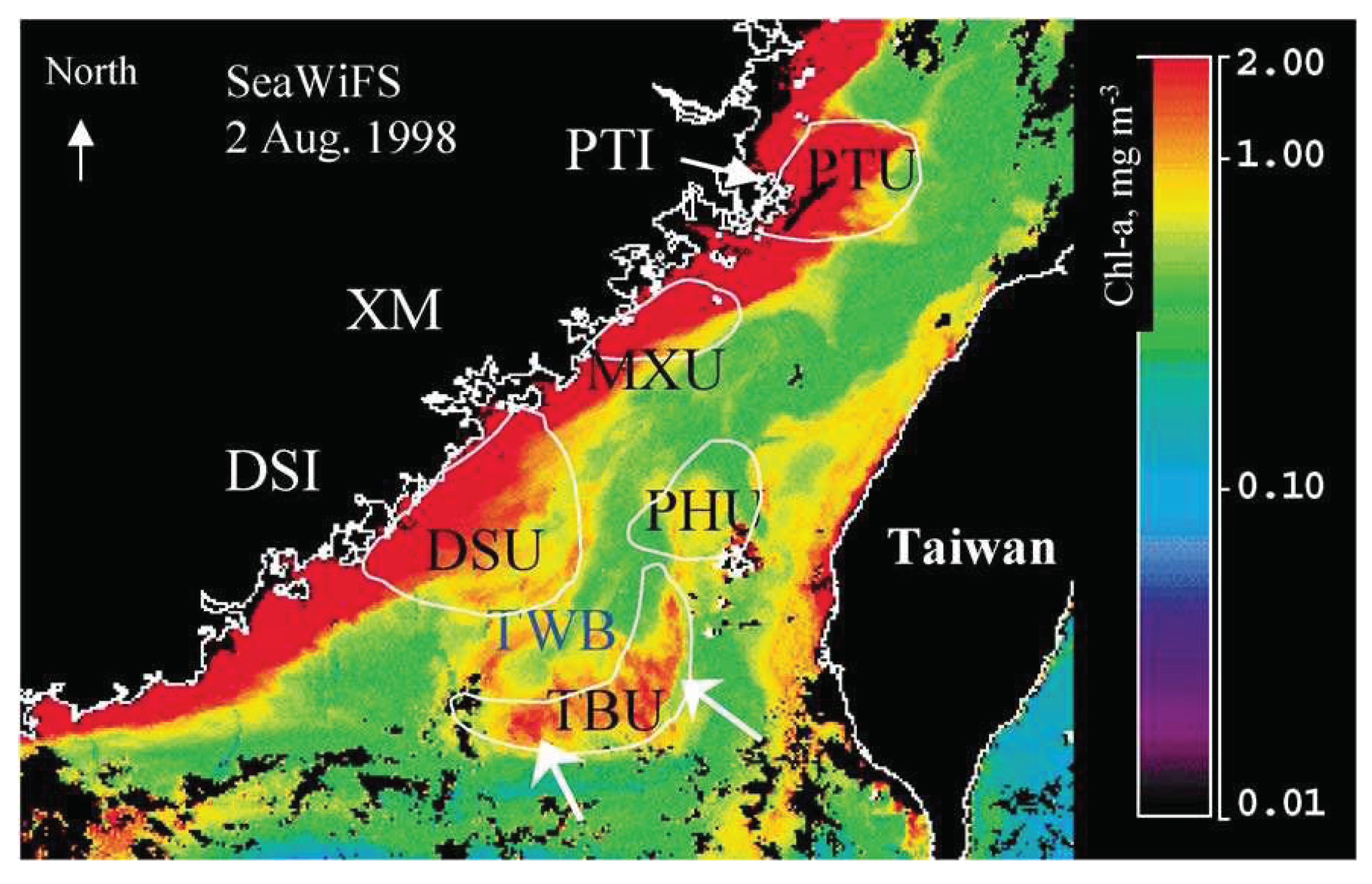
Figure 2.
Sampling stations in the waters surrounding the Taiwan Bank in October 2021 and March 2022.
Figure 2.
Sampling stations in the waters surrounding the Taiwan Bank in October 2021 and March 2022.
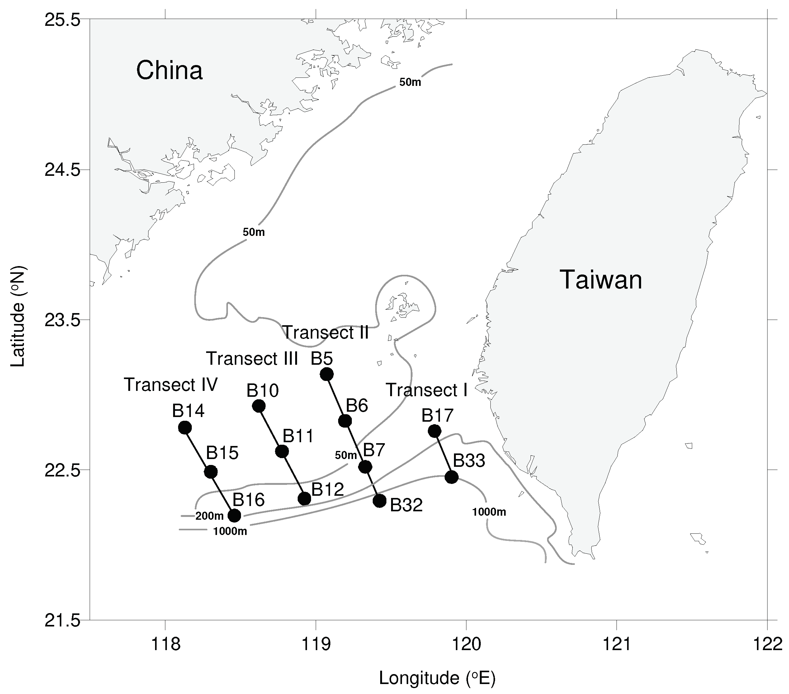
Figure 3.
Vertical profiles of temperature (°C, black lines) and salinity (gray scales) for transects II~IV in the waters surrounding the Taiwan Bank in October 2021 and March 2022.
Figure 3.
Vertical profiles of temperature (°C, black lines) and salinity (gray scales) for transects II~IV in the waters surrounding the Taiwan Bank in October 2021 and March 2022.
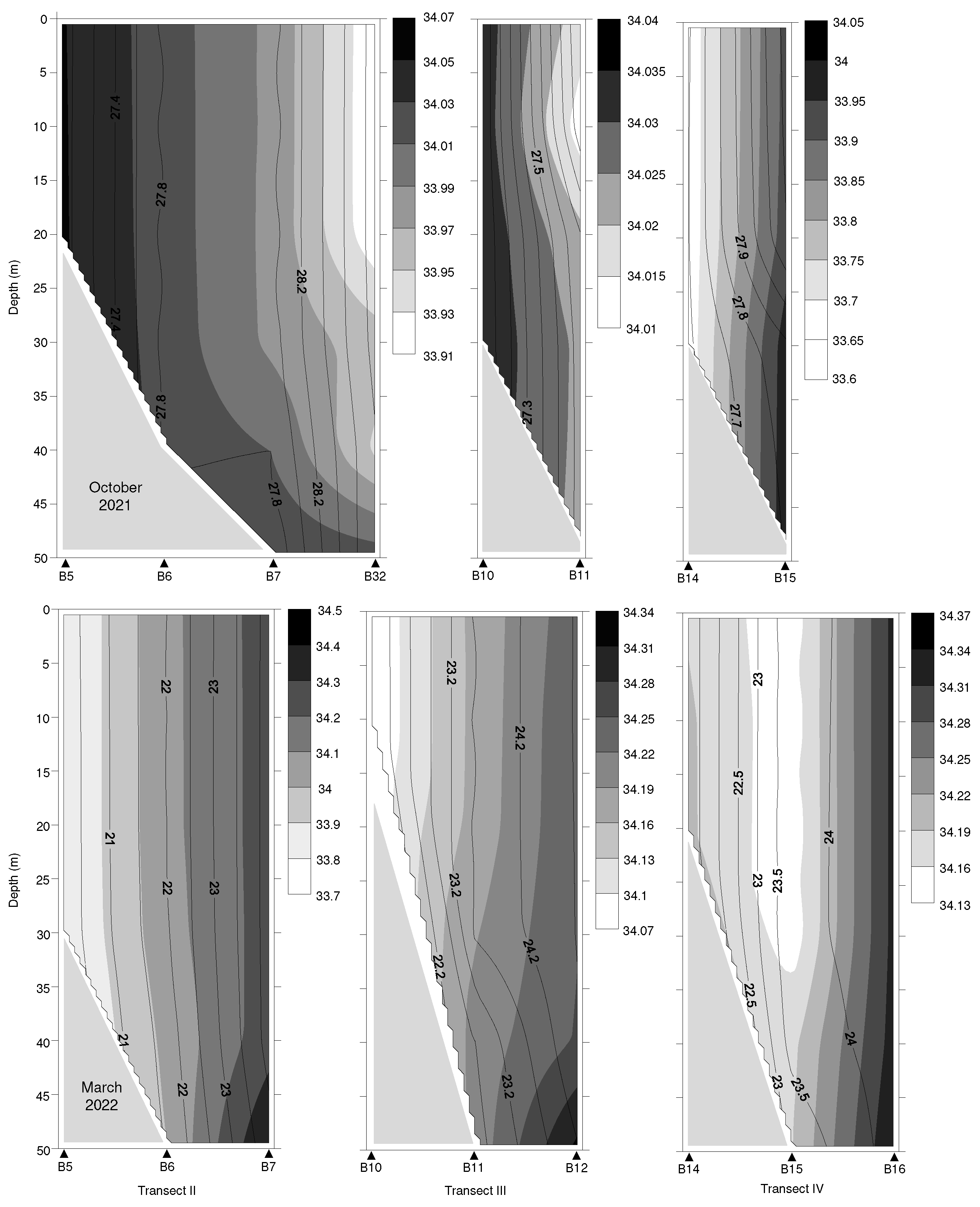
Figure 4.
Seawater fluorescence (mg m-3) at 10-m depth and zooplankton abundance (ind. m-3) in the waters surrounding the Taiwan Bank in (A) October 2021 and (B) March 2022.
Figure 4.
Seawater fluorescence (mg m-3) at 10-m depth and zooplankton abundance (ind. m-3) in the waters surrounding the Taiwan Bank in (A) October 2021 and (B) March 2022.
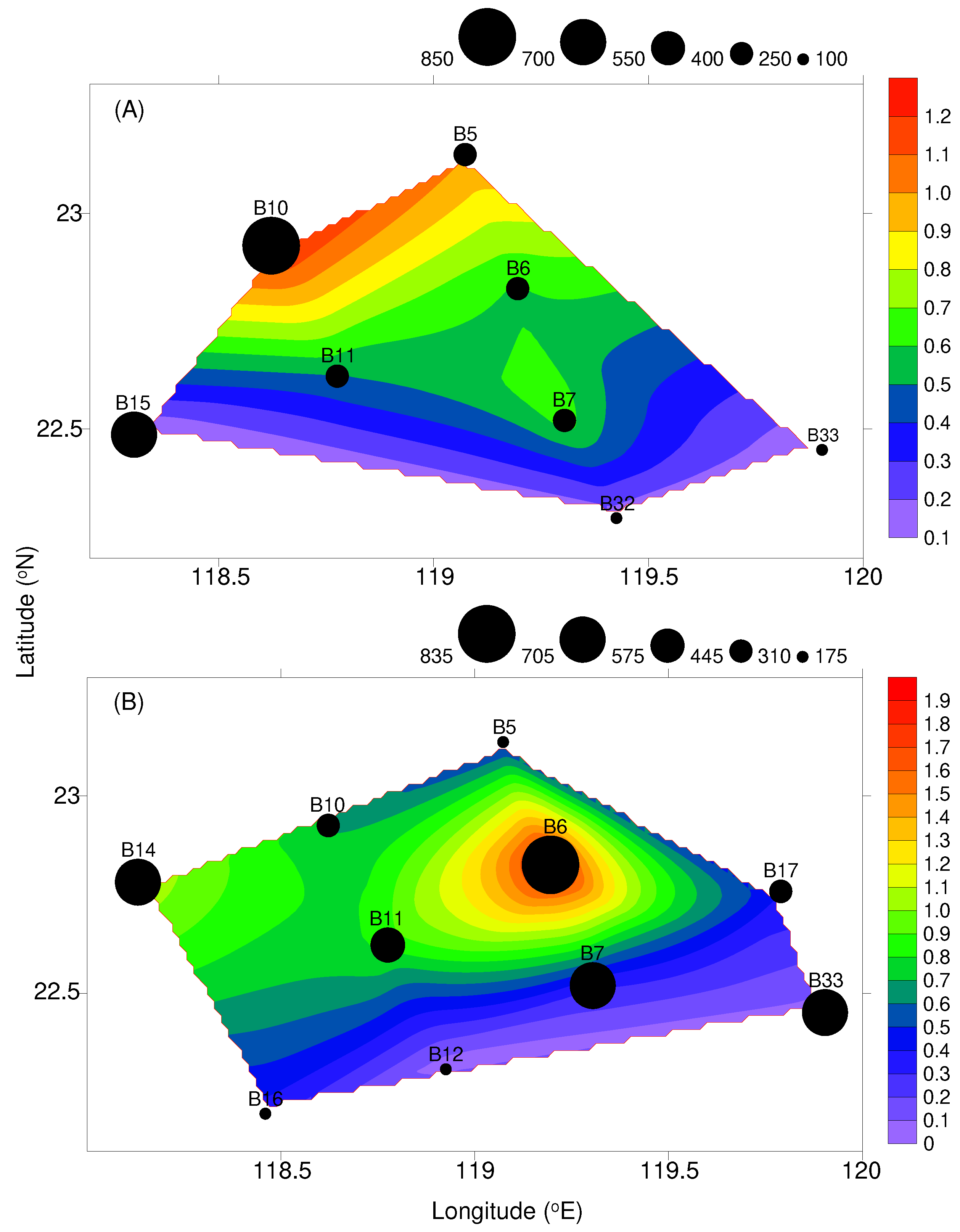
Figure 5.
Abundance of fish larvae (ind. 1000 m-3) in the waters surrounding the Taiwan Bank in (A) October 2021 and (B) March 2022.
Figure 5.
Abundance of fish larvae (ind. 1000 m-3) in the waters surrounding the Taiwan Bank in (A) October 2021 and (B) March 2022.
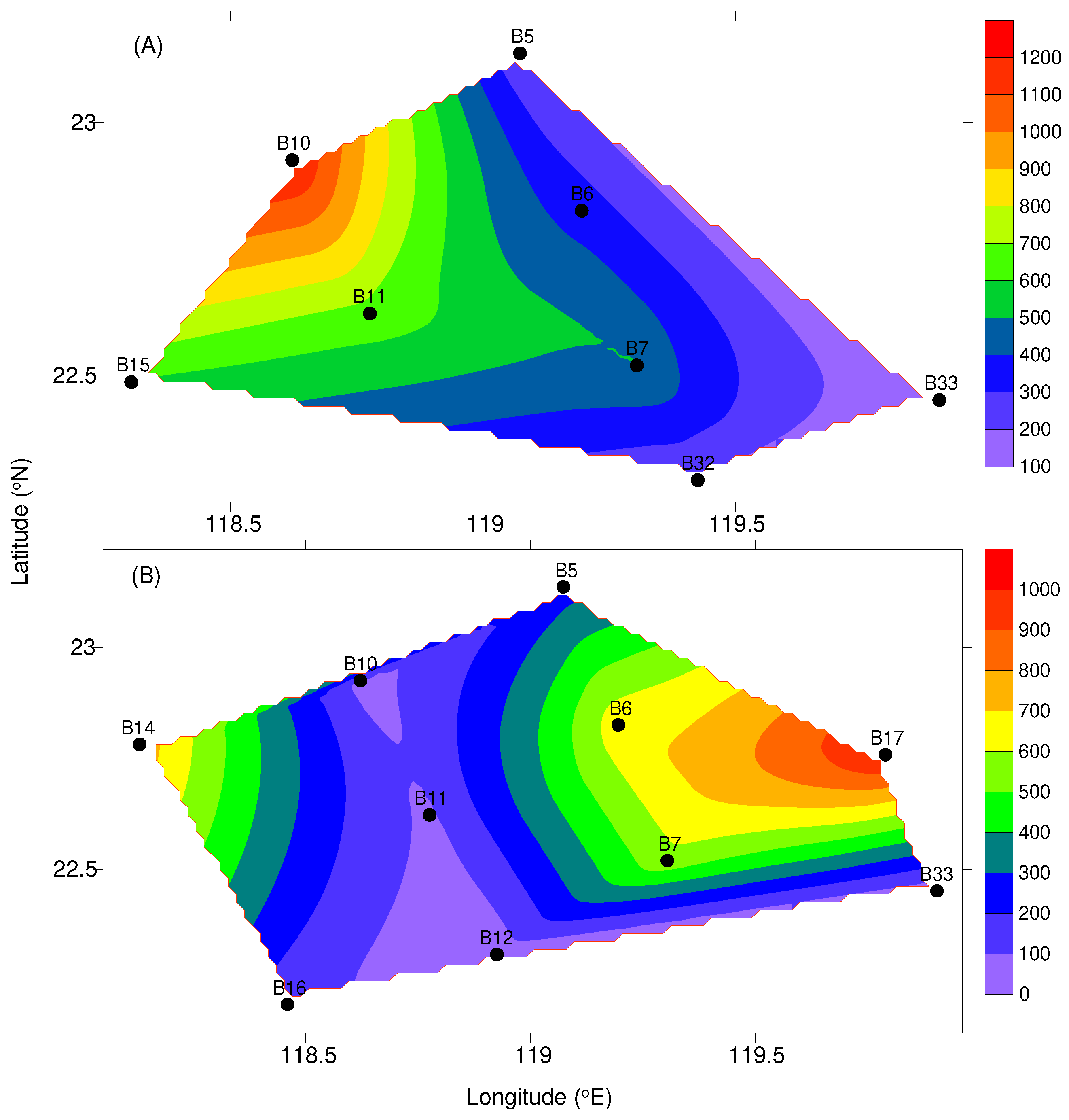
Figure 6.
Cluster dendogram and 2-dimensional MDS ordination of the Bray-Curtis similarity, based on a matrix of log(x+1)-transformed abundance of the 18 predominant taxa (>1%). Abbreviations are as follows: O = October; M = March.
Figure 6.
Cluster dendogram and 2-dimensional MDS ordination of the Bray-Curtis similarity, based on a matrix of log(x+1)-transformed abundance of the 18 predominant taxa (>1%). Abbreviations are as follows: O = October; M = March.
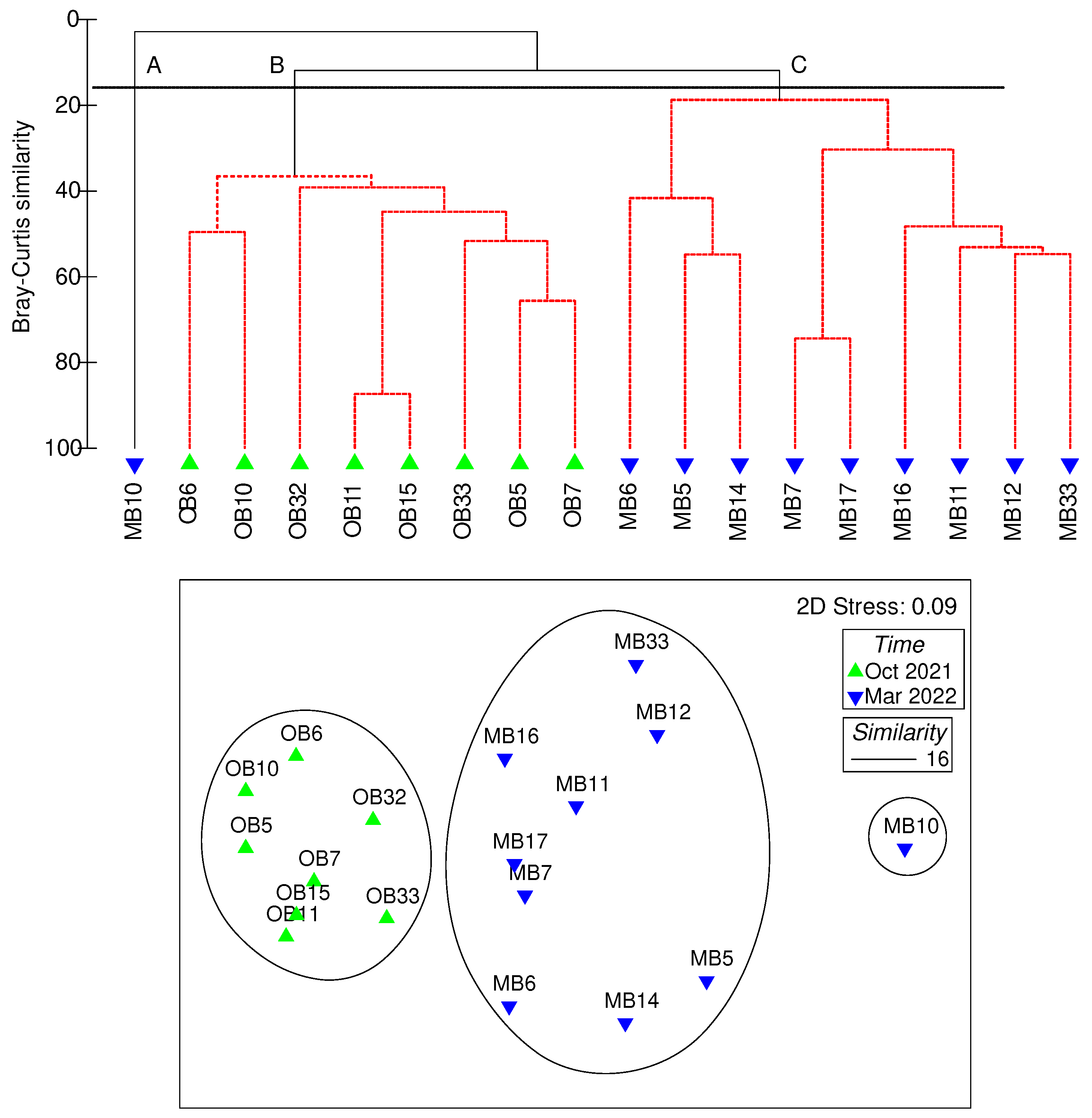
Figure 7.
Distance-based redundancy analysis (dbRDA) ordination for the composition of fish larvae constrained by the environmental variables (seawater temperature, salinity, bottom depth, fluorescence, and zooplankton).
Figure 7.
Distance-based redundancy analysis (dbRDA) ordination for the composition of fish larvae constrained by the environmental variables (seawater temperature, salinity, bottom depth, fluorescence, and zooplankton).
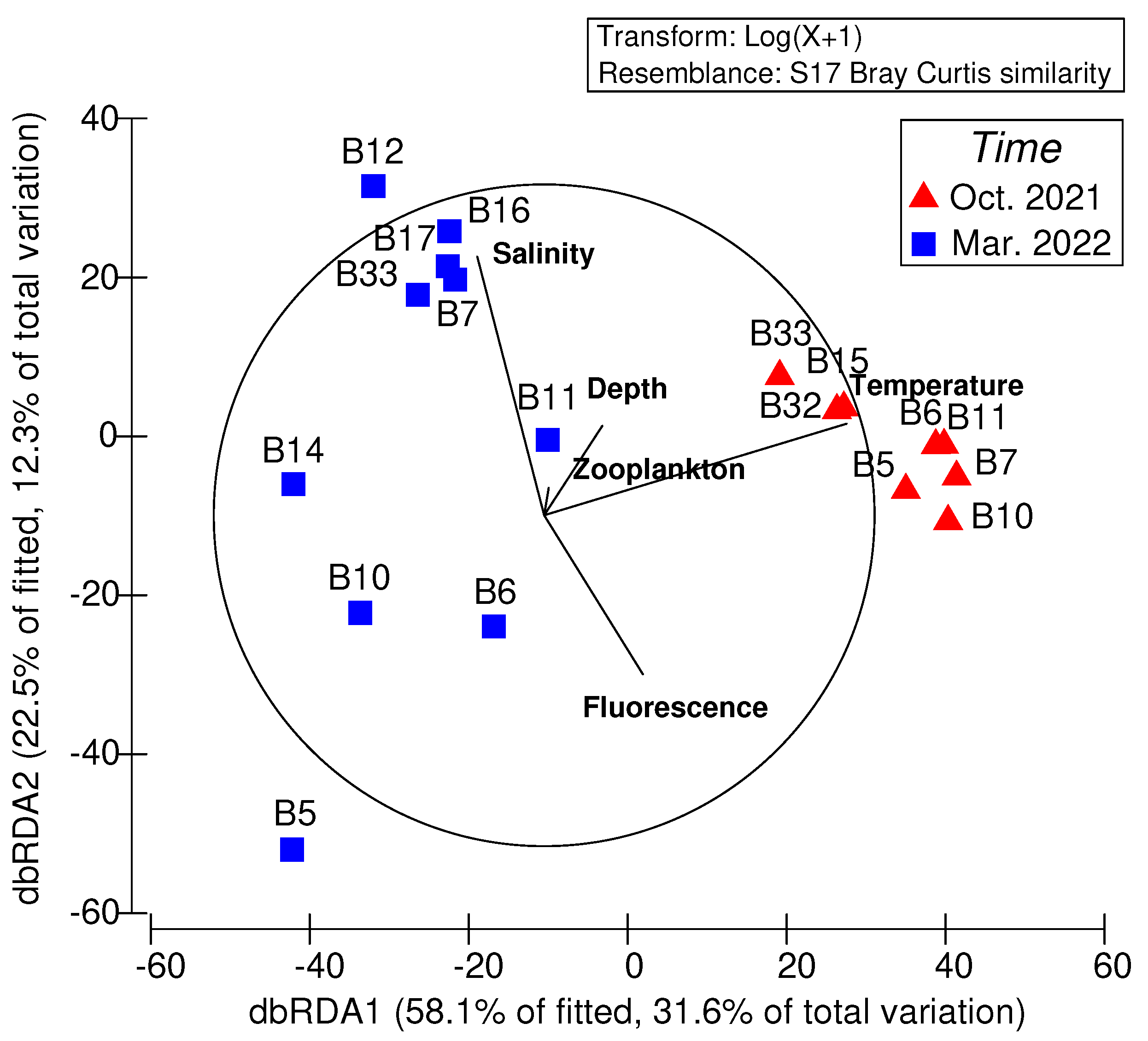

Table 1.
Mean (± SD) of four environmental variables (seawater temperature, salinity, fluorescence (at 10 m), and zooplankton abundance) and total abundance, species number, Shannon’s diversity (H’), and Pielous’s evenness (J’) of fish larvae in the waters surrounding the Taiwan Bank in October 2021 and March 2022.
| Variable | October 2021 | March 2022 |
|---|---|---|
| Environmental variables | ||
| Temperature (°C) | 27.87 ± 0.67 | 23.11 ± 1.70 |
| Salinity | 33.95 ± 0.12 | 34.15 ± 0.15 |
| Fluorescence (mg m-3) | 0.66 ± 0.51 | 0.72 ± 0.53 |
| Zooplankton (ind. m-3) | 381 ± 227 | 451 ± 226 |
| Fish larvae | ||
| Abundance (ind. 1000 m-3) | 480 ± 363 | 362 ± 364 |
| Species number (total) | 14 ± 6 (66) | 18 ± 2 (105) |
| Species diversity (H’) | 1.96 ± 0.52 | 1.99 ± 0.77 |
| Species evenness (J’) | 0.75 ± 0.14 | 0.76 ± 0.13 |
Table 2.
The most frequent captured families (> 1% of the total fish larvae) in the waters surrounding Taiwan Bank in October 2021 and March 2022.
Table 2.
The most frequent captured families (> 1% of the total fish larvae) in the waters surrounding Taiwan Bank in October 2021 and March 2022.
| Family | October 2021 | Family | March 2022 | ||
|---|---|---|---|---|---|
| Number of taxa | Contribution of family to total abundance (%) | Number of taxa | Contribution of family to total abundance (%) | ||
| Engraulidae | 2 | 26.23 | Myctophidae | 14 | 36.84 |
| Gobiidae | 5 | 16.45 | Clupeidae | 1 | 12.90 |
| Apogonidae | 1 | 14.07 | Ammodytidae | 1 | 6.88 |
| Bregmacerotidae | 2 | 9.50 | Gobiidae | 2 | 3.39 |
| Myctophidae | 10 | 8.55 | Sparidae | 5 | 3.36 |
| Trichiuridae | 1 | 3.38 | Trichiuridae | 2 | 3.09 |
| Percichthyidae | 3 | 3.16 | Mullidae | 2 | 2.84 |
| Bothidae | 3 | 1.49 | Scombridae | 6 | 2.69 |
| Sciaenidae | 2 | 1.29 | Nomeidae | 2 | 2.45 |
| Trichonotidae | 1 | 1.17 | Mugilidae | 1 | 2.21 |
| Labridae | 3 | 1.13 | Tetraodontidae | 2 | 2.09 |
| Synodontidae | 3 | 1.17 | |||
| Gempylidae | 3 | 1.11 | |||
| Pleuronectidae | 2 | 1.10 | |||
| Carangidae | 10 | 1.01 | |||
| Total | 33 | 86.41 | Total | 56 | 83.13 |
Table 3.
Mean abundance (ind. 1000 m-3) and relative abundance (RA, %) of the dominant fish larvae (>1% of the total fish larvae) in the waters surrounding Taiwan in October 2021 and March 2022.
Table 3.
Mean abundance (ind. 1000 m-3) and relative abundance (RA, %) of the dominant fish larvae (>1% of the total fish larvae) in the waters surrounding Taiwan in October 2021 and March 2022.
| Taxon | October 2021 | Taxon | March 2022 | ||
|---|---|---|---|---|---|
| Mean ± SD | RA | Mean ± SD | RA | ||
| Engraulis japonicus | 117 ± 307 | 24.38 | Diaphus slender type | 67 ± 166 | 18.38 |
| Apogon sp. | 63 ± 97 | 13.14 | Clupeidae gen. sp. | 47 ± 139 | 12.90 |
| Gobiidae gen. spp. | 56 ± 68 | 11.59 | Benthosema pterotum | 38 ± 53 | 10.42 |
| Bregmaceros sp. | 31 ± 61 | 6.41 | Bleekeria mitsukurii | 25 ± 42 | 6.88 |
| Myctophidae gen. spp. | 17 ± 15 | 3.59 | Gobiidae gen. spp. | 12 ± 28 | 3.31 |
| Tridentiger sp. | 16 ± 26 | 3.38 | Trichiurus lepturus | 10 ± 14 | 2.86 |
| Trichiurus lepturus | 15 ± 26 | 3.15 | Cubiceps pauciradiatus | 9 ± 9 | 2.39 |
| Bregmaceros nectabanus | 12 ± 20 | 2.47 | Planiliza sp. | 8 ± 17 | 2.21 |
| Notoscopelus resplendens | 11 ± 32 | 2.32 | Mullidae gen. sp. | 8 ± 20 | 2.09 |
| Lateolabrax sp. | 7 ± 18 | 1.40 | Takifugu sp. | 8 ± 16 | 2.09 |
| Percichthyidae gen. sp. | 7 ± 11 | 1.40 | Diaphus stubby type | 7 ± 16 | 1.83 |
| Asterorhombus sp. | 5 ± 14 | 1.09 | Sparidae gen. spp. | 6 ± 10 | 1.69 |
| Nibea sp. | 5 ± 15 | 1.09 | Ceratoscopelus warmingii | 6 ± 13 | 1.68 |
| Acanthopagrus sp. | 6 ± 17 | 1.52 | |||
| Myctophum sp. | 5 ± 10 | 1.34 | |||
| Scomberomorus spp. | 4 ± 12 | 1.07 | |||
Table 4.
Discriminating fish larvae taxa of three station groups based on the abundances of the top 18 dominant taxa using the SIMPER analysis that cut off for low contributions at 90%. Sim/SD: the ratio between the taxa contribution to the within-group similarity and the standard deviation; C: percentage contribution to within-group average similarity.
| Average similarity (%) | A (–) | B (43.21) | C (30.51) | |||||
|---|---|---|---|---|---|---|---|---|
| Sim/SD | C (%) | Sim/SD | C (%) | Sim/SD | C (%) | |||
| Less than two samples in group |
Gobiidae gen. spp. | 3.88 | 35.54 | Benthosema pterotum | 1.49 | 36.77 | ||
| Myctophidae gen. spp. | 1.33 | 24.89 | Cubiceps pauciradiatus | 0.66 | 33.39 | |||
| Apogon sp. | 0.64 | 12.52 | Trichiurus lepturus | 0.57 | 11.14 | |||
| Engraulis japonicus | 0.50 | 6.46 | Bleekeria mitsukurii | 0.36 | 7.54 | |||
| Trichiurus lepturus | 0.45 | 6.33 | Planiliza sp. | 0.29 | 2.91 | |||
| Tridentiger sp. | 0.49 | 5.13 | ||||||
| Total | - | 90.87 | Total | - | 91.75 | |||
Table 5.
Percentage of variation in fish larvae assemblage explained by each environmental explanatory variable included in the distance-based linear models for sampling stations. Environmental variables explaining a significant percentage of variation are denoted by asterisk; SS: sum of squares.
Table 5.
Percentage of variation in fish larvae assemblage explained by each environmental explanatory variable included in the distance-based linear models for sampling stations. Environmental variables explaining a significant percentage of variation are denoted by asterisk; SS: sum of squares.
| Variable | SS (trace) | Pseudo-F | P-value | % Variation explained |
|---|---|---|---|---|
| Temperature | 15021 | 5.8473 | 0.001* | 26.76 |
| Salinity | 7355.1 | 2.4130 | 0.026* | 13.10 |
| Bottom depth | 2663.6 | 0.7971 | 0.611 | 4.74 |
| Fluorescence | 2915.7 | 0.8767 | 0.515 | 5.19 |
| Zooplankton | 2679.5 | 0.8021 | 0.585 | 4.77 |
Disclaimer/Publisher’s Note: The statements, opinions and data contained in all publications are solely those of the individual author(s) and contributor(s) and not of MDPI and/or the editor(s). MDPI and/or the editor(s) disclaim responsibility for any injury to people or property resulting from any ideas, methods, instructions or products referred to in the content. |
© 2023 by the authors. Licensee MDPI, Basel, Switzerland. This article is an open access article distributed under the terms and conditions of the Creative Commons Attribution (CC BY) license (http://creativecommons.org/licenses/by/4.0/).
Copyright: This open access article is published under a Creative Commons CC BY 4.0 license, which permit the free download, distribution, and reuse, provided that the author and preprint are cited in any reuse.


