Submitted:
17 October 2023
Posted:
18 October 2023
You are already at the latest version
Abstract
We review the main features of the non-local gauge, named the contour gauge. The contour gauge belongs to the axial type of gauges and extends the local gauge used in the most of approaches. The geometry of gluon fields and the path-dependent formalism are the essential tools for the description of non-local gauges. The principle feature of the contour gauge is that there are no the residual gauges which are left in the finite domain of space. In the review, we present the useful correspondence between the contour gauge conception and the Hamiltonian (Lagrangian) formalism. The Hamiltonian formalism is turned out to be a very convenient framework for the understanding of contour gauges. The comprehensive comparison analysis of the local and non-local gauges advocates the advantage of the contour gauge use. As an example of practical worth, we consider the Drell-Yan process and discuss the gauge invariance of the corresponding hadron tensor. We show that the appropriate use the contour gauge leads to the existence of extra diagram contributions. These additional contributions, first, restore the gauge invariance of the hadron tensor and, second, give the important terms for the observable quantities. We also demonstrate the significant role of the additional diagrams to form the relevant contour in the Wilson path-ordered exponential. Ultimately, it leads to the spurious singularity fixing. Moreover, in the present review, we discuss in detail the problem of spin and orbital angular momentum separation. We show that in SU(3) gauge theories the gluon decomposition on the physical and pure gauge components has a strong mathematical evidence provided the contour gauge conception has been used. In addition, we prove that the contour gauge possesses the special kind of residual gauge that manifests at the boundary of space. Besides, the boundary field configurations can be associated with the pure gauge fields.
Keywords:
SU(3) and U(1) gauge symmetries
; gauge invariance
; DVCS
; contour gauge
; geometry of gluons
1. Introduction
As well-known, the gauge theories are identical to the systems with dynamical constraints where the gauge conditions (or the additional conditions in the Hamiltonian formalism) play a very significant role for quantization. Indeed, the gauge theory as the theory with the constraints can be properly quantized if and only if all constraint conditions are uniquely resolved. It should eliminate the unphysical degrees of freedom. However, the constraint conditions, which are expressed through the generalized momenta and coordinates, have very nontrivial forms. Hence, to find unique solutions of these equations is not a simple task. Even more, it sometimes becomes even impossible.
Fortunately, the Faddeev-Popov method [1] allows us to avoid the direct solution of the gauge conditions. Instead, the infinite group orbit volume leading to the quantization problems can be factorized out to the insubstantial normalization factor. It happens owing to the gauge invariance of the giving Lagrangian (or Hamiltonian) of a theory. It is, however, understood that in the spacial type of gauges the factorization of the infinite group orbit is not enough thanks to the presence of the residual gauge freedom.
Nowadays, only the local type of gauges are traditionally used for the practical applications. At the same time, one of the most popular gauge which is the axial-type gauges suffers from the residual gauge freedom. It leads to the problem with the spurious singularity. In contrast to the local axial gauge, the usage of contour gauge (we remind that the contour gauge forms the class of non-local gauges) gives a possibility to fix completely the gauge freedom in the finite region of the Minkowski (or Euclidian) space. Moreover, the fixing of residual gauges can be implemented in the most simple way and without an additional assumptions. It is worth to notice that there is, however, the residual gauge freedom at the infinite boundary of the space (see [2]).
The principal preponderance of contour gauge is that they are constructed only with the unique solution of the gauge condition from the very beginning. Namely, within the frame of contour gauge conception the gauge orbit representative should, somehow, be first fixed and, then, a certain local gauge condition, correlated with the given (gauge) orbit representative, has to be found. It is the opposite logic of the gauge fixing if compared to the usual local gauges.
Among some theorists, there is a prejudice that the study of any nonlocal gauge conditions, especially in QCD, is not attractive because the contour gauge technique is rather a specific and very complicated one. In the present review, we attempt to break this superficial and wrong impression.
To this goal, we would need the knowledge of the basic differential geometry which does not, unfortunately, receive a very wide spread in the phenomenology society. In particular, the interpretation of gluons as a connection on the principle fiber bundle are merely needed:
- to demonstrate that, within the contour gauge conception, the gauge freedom can be uniquely fixed in the finite region of the space;
- to prove that, in the local axial gauge (like ), two representations of transverse gluon fields through the strength tensor , related to the different paths of integrations integrations, and , are not equivalent each other.
We notice that stress that it is not possible to distinguish the mentioned two different representations in the local gauge. At the same time, the assumption of equivalence leads to many problems, for example, with the gauge invariance of Drell-Yan-like hadron tensors.
Since the interest to the details of contour gauge applications increases in the phenomenological community, in the review, we explain the important subtleties based on the mathematical technique adjusted to the physical language which is almost missed in literature. On the other hand, since in the recent literature one can still find a wrong representation of the transverse gluon field through the strength tensor considered in the local axial gauge, we treat this fact as a strong motivation for the present review.
To demonstrate the practical profits of the contour gauge conception, in the review, we are focusing on the investigation of nucleon (hadron) composite structure which is still the most important subjects of hadron physics. In particular, we dwell on the calculation of several sorts of the single spin asymmetries (SSA). From the experimental point of view, SSAa are the wide-spread and useful instruments for such studies and they open the access to the three-dimensional nucleon structure. It takes place thanks for the non-trivial connection between the transverse spin and the parton transverse momentum dependence (see, for example, [3,4,5,6,7]) In QCD, SSA related to the Drell-Yan (DY) process was first considered in the case of the longitudinally polarized hadron [8,9]. This SSA is important because the second hadron is a pion. It is necessary to mention on the sensitivity to the shape of pion distribution amplitude, being currently the object of major interest [10,11,12,13] (see also [14] and the references therein). In [8,9,10,11], it was shown that the imaginary phase of SSA, which is associated with the longitudinally polarized nucleon, appears due to either the hard perturbative gluon loops or twist four contribution of the pion distribution amplitude.
Previously, in the study of transverse SSA of DY process, the imaginary part has been only extracted from the quark propagator in the standard diagram (that is, the diagram without radiations from the quark legs in the correlators) with quark-gluon twist three correlator [15]. In these approaches, the ambiguity in the boundary conditions for gluons provide the purely real quark-gluon function which parameterizes matrix element. On the other hand, the real -function kills the contribution from the non-standard diagram (that is, the diagram with radiations from the quark legs in the correlators) which is, however, absolutely necessary to ensure the QED gauge invariance of the DY hadron tensor. To resolve this discrepancy, in the series of papers [16,17], with the help of the contour gauge conception, it has been proven that the twist three -function is, in fact, the complex function. With this inference, the non-standard diagram does give the non-zero contribution and does produce the imaginary phase required to have the SSA. Besides, the additional contribution of the non-standard diagram also leads to an extra factor of 2 for SSA.
The other motivating point for the development of the contour gauge formalism is related to the problem of the spurious singularity fixing (see, for example, [7,18,19]). The light-cone axial gauge condition imposed on gluon fields, , naturally enables the parton number (probability) interpretation of parton density functions in the tree level [20]. However, any perturbative calculations beyond the tree level demand the careful treatments of the spurious uncertainties in gluon propagators [21,22,23,24]. It is worth to remind that the spurious singularities arise as ill-defined pole singularities of the form like . Basically, they are associated with the residual gauge freedom due to incomplete gauge fixing by . For this reason, the direct calculations in the axial light-cone gauge in higher perturbative orders are cumbersome and sometimes even contradictory [25,26]. From one hand, one would try to overcome this difficulty by working in the well-defined general covariant gauge setting the gauge parameter to , which is known to effectively `imitate’ non-covariant gauges [26,27]. Or, from the other hand, we would follow another approach to keep working in the light-cone gauge and to get rid of the residual gauge freedom by an appropriate extra gauge-fixing condition. The latter can be obtained in terms of the various boundary conditions for the gluon fields and/or their spatial derivatives [7,18,19].
In the present review, we give the detail description of an alternative approach to formulation of the more general gauge-fixing condition from the very beginning. It is supposed to entail the “right” pole prescriptions for the gluon propagator. With the help of the contour gauge conception, we demonstrate how the spurious uncertainties in the gluon propagator can ultimately be fixed in the nonlocal axial gauges. Within the framework of collinear factorization, we specially emphasize the substantial role of the nonstandard diagram to get the relevant contour in the Wilson path-ordered exponential needed to fix ultimately the spurious singularity in the gluon propagator.
The other demonstrative example of the practical profits presented in the review is given by the problem of separation of the parton spin and orbital angular momentum (AM). It is one of interesting subjects of modern disputes in both the theoretical and experimental communities [28]. Nowadays, two concurrent decompositions, as known as Jaffe-Manohar’s decomposition (JM-decomposition) [29] and Ji’s decomposition (J-decomposition) [30], have widely been discussed. The JM-decomposition refers to a complete decomposition of the nucleon spin into the spin and orbital parts of quarks and gluons individually. While, the J-decomposition possesses the gauge invariance by construction but, at the same time, it does not lead to the separable quark and gluon contributions of spin and orbital AMs to the whole nucleon spin.
In [31,32], the gauge invariant analogue of JM-decomposition has been proposed. Considering the Coulomb gauge condition, they have advocated that the gluon field can formally be presented as . It is worth to notice that this decomposition has being assumed as the fist-step ansatz in all existing discussions on the gauge-invariant separation of spin AM from the orbital AM (see, for example, [33,34,35,36,37,38,39,40,41,42,43,44]).
In the Abelian gauge theory the physical components correspond to the transverse components which are gauge invariant in contrast to the longitudinal components associated with which are gauge-transforming and they should be eliminated by the gauge condition used in the Lagrangian approach. As a result, in the Abelian theory, the mentioned decomposition is absolutely natural and there is no doubt of its validity at all.
In the non-Abelian gauge theory, both the transverse and longitudinal components are gauge-transforming. Hence, the mentioned decomposition is actually questioned regarding the definition of the physical components. In particular, the use of covariant-type gauge conditions should inevitably lead to the inability to separate the spin and orbital AMs in the gauge-invariant manner because the coordinate dependence of gluon configurations cannot be independently determined for every of components, see for example [45]. Meanwhile, the decomposition plays a role of keystone in many discussions devoted to the gauge-invariant separation of spin AM from orbital AM.
In the review, we propose to consider the gluon decomposition as a statement which must be proven, if it is possible, within the non-Abelian theory. It turns out that the proof can be implemented and elucidated only with the help of the contour gauge conception (cf. [46,47]). It is necessary to remind that the contour gauge can be readily understood in the frame of the Hamiltonian formalism where the contour gauge condition defines the manifold surface crossing over a group orbit of the fiber uniquely (see [48] for further details). Also, it is demonstrated that even in the contour gauge one can deal with a special kind of the residual gauge freedom. However, this residual gauge is located in the nontrivial boundary pure gauge configurations defined at infinity.
Notice that the physical quantities do not depend on the choice of gauges, as it must be. The axial type of gauges is related to the certain fixed direction in a space. In this particular case, the gauge independency should be treated as an independency with respect to the chosen direction which is ensured by additional requirements [49].
2. The Contour Gauge in Use: The General Principles
2.1. The Lagrangian and Hamiltonian Systems with the Dynamical Constraints
The local axial gauge, , suffers from the residual gauge freedom. Hence, it demands the additional requirements to fix the remained gauge freedom. In the most of cases, the formulation of additional requirements is not a trivial task within the Lagrangian system. Indeed, if one demands simultaneously , the maximal gauge fixing is available only in a classical theory. In a quantum theory, the simultaneous conditions and as delta-function arguments in the corresponding functional integration (which lead to the effective Lagrangian with and ) result in the absence of the well-defined gauge propagator. It happens because the corresponding kinematical operator cannot be inverted. In this connection, it is necessary to develop an alternative method of gauge fixing compared to the “classical” approaches with the effective Lagrangian including both and . The contour gauge conception gives us such an alternative and effective method.
In order to understand all subtleties of the contour gauge, we remind the main stages of the Lagrangian (L-system) and Hamiltonian (H-system) approaches to the quantization of gauge fields (see, for example, [50]). In this section, our efforts are concentrated on the demonstration that the H-system is the most adequate approach for our purposes. At the same time, due to the special role of a time-space in H-system, the L-system is more suitable for a practical use. In other words, we need the H-system as a convenient intermediate instrument to see how the contour gauge fixes uniquely the total gauge freedom. However, the main computation procedure has been formulated in terms of L-system related, of course, with the corresponding H-system.
Let us consider the H-system, defined by , where the phase space is formed by the generalized momenta and coordinates . In addition, we have constraints on and which have been imposed on the system. Traditionally, these constraints are denoted by and .
We suppose that the H-system has an equivalence orbit which is nothing but the gauge group orbit in the gauge theory. Since the phase space is overfilled by unphysical degrees, in the ideal case, we have to resolve all kinds of constraints. The additional constraints are necessary to fix uniquely the orbit representative. It is needed to quantize the H-system. From the pure theoretical viewpoint, after resolving all constraints we deal with the quantized H-system where the physical phase space of dimension is a subspace of the initial space of dimension . It is a fundament for H-system in terms of physical configurations, .
In the functional method of quantization, the amplitude between the initial and the final states takes the form of (modulo the unimportant normalization factors) [1,50]
where denotes the Poisson brackets.
The delta-function of Eqn. (1) can be presented through the integration over the Lagrange factor as
It gives the generalized Hamiltonian of system which reads
If we suppose that the constraint conditions (see the delta-function arguments) have somehow been resolved, the amplitude is given by
where only the physical generalized momenta and coordinates are forming the integration measure together with the Hamiltonian. The generating functional of (4) corresponds to the H-system with the dynamical constraints which have been resolved. Therefore, there is no a (gauge) freedom associated with the arbitrary Lagrange factor . It would be an ideal situation which cannot be realized practically in the most of cases. However, the contour gauge, as a class of nonlocal gauges, gives a possibility to realize the mentioned ideal situation. It is so because the contour gauge condition has a unique solution by construction, see below.
It is instructive to illustrate the difference between the H-system with unresolved and resolved constraint conditions. It can be done with the help of a trivial mechanical example, see Figure 1. Consider the homogenous flat “ball” which moves from the point A to the point B. The ball has a spherical symmetry under the rotation around the inertia center. For the sake of simplicity, we focus on the ball rotation in a two-dimensional plane. Since the flat ball surface is homogenous, we do not have a chance to observe the rotation of the moving ball unless we mark some point on the surface. The invisible ball rotation around its center of inertia corresponds to the inner (gauge) transformations of the H-system. It does not affect much the trajectory provided the angle velocity is constant, see the left panel of Figure 1. In this case, the inertia center plays a role of “physical” configurations of the H-system, while the moving of different sites on the flat ball surface is invisible and relates to the “unphysical” configurations.
If we mark the site on the flat ball surface by a dash, we break down the rotation symmetry. It means that we choose, so to say, the preferable site of the ball surface and the ball rotation becomes visible. In this case, we can describe the moving dash together with the inertia center as “physical” configurations of the H-system when the ball position varies from A to B, see the right panel of Figure 1.
In the context of the contour gauge conception, the marked dash on the flat ball corresponds to the certain gauge function of the gauge transformations which has been fixed by the contour gauge condition. If we focus on the above mentioned ideal case of resolved constraints, we would merely deal with the gauge fields considered as a massless vector fields (transforming as a spinor of 2-rank under the Lorentz group) that are described by the Hamiltonian without the gauge transforms.
In both the Abelian and non-Abelian gauge theory, the correspondences between the canonical variables and the dynamical constraints (cf. Eqn. (1)) can be expressed as
In the typical gauge theories, resolving the additional (or gauge) conditions is not a simple task. The gauge conditions, leading to the equation system for the gauge function , would have an unique solution . In fact, it might be practically impossible.
Within the frame of L-system, Faddeev and Popov have proposed the method (FP-method) to avoid the needs for finding the unique solution . In FT-method, the infinite group orbit volume can be factorized out to the insubstantial normalization factor. It becomes thanks to the gauge invariance of the corresponding Lagrangian (or Hamiltonian) of theory [1].
For the simplicity, let us dwell on gauge theory. The H-system can be readily stemmed from the Lagrangian formalism of first order. The Lagrangian of first order is defined by
where and are supposed to be independent field configurations. The Lagrangian of Eqn. (6) can be written in 3-dimensional form. We have
where and imply the generalized momenta and coordinates, respectively. Besides, are the implicit variables in the integration measure, see below. From the Euler-Lagrange equations we can get the equations which do not include . These equations give the constraint conditions written in the forms of
The gauge theory can be considered as the theory with the constraints which are applied on the field configurations. The constraint conditions of Eqn. (8) have to be completed by the additional (or gauge) conditions. For example, they read
The full set of conditions defined by Eqns, (8) and (9) should eliminate all unphysical degrees of freedom for the correct quantization of H- (or L-) system.
Using the FP-method, we begin with the functional integration written for the L-system [50]. We have
where the infinite group orbit volume given by has been factorized out in the integration measure due to the gauge invariant action and functional .
The exact magnitude of the group volume prefactor, i.e.
is irrelevant because the prefactor should be cancelled by the corresponding normalization of Green functions. In Eqn. (11), the infinite group volume corresponds to the standard case of unresolved gauge conditions. The zero group volume appears in the case of resolved gauge conditions. Indeed, the integration measure can be defined on the group manifold as an invariant measure,
denotes the product of the invariant measures defined on the structure group G of fiber over each point of the Minkowski space. If the gauge function is not fixed, we have the infinite integration over the group invariant measure, otherwise (that is, if the gauge function is somehow fixed) the integration is equal zero for each point of the Minkowski space but the value of fixed can vary from one point to another.
Returning to Eqn. (10), it can be identically rewritten as
where the functional of action is given by the Lagrangian of Eqn. (6). In the three-dimensional forms, we obtain that
where is now defined by Eqn. (7). Integrations over and in Eqn. (14) lead to the functional integral which is given by
where the Hamiltonian is
In Eqn. (15), the gauge condition is chosen to be .
On the other hand, Eqn. (15) can be presented in the equivalent form. It reads
where the primary and secondary constraints together with the gauge conditions of Eqn. (9) have been explicitly shown in the functional integrand. This representation of H-system resembles the functional integration presented by Eqn. (1).
Notice that, in H-system, there are no problems to write all constraints through the delta functions. It is true because, in contrast to L-system which is forming the Feynman rules, we have no needs to invert the kinematical-like operator. At the same time, the H-system approach is not convenient for the practical computation in QFT.
This section is basically written in the textbook style. The basic reason for the usage of this style is that the section is preparing a reader for the main features of contour gauge uses. Indeed, we have reminded the differences between the H-systems with and without resolved additional dynamical constraints presenting the mechanical illustration in Figure 1. Within the FP-method of L- and H-systems there is no need to find a unique solution of the additional (gauge) condition system with respect to the gauge function . Thanks for the gauge invariance of Lagrangian (Hamiltonian) and functional , the infinite group orbit volume defined by has been factorized out in the corresponding functional integration measure giving a possibility to quantize the gauge theory modulo the residual gauge problems. However, if we resolve the additional (gauge) condition with respect to , the group representative on each of orbits can be fixed uniquely. The factorized group integral defined through the Riemann summations should be equal to zero. Since the group volume has been cancelled by the corresponding normalization, it does not mean that the functional integration of Eqn. (10) disappears. This case takes place if we use the contour gauge conception.
2.2. The Contour Gauge Conception
We now concentrate on the description of the contour gauge conception. It implies that the corresponding gauge condition can be formally resolved in order to find the unique gauge orbit representative. A few decades ago, the contour gauge had intensively been studied due to the fact that the quantum gauge theory should not suffer from the Gribov ambiguities (see, for example, [46,47,51]).
It states that the gauge function can be completely fix (in the H-system, see Eqn. (1)). In other words, the unphysical gluons can be eliminated (in the L-system, see Eqn. (10)) if we demand the path dependent functional (Wilson path functional) to be equal to unity, i.e.
where the path between the points and x is fixed.
In QCD, the axial light-cone gauge, , is a particular case of the reduced nonlocal contour gauge, see below, determined by Eqn. (18) if the fixed path is given by the straightforward line connecting with x. By construction, the contour gauge does not possess the residual gauge freedom in the finite space. In [2], it is shown that the possible residual gauge can be located at the corresponding boundary only. In what follows the boundary gluon configurations have assumed to be equal to zero. So, from the technical point of view, the contour gauge provides the simplest way to fix the gauge function completely.
The contour gauge conception is inspired by the path group formalism [52,53]. Also, it can be traced from the Mandelstam approach [54]. For better understanding, it is worth to give a short introduction to the geometry of gluons where the gluon field has been treated as a connection on the principle fiber bundle .
The principle fiber bundle is one of main ingredients that forms a differential geometry basic. By definition, it is a combination of two sets, and together with the given transformations between them. Moreover, the group structure G is determined on the set (strictly speaking, on each of fibers). The set is named by a base of the fiber bundle. The base usually coincides with the Minkowski space. In the principle fiber bundle, we are able to define two directions. One direction is determined in the base as the tangent vector of a curve going through the point . The other direction is defined in the fiber and can be uniquely determined as the tangent subspace related to the parallel transport [52,53]. These two directions allow us to introduce the horizontal vector defined by
where denotes the corresponding shift generator along the group fiber written in the differential form. The vector coefficients (connection of the principle fiber bundle), , defines the algebraic vertical (tangent) vector field on the fiber [52,53]. The horizontal vector is invariant under the structure group G acting on the given representation of the fiber by construction.
In , the functional of Eqn. (18) is a solution of the parallel transport equation given by
where the fiber point with the curve parametrized by s. Eqn. (20) being a differential equation takes place even if is fixed on the group. it is true because, in this case, while . In this connection, the condition presented by Eqn. (18) implies that the full curve-linear integration goes to zero rather than the integrand itself.
It can be shown [52,53] that every of points belonging to the fiber bundle, , has one and only one horizontal vector corresponding to the given tangent vector at . We remind that the tangent vector at the point x is uniquely determined by the given path passing through x. In the frame of H-system based on the geometry of gluons the condition of Eqn. (18) corresponds to the determining of the surface on that is parallel to the base plane with the path. Moreover, it singles out the identity element, , in every fibers of , see Figure 2. This choice can be traced to the Lagrange factor which is formally fixed in H-system, see Section 2.1. Roughly speaking, once the group (any) element of fiber is fixed, we deal with the Lagrange factor of H-system which is also uniquely fixed. On the other hand, if we fix the group element of fiber we fix the function theta of gauge transforms as well. In this sense, we do not have the local gauge transforms (or the gauge freedom) anymore.
The path dependent functional given by the l.h.s. of (18) can be also gauge transformed. We have
where the local gauge function defined by
with the corresponding generator . From this, one can see if the Minkowski space has been realized as a loop space, the path dependent functional becomes invariant under the local gauge transforms. In the general case of arbitrary paths, imposing the condition (18) on the r.h.s. of (21), we are able to get the different contour gauge with , see (22). From the theoretical point of view, this new contour gauge has the same status as the gauge of (18). It would correspond to the different plane in Figure 2 which also transects the principle fiber bundle and, therefore, it generates the different contour gauge condition which, generally speaking, is related to the previous contour gauge by the local transform. However, from the practical point of view, the contour gauge given by is not convenient to use for calculations because the representation of transverse gluon field through the strength tensor has a more complicated form compared to, for example, (53). Of course, the physical quantities are independent on the contour gauge choice.
Notice that since the gauge condition given by Eqn. (18) selects only the identity element of group G on each fiber, it means that the gauge transforms have been reduced to the “global” gauge transforms. That is, the gauge function becomes the coordinate independent and is fixed . This situation is identical to that one can see in Figure 1 of Section 2.1. Namely, the red dash on the ball surface corresponds to one particular choice of the group element fixed by the given contour gauge. However, if we mark the line on the ball surface by the other dash, it would mean that we choose the other group element fixed by the different contour gauge. In both cases, we deal with the same description of H-system.
Since the functional depends on the whole path in , the contour gauge refers to the non-local class of gauges and generalises naturally the familiar local axial-type of gauges. It is also worth to notice that two different contour gauges can correspond to the same local (axial) gauge with the different fixing of residual gauges [16,17]. If we would consider the local gauge without the connection with the non-local gauge, the residual gauge freedom would require the extra conditions to fix the given freedom. This statement reflects the fact that, in contrast to the local axial gauge, the contour gauge does not possess the residual gauge freedom in the finite region of a space where the boundary gluon fields are absent [2].
2.3. Comparison of Local and Nonlocal Gauge
The contour gauge as a nonlocal kind of gauges generalizes or extends the standard local gauge of axial type. Therefore, it is worth to discuss shortly the correspondence between the local and nonlocal gauge transforms.
Let us begin with the axial local gauge defined by . The nonlocal gauge is given by Eqn. (18) and the local gauge can be obtained from Eqn. (18) if, as above-mentioned, the starting point is and the path is fixed to be a straightforward line, . The differences between the local and nonlocal gauges can symbolically be demonstrated by the following trivial example. Consider two different vectors A and B. We stress that they are different by construction. We now assume that these vectors have the same projection on the certain direction given by another vector N. It is clear that if the vectors have the same projections on the vector N, it does not mean the equivalence of vectors A and B, i.e.
In this example, the different vectors A and B can be associated with two different contour nonlocal gauges,
While the local axial gauge plays a role of the projections on N,
On the other hand, focusing on only the N vector projection, there is no additional information to see from which vectors A or B the given projection has been performed.
We are coming back to the local axial gauge. The local axial gauge suffers from the residual gauge transformations which can lead to the spurious pole uncertainties. However, the preponderance of nonlocal (contour) gauge is that it fixes all the gauge freedom in the finite space (see for instance [2]). To demonstrate it in the simplest way, we consider the local axial gauge as an equation on the gauge function . We have
where with . We can readily find a solution of this equation which takes the form of the undetermined integration given by
At the same time, the solution can be rewritten via the determined integration, it reads
Here, is fixed and is an arbitrary function which does not depend on . is given by
The arbitrariness of C-function also reflects the fact that we deal with an arbitrary fixed starting point .
Let us study the residual gauge freedom requiring both and , we then have
One can see that the function C determines the residual gauge transforms. This situation takes place in the local axial gauge defined by the only condition applied for (28).
We go over to the nonlocal gauge which actually gives more information on the gauge fixing. The nonlocal (contour) gauge extends the local axial-type gauge and it demands that the full (curve-linear) integral in the exponential of Eqn. (18) has to go to zero. We stress that in contrast to the local gauge where the corresponding exponential disappears thanks to that the integrand goes to zero. One can demonstrate it on the example of solutions (27) or (28). Indeed, in the contour gauge the residual gauge function can be related to the path dependent functionals with and which are also disappeared eliminating the gauge freedom and giving the physical gluon representation in the form of (134) (see [18,55] for details). That is, if we restore the full path in the path dependent functional for a given process, we can get that
Then, requiring the conditions as
we get that
In the contour gauge, Eqn. (34) means that no the gauge freedom has left at all. We emphasize that the condition of (32) demands that the integrand is zero, while the condition of (33) is imposed on the integration which leads to the corresponding representation for the transverse gluon field, see (53), (54) and (134). Besides, the exact value of the fixed starting point depends on the process under our consideration [18].
The path dependent functional also defines the path dependent gauge transformation in the form of
where the starting point is now fixed. Hence, having calculated the derivative of in (35), we get that (here, for the simplicity, )
where . If we are now focusing on the case of , we readily obtain that the gluon representation reads
where the traditional notations
have been introduced. The representation given by (37) is an important result for our further considerations.
So, in this section, we have demonstrated that the contour gauge gives a possibility to illuminate the unphysical gluon components, meanwhile the local axial gauge fixes the gauge partially leaving room for the residual gauge freedom.
2.4. The Advantages of the Contour Gauge Use
In the subsection, we concentrate our attention on the certain examples which, first, relate to the practical use of the contour gauge and, second, demonstrate the preponderance of the nonlocal gauges compared to the local gauges.
As discussed in [16,17,55], the Drell-Yan-like processes with the polarized hadrons give the unique example where the contour gauge use shows the definite advantage from the practical point of view. In particular, the contour gauge use allows to find the new contributions to the Drell-Yan-like hadron tensor which restore and ensure the gauge invariance of the corresponding hadron tensors [16,17,55]. It is important, however, to stress that the mentioned new contributions are invisible if we would work within the frame in the local gauge.
In the similar manner, due to the contour gauge conception the -process of DVCS-amplitude which clarifies the gauge invariance of the non-forward processes takes the closed form again [56]. From the practical point of view, it is instructive to consider the appearance of standard and non-standard diagrams contributing to the well-known deeply virtual Compton scattering (DVCS) amplitude in the frame of the factorization procedure. The gluons radiated from the internal quark of the hard subprocess generate the standard diagrams, while the non-standard diagrams are formed by the gluon radiations from the external quark of the hard subprocess (see [56] for details).
In the most cases, it is sufficient to exponentiate only the longitudinal components of gluon field, and , which are related to the unphysical degrees. Indeed, the standard diagram contributions give the gauge invariant quark string operator which reads
where
and stands for -matrices the exact form of which is now irrelevant.
The non-standard diagram contributions result in the string operator defined as
where
Hence, using the contour gauge conception, we eliminate all the Wilson lines with the longitudinal gluon fields and demanding that
and
Eqns. (45) and (46) give rise to the local gauge conditions given by and .
With respect to the Wilson line with the transverse gluons , we remind that we work here within the factorization procedure applied for DVCS-amplitude. In this case, the Wilson lines with the transverse gluon fields are considered in the form of an expansion due to the fixed twist-order, and the transverse gluons correspond to the physical configurations of L-system.
Thus, the DVCS process gives us the example how the unphysical gluon degrees can be illuminated from the consideration with the help of contour gauge.
We are now going over to the Drell-Yan (DY) process with one transversely polarized hadron [16]
where the virtual photon producing the lepton pair () has a large offshelness, i.e. , while all the transverse momenta are small and integrated out in the corresponding cross-sections . Here, the contour gauge use results in the gauge invariant hadron tensor and provides the new contributions to single spin asymmetries. Having considered this hadron tensor in the asymptotical regime associated with the very large , the factorization theorem can be applied for the given hadron tensor as well as for the DVCS process. As a result, the DY hadron tensor takes a form of convolution as
where both the hard and soft parts should be independent of each other and are in agreement with the ultraviolet and infrared renormalizations. Moreover, the relevant single spin asymmetries (SSAs), which is a subject of experimental studies, can be presented as
where and are the lepton and hadron tensors, respectively. The hadron tensor includes the the polarized hadron matrix element which takes a form of
where stands for the Fourier transform between the coordinate space, formed by positions , and the momentum space, realized by fractions ; the light-cone vector is a dimensionful analog of n. In Eqn. (50), the parametrizing function B describes the corresponding parton distribution.
In the studies, see for example [7,57,58,59], where the local light-cone gauge has been used, B-function of Eqn. (50) is given by a purely real function. That is, we have
where the function parametrizes the corresponding projection of and obeys .
In Eqn. (51), the pole at is treated as a principle value and it obviously leads to . Indeed, within the local gauge , the statement on that B is the real function stems actually from the ambiguity in the solutions of the trivial differential equation, which is equivalent to the definition of ,
The formal resolving of Eqn. (52) leads to two representations written as
We stress that within the approaches backed on the local axial gauge use, there are no evidences to think that Eqns. (53) and (54) are not equivalent each other. That is, the local gauge inevitably leads to the following logical scheme (see [17] for details)
This equation demonstrates that the equivalence of Eqns. (53) and (54) causes the representation of B-function as in Eqn. (51). The discussion on the boundary configurations can be found in [17].
Regarding the DY process, the physical consequences of the use of B presented by Eqn. (51) are the problem with the photon gauge invariance of DY-like hadron tensors and the losing of significant contributions to SSAs [16,17]. Besides, based on the local gauge , the representation of gluon field as a linear combination of Eqns. (53) and (54) has been used in the different studies, see [38,45,60].
In contrast to the local gauge , as discussed in Section 2.2, we can infer that the path dependent non-local gauge (see Eqn. (18)) fixes unambiguously the representation of gluon field which is given by either Eqn. (53) or Eqn. (54). Indeed, fixing the path , a solution of Eqn. (18) takes the form of (see [16,17,61] for details)
where the boundary configuration has assumed to be zero. By direct calculation, we can show that the non-local gauge leads to the gluon filed representation of Eqn. (53), while the non-local gauge corresponds to the gluon field representation of Eqn. (54). Moreover, we can readily check that [16,17]
where
Notice that both the non-local contour gauges, i.e. and , can be projected into the same local gauge . As mentioned, the projection given by does not give a possibility to understand which of the non-local gauges generates the local gauge.
To conclude, we can state that, considering DY-like processes, the corresponding non-local gauge gives rise to the correct representation of B-functions, see Eqn. (58), which has the non-zero imaginary part. This enables us to find the new significant contributions to the hadron tensors that ensure ultimately the gauge invariance [16,17]. In a similar manner, with the help of Eqn. (58) we can fix the prescriptions for the spurious singularities in the gluon propagators [55].
3. Drell-Yan Hadron Tensor: Contour Gauge and Gluon Propagator
3.1. Kinematics
We begin with the kinematics of Drell-Yan process. We study the Drell-Yan process with the transversely polarized hadron:
where the virtual photon producing the lepton pair () has a large mass squared () while the transverse momenta are small and integrated out. This kinematics (anticipating the collinear factorization procedure) suggests a convenient frame with fixed dominant light-cone directions:
It is also instructive to introduce the dimensionful analogs of as
With the above vectors as a basis, an arbitrary vector can be (Sudakov) decomposed as
In what follows we will not be so precise about writing the covariant and contravariant vectors in any kinds of summations over the four-dimensional vectors, except the cases where this trick may lead to misunderstanding.
3.2. Drell-Yan Hadron Tensor: Derivation of Wilson Lines
The polarized DY process is very convenient process to study the role of twist three by exploring of different kinds of SSAs. For example, one can study the left-right asymmetry which means the transverse momenta of the leptons are correlated with the direction where implies the transverse polarization vector of the nucleon and is a beam direction [63].
Generally speaking, any single spin asymmetries can be presented in the symbolical form as
where is an unpolarized leptonic tensor and stands for the hadronic tensor. At the moment, we do not specify the phase space in Eqn. (64) because the exact expression for SSA is irrelevant for our discussion. Instead, we mainly pay our attention on the hadron tensor which can be presented as
where g denotes the strong interaction coupling constant and
The hadron tensor representations can be found below. In our case, the single transverse spin asymmetry is only generated by the hadron tensors and where the twist three contributions related to have been extracted. As shown below, the -correlators in the hadron tensors participate in forming of the corresponding Wilson lines which appear in the quark-antiquark correlators of the hadron tensor . In the frame of usual axial gauge (), this kind of contributions can be discarded. However, we work in the contour gauge which is, first, a non-local generalization of the well-know axial gauge. Second, the contour gauge contains the important and unique additional information (needed to fix the prescription in the gluon poles) which is invisible in the case of usual (local) axial gauge. From this point of view, before we discard the terms with , we have to determine the relevant fixed path in the restored Wilson line with which eventually leads to the certain prescriptions in the gluon poles.
In this section, we analyse the part of the DY hadron tensor which is generated by the diagram in Figure 3, the left panel. This is the standard hadron tensor which can be written in non-factorized form as
where
In Eqns. (68) and (69), and denote the Fourier transformation with the measures defined as
respectively. For the sake of shortness, we will omit in the hadron states that indicates the transverse polarization of hadron.
We now analyze the tensor structure of the trace in Eqn. (67). We can see that the first term of the quark propagator, , singles out only the transverse components of gluon field in the quark-gluon correlator, see Eqn. (68). At the same time, the second term of the quark propagator, , separates out only the longitudinal component in the quark-gluon correlator. This second term is very important for derivation of the corresponding Wilson line which defines in our approach the contour gauge. And, the third term of the quark propagator give us the quark-gluon correlator with both indices .
The collinear factorization procedure for the process under consideration can be introduced by the following steps (for the details see, e.g., Refs. [49,64]):
- (a)
- the decomposition of loop integration momenta around the corresponding dominant direction:within the certain light cone basis formed by the vectors p and n (in our case, and n);
- (b)
- the replacement:that introduces the fractions with the appropriated spectral properties;
- (c)
- the decomposition of the corresponding propagator products, which will finally form the hard part, around the dominant direction. It is necessary to notice that in the DY process case the corresponding -functions appeared in the hadron tensor and expressed the momentum conservation law should be also referred to the hard parts. This statement was argued in [65] in the context of the so-called factorization links;
- (d)
- the use of the collinear Ward identity if it is necessary within the given of accuracy level;
- (e)
- performing of the Fierz decomposition for in the corresponding space up to the needed projections.
Let us first dwell on the second term, , contribution. This term is responsible for forming of the Wilson line in the gauge-invariant quark-antiquark string operator. Indeed, making used the collinear factorization (), the above-mentioned term contributes in the hadron tensor as
where the integration measure reads
The prescription in the denominator of (71) directly follows from the standard causal prescription for the massless quark propagator in (67) (cf. [66]).
Integration over in (71), using the well-known integral representation
leads to the following expression:
where we use
It is important to stress that the leading order hadron tensor differs from the hadron tensor (67) by overall sign: the leading hadron tensor has a pre-factor due to two photon vertices, while the hadron tensor (67) is accompanying by a pre-factor thanks for two photon and one gluon vertices together with the pre-factor from the massless quark propagator (we use the convention as in [67]).
Thus, if we include all gluon emissions from the antiquark going from the upper blob in Figure 3, the left panel, (the so-called initial state interactions), we are able to get the corresponding P-exponential in . The latter is now represented by the following matrix element:
where
The collinear twist () of is equal to zero, therefore the Wilson line which is summing up all these components does not affect the twist expansion within the collinear factorization.
If now we include in our consideration the gluon emission from the incoming antiquark (the mirror contributions), we will obtain the Wilson line which will ultimately give us, together with (77), the Wilson line connecting the points 0 and in (76) contributing to . This is exactly what happens, say, in the spin-averaged DY process [68]. However, for the SSA, these two diagrams should be considered individually. Indeed, their contributions to SSAs, contrary to spin-averaged case, differ in sign and the dependence on the boundary point at does not cancel.
For the pedagogical reason, we want to show the exponentiation of the transverse gluon field (here, we mainly follow to [18]), although we are restricted by the twist three case and the inclusion of all degrees of the transverse gluon field exceeds our accuracy. Let us consider the third term, , contribution which helps us to demonstrate the exponentiation of the transverse gluon fields. The corresponding hadron tensor part takes the following form
where we assume that . In Eqn. (74) let us focus on the ℓ-integration, we have
We now use the -representation for the denominator that stems from the quark propagator:
Next, in Eqn. (79) we perform the integrations over and which give and , respectively. We remind that the variables in (80) are dimensionful and .
Therefore, the integral takes the following form (cf. [18])
In Eqn. (81) the transverse gluon field operator can be presented as
where we fix the arbitrary constant to be . By making use of the representation (82), after integration over we arrive at
We insert the obtained expression for , see Eqn. (83), into the expression for hadron tensor (74). After integration over and, then, after integration over we get the following expression for the -term of the hadron tensor:
As well as for the case of longitudinal gluons, if we now include all gluon emissions from the antiquark going from the upper blob in Figure 3, left panel, we reproduce the corresponding P-exponential with the transverse gluons in . Together with the result obtained above for the -fields, we finally have
where
The transverse components of gluon fields, , have the collinear twist which equals to 1. Therefore, the Wilson line in Eqn. (86) represents the infinite amount of the sub-dominant contributions. Within our frame, it is enough to be limited by the collinear twist three contributions only. In other words, we leave only the terms which include the first order of .
The next step of our consideration is the contribution of the non-standard diagram, depicted in Figure 3, the right panel. The DY hadron tensor receives the contribution from the non-standard diagram as (before factorization)
where the function reads
Performing the above-described factorization procedure, the non-standard hadron tensor takes the following form:
We now consider the integral over in (89), we write
Technically, derivation of the longitudinal Wilson line for this case differs from the derivation we implemented for the standard hadron tensor. We notice that for the non-standard hadron tensor the quark propagator has been included in the soft part.
Let us consider the first term, , in the quark propagator, see Eqn. (90). Thanks for the -structure, this term singles out the -field in the corresponding correlator. Moreover, the Fourier image of the quark-gluon correlator can be presented in the equivalent form as
where the derivative with respect to can be shifted to the exponential function . As a result, we have
Using Eqn. (92), the tensor takes the form of ()
Thus, the first term finally contributes to the non-standard part of the hadron tensor as
The exponentiation of has been presented in Appendix A.
Despite the minus component, , has formally the collinear twist 2 (the so-called sub-sub-dominant component), the Wilson line with in Eqn. (94) will play the substantial role for the residual gauge fixing, see discussion in the next section.
To conclude the section, we restore all the longitudinal Wilson lines which emanate from both the standard and non-standard hadron tensors, see Figure 4.
3.3. Contour Gauge: Elimination of Longitudinal Wilson Lines
The axial gauge (as well as the Fock-Schwinger gauges) is in fact a particular case of the most general non-local contour gauge determined by a Wilson line with a fixed path. Indeed, the straightforward line in the Wilson exponential which connects with x gives us the axial gauge, while the straightforward line connecting with x leads to the Fock-Schwinger gauge. Notice that two different contour gauges can correspond to the same local axial gauge. Meanwhile, to distinguish different contour gauge is very crucial to fix the prescriptions in the gluon poles.
In the past, the contour gauge was very popular subject of intense studies (see, for example, [46,47]). One of the advantages of using the contour gauge is that the quantum gauge theory becomes free from the Gribov ambiguities. On the other hand, the contour gauge gives the simplest way to fix the gauge including the residual gauge freedom. In contrast to the usual axial gauge, in the contour gauge we first fix an arbitrary point in the fiber. Then, we define two directions: one of them in the base, the other in the fiber. The direction in the base is nothing else than the tangent vector of a curve which goes through the given point . The fiber direction can be uniquely determined as the tangent subspace related to the parallel transport. Finally, we are able to define uniquely the point in the fiber bundle.
We continue to work with the Drell-Yan hadron tensor. As shown the standard (direct and mirror) diagrams lead to the following Wilson lines in the quark-antiquark nonlocal operator which forms the hadron tensor, see Figure 4:
i.e. the gauge invariant quark string operator takes the form of
Here implies a relevant combination of -matrices. The Wilson line (95) is a result of summation in the mirror diagram and the Wilson line (96) appears in the direct diagram.
The sum of direct and mirror diagram contributions takes place if we study the spin-average DY hadron tensor. While, for the single transverse spin asymmetry, we deal individually with only the direct (or mirror) diagram contribution because the direct and mirror diagrams differ in sign to construct the corresponding SSA. For our further considerations in the context of contour gauge, it is not so crucial what kind of hadron tensors we work with.
The non-standard (direct and mirror) diagrams give us the contributions with the Wilson lines
and, therefore, we have the string operator
According to the contour gauge conception, we eliminate all the Wilson lines with the longitudinal (unphysical) gluon fields and . We note that the ideologically similar approach can be found in [18].
We begin with the Wilson lines shown in Eqns. (95)-(96), we write the following gauge fixing conditions:
explicit solutions of which read
Here denotes the straightforward line in the Minkowski space connecting point x with point y. In the contour gauge (100)-(102), the remaining gluon field components can be represented as (with )
with the boundary condition
In Eqn. (103), we use the parametrization of as
We now dwell on the gauge conditions for gluon component. We put the Wilson lines (98) to be equal to 1 too, i.e.
These conditions yield
As above, in the contour gauge (106)-(108), the remaining gluon fields have the integral representations which read (here )
with the boundary condition
In Eqn. (109) the path parametrization of is given by
Further, the gluon field of Eqn. (103) has to be compatible with the gluon field of Eqn. (107). Also, the same inference has to be valid for the gluon fields of Eqn. (109) and of Eqn. (102). We thus require the analytical continuity for these gluon fields at the interception points, see Figure 4, and we finally arrive at the following conditions (here we omit the subscript G)
respectively. Having used these conditions, we stay with the physical gluon fields only.
3.4. Gluon Propagator
We now go over to consideration of the gluon propagator. In the case of local axial gauge , the gluon propagator is still not a well-defined object because of the spurious singularity related to the residual gauge transformations. In other words, the axial gauge cannot fix completely the unique element of each orbit defined on the gauge group. In Appendix C, we present the handbook material regarding the gauge and residual gauge fixing. It is clear that if, in the local axial gauge , we fix the residual gauge by requiring (see, Eqns. (C.69)-(C.74)) we immediately get that as well. The same inference can be reached by the simplest way if we use the contour gauge conception (see, Eqn. (112))). Notice that the maximal gauge fixing which is based on the contour gauge conception does not relate technically to the problem of finding the inverse kinematical operator (see, Eqns. (C.82)-(C.87)). The contour gauge approach is, therefore, an alternative method of gauge fixing compared to the “classical” approaches based on the corresponding effective Lagrangian (see, for example, [19]).
So, we perform our calculation in the contour gauge defined by Eqns. (18) and/or (106) together with the conditions of Eqn. (112) where the only physical gluons are presented. In the framework of collinear factorization under our consideration, the gluon momentum has the plus dominant components.
Having used the Wilson lines from the standard and non-standard diagrams, we calculate the gluon propagator which reads
Using the integral representation (103), the gluon propagator takes the form of
In Eqn. (114), we have explicitly performed the integration over :
which emanates from the path parametrization. It is worth to emphasize the gluon pole prescription can be traced from this kind of integrations. The transverse tensor has been constructed as
where the spurious singularity has to be regularized.
We consider the combination
The first term of Eqn. (117) includes the combination
which has to be treated only as
On the other hand, for (see, the momentum integral (114)), the integration contour has to be closed in the lower semi-plane, . Hence, for the -term, we obtain the integrand
where the denominator has been cancelled by one of in the numerator. It is clear that the remaining combination in Eqn. (120) yields (cf. Eqn. (119)).
Regarding the second term of Eqn. (117), we propose two ways of reasoning.
The first way: We don’t specify explicitly the tensor structure of this term. The second term of Eqn. (117) can be written in the following form (here the momentum flux direction is not fixed):
where we use
To well-define the product of two generalized functions the pole must be treated only as
Indeed, we have
On the other hand, if we let be equal to , we will face on the wrong-defined product of two generalized functions [69]:
The second way: We take into account that the tensor structure includes the plus component of the gluon momentum. Hence, the second term of of Eqn. (117) reads
Here, as shown above, for the first factor, we can again use that
and, for the second factor, we have
Based on this expression, it is clear that the only possibility is to define through the principle value, see Eqn. (123).
Thus, in the contour gauge generated by both the standard and non-standard diagrams, the gluon propagator reads
or, using Eqn. (127), we obtain
where .
We notice that the gluon propagator presented in Eqn. (130) takes place for the very specific case of the polarized DY hadron tensor under our consideration. In the case of deep-inelastic scattering process, where the corresponding Wilson lines are different, the gluon propagator derived in the contour gauge frame has the form similar to Eqn. (132), see below. We also stress that, in Eqns. (129) and (130), the gluon momentum flux is not important and is not specified.
We now consider a particular case wherein only the standard diagram exists. For example, this can be achieved if we neglect the higher twist correlators which appear in the non-standard diagram. Moreover, the gluon field co-ordinates are not necessarily on the minus direction and the gluon momentum flux is fixed in the positive direction from the -vertex to -vertex. In this case, the gluon propagator reads
where the corresponding -functions specify the momentum flux. Using the Cauchy theorem in Eqn. (131), we finally arrive at
which coincides with the results in [18,19]. This expression is sensitive to the definition of the positive (negative) flux direction (see, Eqn. (131)). Hence, the symmetry over takes place only together with the simultaneous replacement in the second and third terms of Eqn. (132).
4. Contour Gauge and the Decomposition Theorem for Gluons
In this section, we present the other practical example where the usage of contour gauge plays a significant role. We now concentrate on a reexamination of the gluon decomposition given by
We want to make a clarification of the conditions which provide the decomposition validity. We intend to consider Eqn. (133) as a statement which must be proven at least within the gauge condition that is more suitable for a demonstration of Eqn. (133). To this end, we adhere the contour gauge conception.
At the beginning, we remind that, within the Hamiltonian formulation of gauge theory [1], the extended functional integration measure over the generalized momenta, , and coordinates, , includes two kinds of the functional delta-functions. The first kind of delta-functions reflects the primary (secondary etc) constraints on and , while the second kind of delta-functions refers to the so-called additional constraints (or gauge conditions) the exact forms of which have been dictated by the gauge freedom. If the primary (secondary etc) constraints are needed to exclude the unphysical gauge field components, the gauge conditions would allow, in the most ideal case, to fix the corresponding Lagrange factor related to the gauge orbit. Focusing on the Lagrangian formulation, since the infinite volume of gauge orbit is factorized out in the functional measure over the gauge field components, the gauge conditions work for the elimination of unphysical gluon components.
In this connection, the contour gauge implies that in order to fix completely the gauge function (orbit representative) or to eliminate the unphysical gluons, one can demand the Wilson path functional between the starting point and the final destination point x, , to be equal to unity, i.e. , see Eqn. (18). We remind that the path is now fixed and is a very special starting point that might depend on the destination point x, see also [70].
In fact, the well-known axial gauge, like , is a particular case of the most general non-local contour gauge determined by the condition of Eqn. (18) if the fixed path is the straightforward line connecting with x.
We remind that, by construction, the contour gauge does not suffer from the residual gauge freedom. It gives, from the technical point of view, the simplest way to fix totally the gauge in the finite space. We can thus uniquely define the point in the fiber bundle, , which has the unique horizontal vector corresponding to the given tangent vector at . The tangent vector at the point x is uniquely determined by the given path passing through x. That is, within the Hamilton formalism based on the geometry of gluons the condition of Eqn. (18) corresponds to the determining of the surface on . This surface is parallel to the base plane with the path and singles out the identity element, , in every fiber of [48].
As above-mentioned, the contour gauge naturally generalises the familiar local axial-type of gauges. In contrast to the local axial gauge, the contour gauge does not possess the residual gauge freedom in the finite region of a space. However, as shown below, the boundary gluon configurations can generate the special class of the residual gauges.
We are going over to the discussion of the contour gauge defined by the condition of Eqn. (18). Having used the path-dependent gauge transformations for gluons (see Eqn. (B.36)), and having calculated the derivation of the Wilson line [61], we readily derive that in the gauge the gluon field can be presented as the following decomposition
where is the gluon strength tensor; the starting point is now equal to and the path parametrization is given by
This path parametrization includes the vector n defined a given fixed direction. As usual, the vector n becomes a minus light-cone basis vector, , within the approaches where the light-cone quantization formalism has been applied.
Notice that the decomposition of Eqn. (134) differs substantially from [60] by the absence of -function. Indeed, the given contour gauge chooses either one -function or the other, see [17] for details.
From Eqn. (134), we can see that the contour gauge allows the gluon field to be naturally separated on the G-dependent and G-independent components. That is, instead of Eqn. (134) it is instructive to write the separation as (cf. [44])
where is nothing but the first term of Eqn. (134) and the boundary gluon configuration defined as . It is worth to notice that (a) the G-dependent configuration stems from the nontrivial deformation of a path [61]; (b) the gluon separation presented by Eqn. (136) resembles the equation of [44] but differs slightly by meaning.
In the contour gauge, see Eqn. (18), the boundary gluon configurations have to fulfil the condition as
Therefore, since the integral over in Eqn. (137) is divergent as at goes to zero, the combination should behave as . Indeed, the exponential function of Eqn. (137) reads (here, we deal with the space where the dimension is )
Hence, the boundary gluon configurations obey the transversity condition as
Here, since the vector n defines the fixed direction it is more convenient to use the spherical co-ordinates in the Euclidean space (or the pseudo-spherical system in the Minkowski space) where the vector n depends on the angle co-ordinates only, see below. If the space dimension is , the transversity condition of Eqn. (139) is not necessary to fulfil the contour gauge condition.
We are in position to show that in the contour gauge the boundary gluon configurations have the only form of the pure gauge configurations. First of all, the starting point plays the special role in the considered formalism because all the paths originate from this point and the base touches the principle fiber bundle only at this point in the general path-dependent gauge by construction.
Let us consider the point where, say, two different paths are started, see Figure 5. This starting point has two tangent vectors associated with and . In its turn, every of tangent vectors has the unique horizontal vector defined in the fiber. Then, making use of Eqn. (18) we can obtain that
where implies the loop with a basepoint and is the corresponding surface related to the loop , see Figure 5.
Hence, we directly get that
from Eqn. (140), and from Eqn. (141) after the Stocks theorem has been used.
In the path group theory it states that any loop as a element of the loop subgroup can homotopically be transformed to the "null element" which is, in our case, the basepoint . As a result, the pure gauge representation of Eqn. (142) is valid for the boundary configurations as well, i.e. we have
Finally, combining Eqns. (136) and (143), we have proved that in the contour gauge the gluon field can indeed be presented as the following decomposition
where both terms are perpendicular to the chosen direction vector .
Eqn. (144) shows that the residual gauge of contour gauge is entirely located at the boundary. Indeed, in order to understand the nature of the residual gauge associated with the boundary gluon configurations within the contour gauge, we consider the simplest and illustrative example of where A and B have the same starting point O, see Figure 6. It is more convenient to work with the spherical system, i.e. etc. If the radius vectors of both A and B differ from zero even infinitesimally, we can distinguish these two vectors. However, if , the starting point O loses information on the vectors A and B because of . Notice that in general case the angles can be arbitrary ones. In this sense, we say that the starting point O is the angle independent point.
Since , we have
where and and are not fixed ensuring the residual gauge freedom in the similar way as demonstrated in Figure 6.
The most convenient way to fix the residual gauge freedom is to assume that (see for instance [16,17])
In this case, the decomposition presented by Eqn. (133) becomes a trivial one.
Thus, we have demonstrated that the contour gauge use gives the most natural decomposition of gluon fields on the G-dependent gluon component, which can be called as the physical one, and the unphysical gluon component related to the pure gauge configuration. Moreover, in the finite domain of space the contour gauge does not suffer from the residual gauge, while the remaining (possible) residual gauge has entirely been isolated on the infinite boundary of a given space.
4.1. Non-Zero Boundary Gluon Configurations
Let us study the influence of non-zero boundary gluon configurations on the definitions of different parton distributions. We first emphasize that our decomposition of Eqns. (134) and (136) relates in the meaning to the decomposition of [44]. Indeed, we are able to rewrite Eqn. (136) as (here, we use the limit of )
where the light-cone gluon field is the Fourier image of with respect to only, i.e.
and, therefore, we have
Here, we underline that Eqns. (147), as well as Eqn. (136), has been derived by direct solution of the contour gauge requirement, see Eqn. (18). As mentioned, the important finding of the present paper is that despite the contour gauge fixes the whole gauge freedom in the finite domain of space, it is still possible to deal with the residual gauge which is, however, located at the boundary field configurations only. The non-trivial topological effects due to the boundary field configurations are forthcoming in the further our studies.
In [44], the representation that is similar to our Eqn. (147) has rather been guessed in the local axial gauge, , where the corresponding residual gauge freedom is incorporated into the inhomogeneous term with . In turn, the gauge with the fixed residual gauge freedom in the finite domain of space is actually identical to the unique contour gauge [17].
In the frame of the path group formalism, we have the following path-dependent transformation, which generates the usual translation transformation,
where belongs to the spinor fundamental representation and has defined on the Minkowski space (P denotes the corresponding path group, L stands for the loop subgroup of P) as a invariant function of the conjugacy classes, i.e. with [52]. Besides, in Eqn. (150) the operator which acts on the spinor manifold has the form of
In the contour gauge where the Wilson line of Eqn. (150) is fixed to be equal to unity, the transport operator takes the trivial form of
This operator does not include any information on the boundary configurations even if, say, because the boundary field configurations obey Eqn. (18) too. Moreover, in our case, the Wilson line of Eqn. (150) is set to unity due to the nullified integrand, , and the nullified integral over .
Hence, if we introduce the quark-gluon operators, forming the spin and orbital AM, as the residual-gauge invariant operators, we have to use the covariant derivative as . In this sense, our results and the results of [44] are not much at variance . For example, we readily obtain that
where the antisymmetric combination has been introduced with and is the normalization factor defined as in [44].
As above-mentioned, as the physical quantity does not depend on the gauge choice. At the same time, the axial-type (local or non-local) gauges are correlated with the fixed direction which is also necessary for the factorization procedure [49]. Therefore, we are able to treat the gauge independency in the meaning of an independency on the chosen direction as well. In the frame of the Hamiltonian formalism, we assume that the gauge condition (or an additional condition) can be completely resolved regarding the gauge function excluding the gauge transforms in the finite region. In a sense, the physical quark-gluon operators, considered in the contour gauge, are “gauge invariant” by construction because we do not deal with any gauge transforms in the finite region due to the fixed gauge function (as above discussed, due to in the fiber for the whole base ), see [48] for details.
5. Conclusions
In the paper, we have made public the important subtleties based on the mathematical technique adjusted to the physical language. We have presented the important explanations and analysis hidden in the preceding publications which should help to clarify the main advantages of the use of non-local contour gauges. To this goal, the combination of the Hamilton and Lagrangian approaches to the gauge theory has been exploited in our consideration. Since the contour gauge is mainly backed on the geometrical interpretation of gluon fields as a connection on the principle fiber bundle, we have provided the illustrative demonstration of geometry of the contour gauge. In this connection, the Hamiltonian formalism is supposed to be more convenient for understanding the subtleties of contour gauges. Indeed, the Lagrange factor fixation has a direct treatment in terms of the orbit group element which has been uniquely chosen by the corresponding plan transecting the principle fiber bundle, see Figure 2. While, as shown, the Lagrangian formalism is very well designed for the practical uses to the eliminate the unphysical gluon degree of freedom from the corresponding amplitudes.
Also, we have reminded the details of that studies where the local axial-type gauge can lead to the certain ambiguities in the gluon field representation. These ambiguities may finally produce incorrect results. Meanwhile, as demonstrated in the paper, the non-local contour gauge can fix this kind of problems and, for example, can provide not only the correct (gauge invariant) final result but also find the new contributions to the hadron tensors of DY-like processes [16,17]. Thus, the use of contour gauge conception gives a possibility (i) to find a solution of the gauge-invariance problem, discovered in the Drell-Yan hadron tensor, by the correct description of the gluon pole that is appearing in the corresponding parton distributions; (ii) to discover the new sizeable contributions to the single-spin asymmetries which are under intensive experimental studies.
In the context of the contour gauge use, the recent progress is mainly related to the studies of the so-called gluon pole contributions to the Drell-Yan-like processes [16,17]. However, the practical profit of the non-local contour gauge is not limited by the study of gluon poles which manifest in the different hard processes. With the help of non-local gauges, we plan to adopt the method based on the geometric quantization [62] to the investigation of different asymptotical (hard) regimes in QFT.
In the contour gauge, from the technical viewpoint, the maximal gauge fixing are not associated with the problem of finding the inverse kinematical operator. Hence, the contour gauge approach has to be considered as the alternative method of gauge fixing in comparison with the “classical” approaches based on the corresponding effective Lagrangians. It is necessary to stress that the contour gauge contains the important and unique additional information (needed to fix the prescription in the gluon poles) which is invisible in the case of usual (local) axial gauge. From this point of view, before we discard the terms with , we have to determine the relevant fixed path in the corresponding Wilson line with which finally leads to the certain prescriptions in the gluon poles. Moreover, the corresponding Wilson line with in the non-standard diagram, which contributes to the polarized DY hadron tensor, prompts the way of residual gauge fixing.
We thus advocate the preponderance of the contour gauge use which allows to fix completely the gauge freedom by the most illustrative and simplest way. We demonstrate that the non-standard diagram plays the important role in forming of the relevant contour in the corresponding Wilson line. Hence, from the viewpoint of contour gauge, there is no way to neglect the additional non-standard diagram.
To conclude, we have expounded the useful correspondence between local and non-local gauges which is extremely important to avoid the substantially wrong conclusions appeared in the literature.
We have proposed the proof of the following statement which is valid in the non-Abelian theory: in the contour gauge the gluon field can be presented in the form of decomposition on the gluon configuration being the physical degree of freedom and the pure gauge gluon configuration that is totally isolated on the boundary and includes the special type of residual gauge freedom. We have demonstrated that the contour gauge condition cannot finally eliminate this, new-found, special residual gauge the nature of which has been illustrated in detail.
In the case of the trivial boundary conditions, i.e. , in the contour gauge the decomposition of Eqn. (133) does not make a sense in the non-Abelian theory because only the boundary gluon configurations can be presented as the pure gauge gluon configurations. Moreover, if the boundary configurations have been nullified, there is no the gauge freedom at all and, therefore, we deal with the gauge invariant operators by construction modulo the global gauge transformations that are not essential for the bilinear forms.
As a last point, we want to mention that the gluon decomposition of [31], which is formally similar to Eqn. (133), has a status of the ansatz rather then a strong inference formulated and proven in our studies. Moreover, it has a distinguished feature that the gluon fields are separated into the physical and pure gauge gluon configurations before the gauge condition has been fixed. Hence, in this case, in order to formulate the ansatz they should demand to impose an addition requirement to extract which is finally defined by . In its turn, this requirement appears naturally working within contour gauge conception, see Eqn. (144). Eqn. (153), is formally not at odds with [31,44] but, in a sense, we are in contradiction with [30,41].
Acknowledgments
We thank I. Cherednikov, Y. Hatta, C. Lorce, A.V. Pimikov, L. Szymanowski, O.V. Teryaev, A.S. Zhevlakov for useful and stimulating discussions.
Appendix A. Exponentiation of Component A−
In this Appendix, we demonstrate the method of the component exponentiation. In fact, there are several methods how to exponentiate the gluon fields, see e.g. [71,72,73]. Here, we present an alternative frame-independent and most efficient method mainly based on the approach described in [67], see §46.
Some Conventional Notations
Before going further, we remind several conventions regarding how the gauge transformations match the Wilson lines. Taking, for the sake of simplicity, the Abelian gauge theory (in the case of interest the distinction between Abelian and non-Abelian groups is irrelevant), let us assume that the fermion and gauge fields are transformed as
where stands here for the gauge transformation. Generally speaking, the signs at the gauge function in Eqns. (B.30) and (B.31) are conventional. If we fix the transformations as in Eqns. (B.30) and (B.31), i.e. the same sings in both expressions, then we can readily see that the covariant derivative and the gauge-invariant fermion string operator become
where the Wilson line is given by
In Eqn. (A.4), the starting point x and final point y are connected by the certain path which allows the arrangement by pounding .
However, if the signs in both fermion and gauge boson transformations differ from each other, i.e.
the covariant derivative takes the form of
while the gauge-invariant fermion string operator, in this case, reads (see, for example, [18])
or
with the Wilson line defined as in Eqn. (A.4).
In our paper, we adhere the conventions as in Eqn. (B.32).
Description of the Method
We begin with the most illustrative subject which is the Green function in the external field. The gluon radiation from the proper spinor line as shown in Figure 3, the right panel, is actually relevant to the Green function in the external field.
Consider the differential equation for the Green function
where the wide hat denotes the convolution with -matrices as etc.
We emphasize that the Green function defined by Eqn. (A.10) is not gauge-invariant subject (see, for example, [71,72]). As one can see below, namely the gauge-noninvariant Green function ensures the appearance of the gauge-invariant fermion string operator in the corresponding hadron matrix element.
For the sake of simplicity and without the loss of generality, we assume that , and we, therefore, study the tensor combination as . That is, instead Eqn. (A.10) we deal with the following differential equation
Hence, in the operator forms, the Green function takes the form of
where the small hat now denotes the corresponding operators. From the mathematical point of view, the inverse operator is defined via the integral representation as
Hence, we can write the Green function as
Here and in what follows the limit symbol has been omitted. In the momentum representation, takes the form of
where the integration measure includes all needed normalization constants and we use
which defines how the operator acts. In Eqn. (A.15), the function is an unknown function which we have to derive.
Since the function obeys (we can check that by straightforward calculations)
the function has to satisfy the following differential equation
provided . A solution of Eqn. (A.18) can be easily found (see, [67]), it reads
Using Eqn. (A.19), the corresponding Green function takes the form of
where the standard integral representation for -function has been used,
and we trade (see, the upper integral limit in integration over ) for y thanks for the argument of -function.
The final stage is to write the integration of -function as
Thus, we derive that
where is defined through and we use the obvious property .
The extension to the non-Abelian gauge group is straightforward.
From Eqn. (A.23), we can conclude that the fermion field operator in the external field reads
where is, in principle, an arbitrary point which however we choose to be equal to .
We stress that the fermion in the external field differs from the gauge-invariant fermion field which appears in the string operator, see Eqn. (B.32). Indeed, as well-known (see, for example, [72,73]) in order to get the gauge-invariant string operator it is necessary to include the gauge boson (gluon) radiations from the fermions after the interaction of them with photons (or other gauge bosons) as shown in Figure 3, the left panel. Otherwise, we deal with the fermions in the external fields which are not gauge-invariant (see, Figure 3, the right panel).
To illustrate the last statement, let us consider the simplest case of Compton-like amplitude (see also [73]). We have
On the handbag diagram level, we have
 In order to include all gauge boson radiations from the fermion propagator given by the fermion contraction, we merely make a substitution (modulo the conventional normalizations which are now irrelevant)
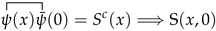 with being gauge-noninvariant Green function, see Eqn. (A.23). Using the relation which is similar to Eqn. (A.23), we can obtain that
After the factorization procedure, the matrix combination refers to the so-called hard part, while the non-perturbative hadron matrix element involves the gauge-invariant string operator defined as
with being gauge-noninvariant Green function, see Eqn. (A.23). Using the relation which is similar to Eqn. (A.23), we can obtain that
After the factorization procedure, the matrix combination refers to the so-called hard part, while the non-perturbative hadron matrix element involves the gauge-invariant string operator defined as
Appendix B. Local and Nonlocal Gauge Transform Convention
Before going further, it is important to remind the convention system regarding the gauge transformations which match the corresponding Wilson path functional (see [55] for more details). In what follows, for the sake of shortness, we say simply the Wilson line independently on the form of a path unless it leads to misunderstanding. For the non-Abelian gauge theory, let us now assume that the fermion and gauge fields are transformed as
where with being the generators of corresponding representations. With the local transformations fixed as in Eqns. (B.30) and (B.31), we can readily see that the covariant derivative and the gauge-invariant fermion string operator take the following forms:
with the Wilson line defined as
where stands for a path connecting the starting and destination x points in the Minkowski space.
Inserting the point in the Wilson line of the gauge-invariant string operator, see Eqn. (B.32), we get that
Eqn. (B.34) hints that the path-dependent non-local gauge transformation of fermions can be introduced in the form of
where is nothing but the Mandelstam gauge-invariant fermion field , modulo the global gauge transforms [54,74]. This transformation leads, in turn, to (cf. Eqn. (B.31))
Therefore, we have the following correspondence between local and non-local gauge transformation
which is extremely important for the further discussions because the wrong correspondence results in the substantially wrong conclusions (see for example [75]).
Appendix C. Gauge and Residual Gauge Symmetries
In this Appendix, we remind some subtleties related to the residual gauge transformations in different gauge theories.
Classical U(1)-Gauge Theory (Abelian Theory)
The -gauge theory where the gauge transformation
defines an orbit on the -group. In the Abelian case, the strength tensor is gauge-invariant and, therefore, only the longitudinal (unphysical) components of field, , can be gauge-transformed. Indeed, in the classical gauge theory for both and , the solution of the Maxwell equation in vacuum, , reads (modulo the complex conjugated terms), (see, e.g., [76])
where stands for the corresponding integration measure with an appropriate normalization, and . With this expression, we can easily derive the gauge transformations in p-space (= the momentum representation)
where the imaginary factor i is absorbed in the definition of . In what follows summation over and dimensionful normalizations are not shown explicitly unless it leads to misunderstanding.
Since , we conclude that
or, equivalently,
Moreover, it is easy to demonstrate that
where is a scalar function which is related to via the Fourier transformation, , and with for . Notice that if , the Maxwell equation takes the simplest form, , in the p-space and, therefore, or, in other words, .
As well-known, to fix the certain representative on the group orbit we have to impose a gauge condition on the gauge-transformed fields in order to find a solution with respect to the gauge parameter . Here, we do not discuss the appearance of Gribov’s ambiguity.
The Lorentz gauge. As the first example, we consider the Lorentz (covariant) condition which states
In p-space, the condition (C.44) takes the following form:
which gives us the relation for the case of . Notice that if , then the functions and in the combination are free functions and they are independent of each other.
However, the gauge condition (C.44) (or (C.45)) can not fix the orbit representative uniquely. Indeed, there is still the so-called residual gauge freedom defined by . For the Lorentz condition, two simultaneous conditions:
lead to
where the gauge function (parameter) defines the residual gauge freedom. That is, the residual gauge transformation with the function keeps the gauge condition, , gauge-invariant. Hence, the gauge freedom fixing means that one fixes all gauge freedom including the residual gauge. In other words, if there is no residual gauge transformation, the given gauge condition fixes the gauge freedom completely and we deal with one representative on a gauge orbit.
Let us consider the second gauge condition in Eqn. (C.46). In p-space, it leads to the following possibilities ( by definiton)
Hence, we can see that the gauge condition (C.46) cannot eliminate the unphysical field for the case of . Working with the equation (C.47), in the same manner, we conclude that the gauge function is not fixed and generates the residual gauge transformation provided .
It is instructive to consider the condition (C.47) in the coordinate representation (x-space). Solutions (C.47) can be easily found and represented, for instance, the following form:
Notice that the scalar function in Eqn. (C.43) which obeys the second condition in Eqn. (C.46), i.e. , has formally the same form as (C.49).
For , the scalar gauge function gives also the longitudinal (unphysical) field , see (C.45). Therefore, the first two solutions of (C.49) are irrelevant for our study. In order to get matched with the corresponding condition (C.48) in the momentum representation, we have to put be equal to zero, . However, for the case of , as above-mentioned, the functions and are independent and arbitrary due to the different free constant pre-factors in the plane wave solution.
We can also consider the Lorentz gauge condition (C.44) as an inhomogeneous differential equation with respect to , i.e.
where . Solving (C.50), we obtain that
where the Green function is defined as
with the suitable regularization of operator stemmed from the corresponding boundary conditions, see [67].
The Coulomb gauge. Using the condition to amplify the Lorentz condition (C.44), we can get the Coulomb gauge condition which reads
In p-space, the condition (C.53) is transformed to (recall that by construction)
Again, let us study the corresponding residual gauge freedom:
For the sake of simplicity, we dwell on the case of which leads to . With this, instead of (C.54), it is enough to stop on the equation
Hence, the only solution of (C.56) is which means that there is no any residual freedom at all.
Therefore, in the Coulomb gauge there are no the longitudinal field components and we deal with the physical gauge field only.
The Hamilton and axial gauges. In the similar manner, we can study the residual gauge symmetries in the Hamilton () and axial () gauges. The residual gauge transformations are given by the corresponding free (unfixed) gauge function provided or .
Classical SU(3)-Gauge Theory (Non-Abelian Theory)
The next subject of our discussion is a non-Abelian gauge theory with gauge group. In this case case, the gauge transformation is given by
which gives in the infinitesimal form
where . The decomposition of field components in the longitudinal and transverse components is similar to the Abelian case, see above. In contrast to the gauge group, the strength tensor is gauge-covariant. It means that all field components may change under gauge transformations.
The Lorentz gauge. We again begin with the Lorentz gauge condition:
As above-mentioned, the gauge condition is invariant under the residual gauge transformation:
or, equivalently,
where .
In p-space, the condition (C.61) takes the form of
If and, therefore, , then the gauge function cannot be fixed and generates the residual gauge transformation.
The Hamilton gauge. The similar situation occurs in the Hamilton gauge, . The residual transformation is induced by the gauge function which obeys
Hence, the solution of this equation is rather trivial: -function is the time-independent function, .
In the momentum representation, the condition (C.63) gives us the equation
which has a solution as
Therefore, we find in the coordinate representation
which coincides with the results of the preceding paragraph.
The axial gauge. Working in the axial gauge, , in the similar manner we are able to find the gauge function that is responsible for the residual gauge symmetry. We impose the condition
or, in the equivalent form,
The solution of this trivial differential equation is the -independent function which has the following form in p-space (cf. (C.64) and (C.65)):
where is an arbitrary gauge function related to the residual symmetry.
It is instructive to focus on the finite gauge transformations and corresponding gauge condition, namely
The solution of this equation can easy be found, it reads
where, generally speaking, is an arbitrary constant. We stress that the solution is valid for . At the same time, this function can be multiplied by an arbitrary -independent gauge function to produce another solution of equation (C.70), i.e.
where . Indeed, one can demonstrate that .
To study the residual symmetry, we have to demand that for any x. Therefore, from (C.72), we obtain that the function
generates the residual transformation we are interested in.
Let us now return to the gauge function presented by (C.69). The case of (which provides us the residual symmetry) leads to the so-called spurious singularity in the gluon propagator in the axial gauge, see the next subsection. If we adopt a procedure to regularize this singularity with the help of some well-defined procedure, , then the existence condition for the residual symmetry, see (C.68), has to be given by (in the momentum representation)
Hence, the only possibility to satisfy this equation is to demand that which means that we fix the remaining residual symmetry. Thus, we conclude that the spurious singularity is fixed if and only if we do not have the residual gauge symmetry. On the other hand, we may say that the residual gauge fixing is enough for the elimination of spurious singularity.
Spurious Singularity of Gluon Propagator
Let us return to the issue of the spurious singularity which appears in the gluon propagator in the axial gauge .
The generating functional for gluons (gluonodynamics) in the most general gauge
where involves the infinite gauge group volume, , and we use
Instead of solving the gauge condition with respect to the group function within the generalized Hamilton formalism, we separate out the infinite group volume, , in the generating functional (the Faddeev-Popov approach).
The next trick is related to the exponentiation of . We introduce the generalized gauge condition as with . The generalizing functional must be independent on C. Therefore, to get the C-independent functional we have to integrate out over this parameter C. Using the integration measure defined as
we have
In (C.78), the effective action with the gauge-fixing term,
is now not gauge-invariant anymore. As a result of this trick, we don’t need to solve the gauge condition with respect to the gauge function.
Let the gauge condition be with . In this case, the determinant is independent on A and, therefore, we are able to include this determinant in the normalization of functional. Thus, the effective Lagrangian reads
This Lagrangian yields the effective action which can be written as
where
In p-space, the operator has an inverse operator which, in the limit of , is given by
As we have demonstrated in the preceding subsection, when we fix/regularize the spurious singularity it means that we fix the residual gauge symmetry defined by the gauge function and vise versa.
We also remind that it is not possible to fix the residual gauge simply by means of adding of
in Eqn. (C.80). In this case, the inverse kinematical operator (see, Eqn. (C.83)) does not exist due to the fact that the free (without the coefficients) tensors and present in the corresponding equation to determine the coefficients. Indeed, introducing the Lorentz parametrization (where the coefficients have to be determined)
where
the contraction equation on the coefficients (or, in other words, the Green function equation)
involves the tensors and which stay without coefficients. It means that the inverse operator cannot be derived.
References
- L. D. Faddeev and A. A. Slavnov, Front. Phys. 50, 1-232 (1980).
- I. V. Anikin and A. S. Zhevlakov, “Spin and orbital angular momentum separation: Theorem on decomposition” [arXiv:2105.02719 [hep-ph]].
- R. Angeles-Martinez et al., Acta Phys. Polon. B 46 (2015) no.12, 2501 [arXiv:1507.05267 [hep-ph]].
- D. Boer et al., arXiv:1108.1713 [nucl-th].
- Z. B. Kang, J. W. Qiu, W. Vogelsang and F. Yuan, Phys. Rev. D 83, 094001 (2011).
- D. Boer, Phys. Lett. B 702, 242 (2011).
- D. Boer, P. J. Mulders and F. Pijlman, Nucl. Phys. B 667, 201 (2003).
- B. Pire and J. P. Ralston, Phys. Rev. D 28, 260 (1983).
- R. D. Carlitz and R. S. Willey, Phys. Rev. D 45, 2323 (1992).
- A. Brandenburg, D. Mueller and O. V. Teryaev, Phys. Rev. D 53, 6180 (1996).
- A. P. Bakulev, N. G. Stefanis and O. V. Teryaev, Phys. Rev. D 76, 074032 (2007).
- A. V. Radyushkin, Phys. Rev. D 80, 094009 (2009).
- M. V. Polyakov, JETP Lett. 90, 228 (2009).
- S. V. Mikhailov and N. G. Stefanis, Mod. Phys. Lett. A 24, 2858 (2009).
- D. Boer, P. J. Mulders and O. V. Teryaev, Phys. Rev. D 57, 3057 (1998).
- I. V. Anikin and O. V. Teryaev, Phys. Lett. B 690, 519 (2010).
- I. V. Anikin and O. V. Teryaev, Eur. Phys. J. C 75, no. 5, 184 (2015).
- A. V. Belitsky, X. Ji and F. Yuan, Nucl. Phys. B 656, 165 (2003).
- G. A. Chirilli, Y. V. Kovchegov and D. E. Wertepny, JHEP 1512, 138 (2015)bibitemSoper:1979fq D. E. Soper, Phys. Rev. Lett. 43 (1979) 1847.
- J. C. Collins and D. E. Soper, Nucl. Phys. B 194 (1982) 445.
- G. Leibbrandt, Rev. Mod. Phys. 59 (1987) 1067.
- A. A. Slavnov and S. A. Frolov, Theor. Math. Phys. 73 (1987) 1158 [Teor. Mat. Fiz. 73 (1987) 199].
- A. Bassetto, G. Nardelli and R. Soldati, “Yang-Mills theories in algebraic noncovariant gauges: Canonical quantization and renormalization,” Singapore, Singapore: World Scientific (1991) 227 p.
- A. Bassetto, M. Dalbosco, I. Lazzizzera and R. Soldati, Phys. Rev. D 31 (1985) 2012.
- J. C. Collins, D. E. Soper and G. F. Sterman, Adv. Ser. Direct. High Energy Phys. 5 (1989) 1,.
- S. V. Ivanov, Fiz. Elem. Chast. Atom. Yadra 21 (1990) 75.
- N. G. Stefanis, Nuovo Cim. A 83 (1984) 205.
- X. Ji, F. Yuan and Y. Zhao, Nature Rev. Phys. 3, 27 (2021).
- R. L. Jaffe and A. Manohar, Nucl. Phys. B 337, 509 (1990).
- X. D. Ji, Phys. Rev. Lett. 78, 610 (1997).
- X. S. Chen et al, Phys. Rev. Lett. 100, 232002 (2008).
- X. S. Chen et al, Phys. Rev. Lett. 103, 062001 (2009).
- X. Ji, Phys. Rev. Lett. 106, 259101 (2011).
- M. Wakamatsu, Int. J. Mod. Phys. A 29, 1430012 (2014).
- M. Wakamatsu, Eur. Phys. J. A 51, 52 (2015).
- M. Wakamatsu et al, Annals Phys. 392, 287 (2018).
- C. Lorce, Phys. Lett. B 719, 185 (2013).
- C. Lorcé, Phys. Rev. D 88, 044037 (2013).
- E. Leader and C. Lorcé, Phys. Rept. 541, 163 (2014).
- M. Wakamatsu, Phys. Rev. D 84, 037501 (2011).
- M. Wakamatsu, Phys. Rev. D 83, 014012 (2011).
- M. Wakamatsu, Phys. Rev. D 81, 114010 (2010).
- P. M. Zhang and D. G. Pak, Eur. Phys. J. A 48, 91 (2012).
- S. Bashinsky and R. L. Jaffe, Nucl. Phys. B 536, 303 (1998).
- A. V. Belitsky and A. V. Radyushkin, Phys. Rept. 418, 1 (2005).
- S. V. Ivanov, G. P. Korchemsky and A. V. Radyushkin, Yad. Fiz. 44, 230 (1986) [Sov. J. Nucl. Phys. 44, 145 (1986)].
- S. V. Ivanov and G. P. Korchemsky, Phys. Lett. B 154, 197 (1985).
- I. V. Anikin, “On the use of non-local gauges in QFT,” [arXiv:2105.09430 [hep-ph]].
- I. V. Anikin, D. Y. Ivanov, B. Pire, L. Szymanowski and S. Wallon, Nucl. Phys. B 828, 1 (2010).
- N. P. Konopleva and V. N. Popov, “Gauge Fields,” Translated from the Second Russian Edition and edited by N.M. Queen, Harwood Academic Publishers, (1981).
- V. I. Shevchenko and Y. A. Simonov, Phys. Lett. B 437, 146-152 (1998).
- M. B. Mensky, Theor. Math. Phys. 173, 1668 (2012).
- M. B. Mensky, “The Path Group: Measurements Fields Particles”, Nauka Moscow (1983).
- S. Mandelstam, Annals Phys. 19, 1 (1962).
- I. V. Anikin, I. O. Cherednikov and O. V. Teryaev, Phys. Rev. D 95, no. 3, 034032 (2017).
- I. V. Anikin, Symmetry 12, no.12, 1996 (2020).
- D. Boer and J. w. Qiu, Phys. Rev. D 65, 034008 (2002).
- N. Hammon, O. Teryaev and A. Schafer, Phys. Lett. B 390, 409 (1997).
- D. Boer, P. J. Mulders and O. V. Teryaev, Phys. Rev. D 57, 3057 (1998).
- Y. Hatta, Phys. Rev. D 84, 041701 (2011).
- L. Durand and E. Mendel, Phys. Lett. 85B, 241 (1979).
- V. P. Nair, “Elements of Geometric Quantization and Applications to Fields and Fluids” [arXiv:1606.06407 [hep-th]].
- V. Barone, A. Drago and P. G. Ratcliffe, Phys. Rept. 359, 1 (2002).
- A. V. Efremov and O. V. Teryaev, Phys. Lett. B 150, 383 (1985).
- I. V. Anikin and O. V. Teryaev, Phys. Part. Nucl. Lett. 6, 3 (2009).
- V. M. Braun, D. Y. Ivanov, A. Schafer and L. Szymanowski, Nucl. Phys. B 638, 111 (2002).
- N. N. Bogolyubov and D. V. Shirkov, “Introduction To The Theory Of Quantized Fields,” Intersci. Monogr. Phys. Astron. 3, 1 (1959).
- A. V. Efremov and A. V. Radyushkin, Theor. Math. Phys. 44, 774 (1981) [Teor. Mat. Fiz. 44, 327 (1980)].
- V. S. Vladimirov, “Generalized Functions in Mathematical Physics”, Mir Publishers (1979) 390 p.
- H. Weigert and U. W. Heinz, Z. Phys. C 56 , 145 (1992).
- D. J. Gross and S. B. Treiman, Phys. Rev. D 4, 1059 (1971).
- I. I. Balitsky and V. M. Braun, Nucl. Phys. B 311, 541 (1989).
- A. V. Radyushkin, Fiz. Elem. Chast. Atom. Yadra 14, 58 (1983).
- B. S. DeWitt, Phys. Rev. 125, 2189 (1962).
- C. Lorce, Phys. Rev. D 87, 034031 (2013).
- V. A. Rubakov, “Classical theory of gauge fields”, Princeton, USA: Univ. Pr. (2002) 444 p.
Figure 1.
The H-system with unresolved and resolved constrains. The left panel represents the system with the inner (gauge) symmetry; the right panel corresponds to the system with the fixed (preferable) site on the ball surface.
Figure 1.
The H-system with unresolved and resolved constrains. The left panel represents the system with the inner (gauge) symmetry; the right panel corresponds to the system with the fixed (preferable) site on the ball surface.
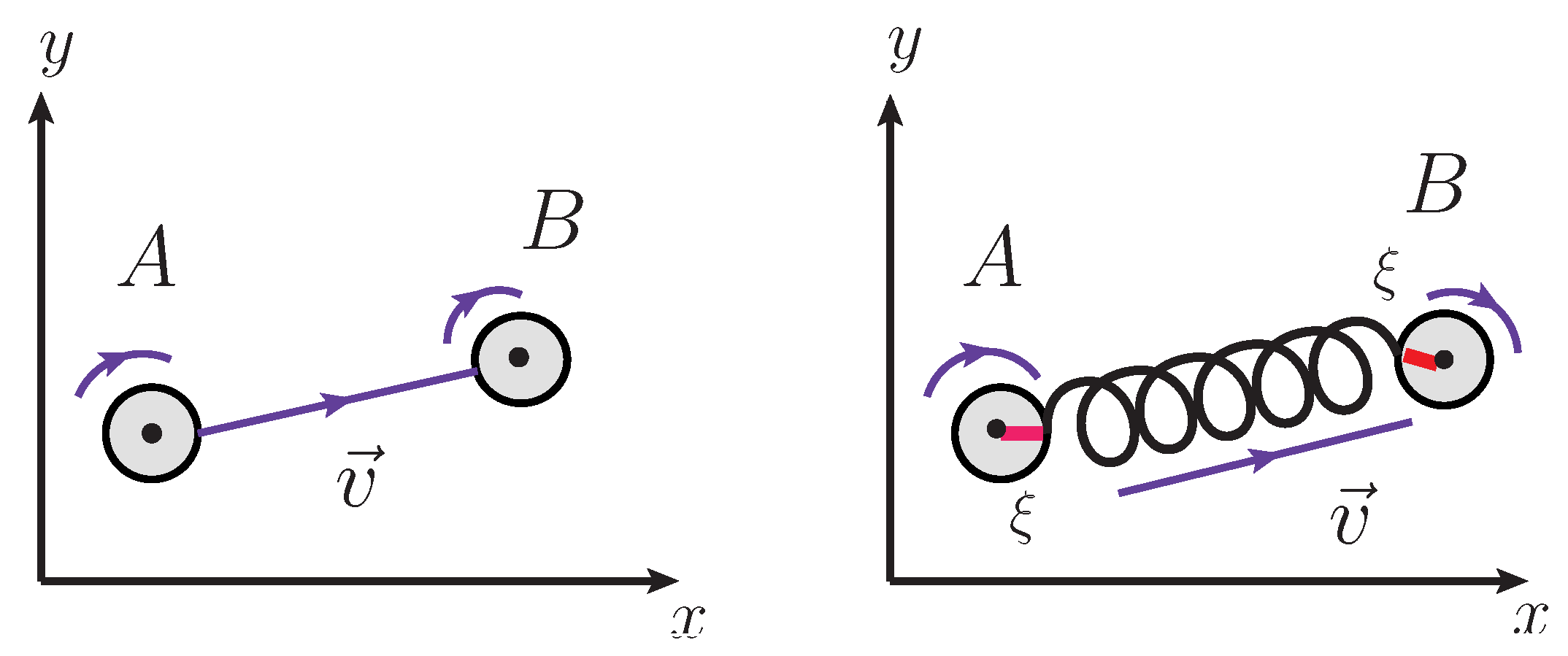
Figure 2.
The contour gauge: the plane of in the principle fiber bundle .
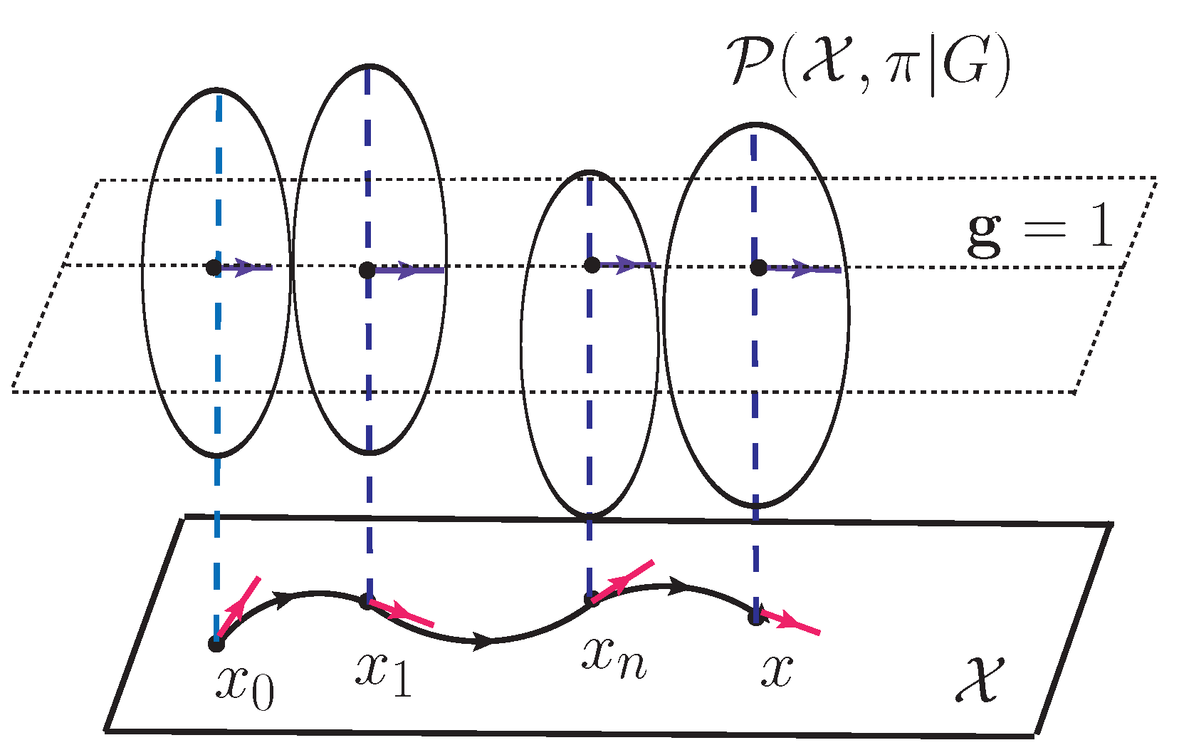
Figure 3.
The Feynman diagrams which contribute to the polarized Drell-Yan hadron tensor: the standard (the left panel) and non-standard diagrams (the right panel).
Figure 3.
The Feynman diagrams which contribute to the polarized Drell-Yan hadron tensor: the standard (the left panel) and non-standard diagrams (the right panel).
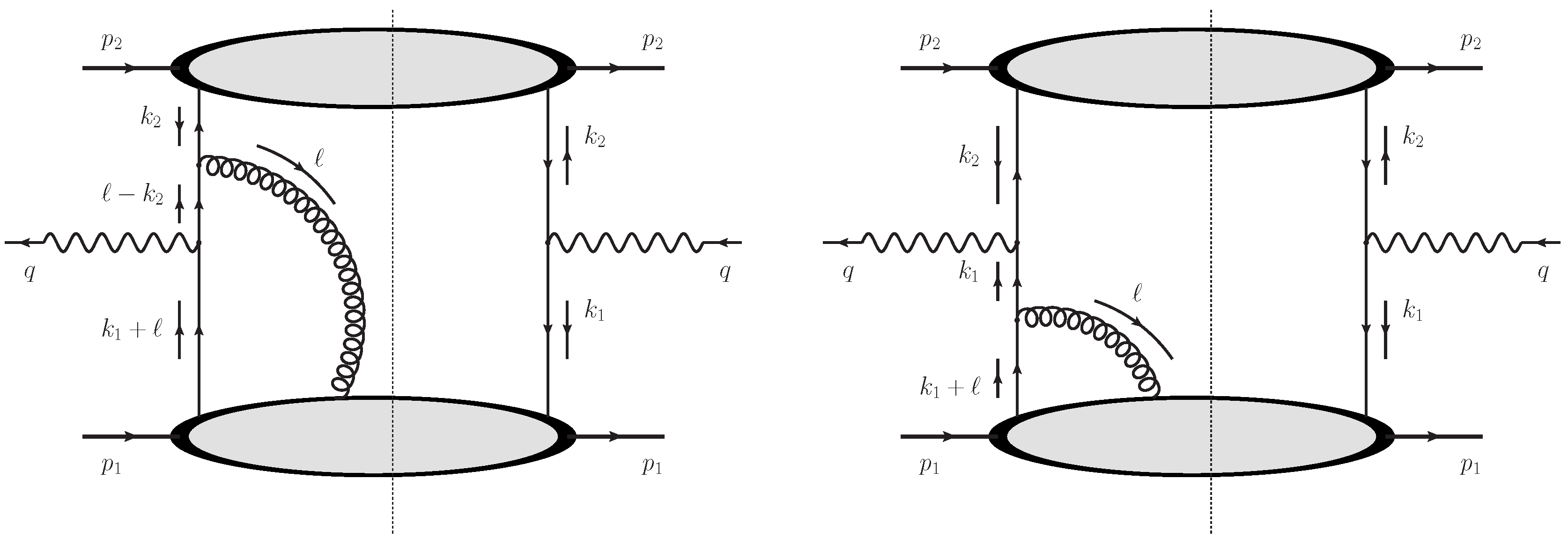
Figure 4.
The longitudinal Wilson lines related to the standard (red lines, the exponentials with ) and non-standard (blue lines, the exponentials with ) Drell-Yan hadron tensor. The circles single out the interception points which the continuity conditions are defined for.
Figure 4.
The longitudinal Wilson lines related to the standard (red lines, the exponentials with ) and non-standard (blue lines, the exponentials with ) Drell-Yan hadron tensor. The circles single out the interception points which the continuity conditions are defined for.
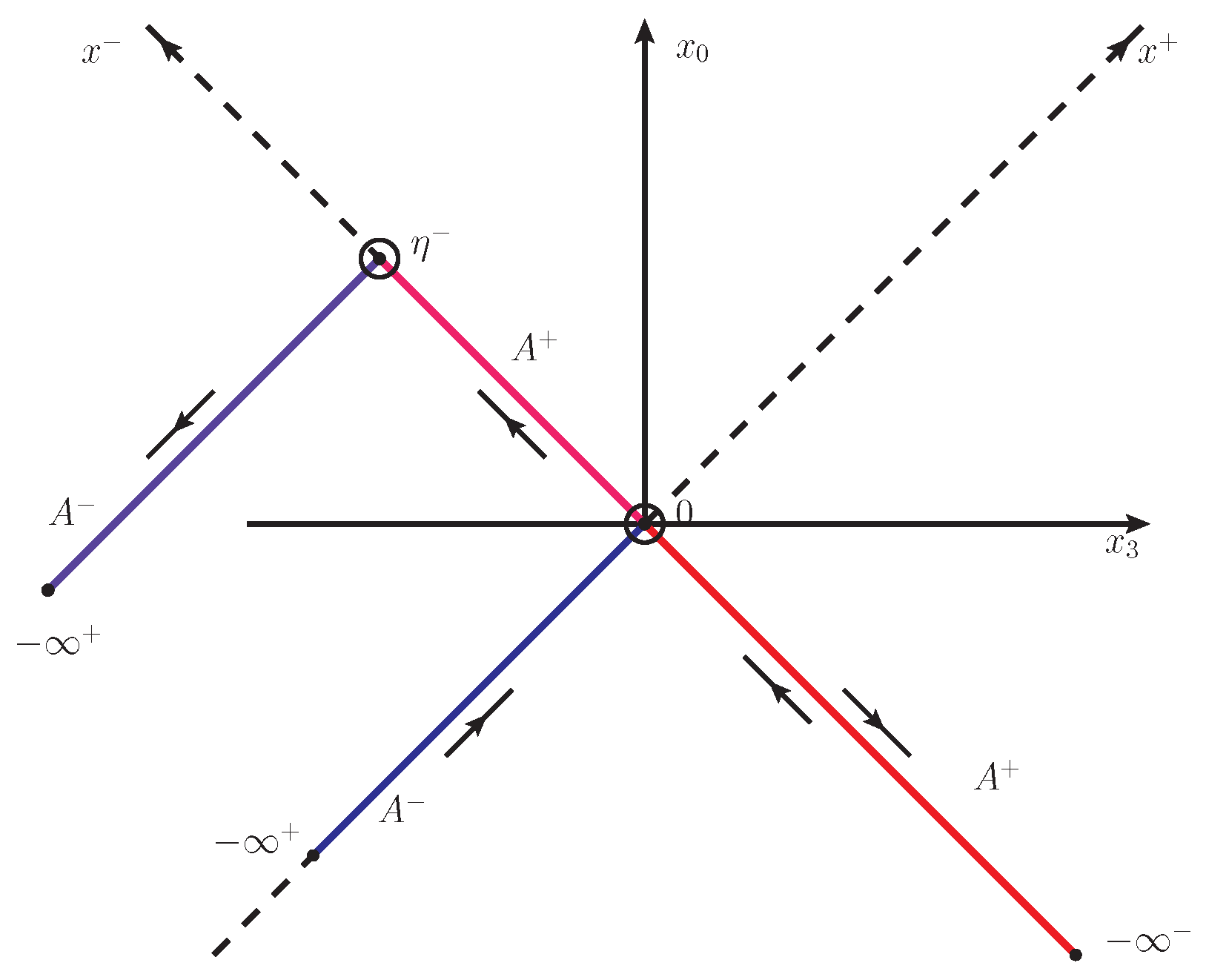
Figure 5.
The holonomy: with denote the corresponding horizontal vectors defined on the given fiber of .
Figure 5.
The holonomy: with denote the corresponding horizontal vectors defined on the given fiber of .
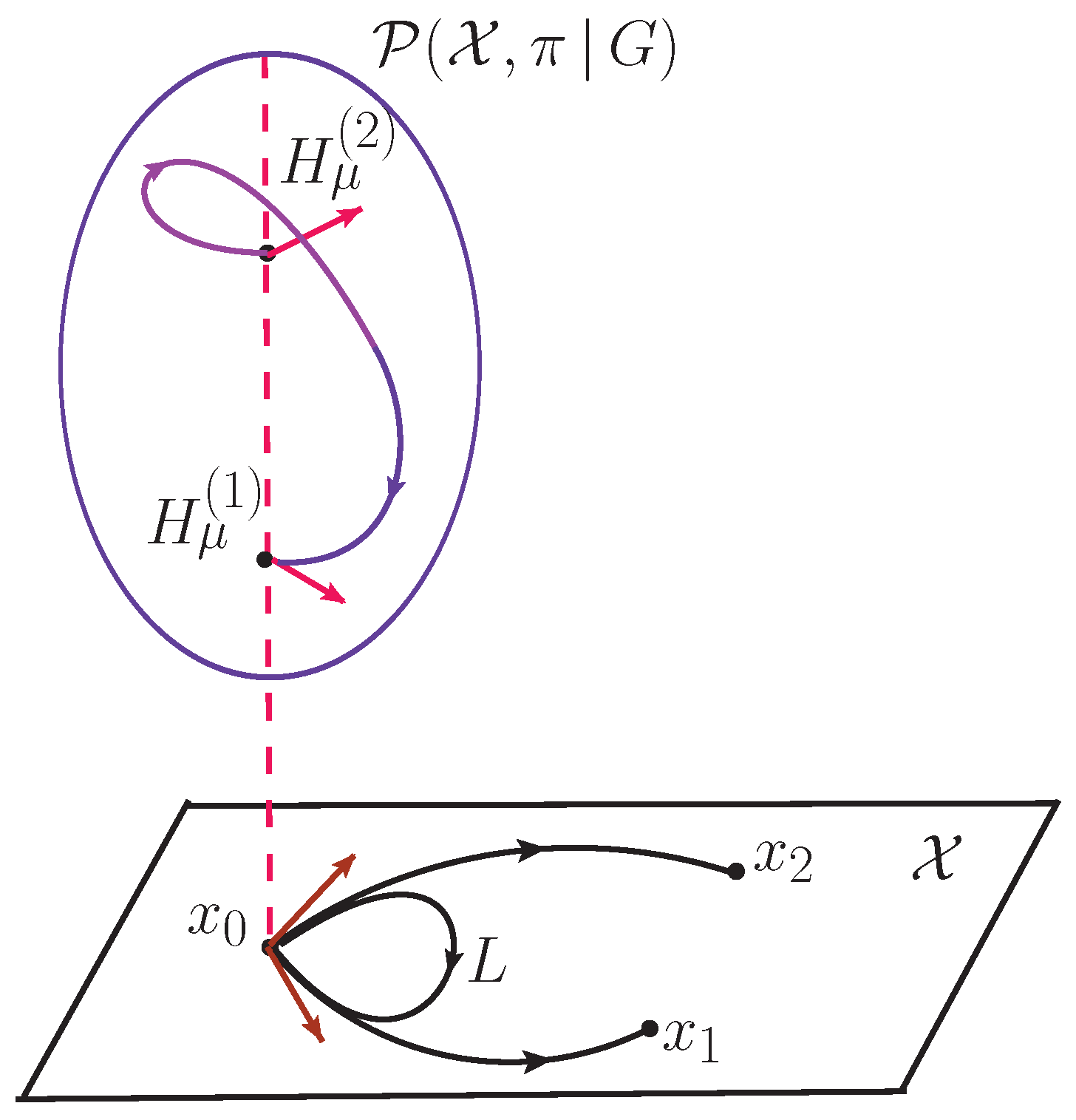
Figure 6.
The angle independence of the starting point O: and ; where with .
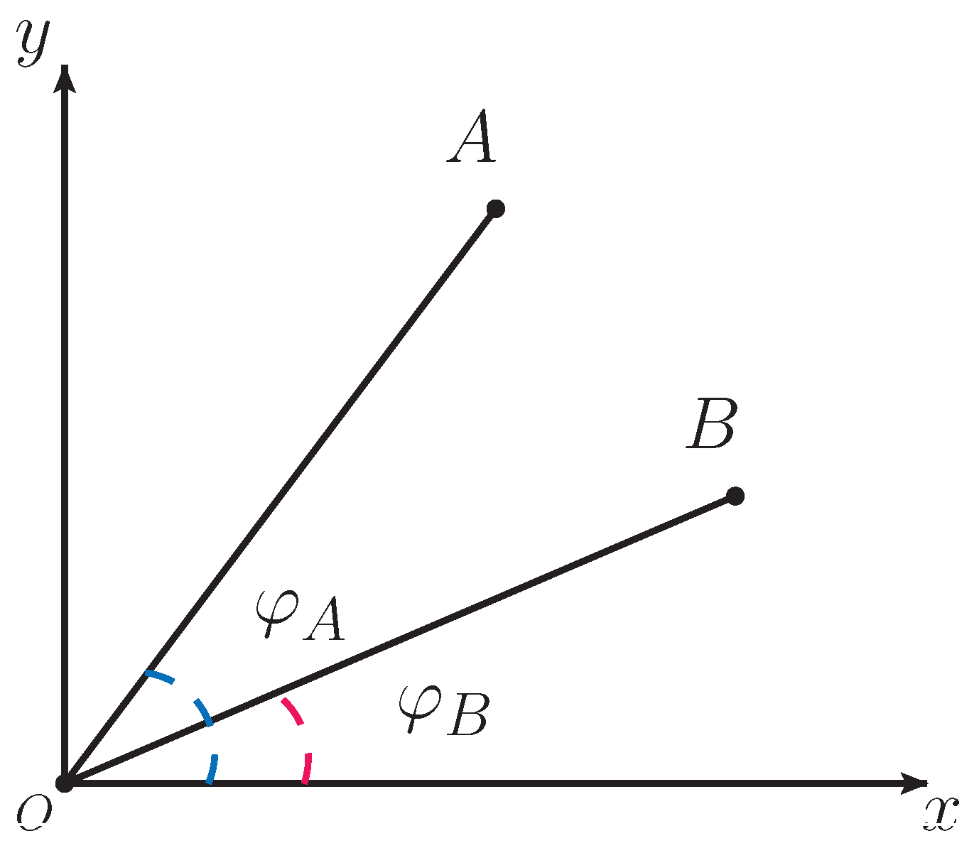
Disclaimer/Publisher’s Note: The statements, opinions and data contained in all publications are solely those of the individual author(s) and contributor(s) and not of MDPI and/or the editor(s). MDPI and/or the editor(s) disclaim responsibility for any injury to people or property resulting from any ideas, methods, instructions or products referred to in the content. |
© 2023 by the authors. Licensee MDPI, Basel, Switzerland. This article is an open access article distributed under the terms and conditions of the Creative Commons Attribution (CC BY) license (http://creativecommons.org/licenses/by/4.0/).
Copyright: This open access article is published under a Creative Commons CC BY 4.0 license, which permit the free download, distribution, and reuse, provided that the author and preprint are cited in any reuse.


