

Submitted:
04 August 2023
Posted:
07 August 2023
You are already at the latest version
Abstract
In this study, reinforcement learning (RL) was used in factory simulation to optimize storage devices for use in Industry 4.0 and digital twins. First, we defined an RL environment, modeled it, and validated its ability to simulate a real physical system. Subsequently, we introduced a method to calculate reward signals and apply them to the environment to ensure the alignment of the behavior of the RL agent with the task objective. The stocker simulation model was used to validate the effectiveness of RL. The model is a storage device that simulates logistics in a manufacturing production area. The results revealed that RL is a useful tool for automating and optimizing complex logistics systems and increase the applicability of RL in logistics. We proposed a novel method for creating an agent through learning using the proximal policy optimization algorithm, and the agent was optimized by configuring various learning options. The application of reinforcement learning resulted in an effectiveness of 30% to 100%, and methods can be expanded to other fields.
Keywords:
conceptualization
; methodology
; job allocation
; reinforcement learning
; stocker
; digital twin
; simulation
; Industry 4.0
1. Introduction
Factory automation and logistics optimization are crucial for enhancing the efficiency and productivity of factories. Logistics automation is a dynamic area of research [1]. Advanced technologies such as intelligent stockers have been introduced to automate logistics in factories and improve the efficiency of movement and storage of goods in factories. Optimizing the route selection, goods placement, storage volume, and work order of the robot is crucial for effectively using these technologies[2]. Reinforcement learning (RL) is an effective approach for solving complex problems by learning through trial and error. In particular, using RL in factory simulations is highly promising in optimizing logistics automation [3].
Considering industry trends that focus on streamlining production processes for new products and automating logistics is critical. These trends indicate that logistics systems in factories are becoming increasingly organized, and automation technologies are advancing [4]. Logistics automation is a critical component of factory operations, and an efficient logistics system considerably affects the productivity and competitiveness of a factory. Studies have focused on optimizing logistics automation systems using RL based on artificial intelligence [5]. RL algorithms can improve and optimize logistics automation processes in factory simulations. However, automating logistics in factories can be expensive. The optimization of suitable requirements, the implementation of real-time autonomous judgment and autonomous driving technologies, and the use of RL, a sequential action decision technique, are crucial methodologies for addressing these concerns. However, challenges, such as insufficient training data, high cost of trial and error, and potential risk of accidents resulting from trial and error, remain [6]. These systems can increase the efficiency of the logistics system of a factory. However, many factories are yet to use them properly [7].
This methodology for optimizing storage in logistics automation combines factory simulation with artificial intelligence (AI) technology. The method predicts various problems that may occur on the production line to improve efficiency[8]. An RL model simulates various scenarios and continuously adjusts to determine the optimal solution and optimize storage. Thus, analyses of the data required for logistics operations can be performed to determine the optimal response. The RL model analyzes the quantity, type, and quality of goods in the production line. Based on this result, data related to the operational patterns of logistics automation robots are collected and continuously adjusted. RL models can be used to determine optimized routes that efficiently use various resources required for logistics tasks and reduce work time and prevent problems from occurring on the production line [9].
Complex processes from real factory operations can be modeled in a digital environment by combining factory simulation with RL to improve work efficiency and logistics processes within the factory [10]. This approach can improve overall factory productivity. Moreover, optimizing logistics automation can save labor, time, and cut down expenses. In particular, in logistics automation, we proposed to optimize the total capacity of the stocker, a storage device, which is expected to show savings of approximately 30% or more and increase the overall efficiency of the logistics system.
The contributions of this paper are as follows: Optimizing logistics automation is critical to increasing productivity and getting products to market. Reinforcement learning (RL) algorithms can improve and optimize the logistics automation process in factory simulations because they use trial and error until the optimal solution for logistics automation is determined. It can be used as a guideline for developing effective simulation solutions to improve logistics efficiency.
The remainder of this paper is organized as follows. Section 2 of this paper discusses factory simulation, RL, and storage devices, and presents the proposed optimization technique. Section 3 describes the proposed model for optimizing storage using RL. We describe the techniques and roles of RL, virtual factory processes, and AI applications in factory simulation. Section 4 describes the modeling process for simulating a factory, including implementation, learning, result calculation, and hypothesis validation using optimization AI. Finally, Section 5 summarizes the optimization techniques, implementation, and test results presented in this paper, and discusses potential avenues for future research.
2. Related work
2.1. Factory Simulation
Factory simulation is a crucial field that is used to model and optimize manufacturing and operational processes.
Figure 1 Simulation models play a crucial role in manufacturing planning and control because they allow companies to assess and enhance their operational strategies. Simulation models provide a digital representation of a manufacturing system, which enables decision makers to experiment with various scenarios, test hypotheses, and determine the optimal course of action. Optimization-based simulation combines simulation models with optimization techniques to determine the optimal solution for manufacturing planning and control problems.
Models incorporate mathematical optimization algorithms, such as linear programming or genetic algorithms, to optimize performance metrics such as production throughput, inventory levels, and Make-Pan. Models can be used to resolve complex scheduling, routing, or resource allocation problems [11]. A virtual model of a factory was created, and its operations were simulated to analyze and optimize its capacity, efficiency, and performance. Manufacturers can use factory simulation to test various scenarios and make informed decisions regarding capacity planning, production scheduling, and resource allocation. Manufacturers can also identify bottlenecks, optimize workflows, and improve overall productivity [12]. Discrete-event simulation can assist manufacturers identify bottlenecks, optimize workflows, and enhance productivity. By simulating the performance of manufacturing systems, manufacturers can identify areas for improvement and optimize operations before implementing them in the real-world [13]. Agent-based modeling and simulation can be used to predict the effect of changes in a system, such as alterations in demand, production processes, or market conditions. Manufacturers and businesses can proactively adjust their operations to reduce the risk of downtime, delays, and other disruptions, model and analyze complex systems, and optimize their operations using this technology [14].
2.2. RL
RL is machine learning method that involves rewarding a behavior in a specific environment to determine its effectiveness and subsequently training to maximize the reward through repetition.
Figure 2 Reinforcement learning consists of two components, namely the environment and the agent. RL is defined by the Markov Decision Process (MDP), which is the assumption that the state at any point in time is only affected by the state immediately prior to that point in time [15].
Markov Assumption : P(s | s), s,…,s) = P(s |s)
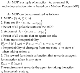
Unlike MP, MDP adds a decision-making process, so the agent should determine its behavior for each state.
1. The agent must decide what action a to take in any state s, which is called a policy.
A policy is defined as follows:
2. RL is a learning policy that involves trial and error to maximize the reward.The goodness or badness of an action is determined by the sum of the rewards, which is defined as the return value G.
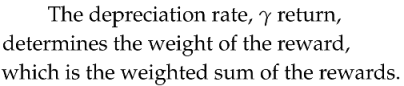
The depreciation rate is typically expressed as . The value can be set to a value between 0 and 1, with a value closer to 1 which reveals more weight is placed on future rewards. In RL maximizing reward denotes maximizing return not just one reward [16].
In RL an agent receives a reward for performing a specific action in a particular state and learns to optimize this reward. Through trial and error, the agent selects actions that maximize its reward, and this iterative process optimizes its reward. Unlike supervised learning, RL does not require any pre-prepared data and can be trained with small amounts of data. To address challenges, such as accurately detecting the position and orientation of objects, robots encounter during pick-and-place tasks, deep learning techniques are used to predict their location and orientation. To accomplish this task, the robot uses its camera to identify objects and a deep learning model is used to anticipate their position and alignment. To address the problem of a robot inaccurately picking objects during a pick-and-place task, we used RL to train the robot to accurately grasp objects. By using a RL algorithm, the robot receives rewards for accurately picking up objects and is penalized for any incorrect pickups. Studies have revealed that this method exhibits high accuracy and stability when robots perform pick-and-place tasks [17]. Deep Q-learning (DQL) enables a robot to collect goods in a warehouse and automatically fulfill orders. The robot receives a list of orders, collects necessary goods, and processes them using DQL algorithms to determine the most efficient path. The optimal behavior is selected by approximating the Q-function using a deep learning model. The robot determines the most efficient route for collecting goods, which reduces the processing time [18].
2.3. Storage Devices
A device that stores products and materials on a manufacturing floor is called a stocker. Stockers automate the storage and movement of raw materials and finished goods, both in and out of a facility. Stockers operate in conjunction with a logistics automation system to streamline the supply chain process and can perform additional functions, such as splitting, merging, and flipping, as required. These functions allow the stocker to efficiently manage logistics throughout the manufacturing process.
Figure 3 initially, stockers were managed by people, and logistics were transported manually. To optimize the number and use of stockers, several factors, including space utilization, demand forecasting, inventory turnover, and operational efficiency, should be considered. Depending on the type of product and the requirements of the site, either the first-in, first-out (FIFO) or last-in, first-out (LIFO) method is applied [19]. FIFO reduces the risk of goods becoming obsolete by using older inventory first. By contrast, LIFO may be appropriate for products with a longer shelf life [20].
Figure 4 Stocker’s automation has been used for intelligent storage and management of products and materials to improve the efficiency and accuracy of storage operations in factories.
An overview of the various types of archivers is presented here. Storage devices are selectively used based on the production environment.
Figure 5 Single and double-deep racks are both types of selective pallet racks, which are among the most popular options for inventory storage in use today. Single-deep assemblies are installed back to back to create aisle ways for forklifts to access the palletized inventory. Each inventory pallet is easily accessible from the aisle using standard material handling equipment. Figure 6 Drive-in and Drive-thru storage systems are free-standing and self-supporting racks that enable vehicles to drive-in and access the stored products. Drive-in racks exhibit a higher storage capacity within the same cubic space compared to other conventional racking styles, and reduce the cost per square foot of pallets. Drive-thru racks are similar to drive-in racks, with the exception that vehicles can access the rack from either side, rendering them versatile and efficient. Figure 7 Live storage system for picking, also called carton flow rack, permits high-density storage of cartons and light products, which results in savings in the space and improved stock turnover control. In this picking system, we ensure perfect product rotation by following the first-in, first-out (FIFO) system. Additionally, we avoid interference by differentiating the loading and unloading areas.
Figure 8 Pallet flows racking, which is also known as pallet live storage, gravity racking, and a FIFO racking system. This storage solution is designed for high-density storage of pallets, and it allows loads to move by gravity. Palletized loads are inserted at the highest point of the channel and move by gravity to the opposite end, where they can be easily removed. A flow rack system does not have intermediate aisles, which enhances its storage capacity. Figure 9 Push-back racking system, which is a pallet storage method that enables storage of pallets from two to six deep on each side of an aisle. This method provides higher storage density than other forms of racking. A push-back rack system consists of a set of inclined rails and a series of nesting carts that run on these rails. Figure 10 Mobile Rack is a shelving system on wheels designed to increase space efficiency in warehouses and logistics operations. Unlike typical fixed racks, the mobile rack sits on movable tracks and can be easily relocated as desired. This mobility enables the optimal utilization of the warehouse space, which increases its efficiency.
Figure 11 Rack master can be a valuable asset in warehousing and logistics systems, particularly when the space is limited inside the warehouse. Because the rack master is customized to satisfy the specific needs of each customer, it can provide numerous functions that cater to those needs. The rack master is widely used in warehouse and logistics systems, rendering it an essential component in this field.
3. RL Based Storage Optimization
3.1. Overall Architecture
Factory simulation involves using a computer-based virtual environment to model and simulate the operations of an actual factory.
Figure 12 Simulation optimizes factory operations and enhances the efficiency of production lines. Furthermore, the components of a factory, including production lines, equipment, workers, and materials, can be virtually arranged to replicate various operational scenarios and evaluate the outcomes [21]. This simulation improves the efficiency of a real factory’s operations, optimize production planning, and enhance overall productivity.
Figure 13 Factory simulation and RL can be combined to model the complex processes of real-world factory operations in a digital environment for experimentation and analysis [22]. RL algorithms are used as agents in the factory simulation to learn logistics processes. These algorithms enable them to optimize the logistics processes and automation systems of the factory. By implementing this approach, the complexity of real-world factory operations can be effectively managed to improve the efficiency of logistics processes [23].
3.2. Virtual Factory Processes
Virtual factories are used in situations in which a physical factory has not yet been constructed, or when an existing factory is to be analyzed or enhanced, but performing such analysis in a real-world setting is challenging. A factory can be established in this scenario. A virtual space accords various spaces for analyses and evaluation [24]. Factory simulation utilizes three-dimensional (3D) simulation software to analyze the logistics flow of the factory, the equipment utilization rate, and potential losses such as line of balance and bottleneck issues. The optimal factory structure when introducing new equipment or transportation devices can also be simulated [25].
Figure 14 Virtual factory process involves simulating and mimicking real-life factory operations. To improve the efficiency, productivity, and resource utilization of factory operations, numerous processes are undertaken. These processes include design and modeling, data collection, simulation execution, performance evaluation and optimization, decision-making, strategy formulation, and system integration. This resource provides a comprehensive understanding of factory operations and insights into the construction and functioning of an actual factory [26].
Figure 15 Through the systematic use of virtual verification, factory simulation helps manufacturers predict and address various problems that may emerge during the production process. By modeling the behavior of systems in advance, strategies can be developed for production and operations that increase efficiency, safety, and profitability. Additionally, analyzing the expected results of adjusting and changing various variables can improve these outcomes.
3.3. Applying AI technology
Effectively optimizing complex simulations by exploring optimal design directions using AI.
The accuracy of the data enables clear visibility and precise location and dimensioning during the transition from 2D to 3D. Efficient resource utilization maximizes production by optimizing resource input. Figure 16 AI algorithms are used in production optimization [27] to efficiently manage the logistics and resources of a factory, optimize areas of logistics automation. When applying the proximal policy optimization (PPO) algorithm to a factory simulation, PPO functions as a RL agent that learns optimal policies by interacting with the simulated environment. This phenomenon can be used in factory simulations to help agents make decisions about factory operations. For instance, the PPO algorithm can be used to solve decision-making problems, including but not limited to storage management, production planning, and resource allocation. This phenomenon can considerably improve the efficiency of factory operations [28].
The subjective symptoms are ignored when an objective is initially opened, but they are considered when the objective worsens [29].
The loss function for the PPO algorithm is expressed as follows:
The motivation of the objective function is as follows: the first term in the “Min” function represents the objective function of trust region policy optimization. The second term modifies the surrogate objective by limiting the probability ratio, which removes the motivation for RTs to move beyond []. The ultimate objective is to establish a lower limit for the unclipped objective by selecting the smaller value between the clipped objective and the unclipped objective. In this approach, only changes in the likelihood ratio are considered.
4. Simulation and Results
4.1. Simulation Environment
The simulation environment that is validated in this study is a component of a production line that produces battery management systems. Figure 17 displays the production system design in which we compare the performance indicators of conventional (FIFO) and RL approaches for task distribution based on the model to optimize storage capacity. The production system was modeled using FlexSim simulation software for validation [30]. To implement RL, we used the PPO algorithm from the Stable-Baseline3 library [31], which is known for its effectiveness in solving numerous problems. PPO is a policy gradient method that directly optimizes an agent’s policy function in an RL setting. The objective of the agent is to acquire a policy that maximizes the total reward that it obtains over certain time [32].
4.2. Performance Metrics
Items are categorized into four types, namely 1, 2, 3, and 4. Each type has an equal probability of occurring, with a 1/4 chance of a particular item being type i (where i = 1, 2, 3, or 4). Additionally, the type of a specific work piece is not influenced by the types of its preceding or succeeding work pieces. Both Board Assemblies 1–2 and Router1–3 can process all types of jobs, but the individual processing time for each type varies, as presented in Table 1. Router1. If the type of a particular job differs from the type of the previous job, 3 has a setup time of 20s.
- -. Average Production per Type
- -. Average Stocker Load
- -. Average Buffer Latency per Type
Table 1 Set the four types, Board Assy. and router’s process time.
- - Router setup time: 20 s
- - Item generation: Type 1–4 with uniform probability
- - Run time: 10 days (warm-up time: 3 days)
- - RL algorithm:
- : PPO algorithm
- - Time step (number of training times): 10,000 times
- - Reward definition:
Router average Process Time)/(Item Sink1 entry time - Item Stocker exit time) The formula for router average Process Time)/(Item Sink1 entry time - Item Stocker exit time). To implement the model shown in Figure 17. which can be used to direct items entering the stocker to the optimal object among Router1-3, the reinforcement learning components are as follows: State: St = [Router1 Type-1, Router2 Type-1, Router3 Type-1] In the state expression, Router1 through Router3 Type-t-1 refers to the type number of the (t-1) job processed by Router1 through Router3 at the current time t. Reward can be calculated using the formula R = K/[Tt(Sink1 entry) - Tt(Stocker exit)], where K is a constant value and Tt represents the total time.
The behavior of the agent in RL involves selecting a specific item number from Routers 1–3. Constant K in the agent’s reward is 22, which represents the average processing time for each type of item across Routers 1 through 3. Here Tt(E) refers to the time at which event E occurs for the item.
4.3. Results
To evaluate the performance of the model trained in this experiment, we compared the conventional FIFO method of distributing items with the method of distributing items using the trained RL model. We subsequently assessed the performance evaluation and metrics.
Figure 18 Simulation results by type after 10 iterations using FIFO. Figure 19 Results of a type-specific simulation with ten iterations using RL
Table 2 Results by type for a typical simulation using the FIFO method. The average latency for each type is similar.
Table 3 Result of FIFO is 7,304 inputs per day, with an average waiting time of 3,348 s. The average waiting quantity is 272 pieces. Next, apply RL and evaluate the outcome after 10 iterations. Table 2 and Table 3 display the daily production, average lead time, stocker average wait time, and stocker average wait time when items are distributed using the FIFO method.
Table 4 Simulation results by type using RL. The application of RL resulted in a reduction of more than 30% in the average waiting time for each type.
Table 5 Because of applying RL, which yielded 7,058 inputs per day and an average waiting time of 145 s. The average number of items in the queue is 12. Table 4 and Table 5 display the daily production, average lead time, average waiting time for stockers, and average waiting quantity for stockers when items are allocated using the trained RL method. On comparing Table 2 and Table 3 with Table 4 and Table 5 The daily production increased when the average waiting time for stockers and the average waiting quantity decreased when the model with the RL method was used. Therefore, the performance evaluation metrics improved in the model that applies RL to allocate items, compared with the model in which FIFO is used. When using RL to manage the supply of products from the stocker to the router, the average production of items increases and the lead time decreases compared with the conventional FIFO method. On average, the number of queues in the stocker is approximately 273 in the FIFO scenario. However, this number reduced to approximately 12 queues when using RL.
Compared to the first-in, first-out model, the average stocker queue was reduced by minimizing the number of product changes while maintaining a similar level of daily output. As a result, the average leadTime and stocker waiting time decreased. Figure 20 Plotting the trendline for the average Stocker queue as a function of the number of reinforcement training sessions. The figure converges to a constant Stocker average wait time as training progresses.
5. Conclusion
The efficiency of logistics stockers’ operations was maximized by using RL in a factory simulation. Optimizing logistics automation is crucial for predicting and efficiently address various problems arise in the production line. To optimize logistics automation, RL models simulate behaviors in various situations and continually adjust to determine the optimal outcome. The data necessary for logistics operations were analyzed, and the optimal course of action was determined. For example, to optimize logistics automation, RL models analyze the quantity, type, transfer, storage, and quality of products on a production line. Thus, the system collects data on the operation of the logistics automation robot and continuously adjusts it to perform logistics tasks optimally. The RL model identifies optimized routes to efficiently use the various resources required for logistics tasks. By optimizing the paths by logistics automation robots, the work time can be reduced and problems on the production line can be prevented. By using RL in this manner, the diverse logistics tasks emerging on the production line can be managed and production efficiency can be enhanced. The application of reinforcement learning resulted in an effectiveness of 30% to 100% and Optimizing logistics automation saves labor, time, and costs. RL can be applied to factory simulations to identify optimal solutions for logistics automation equipment, which improves the efficiency of production operations. Intelligent logistics solutions can reduce the production lead time by calculating optimal routes through machine learning. Zero human handling of products and data to promote unmanned factories.
References
- Sachin S Kamble, Angappa Gunasekaran, Harsh Parekh, Digital twin for sustainable manufacturing supply chains: Current trends, future perspectives, and an implementation framework, Technological Forecasting and Social Change Volume 176, March 2022, 121448. [CrossRef]
- Giuseppe Fragapane, Increasing flexibility and productivity in Industry 4.0 production networks with autonomous mobile robots and smart intralogistics, Annals of Operations Research volume 308, pages125–143 (2022). [CrossRef]
- Tianfang Xue, Peng Zeng, Haibin Yu, A reinforcement learning method for multi-AGV scheduling in manufacturing, 2018 IEEE International Conference on Industrial Technology (ICIT).
- Phani Kumari Paritala, Shalini Manchikatla, Prasad K.D.V. Yarlagadda, Digital Manufacturing- Applications Past, Current, and Future Trends, Procedia Engineering Volume 174, 2017, Pages 982-991. [CrossRef]
- Janis Arents, Modris Greitans, Smart Industrial Robot Control Trends, Challenges and Opportunities within Manufacturing. Appl. Sci. 2022, 12(2), 937. [CrossRef]
- Bernhard Werth, Johannes Karder, Andreas Beham, Simulation-based Optimization of Material Requirements Planning Parameters, Procedia Computer Science Volume 217, 2023, Pages 1117-1126. [CrossRef]
- Mariagrazia Dotoli, An overview of current technologies and emerging trends infactoryautomation, Pages5047-5067. [CrossRef]
- W. Jiahao, P. Zhiping, C. Delong, L. Qirui, and H. Jieguang, A multi-object optimization cloud workflow scheduling algorithm based on reinforcement learning, In International Conference on Intelligent Computing, Springer, Cham, pp. 550-559, 2018. [CrossRef]
- N. Feldkamp, S. Bergmann, and S. Strassburger, Simulation-based Deep Reinforcement Learning for Modular Production Systems, Proceedings of the 2020Winter Simulation Conference, pp. 1596-1607, 2020. [CrossRef]
- Fei Tao, Bin Xiao, Qinglin Qi, Digital twin modeling, Journal of Manufacturing Systems Volume 64, July 2022, Pages 372-389.
- Julio C. Serrano-Ruiz, Josefa Mula, Development of a multidimensional conceptual model for job shop smart manufacturing scheduling from the Industry 4.0 perspective, Journal of Manufacturing Systems. Volume 63, April 2022, Pages 185-202. [CrossRef]
- Ian M. Cavalcante, Enzo M. Frazzon , Fernando A. Forcellini, Dmitry Ivanov, A supervised machine learning approach to data-driven simulation of resilient supplier selection in digital manufacturing, International Journal of Information Management Volume 49, December 2019, Pages 86-97. [CrossRef]
- Víctor Alejandro, Huerta-Torruco, Óscar Hernández-Uribe, Effectiveness of virtual reality in discrete event simulation models for manufacturing systems, Computers Industrial Engineering Volume 168, June 2022, 108079.
- William de Paula Ferreira, Fabiano Armellini, Luis Antonio de Santa-Eulalia , Extending the lean value stream mapping to the context of Industry 4.0: An agent-based technology approach, Journal of Manufacturing Systems Volume 63, April 2022, Pages 1-14. [CrossRef]
- https://stevebong.tistory.com/4.
- https://minsuksung-ai.tistory.com/13.
- Ya-Ling Chen,Yan-Rou Cai andMing-Yang Cheng, Vision-Based Robotic Object Grasping—A Deep Reinforcement Learning Approach, Machines 2023, 11(2), 275. [CrossRef]
- Ismot Sadik Peyas, Zahid Hasan, Md Rafat Rahman Tushar, Autonomous Warehouse Robot using Deep Q-Learning, TENCON 2021 - 2021 IEEE Region 10 Conference (TENCON).
- https://velog.io/@baekgom/LIFO-%EC%84%A0%EC%9E%85%EC%84%A0%EC%B6%9C-FIFO-%ED%9B%84%EC%9E%85%EC%84%A0%EC%B6%9C.
- Meinarini Catur Utami, Dwi Rizki Sabarkhah, Elvi Fetrina, M. Qomarul Huda, The Use of FIFO Method For Analysing and Designing the Inventory Information System, 2018 6th International Conference on Cyber and IT Service Management (CITSM). [CrossRef]
- Meng Zhang, Fei Tao, Digital Twin Enhanced Dynamic Job-Shop Scheduling, Journal of Manufacturing Systems Volume 58, Part B, January 2021, Pages 146-156. [CrossRef]
- Emre Yildiz, Charles Møller, Arne Bilberg, Virtual Factory: Digital Twin Based Integrated Factory Simulations, Procedia CIRP Volume 93, 2020, Pages 216-221. [CrossRef]
- Simon Fahle, Christopher Prinz, Bernd Kuhlenkötter, Systematic review on machine learning (ML) methods for manufacturing processes – Identifying artificial intelligence (AI) methods for field application, Procedia CIRP Volume 93, 2020, Pages 413-418. [CrossRef]
- Sanjay Jain, David Lechevalier, Standards based generation of a virtual factory model, 2016 Winter Simulation Conference (WSC). [CrossRef]
- Jonas F. Leon; Paolo Marone, A Tutorial on Combining Flexsim with Python for Developing Discrete-Event Simheuristics, 2022Winter Simulation Conference (WSC). [CrossRef]
- Luściński Sławomir, Ivanov Vitalii, A simulation study of Industry 4.0 factories based on the ontology on flexibility with using FlexSim® software, Production Engineering Committee of the Polish Academy of Sciences Polish Association for Production Management.
- Sahil Belsare, Emily Diaz Badilla, Reinforcement Learning with Discrete Event Simulation: The Premise, Reality, and Promise, 2022 Winter Simulation Conference (WSC). [CrossRef]
- Jin-Sung ParkO, Jun-Woo Kim, Developing Reinforcement Learning based Job Allocation Model by Using FlexSim Software, Proceedings of the Winter Conference of the Korea Computer Information Society Volume 31, No. 1 (2023. 1).
- https://ropiens.tistory.com/85.
- Damian Krenczyk, Iwona Paprocka, Integration of Discrete Simulation, Prediction, and Optimization Methods for a Production Line Digital Twin Design, Materials 2023, 16(6), 2339. [CrossRef]
- Sebastian Mayer, Tobias Classen, Christian Endisch, Modular production control using deep reinforcement learning: proximal policy optimization, Journal of Intelligent Manufacturing volume 32, pages2335–2351 (2021). [CrossRef]
- Yi Zhang, Haihua Zhu, Dynamic job shop scheduling based on deep reinforcement learning for multi-agent manufacturing systems, Robotics and Computer-Integrated Manufacturing Volume 78, December 2022, 102412. [CrossRef]
Figure 1.
Factory Simulation Processes.
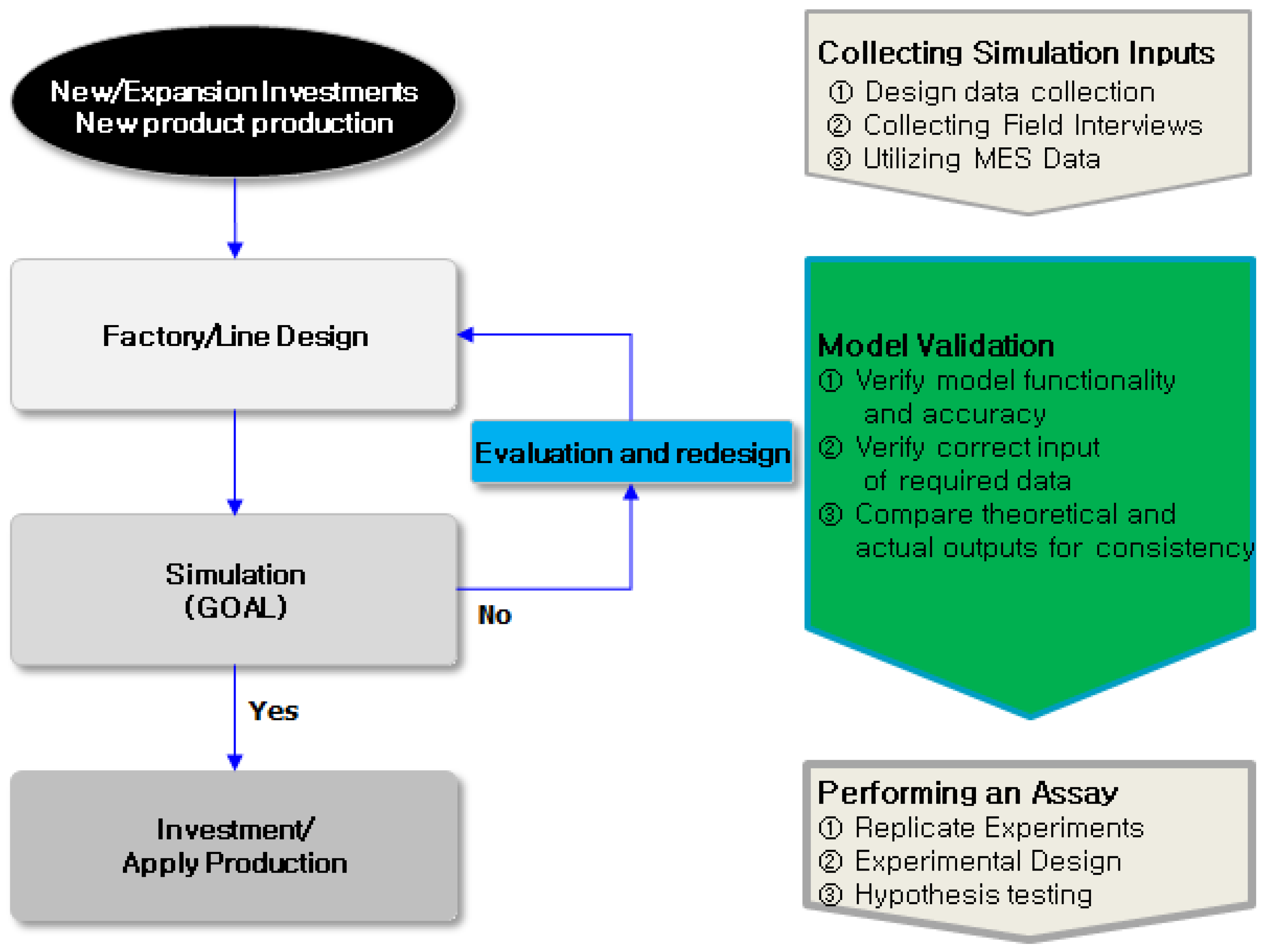
Figure 2.
Reinforcement Learning (RL) Diagram.
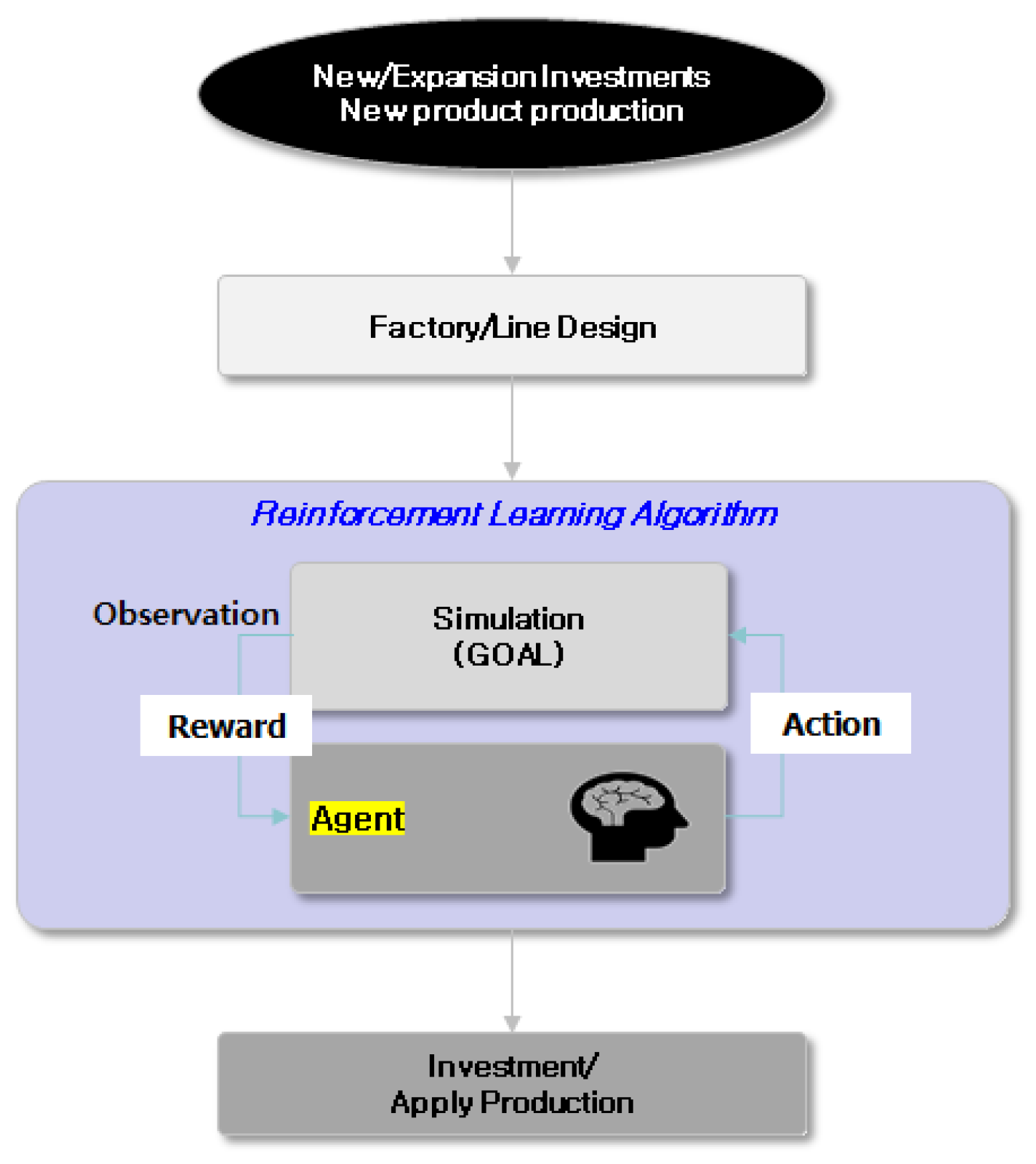
Figure 3.
Manual storage devices.
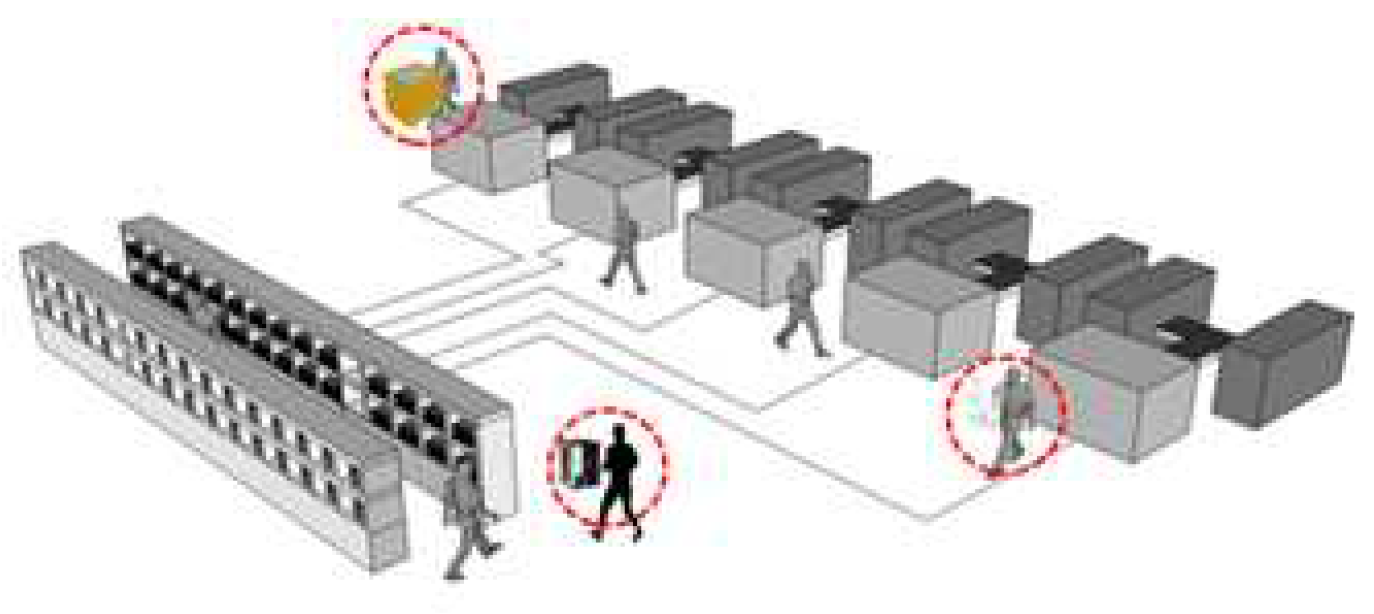
Figure 4.
Automated storage devices.
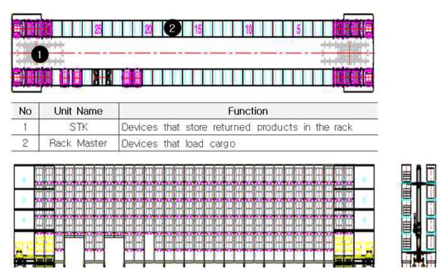
Figure 5.
Single/Double-Deep Racks.
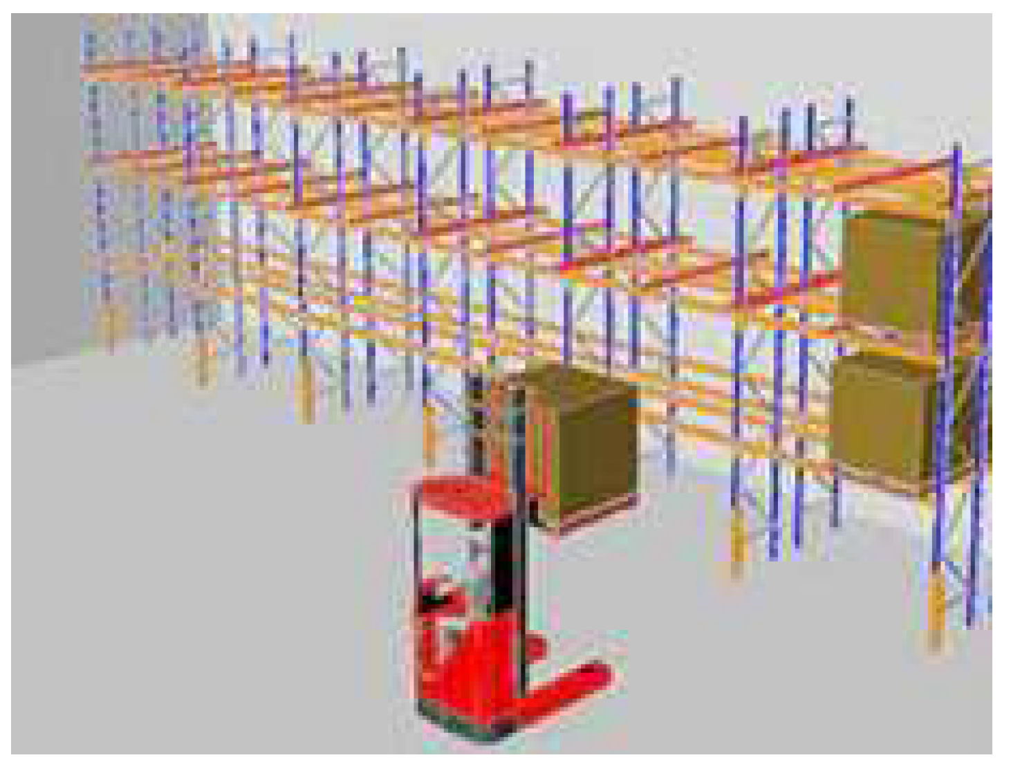
Figure 6.
Drive-in and Drive-thru Rack.
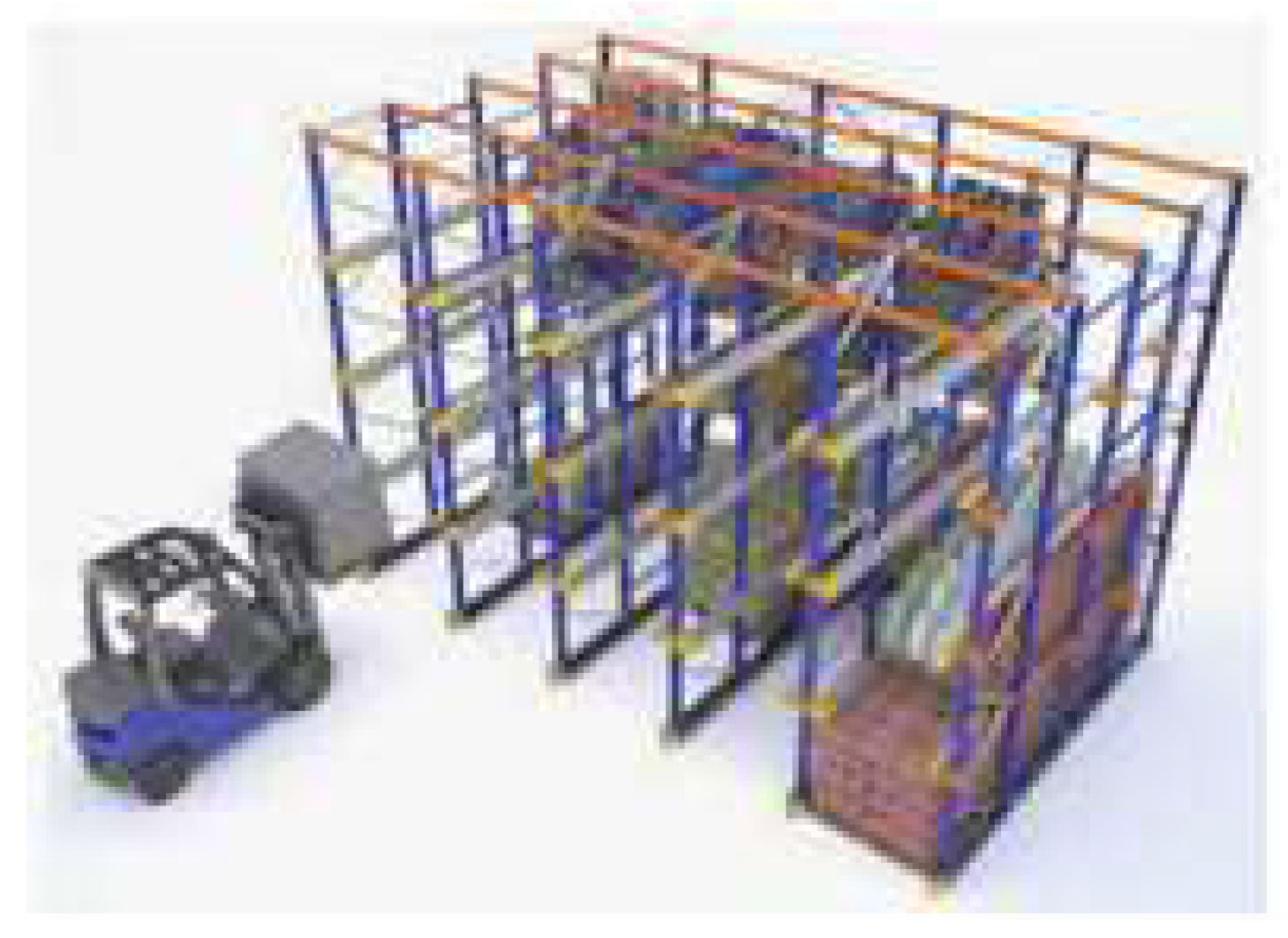
Figure 7.
Carton Flow Rack.
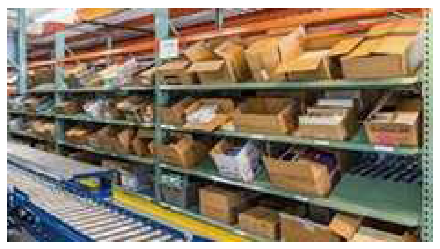
Figure 8.
Pallet Flow Rack.
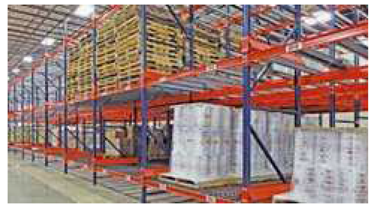
Figure 9.
Push-Back Rack.
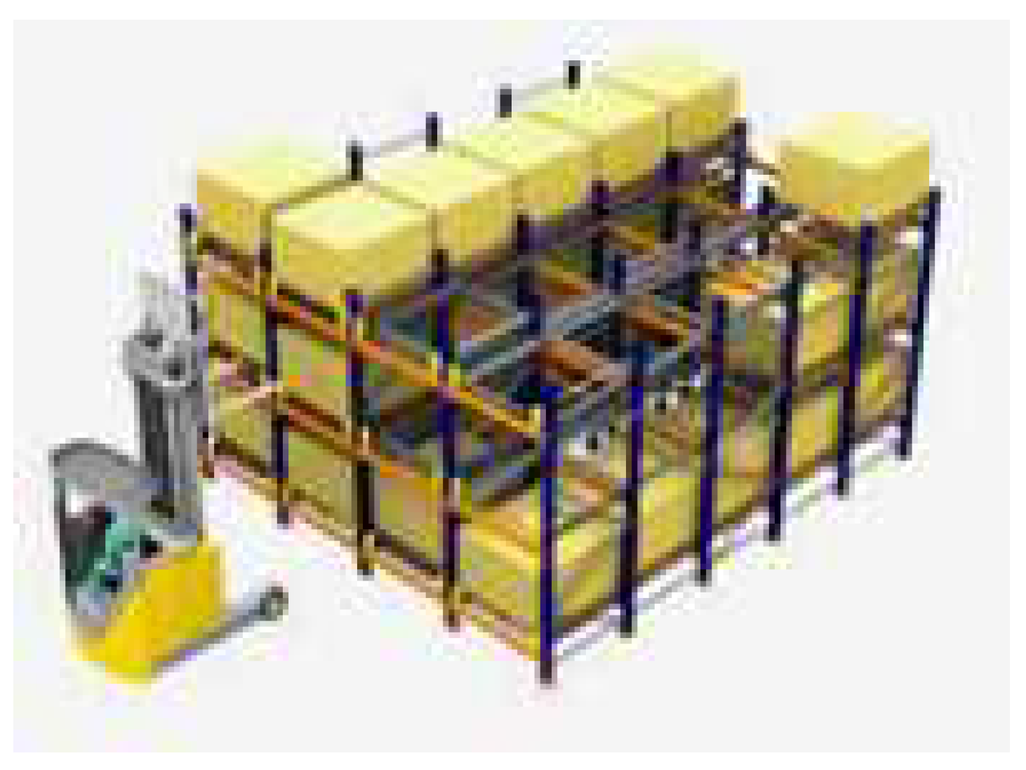
Figure 10.
Mobile Rack.
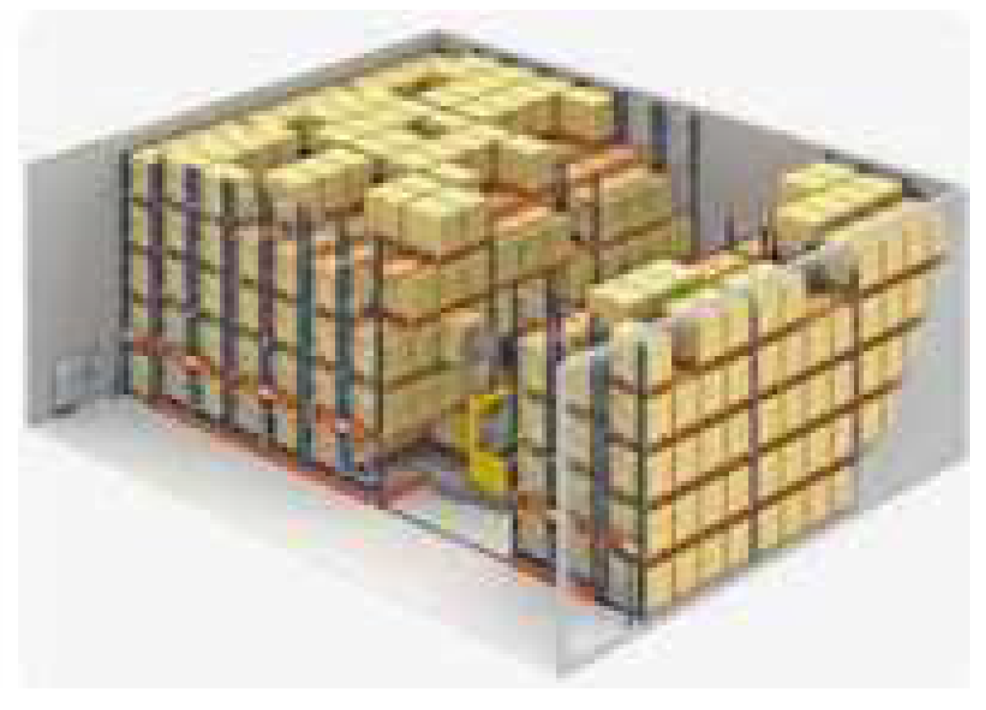
Figure 11.
Factory Simulation Modeling.
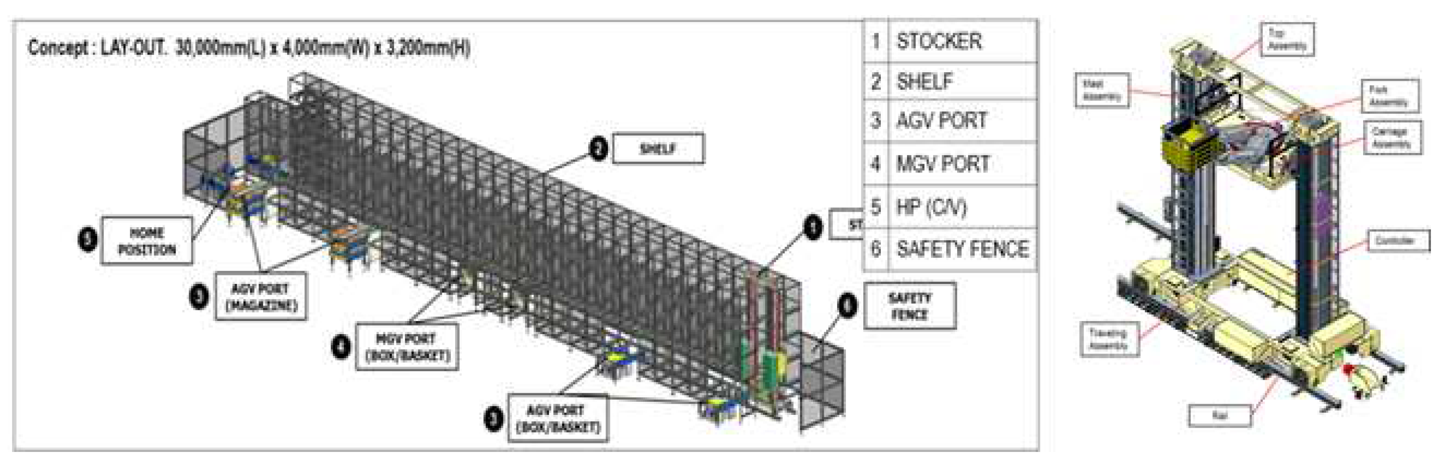
Figure 12.
RL Structure for Factory Simulations.
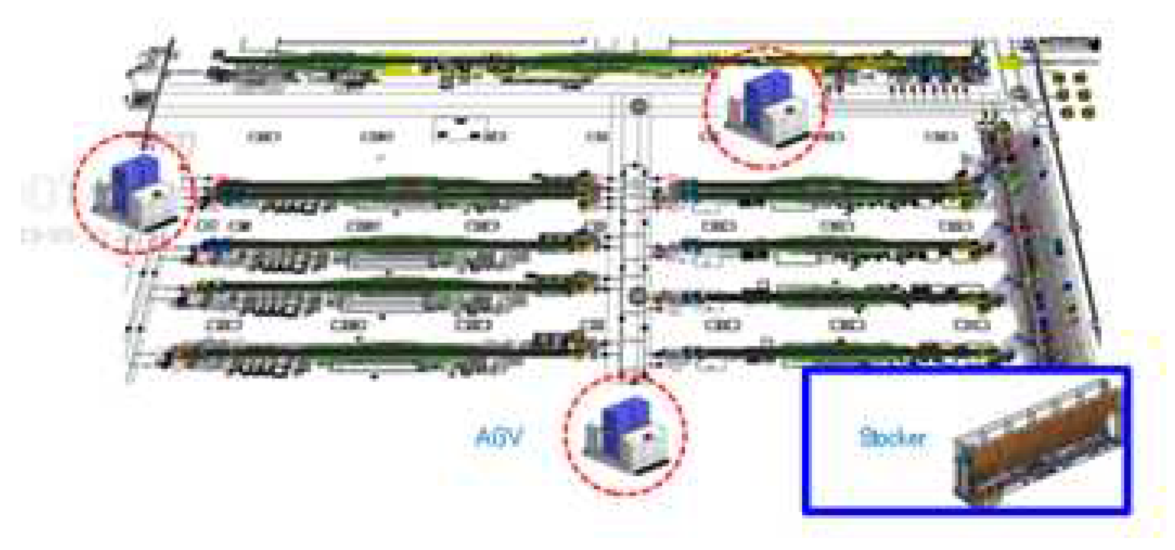
Figure 13.
RL Structure for Factory Simulations.
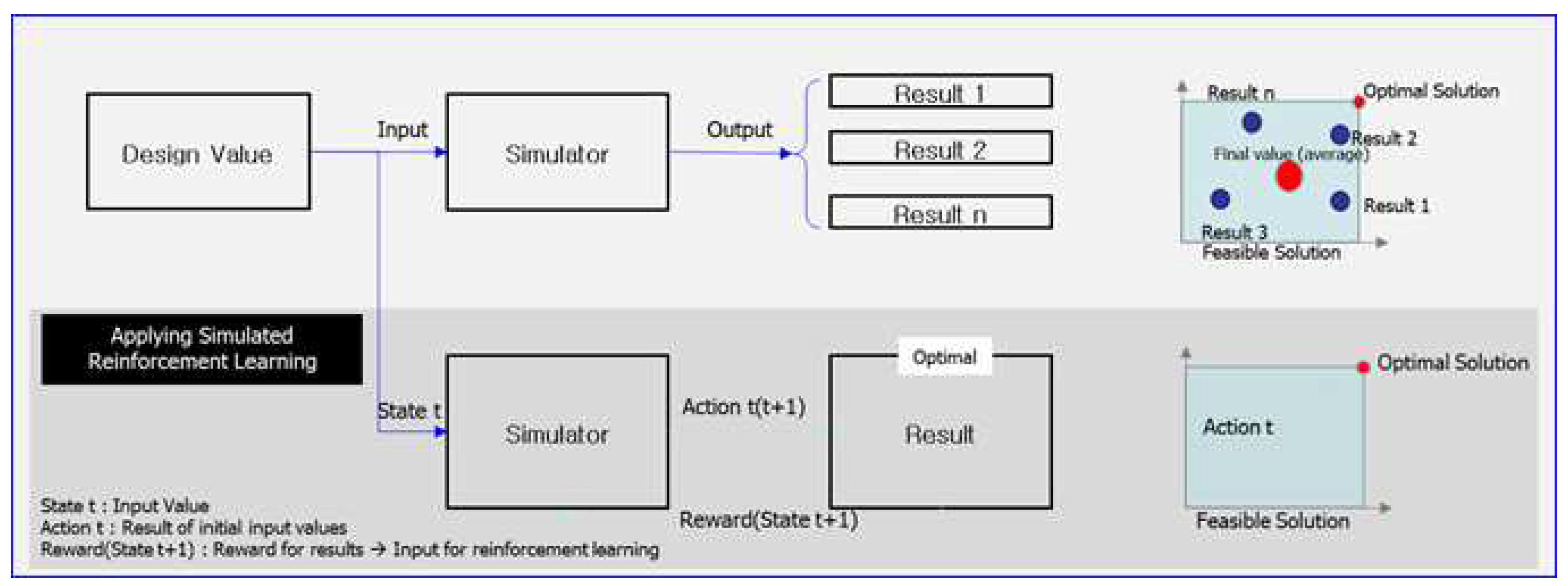
Figure 14.
Virtual Factory Processes.
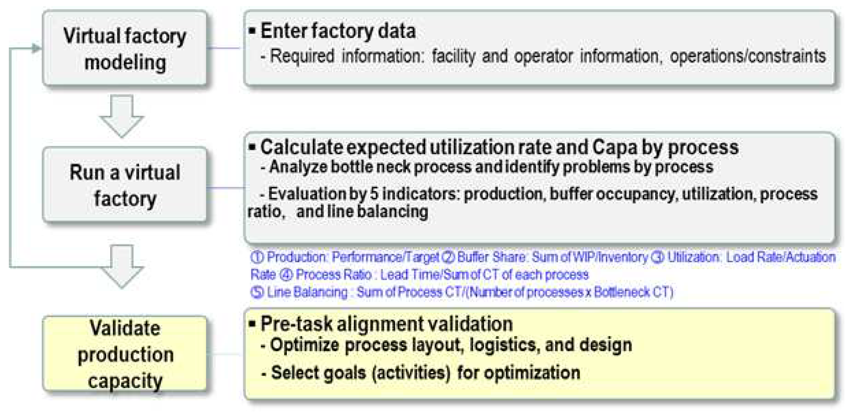
Figure 15.
Organize virtual verification.
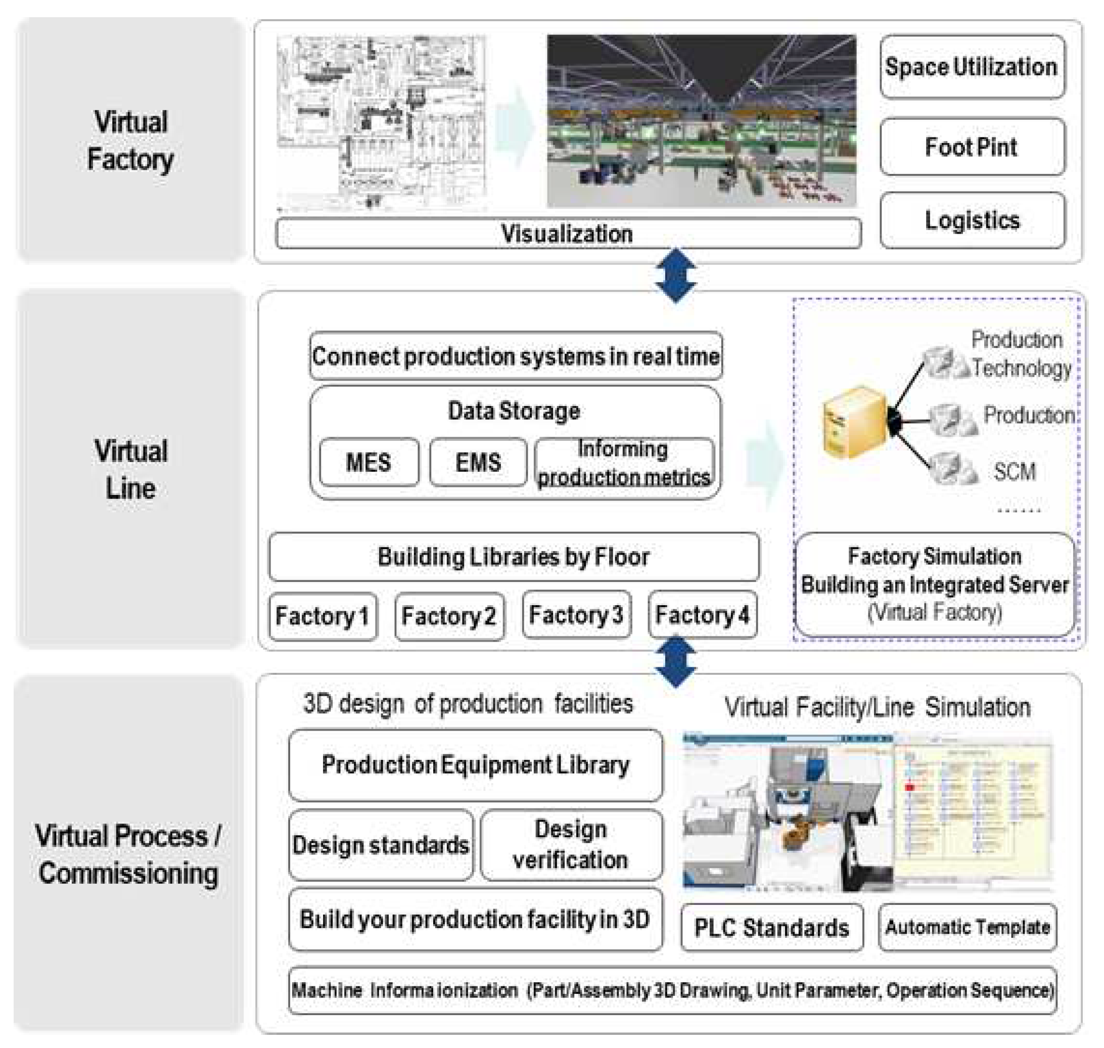
Figure 16.
Factory Simulation Reinforcement Learning Application Block Diagram.
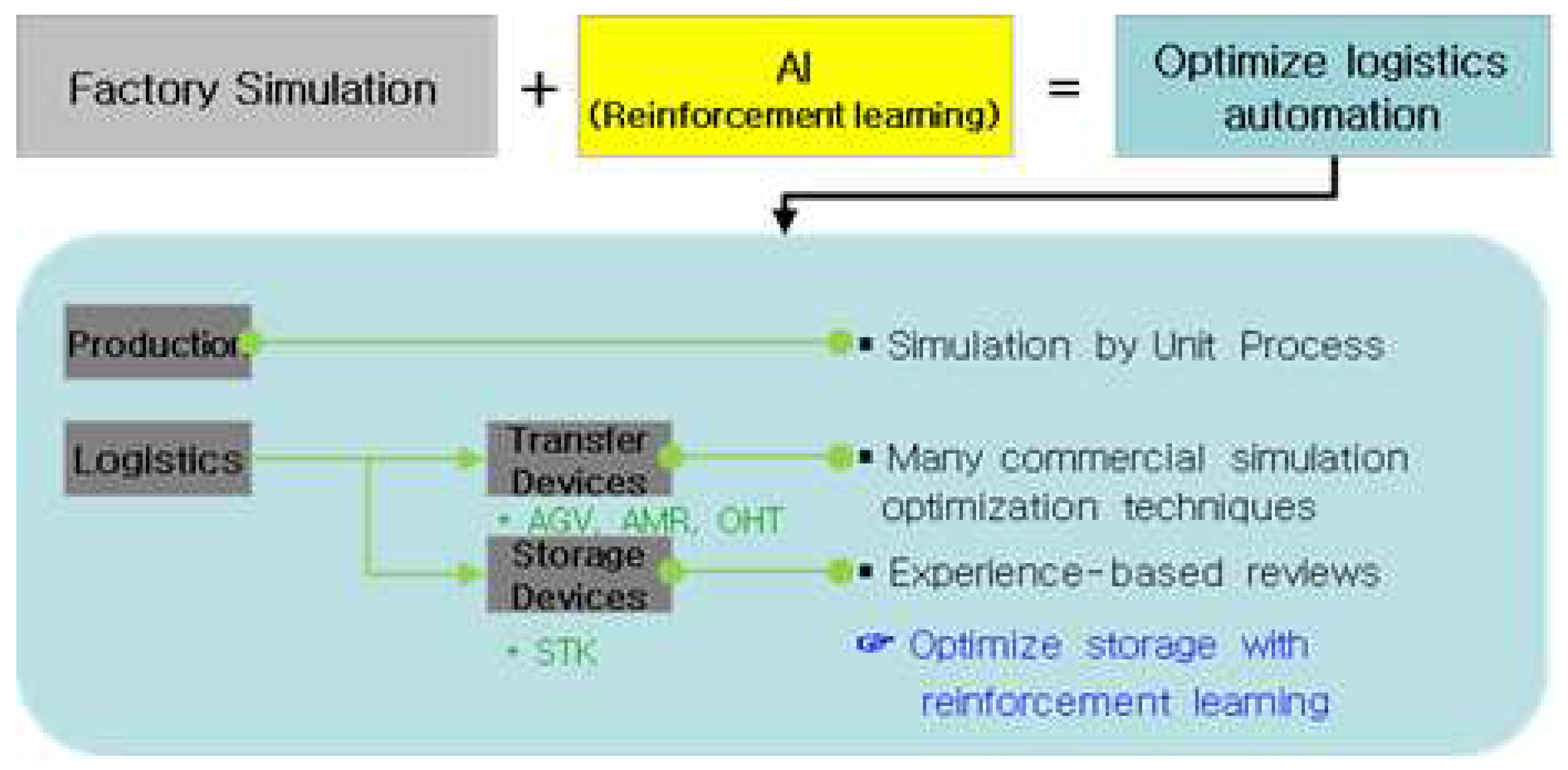
Figure 17.
Factory Simulation System Diagram.
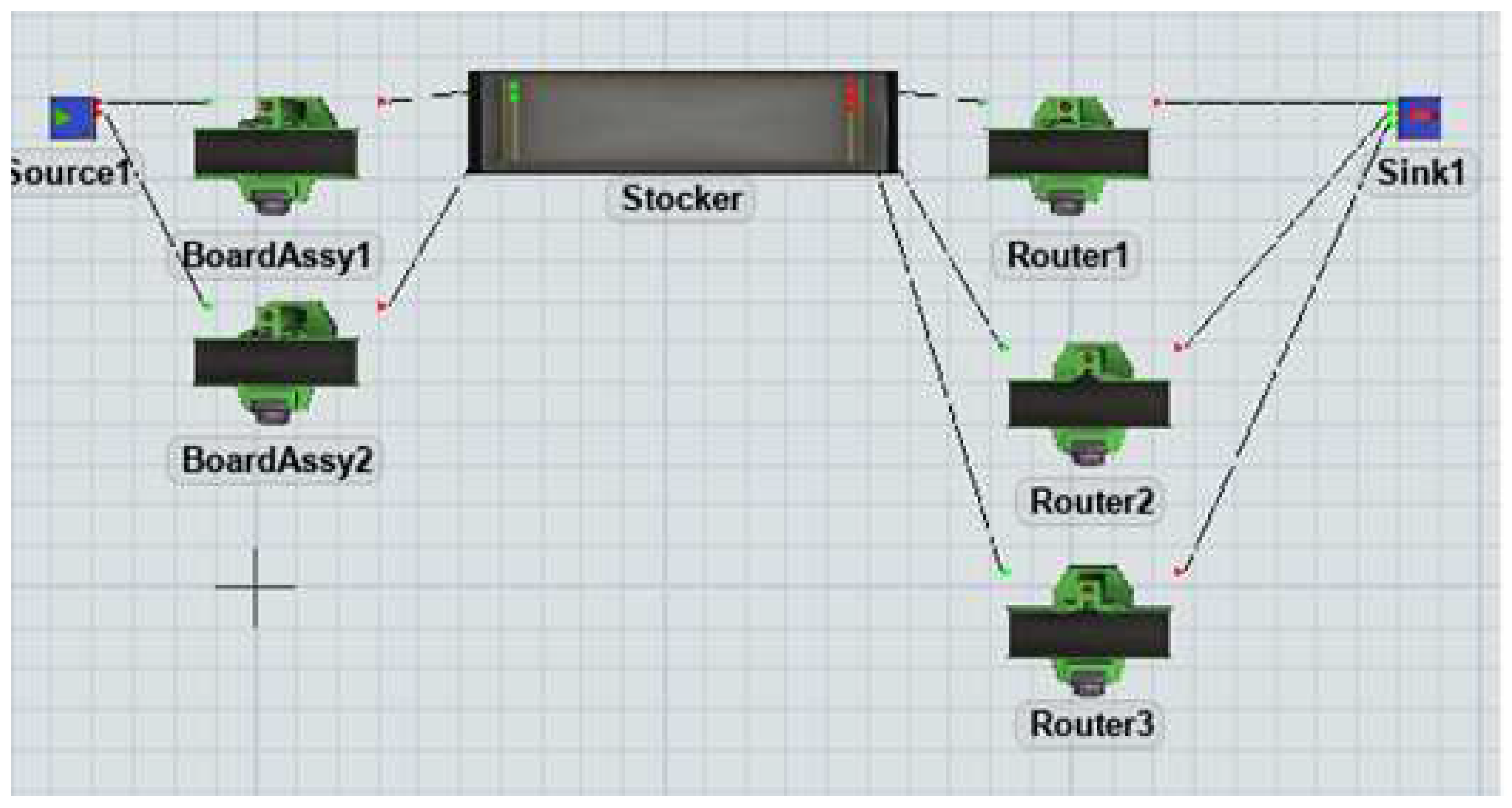
Figure 18.
FIFO type.
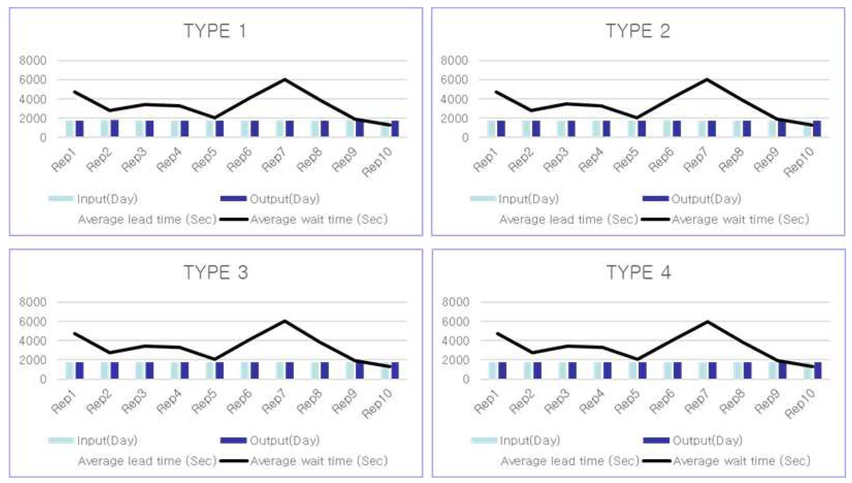
Figure 19.
RL application type.

Figure 20.
Average number of Stocker waiting over training
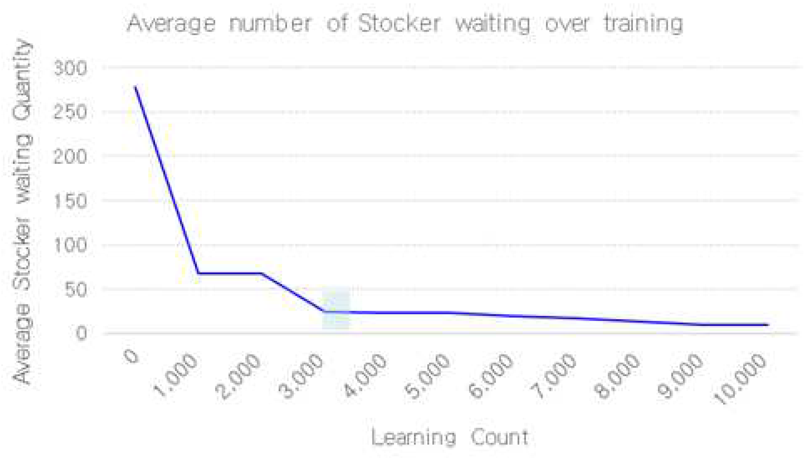

Table 1.
Process time.
| Item | Board Assy | Rounter |
|---|---|---|
| Type 1 | 20 | 19 |
| Type 2 | 17 | 25 |
| Type 3 | 14 | 23 |
| Type 4 | 15 | 21 |
Table 2.
Results by FIFO
| Item | Input | Output | Average | |
| Lead time(S) | Wait time(S) | |||
| Type 1 | 1766 | 1757 | 3351 | 3347 |
| Type 2 | 1760 | 1754 | 3406 | 3349 |
| Type 3 | 1756 | 1749 | 3400 | 3348 |
| Type 4 | 1754 | 1748 | 3400 | 3349 |
Table 3.
FIFO average results
| Item | Input | Output | Average | ||
| Lead time(S) | Wait time(S) | waiting Quantity | |||
| Result | 7034 | 7009 | 3402 | 3348 | 272 |
Table 4.
Results by RL application type
| Item | Input | Output | Average | |
| Lead time(S) | Wait time(S) | |||
| Type 1 | 1767 | 1767 | 159 | 106 |
| Type 2 | 1760 | 1767 | 233 | 176 |
| Type 3 | 1756 | 1756 | 204 | 152 |
| Type 4 | 1766 | 1766 | 198 | 148 |
Table 5.
RL application average results
| Item | Input | Output | Average | ||
| Lead time(S) | Wait time(S) | waiting Quantity | |||
| Result | 7058 | 7058 | 198 | 145 | 12 |
Disclaimer/Publisher’s Note: The statements, opinions and data contained in all publications are solely those of the individual author(s) and contributor(s) and not of MDPI and/or the editor(s). MDPI and/or the editor(s) disclaim responsibility for any injury to people or property resulting from any ideas, methods, instructions or products referred to in the content. |
© 2023 by the authors. Licensee MDPI, Basel, Switzerland. This article is an open access article distributed under the terms and conditions of the Creative Commons Attribution (CC BY) license (http://creativecommons.org/licenses/by/4.0/).
Copyright: This open access article is published under a Creative Commons CC BY 4.0 license, which permit the free download, distribution, and reuse, provided that the author and preprint are cited in any reuse.


