Submitted:
12 June 2023
Posted:
13 June 2023
You are already at the latest version
Abstract
This paper presents research on the application of trajectory design, optimization, and control to an orbital transfer from Mars-Phobos Distant Retrograde Orbits to the surface of Phobos. Given a Distant Retrograde Orbits and a landing location on the surface of Phobos, landing trajectories for which total Δv for a direct 2-burn maneuver is minimized are computed. This is accomplished through the use of Particle Swarm Optimization in which the required Δv and time of flight are optimization parameters. The non-uniform gravitational environment of Phobos is considered in the computation. Results show how direct transfers can be achieved with Δv in the order of ∼30 m/s.
Keywords:
Mars
; Distant Retrograde Orbits
; Phobos
; Particle Swarm Optimization
; landing trajectories
1. Introduction
In order to facilitate the exploration of the Moon and Mars, intermediate staging locations have been proposed. The Lunar Gateway represents an intermediate orbital platform capable of linking, organizing, and supporting missions between the Earth and the Moon [1,2,3]. However, a lesser amount of literature regarding the use of similar platforms in the Martian environment exists. Such Martian platform would be referred to as Mars Base Camp [4]. As well as the Lunar Gateway, Mars Base Camp is a proposed platform that would enable and aid exploration of Mars and its surroundings, including its moons, Phobos and Deimos [5,6,7]. Although a final location for Mars Base Camp has not been chosen, it has been proposed that it could be located in the vicinity of Phobos or Deimos [8], such as a Mars-Phobos Distant Retrograde Orbit (MP DRO) [9]. This would avoid locating Mars Base Camp deep in Mars’ gravity well while keeping the Martian moons an accessible target. Some studies have shown the effectiveness of intermediate staging locations such as the aforementioned Mars Base Camp to facilitate missions in the vicinity of Mars and its moons [10,11]. Thus, the establishment of an infrastructure capable of performing In-Situ Resource Utilization (ISRU) of the material found in the regolith and under the surface of Phobos would prove to increase human and robotic exploration capabilities on Mars and its vicinity. For the purpose of this research, we assumed the existence of a Phobos Base capable of resupplying Mars Base Camp located in a Distant Retrograde Orbit (DRO). We analyzed the necessary trajectories required to transport material from the surface of Phobos to Mars Base Camp. We applied trajectory design, optimization, and control to an orbital transfer in the Circular Restricted Three-Body Problem (CR3BP), specifically from a Mars-Phobos Distant Retrograde Orbit to the surface of Phobos [12]. Given an MP DRO and a landing location on Phobos, the goal is to find the trajectory for which total for a direct 2-burn maneuver is minimum [8,13]. Here, the total corresponds to the sum of ’s required to initiate the transfer in the MP DRO and complete the transfer, i.e. land on the surface of Phobos. Considerations on Time-Of-Flight (TOF) were done in order to ensure that any necessary phasing and/or repositioning maneuvers are taken into account. A 2-D analysis is sufficiently accurate since we considered the Mars-Phobos orbit plane as the reference frame, and motion will mostly happen in such plane. However, further analysis will take into account a 3-dimensional space problem in which the gravitational potential of Phobos is also considered [14]. Furthermore, the initial position among the departing DRO will be implemented as the third optimization parameter, given that the minimum does not necessarily occur at a fixed position along the orbit for a given landing location. In this paper, a Particle Swarm Optimization (PSO) is used to determine the initial MP DRO given two parameters, . Once the initial DRO is found, a trajectory optimization through a PSO is performed in order to determine the lowest trajectory to land a specific location on Phobos’ surface, given three parameters to optimize . Here, we also discuss which PSO parameters are used for the analysis and which ones lead to the most efficient (i.e., the fastest) computations, that can be used for other optimization problems in the CR3BP. For further details on such parameters, refer to the nomenclature session at the beginning of the paper or to the detailed Section 2.3 and Section 3.
Phobos is the largest of two moons orbiting Mars, with an approximate size of km km km [15,16]. Phobos has an unusual shape (somewhat similar to a potato) which creates numerous difficulties for spacecrafts to orbit and therefore land on the moon itself. In the literature, the gravitational potential and the density of Phobos have been of high interest, since it becomes essential for a precise and complete analysis to acknowledge such characteristics, especially for long-duration stability of orbits in the vicinity of the Moon [17,18,19].
In this paper, the following approximations are made. Phobos orbits Mars on an elliptical orbit with an eccentricity of . For this study, we modeled Mars and Phobos using the CR3BP, which assumes that the eccentricity is 0. The semi-major axis of such orbit (i.e. average distance between Mars and Phobos) is 9376 km. Finally, the orbit’s inclination with respect to Mars’ equatorial plane is around 1°. Since Phobos’ Sphere of Influence (SOI) is below its physical surface, it becomes impossible to orbit the moon in the classical Keplerian sense. In the CR3BP, considering Phobos and Mars as the two primary masses, some periodic orbits exist, such as Halo Orbits or Lyapunov Orbits, as shown in Figure 1. However, such periodic orbits are either highly unstable or come dangerously close to the surface [20]. That being considered, the family of Distant Retrograde Orbits is of use in the following analysis. Such family of orbits proved to be “far” enough from Phobos’ surface and to be sufficiently stable as well, up to multiple hundreds of years, when considering a full-force model [20]. The word “far” is here used loosely, since these orbits are within tens of hundreds of km from Phobos.
Mission analysis for Earth to Mars-Phobos DROs is of high interest when associated with human and robotic exploration [4,10,11,16]. Phobos could prove itself extremely useful for future Mars missions as a popular location for future ISRU plants. It is widely recognized that having such in-orbit and in-situ infrastructures would make space exploration much more affordable, sustainable, and effective [16,21,22]. Several advantages of such stations include the ability not to bring all the necessary material, including propellant, for deep space missions [23]. Such projects are already in development (such as NASA’s Artemis [24]) for what concerns Earth’s Moon: building a refueling in-orbit station along with several on-the-surface infrastructures can easily be imagined as an intermediate step to what would be a deep space exploration mission.
In the following analysis, optimization algorithms are developed in order to generate a specific DRO given a desired distance from Phobos and optimize a landing maneuver to a specific landing site on the surface of Phobos with respect to the needed, i.e. minimize the necessary impulsive maneuver applied for landing.
2. Background Theory
For the purpose of giving a better insight of the problem, a brief overview of the basic aspects regarding Distant Retrograde Orbits and the Particle Swarm Optimization method are given.
2.1. Distant Retrograde Orbits
Distant Retrograde Orbits (DROs) are large orbits around the smaller primary body in the 3BP. Perfectly periodic DROs exist in the CR3BP and in-plane velocity perturbations create quasi-periodic orbits. Such orbits are favorable when looking for quarantine orbits since their stability demonstrates a noteworthy capability to resist perturbations [22]. Indeed, DROs can stay quasi-periodic when larger perturbations than other families of three-body orbits can withstand are applied. DROs have been recently proposed to be the ideal family of orbits when it comes to locating in-space infrastructures, and this is due to their outstanding stability and ease of access in terms of a gravity well [22]. DROs are usually characterized by the so-called x-amplitude (), which represents the larger distance from (in a CR3BP) in the x-axis direction, given a rotating reference frame orbiting the primaries, as shown in Figure 2. In such analysis, it is typical to use a frame of coordinates with its center located at the barycenter of the primary masses [16]. According to this, several essential parameters can be determined in order to define a DRO. Such parameters are the radius at periapsis, and its corresponding velocity, required at the intersection of the -plane (i.e. where ) in order to create a periodic orbit. Since the radius has only one component along the x-axis, which is -dependent, we can say that the essential parameters necessary to define a DRO are , where indicates the y-component of the velocity vector at such location (which is in facts the only component, the x-component and z-component of the velocity vector at the considered starting location are zero). DROs have been identified and studied in the literature, for both Earth-Moon DROs and Mars-Phobos DROs [16,25], as shown in Figure 3. However, in this study a PSO algorithm will be used to determine a DRO given its x-amplitude, which will be the starting point for the landing trajectory optimization.
2.2. Particle Swarm Optimization
The Particle Swarm Optimization method is used in this study as an optimization algorithm to generate periodic DROs and compute -optimal landing trajectories. PSO is a heuristic method used several times in previous astrodynamics problems [26,27,28]. It is based on the unpredictable motion of bird flocks while searching for food, taking advantage of the mechanism of information sharing that affects the overall behavior of a swarm [29,30]. The initial population that composes a swarm is randomly generated at the first iteration of the algorithm. Each particle is associated with a position vector and a velocity vector. In the PSO terminology, the words “position” and “velocity” are not to be interpreted in the classical sense (i.e. position and velocity as intended in classical physics and mechanics). Instead, they indicate the position vector containing the unknown parameters to optimize and the velocity vector determining the position update. Each particle represents a possible solution to the problem. At the end of the iterations, the particle corresponding to the optimal solution is selected, i.e. the particle that minimizes the parameters of interest, such as . At each iteration, the position vector’s elements move in the velocity vector’s corresponding direction, to a new position, which represents a new possible solution. The updating of position and velocity is based on the objective function evaluation at the end of every iteration. The objective function (henceforth referred to as “cost function”) is an expression that needs to be minimized (or maximized). Once this condition is satisfied or the maximum number of iterations set is reached, the algorithm will have obtained an optimal solution. At every iteration, the best cost function is used to determine how to update both velocity and position. Indeed, with the approach formulated above, the algorithm will converge on the best solution in every iteration. For each particle, the formula for velocity update includes three components with stochastic weights. In the PSO terminology, these are known as the inertial (), cognitive (), and social () components. The inertial parameter is usually chosen randomly, but it has appeared to be proportional to each particle’s velocity in the previous iteration for some applications [28]; the cognitive parameter is based on the best position experienced by the particle; finally, the social component is direct toward the personal best position (i.e. the best location yet located by any particle in the swarm). The algorithm terminates when the maximum number of iterations (user decision) is reached. For this study, the following values are used in the algorithm. The function rand stands for a single uniformly distributed random number in the interval (0,1).
The constants in Equation (1) are derived from the literature and optimized for this problem [31,32]. The implementation of the PSO was run in MatLab where the function unifrnd was used to assign the initial values at each particle element for each particle. The function unifrnd creates a uniformly distributed array of random values included in a specific range as given by the boundary values in Table (Table 2). Once that is implemented, the initial position is assigned
where
represents the mass ratio. Note that, as already mentioned, the following analysis will be conducted assuming 2-D motion. Therefore the particle (i.e. the particle corresponding to the iteration) is
so that
The PSO algorithm here used is summarized in the flowchart in Figure 4. The coordinate system used is represented in Figure 5. Note that these two parameters are picked for the MP DRO analysis described in the Mars-Phobos DRO section below and are here used to better describe the general problem and give the reader a full comprehension of the general approach. Once the Initial Conditions (ICs) are determined ( and ), numerical integration is performed in order to compute the resulting trajectory using the CR3BP equations:
Once the integration is done, if the final position and velocity of the resulting trajectory are within a small tolerance (here ) to the initial conditions and , then a periodic orbit is achieved and the optimization algorithm has reached a final solution.
Therefore, the cost function, i.e. function to minimize, is
Satisfying the condition in Equation (8) results in having a periodic orbit, i.e. and . Once the cost function is evaluated, each particle velocity (intended in the PSO terminology) is updated as follows
where is the personal best of each particle, and is the overall best position between all particles and all iterations as of the iteration. The coefficients are defined in Equation (1). Note that the subscript i in the Equations (4, 8, 9) indicates the element at the iteration of the algorithm. Naturally, the greater number of particles initialized, the more probability the algorithm has to achieve an optimal result. Similarly, a higher number of maximum iterations has more probability to converge to a solution. Nevertheless, a compromise between computational complexity and the number of iterations and particles needs to be made. In fact, increasing either the number of particles or the maximum iterations allowed can make the computational time increase significantly. However, due to the random nature of the algorithm, one cannot guarantee that an absolute optimal solution can be reached. On the other hand, a `good’ initial guess is not necessary in order to initiate the algorithm. Furthermore, unlike gradient-based methods, heuristic optimization methods are capable of finding absolute maxima/minima regardless of ICs [31].
2.3. Mars-Phobos DRO
Several DROs have been defined in the literature [12,16] for given values. Here a PSO algorithm has been implemented to generate DROs. The optimization was implemented starting from the two parameters [T,], where was defined in Section 2 and T represents the orbital period of the DRO. The initial data are summarized in Table 1.
Starting from data taken from [16] the value of for km is known to be km/s, that identifies a DRO with an orbital period s [33]. Knowing such parameters helps the implementation of boundary values for the two parameters used in this analysis (i.e. the maximum and minimum values that the parameters can assume in the particles). In particular, the initial conditions for the optimization are listed in Table 2. Similarly, any other DRO of interest can be derived, although only one is here chosen for the results shown.

Table 1.
Orbital parameters for Mars-Phobos and initial values for DRO Optimization.
| Variable | Value | Description |
|---|---|---|
| (km3 s−2) | Gravitational parameter for Phobos |
|
| (km3 s−2) | Gravitational parameter for Mars |
|
| Mass ratio | ||
| R (km) | 9376 | Average distance Mars-Phobos |
| (km) | 125 | DRO Amplitude |
Table 2.
Boundary Values for DRO Optimization.
| Variable | Value | Description |
|---|---|---|
| () | Lower limit for (km/s) | |
| () | Upper limit for (km/s) | |
| () | T | Lower limit for T (s) |
| () | Upper limit for T (s) | |
| 80 | Maximum number of iterations | |
| 40 | Number of particles |
The parameters to optimize are the initial velocity (Equation (5)) at position (Equation (2)) and the orbital period T (Equation (4)). In the literature, different DROs have been identified for km [16]. DROs with values below 15 km result in a certain impact with Phobos’ surface and the ones with higher values than 300 km are considered too far away to maintain the characteristics in which we are interested (vicinity to Phobos and low- for landing). Given the initial orbital parameters for Mars-Phobos and the initial values for the DRO, specified in Table 1, the resulting DRO is shown in Figure 6, and its reference values for position and velocity are summarized in Equation (10).
where T represents the total orbital period, and v is the velocity vector at position r. Given the and specified in Table 2, the result was achieved with a minimum cost function J in the order of approximately, as shown in Figure 7, so the final values are such that 0.1 mm and 0.1 mm/s . The total average computation time was ∼20 seconds. Several other approaches were tried, in terms of the number of particles and the number of maximum iterations, but these parameters proved to give a sufficiently accurate result in a reasonable amount of time. If, for instance, we doubled the up to 160, the computation time increases up to ∼40 seconds, generating a minimum cost function J in the order of . So doubling the computational time will generally give a result that is just one order of magnitude more accurate than the initial one. As already outlined, one has to compromise between computational efficiency, computational speed, and results’ accuracy.
Many computational issues may occur while implementing the algorithm. However, parallel programming and computing is a suitable solution to speed up the computation time. In fact, every possible trajectory computed at each iteration is independent with respect to all the other trajectories, until every particle is updated. Note that for this study a 2016 MacBook Pro is used. Hardware and Software details are summarized in Table 3.
3. Landing Trajectory Optimization
In this section, the trajectory optimization for multiple landing maneuvers is analyzed through the use of PSO. Given an initial stable parking DRO around Phobos like the example computed in Section 2.3, and a desired landing location, the analysis aims to find the minimum necessary to encounter that specific location. The problem is computationally more complex than the one described in the MP DRO Section and it presents several more difficulties in the formulation. First of all, the choice of the parameters to optimize is non-trivial and there are different ways to approach the optimization. Here, the following parameters were chosen, minimizing the dimensionality of the trade space to three:
where the element represents the to apply, and indicates the angle with respect to the x-axis at which the is applied. The parameter represents the angle with respect to the x-axis which consequently identifies a location on the DRO , as shown in Figure 8. Note that in this analysis, the index i represents the particle at the iteration. This analysis requires more computational time than the DRO optimization because there are 3 parameters to optimize instead of 2, and we do not have specific analytic expressions to relate them to each other. The starting DRO is equal to the one defined in the optimization described in Section 2.3. Therefore, as obtained in Equation (10), the initial values and the particle boundary values are summarized in Table 4 and Table 5 respectively.
In this particular optimization, a penalty scaling factor was introduced. The addition of such a factor is necessary in order to prioritize the terms of the cost function [34]. In fact, the essential condition for a valid outcome of the optimization is to land at the desired location on Phobos. Indeed, a trajectory is considered valid only if it intersects the surface of Phobos. Secondarily, given that a valid trajectory to accomplish such a condition has been found, the total needs to be minimized. The expression for was derived in the literature [34], and the following proved to be an effective value for this factor
where i is the current iteration number, is the maximum number of iterations and and represent the initial and the final weighting values. In this analysis, they are equal to 1 and 0.1 respectively. The factor is an order scaling factor, set equal to 100 for this optimization, which is used to make sure that the location checking term has a higher order than the term. Therefore, the cost function becomes
For this optimization, the tolerance (tol) is set to 0.1 km (100 meters). It is clear how the scaling factor prioritizes a specific term in Equation (13), given that the term is a relatively small value.
For a matter of simplicity, Phobos was ideally divided into 12 sectors, and a landing location within each sector was picked as a reference location for such area. This means that the required to achieve landing in such sector can be considered quantitatively similar to the reference location’s . Results for the landing locations in each sector are summarized in Table 7. Computation times for each example in Table 7 are indicated in Table 6. As expected, the average computation time is slightly higher than the one for the DRO optimization described in the MP DRO analysis.
The landing trajectories for each sector are represented in Figure 10 and a heat map of all the landing locations is shown in Figure 9. To have a better insight into the results, a fully loaded SpaceX Starship is considered. SpaceX’s Starship will have an empty mass of ∼120 mt (260,000 lb) and a gross mass of ∼1,320 mt (2,910,000 lb) with a propellant capacity of ∼1,200 mt (2,600,000 lb)[35]. Recall the Tsiolkovsky rocket equation
where is the total mass of the spacecraft, including the propellant, is the final total mass assuming all propellant to be consumed (also known as dry mass), is the spacecraft’s specific impulse and is the standard gravity at Earth’s sea level. We can now assume to land on Phobos’ surface at sector 7, which latitude corresponds to the Stickney Crater on the surface of Phobos and which corresponds to a total of 27.41 m/s (see Table 7). From Equation (14) we can estimate the necessary propellant mass to land a full-load Starship on Phobos.
We consider the spacecraft to empty its tanks at landing. Given a specific impulse of 380 s in a vacuum and a payload of 100 mt, Starship will achieve landing with a total propellant mass equal to
where is the total propellant mass used to achieve the indicated . Since the landing is quantitatively equal to the required to go from the surface of Phobos to the initial DRO (the trajectory will just look different from a qualitative point of view), and we assumed Phobos to have a re-fueling station on its surface, the total propellant mass necessary to leave and arrive the DRO is simply two times the mass indicated in Equation (15). Therefore, assuming one travel per terrestrial day for a year (365 days) back and forth the Stickney Crater, the total propellant mass per year necessary to achieve such transfers is ∼1,185.22 mt of propellant. If we consider a 1,200 mt propellant capacity, Starship can achieve a back-and-forth transfer ∼369 times before refueling. Although it is challenging to precisely estimate the propellant price per tonne, SpaceX claims that refueling Starship would cost approximately $900,000. This means that a complete transfer would cost around $2,435, transporting a 100 mt payload.
4. Conclusions
This study led to valuable results for both DRO implementations and landing trajectory optimization. Several DROs have been defined in the literature for given values, but not much exists about landing trajectories from DROs to the surface of Phobos. Regarding the landing trajectory optimization, which is the main purpose of this study, it is clear from Table 7 how the is on average equal to ∼30 m/s. This value is reasonably low and makes this orbit feasible for an in-orbit refueling station or in general for a stationary orbit around Phobos which one can easily reach and leave. Several landing locations were reached, and the impulsive was always found to be in approximately the same range. Therefore, nearly every point on Phobos’ surface can be reached with a of approximately ∼30 m/s. Furthermore, as summarized in Table 6, the average computation time for such PSO algorithm is reasonable and makes the optimization feasible for future mission designs.
Mars’ moons exploration has been of high interest within the scientific community in the past years. The existence of periodic orbits around Phobos, such as DROs, makes the future design of in-orbit refueling and supporting stations more than feasible. Moreover, the ease of departing and arriving to such orbits with low ’s gives the possibility of exploring Phobos and establishing a Mars Base Camp, in order to explore Mars and its surroundings with great versatility and with lower flight times between transfers from and to Mars itself. Having stations or spacecrafts orbiting around Mars (in Low-Mars Orbits for example) would require continuous trajectory adjustments because of Mars’ gravity potential acting on the spacecraft/station, and will then result in significant used over the course of a long-term mission. Besides, given the distance between Earth and Mars, it would not be convenient to perform frequent trajectory adjustments or remote control operations, given an average transmission delay of ∼20 minutes between Mars and Earth. Hence, having a long-term stability solution is crucial, and DROs appear to be feasible for such an objective. The method here presented can be used for multiple Mars-Phobos DROs optimizations at different amplitudes. Plus, a Mars-Deimos DRO can utilize this very same approach.
Author Contributions
Vittorio Baraldi is the primary author and researcher of this paper who developed the mathematical tools and performed all major calculations presented in the paper. Dr. Davide Conte is Vittorio’s faculty advisor, who helped guide Vittorio’s research work and reviewed the content and writing of this paper through multiple rounds of reviews. Conceptualization, Vittorio Baraldi and Davide Conte; Formal analysis, Vittorio Baraldi; Methodology, Vittorio Baraldi; Project administration, Davide Conte; Supervision, Davide Conte; Writing—original draft, Vittorio Baraldi;Writing—review&editing, Davide Conte.
Funding
This research received no external funding.
Informed Consent Statement
Not applicable.
Conflicts of Interest
The authors declare no conflict of interest.
Nomenclature
| Change in velocity (km/s) | |
| e | Orbit eccentricity |
| Larger x-coordinate from the primary body in the Circular Restricted Three-Body Problem (km) |
|
| y-component of velocity (km/s) | |
| Maximum number of iterations used in Particle Swarm Optimization (PSO) |
|
| T | Orbital Period (s) |
| Number of particles used in PSO | |
| J | Cost function |
| Mass ratio of Mars and Phobos | |
| Position vector | |
| Velocity vector | |
| Number of particles in PSO | |
| Lower limit for particles in PSO | |
| Upper limit for particles in PSO | |
| Angle with respect to the x-axis at which the is applied (°) | |
| Position along the orbit with respect to the x-axis, starting at (°) | |
| Initial position vector | |
| Initial velocity vector | |
| Final position vector | |
| Final velocity vector | |
| Penalty scaling factor used by PSO | |
| Gravitational parameter (km3/s2) | |
| Total spacecraft mass (mt) | |
| Dry spacecraft mass (mt) | |
| Propellant mass (mt) | |
| Specific Impulse (s) | |
| Standard acceleration due to gravity at Earth’s sea level (m/s2) | |
| Exhaust velocity (m/s) |
References
- Loff, S. Lunar Gateway. 2012. Available online: https://www.nasa.gov/topics/moon-to-mars/lunar-outpost (accessed on 12 April 2020).
- Johnson, S.K.; Mortensen, D.J.; Chavez, M.A.; Woodland, C.L. Gateway – a communications platform for lunar exploration. In Proceedings of the 38th International Communications Satellite Systems Conference (ICSSC 2021), Vol. 2021; pp. 9–16. [Google Scholar] [CrossRef]
- National Aeronautics and Space Administration (NASA) White Paper: Gateway Destination Orbit Model: A Continuous 15 Year NRHO Reference Trajectory. 2019.
- JAXA. Martian Moons Exploration: Mission Overview. http://www.isas.jaxa.jp/en/topics/files/MMX170412_EN.pdf, 2017.
- Ulamec, S.; Michel, P.; Grott, M.; Boettger, U.; Hübers, H.W.; Schröder, S.; Cho, Y.; Rull, F.; Murdoch, N.; Vernazza, P.; et al. Surface science on Phobos with the MMX Rover. 2022.
- Adams, E.; Murchie, S.; Eng, D.; Chabot, N.; Guo, Y.; Arvidson, R.; Trebi-ollennu, A.; Seelos, F. Mission concept for robotic exploration of Deimos. 61st International Astronautical Congress 2010, IAC 2010 2010, 11, 9249–9259. [Google Scholar]
- Ulamec, S.; Michel, P.; Grott, M.; Boettger, U.; Hübers, H.W.; Cho, Y.; Rull, F.; Murdoch, N.; Vernazza, P.; Biele, J.; et al. The MMX Rover Mission to Phobos: Science Objectives. 2021.
- Hopkins, J.; Pratt, W. Comparison of Phobos and Deimos as Destinations for Human Exploration, and Identification of Preferred Landing Sites. AIAA Space 2011 Conference and Exposition 2011. [Google Scholar]
- Martin, L. Lockheed Martin: Mars Base Camp. https://www.lockheedmartin.com/en-us/products/mars-base-camp.html, 2012. Accessed: 2020-04-12.
- Cichan, T.; Norris, S.; Chambers, R.; Jolly, S.; Scott, A.; Bailey, S. Mars Base Camp: A Martian Moon Human Exploration Architecture. AIAA Space 2016 Conference and Exposition 2016. [Google Scholar]
- Chican, T.; Bailey, S.; Antonelli, T.; Jolly, S.; Chambers, R.; Ramm, S. Mars Base Camp: An Architecture for Sending Humans to Mars. New Space 2017, 5. [Google Scholar]
- Conte, D. Determination of Optimal Earth-Mars Trajectories to Target the Moons of Mars. The Pennsylvania State University (Department of Aerospace Engineering).
- Bezrouk, C.; Parker, J. Ballistic Capture into DROs around Phobos: an Approach to Entering Orbit around Phobos without a Critical Maneuver near the Moon. Celestial Mechanics and Dynamical Astronomy 2018, 130. [Google Scholar] [CrossRef]
- Fraeman, A. Analysis of Disk-Resolved OMEGA and CRISM Spectral Observation of Phobos and Deimos. Journal of Geophysical Research: Planets 2012, 117, 1991–2012. [Google Scholar] [CrossRef]
- Wessen, A. Phobos: by the numbers. Available online: http://solarsystem.nasa.gov/moons/mars-moons/phobos/by-the-numbers/ (accessed on 15 March 2020).
- Conte, D.; Spencer, D. Mission Analysis for Earth to Mars-Phobos Distant Retrograde Orbits. Acta Astronautica 2018, 151, 761–771. [Google Scholar] [CrossRef]
- Borderies, N.; Yoder, C. Phobos Gravity Field and its Influence on its Orbit and Physical Libration. Astronomy and Astrophysics 1990, 233. [Google Scholar]
- Shi, X.; Willner, K.; Oberst, J.; Ping, J.; Ye, S. Earth-Mars Transfers through Moon Distant Retrograde Orbits. SCIENCE CHINA: Physics, Mechanics, and Astronomy 2012, 55. [Google Scholar]
- Maistre, S.L.; Rivoldini, A.; Rosenblatt, P. Signature of Phobos’ Interior Structure in its Gravity Field and Libration. Icarus 2019, 321. [Google Scholar] [CrossRef]
- Wallace, M.; Parker, J.; Streange, N.; Grebow, D. Orbital Operations for Phobos and Deimos Exploration. AIAA/AAS Astrodynamics Specialist Conference 2012, 5067. [Google Scholar]
- Scott, C.; Spencer, D. Stability Mapping of Distant Retrograde Orbits and Transports in the Circular Restricted Three-Body Problem. 2008. [CrossRef]
- Bezrouk, C.; Parker, J. Long Duration Stability of Distant Retrograde Orbits. AIAA Space Forum 2014. [Google Scholar]
- Ho, K.; de Week, O.; Hoffman, J.; Shishko, R. Dynamic Modeling and Optimization for Space Logistics using Time-Expanded Networks. Acta Astronautica 2014, 105(2), 428–443. [Google Scholar] [CrossRef]
- NASA. Artemis Plan: NASA’s Lunar Exploration Program Overview. https://www.nasa.gov/sites/default/files/atoms/files/artemis_plan-20200921.pdf, 2020.
- Conte, D.; Carlo, M.D.; Ho, K.; Spencer, D.; Vasile, M. Earth-Mars Transfers through Moon Distant Retrograde Orbits. Acta Astronautica 2018, 143, 372–379. [Google Scholar] [CrossRef]
- Pontani, M. Simple Method to Determine Globally Optimal Orbital Transfers. Journal of Guidance, Control and Dynamics 2009, 32. [Google Scholar] [CrossRef]
- Pontani, M.; Ghosh, P.; Conway, B. Particle Swarm Optimization of Multiple-Burn Rendezvous Trajectories. Journal of Guidance, Control and Dynamics 2012, 35. [Google Scholar] [CrossRef]
- Pontani, M. Particle Swarm Optimization of Ascent Trajectories of Multi-Stage Launch Vehicles. Acta Astronautica 2014, 94, 852–864. [Google Scholar] [CrossRef]
- Eberhart, R.; Kennedy, J. A New Optimizer using Particle Swarm Theory. Proceedings of the 6th International Symposium on Micromachine and Human Science 1995. [Google Scholar]
- Eberhart, R.; Kennedy, J. Particle Swarm Optimization. Proceedings of the IEEE International Conference on Neural Networks 1995. [Google Scholar]
- Pontani, M.; Conway, B. Particle Swarm Optimization applied to Space Trajectories. Journal of Guidance, Control and Dynamics 2010, 33. [Google Scholar] [CrossRef]
- Pontani, M.; Conway, B. Particle Swarm Optimization applied to Impulsive Orbital Transfers. Acta Astronautica 2012, 74, 141–155. [Google Scholar] [CrossRef]
- Conte, D. Semi-Analytical Solutions for Proximity Operations in the Circular Restricted Three Body Problem. The Pennsylvania State University (Department of Aerospace Engineering).
- Conte, D.; Spencer, D.; He, G.; Melton, R. Fireworks Algorithm applied to Trajectory Design for Earth to Lunar Halo Orbits. Journal of Spacecrafts and Rockets 2020. [Google Scholar]
- SpaceX. Starship - Official SpaceX Starship Page. Available online: https://www.spacex.com/vehicles/starship/ (accessed on 12 April 2020).
Figure 1.
Mars-Phobos periodic orbits examples in the Circular Restricted Three Body Problem [20]
Figure 1.
Mars-Phobos periodic orbits examples in the Circular Restricted Three Body Problem [20]
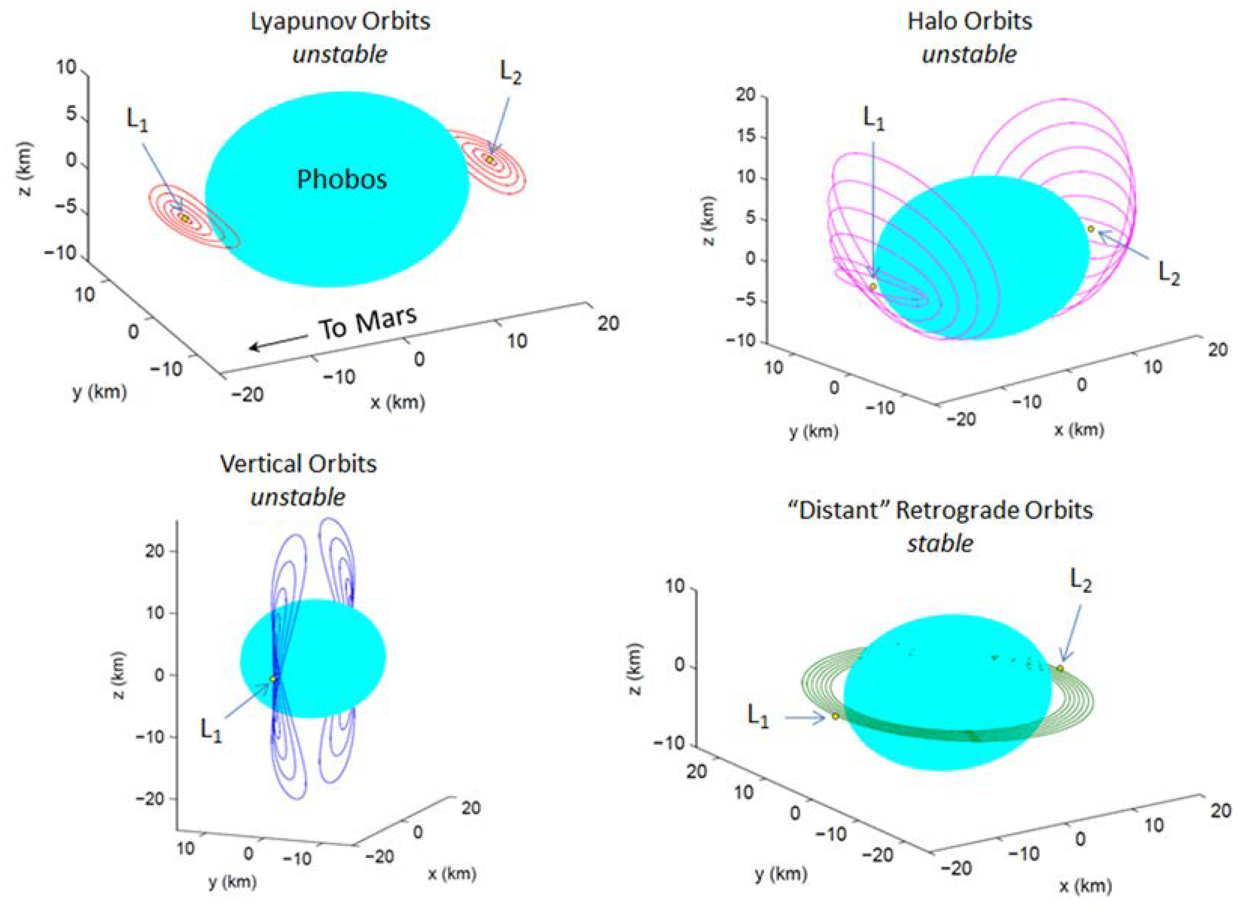
Figure 2.
Graphic representation of parameters [,] to optimize to generate a periodic DRO in the CR3BP rotating reference frame .
Figure 2.
Graphic representation of parameters [,] to optimize to generate a periodic DRO in the CR3BP rotating reference frame .
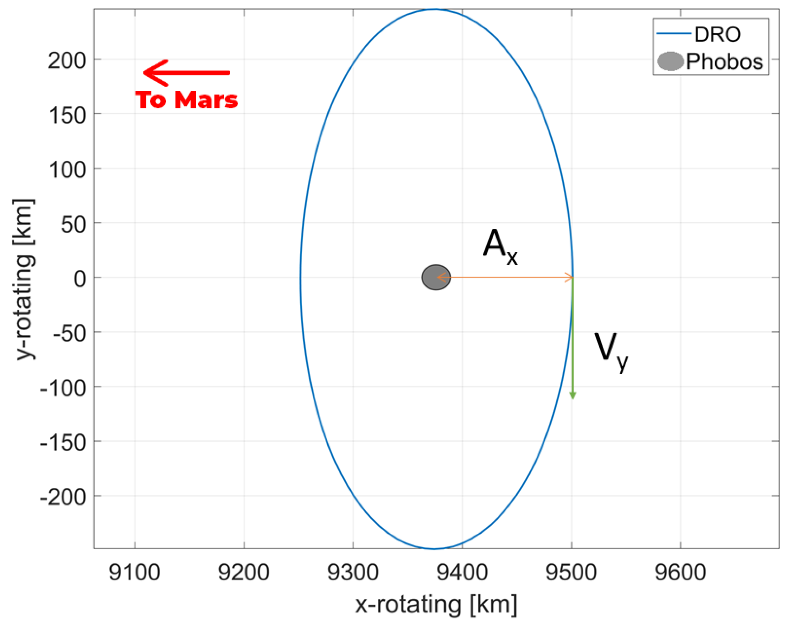
Figure 3.
Mars-Phobos DRO samples with Lagrange Points and for reference.
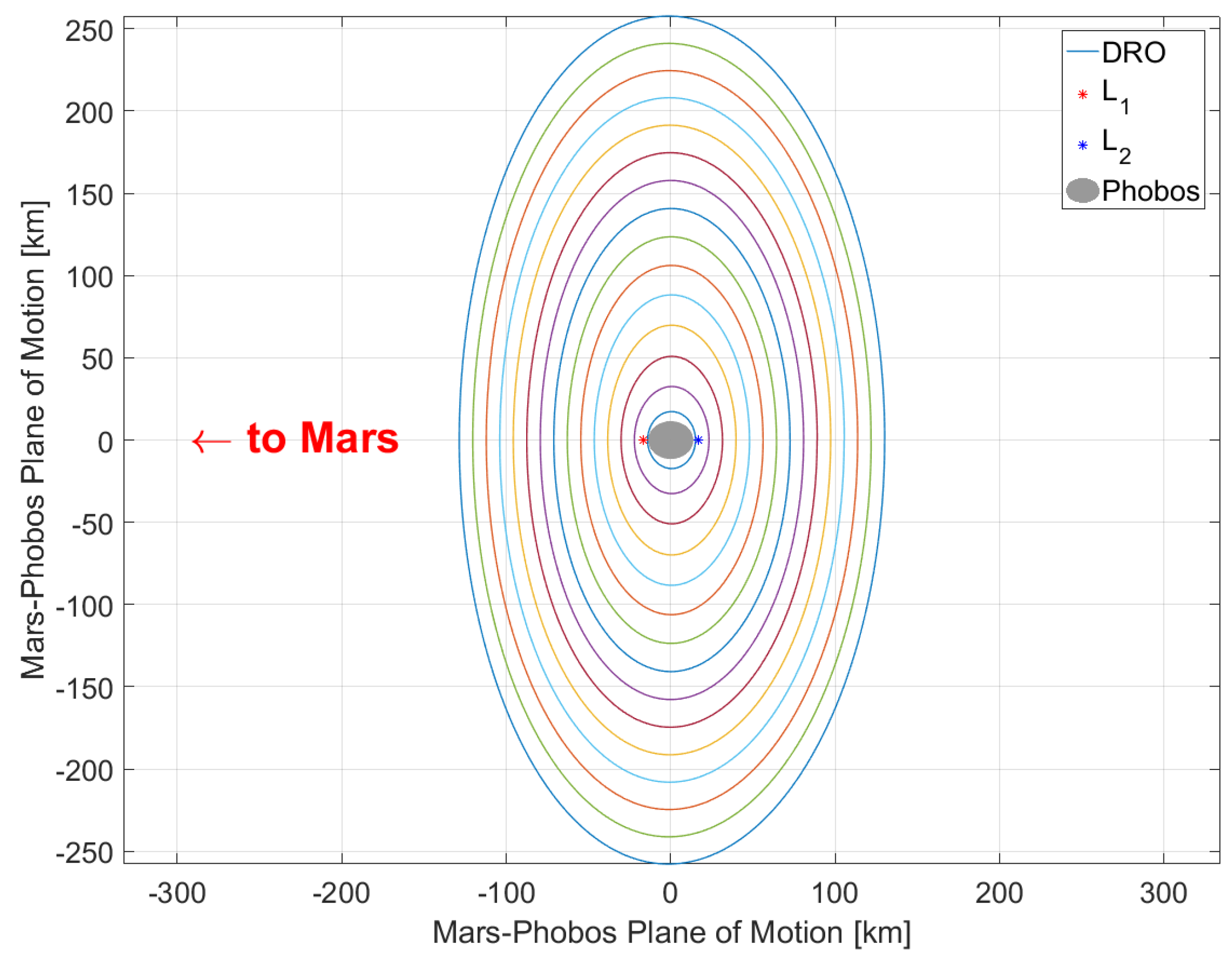
Figure 4.
Flow Chart for PSO algorithm.
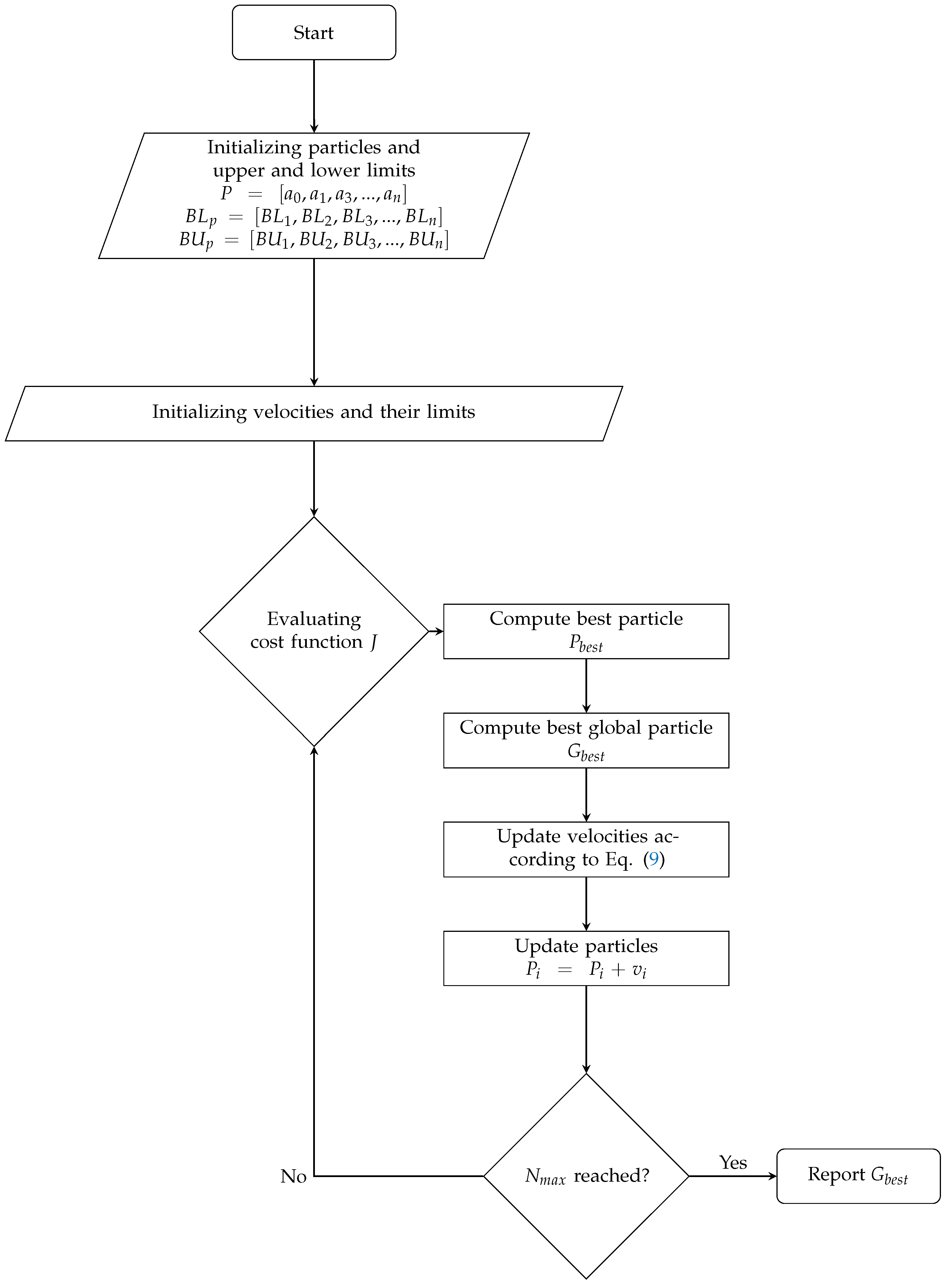
Figure 5.
Geometry of the restricted three-body problem.
Figure 6.
Mars-Phobos DRO for km resulting from the Particle Swarm Optimization.
Figure 7.
Cost Function J compared to Iteration Number for different DRO amplitudes.
Figure 8.
Graphic representation of parameters , and . These are the parameters to optimize in the landing trajectory analysis of this study.
Figure 8.
Graphic representation of parameters , and . These are the parameters to optimize in the landing trajectory analysis of this study.
Figure 9.
Phobos’ sector division and qualitative landing trajectories.
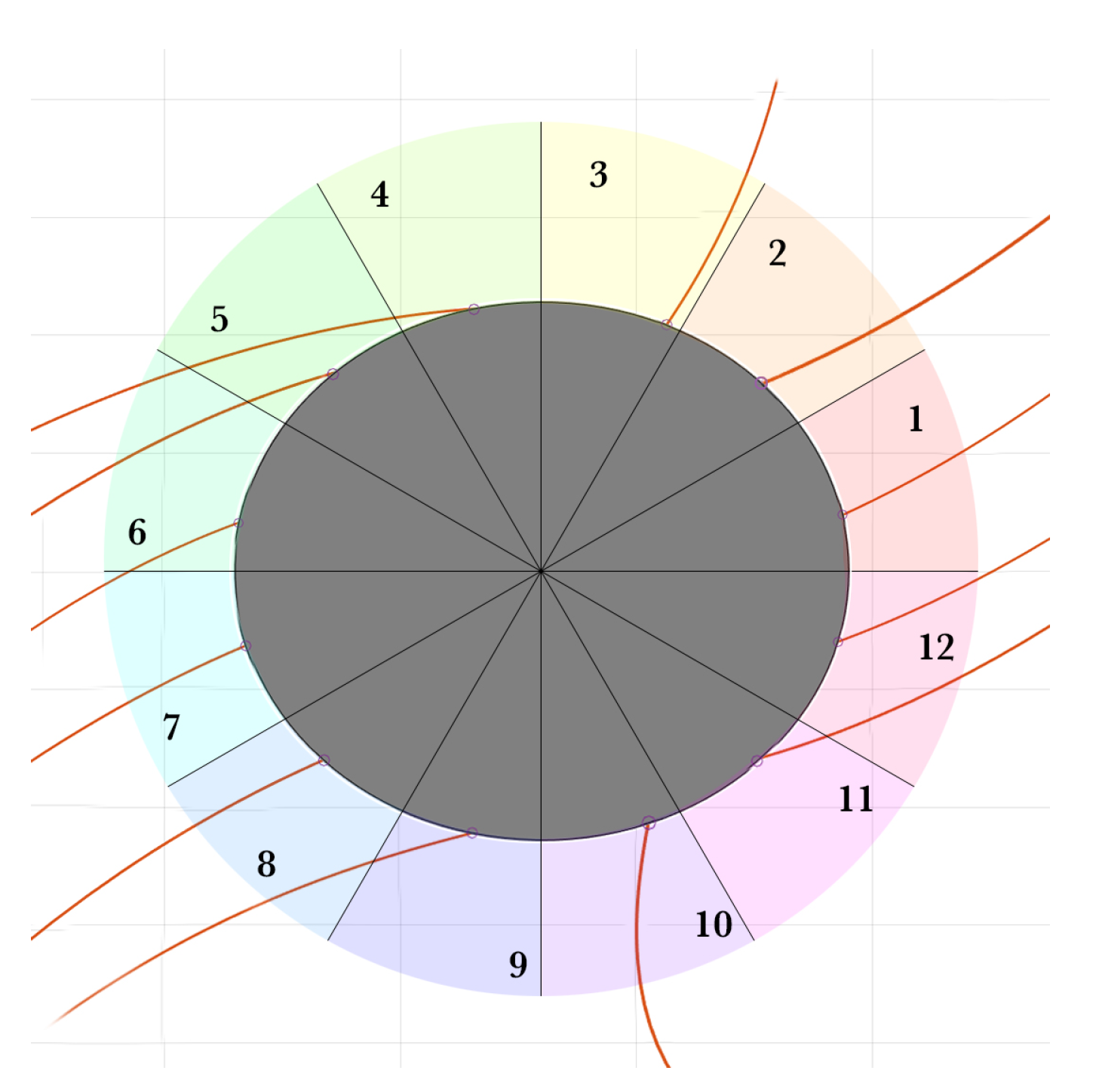
Figure 10.
Landing trajectories for each sector. Details are summarized in Table 7.
Figure 10.
Landing trajectories for each sector. Details are summarized in Table 7.
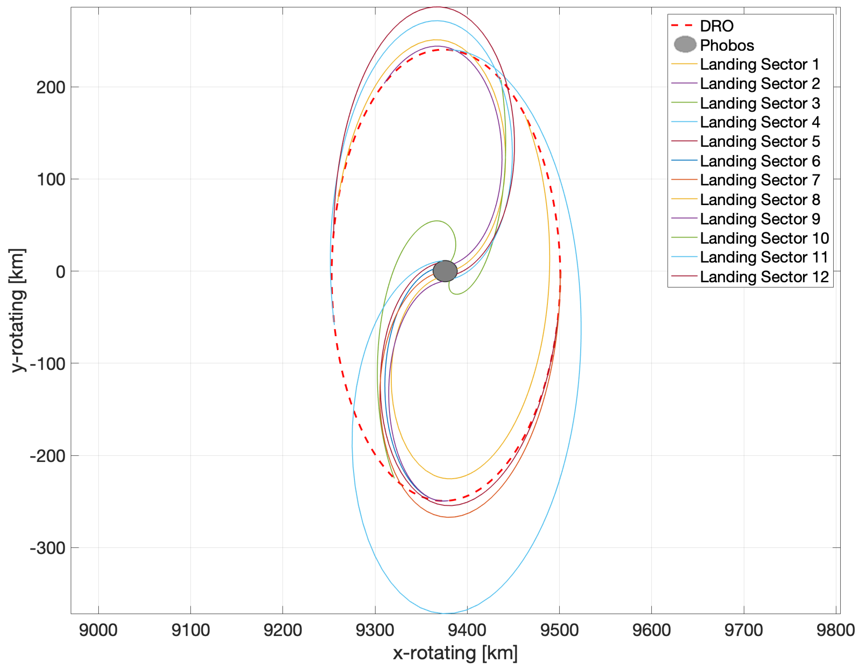
Table 3.
Computer system characteristics.
| Item | Description |
|---|---|
| Operating System | MacOS Big Sur Version 11.2.3 |
| Processor | 3.3 GHz Dual-Core Intel Core i7 |
| RAM | 16 GB 2133 MHz |
| MatLab version | R2020b Update 3 |
| System architecture | 64-bit operating system, x-64-based processor |
Table 4.
Boundary Values for Landing Optimization using PSO.
| Variable | Value | Description |
|---|---|---|
| () | 0 | Lower limit for (km/s) |
| () | Upper limit for (km/s) | |
| () | 0 | Lower limit for (rad) |
| () | Upper limit for (rad) | |
| () | 0 | Lower limit for (rad) |
| () | Upper limit for (rad) | |
| 200 | Maximum number of iterations | |
| 100 | Number of particles |
Table 5.
Initial values for Landing Trajectory Optimization
| Variable | Value | Description |
|---|---|---|
| (km) | Initial position of parking DRO |
|
| (km/s) | Orbit velocity at position |
|
| (s) | Orbital period |
Table 6.
Computation times for Landing Optimization Algorithm.
| Landing Location Sector | Computation time |
|---|---|
| 1 | 2 min, 56 s |
| 2 | 2 min, 21 s |
| 3 | 3 min, 20 s |
| 4 | 2 min, 17 s |
| 5 | 2 min, 42 s |
| 6 | 2 min, 15 s |
| 7 | 2 min, 56 s |
| 8 | 3 min, 17 s |
| 9 | 2 min, 21 s |
| 10 | 2 min, 19 s |
| 11 | 2 min, 53 s |
| 12 | 4 min, 8 s |
| Average | 2 min, 54 s |
Table 7.
Final results for Landing Optimization at one landing location for each sector.
| Landing Loc. Sector | Time of Flight | Total (m/s) | (°) | (°) |
|---|---|---|---|---|
| 1 | 4 hrs, 41 min | 27.35 | 246.10 | 147.14 |
| 2 | 3 hrs, 51 min | 29.24 | 205.53 | 108.16 |
| 3 | 5 hrs, 10 min | 31.02 | 347.27 | 256.35 |
| 4 | 7 hrs, 33 min | 32.42 | 101.32 | 89.22 |
| 5 | 4 hrs, 54 min | 27.27 | 88.41 | 337.07 |
| 6 | 3 hrs, 29 min | 32 | 0 | 270.49 |
| 7 | 5 hrs, 13 min | 27.41 | 100.38 | 0 |
| 8 | 6 hrs, 6 min | 28.72 | 154.32 | 62.75 |
| 9 | 3 hrs, 41 min | 31.93 | 0 | 270.84 |
| 10 | 4 hrs, 24 min | 31.34 | 168.82 | 73.85 |
| 11 | 5 hrs, 36 min | 27.66 | 260.27 | 204.36 |
| 12 | 5 hrs, 13 min | 30.25 | 209.12 | 161.04 |
| Average | 4 hrs, 59 min | 29.72 m/s |
Disclaimer/Publisher’s Note: The statements, opinions and data contained in all publications are solely those of the individual author(s) and contributor(s) and not of MDPI and/or the editor(s). MDPI and/or the editor(s) disclaim responsibility for any injury to people or property resulting from any ideas, methods, instructions or products referred to in the content. |
© 2023 by the authors. Licensee MDPI, Basel, Switzerland. This article is an open access article distributed under the terms and conditions of the Creative Commons Attribution (CC BY) license (https://creativecommons.org/licenses/by/4.0/).
Copyright: This open access article is published under a Creative Commons CC BY 4.0 license, which permit the free download, distribution, and reuse, provided that the author and preprint are cited in any reuse.


