
Submitted:
12 February 2025
Posted:
13 February 2025
You are already at the latest version
Abstract
Developing spacecraft for efficient aerocapture missions demands managing extreme aerothermal environments, precise controls, and atmospheric uncertainties. Successful designs must integrate vehicle airframe considerations with trajectory planning, adhering to launcher dimension constraints and ensuring robustness against atmospheric and insertion uncertainties. To advance robust multi-objective optimization in this field, the new framework is presented, designed to rapidly analyze and optimize non-thrusting, fixed angle-of-attack aerocapture-capable spacecraft and their trajectories. The framework employs a 3-degree-of-freedom atmospheric flight dynamics model incorporating planet-specific characteristics. Aerothermal effects are approximated using established Sutton-Graves, Tauber-Sutton, and Stephan-Boltzmann relations. The framework computes the resulting post-atmospheric pass orbit using an orbital element determination algorithm to estimate fuel requirements for orbital corrective maneuvers. A novel algorithm that consolidates multiple objective functions into a unified cost function is presented and demonstrated to achieve superior optima with computational efficiency compared to traditional multi-objective optimization approaches. Numerical examples demonstrate the methodology’s effectiveness and computational cost at optimizing Terrestrial and Martian Aerocapture maneuvers for minimum fuel, heat loads, peak heat transfers, and an overall optimal trajectory, including volumetric considerations.
Keywords:
aerocapture maneuver
; parameter optimization
; multi-objective optimization
; mission design and planning
1. Introduction
A critical step in planetary research is capturing a spacecraft from its hyperbolic trajectory to a closed orbit around the target planet. The traditional insertion burn method requires significant fuel allocation, reducing payload mass fraction. The aerocapture maneuver offers a solution that bypasses the need for large fuel fractions, potentially increasing payload capacity. Despite extensive study and optimization efforts, its implementation in interplanetary missions is yet to be realized due to spacecraft architecture difficulties and mission outcome sensitivity to minor, unpredictable uncertainties.
Recent optimization efforts in this field [1,2,3,4] have centered on the pursuit of efficient trans-atmospheric trajectories through meticulous manipulation of drag and lift forces to achieve an optimal aerocapture maneuver. Recent years have witnessed a push towards enhancing aerocapture technology through drag modulation (DM) techniques. These methods enable control over the spacecraft’s ballistic coefficient () by manipulating either the reference area or the drag coefficient () through continuous or discrete strategies, simplifying avionics and obviating the need for complex attitude control systems. However, certain technical challenges remain [5]. In contrast, with a history of successful missions, lift modulation relies on complex avionics algorithms and control systems for continuous bank angle modulation. Despite the complexities associated with this technique, it remains better understood and established than DM techniques. Optimal aerocapture problems have often overlooked the complex engineering intricacies inherent in effecting control over these parameters. Furthermore, the influence of aerodynamic control on the resulting captured orbit is limited, and its nature is highly dependent upon the spacecraft’s state at the atmospheric interface . Consequently, optimizing the atmospheric trajectory yields only incremental benefits to the overall mission, primarily impacting atmospheric phenomena such as heat loads.
Current optimization strategies face challenges due to highly nonlinear physics, requiring intricate nonlinear programming methods to address potential non-convexity. While Liu et al. [2] explored optimizing nonlinear, heavily constrained re-entry trajectories by reframing the nonlinear problem as a convex one, their approach compromises generalizability, limiting its applicability. Hongwei et al. [6] tackle the inherent non-linearity of the problem by reformulating it into a convex sub-problem. This reformulation enables the efficient resolution of the original problem through a sequence of convex optimization tasks. Nevertheless, this approach is also applied to the optimal guidance of the spacecraft during re-entry. Additionally, current strategies often employ multi-objective optimization (MOO) [1,2,3,4] for optimal re-entry trajectory problems, presenting numerical and decision-making challenges. MOO involves navigating a multi-dimensional objective space, resulting in trade-offs between objectives. The exploration of vast potential solutions and the non-convex and irregular Pareto front further complicates optimal solution searches. Selecting a single solution from a multitude of trade-offs involves considering subjective preferences, priorities, and uncertainty, requiring informed judgment, which can be challenging for algorithms due to ambiguous decision-making criteria. Moreover, the AMAT framework, developed by Girija et al. [7] based on previous work by Girija [8], offers a Python-based tool to assist in the design of re-entry vehicles. This framework is specifically geared towards facilitating trade-off analysis rather than optimizing the design process.
In light of these multifaceted challenges, we propose a novel framework, based around a new algorithm for the Determination of Aerocapture Successful Trajectories and Robust Optimization (D-ASTRO) algorithm. Developed within the MATLAB environment, D-ASTRO is an efficient and robust tool for rapidly analyzing and optimizing generic aerocapture missions. D-ASTRO’s unique capability lies in its ability to rapidly optimize non-thrusting, fixed angle-of-attack aerocapture-capable spacecraft and trajectories. By requiring only minimal aeroshell information and mission parameters, D-ASTRO employs a nonlinear, single-objective constrained optimization strategy to identify optimal values for the flight path angle () at the AI and the fixed ballistic coefficient () of the aeroshell.
This paper’s structure proceeds as follows: In Section 2, we outline the equations of motion and physics models employed by D-ASTRO. Section 3 introduces the concept of the aerocapture corridor. The optimization problem, along with novel objective functions and performance metrics, is discussed in Section 4. The novel methodology used to rapidly compute the aerocapture corridor rapidly is covered in Section 5 while Section 6 focuses on the Numerical implementation and pipeline of the algorithm. Finally, Section 7 presents the algorithm’s numerical stability and convergence properties applied to a typical Martian aerocapture mission test case, with computational considerations and performance of D-ASTRO explored in Section .
2. Equations of Motion and Physics Model
2.1. Atmospheric Flight Dynamics
This framework supports the preliminary design and optimization of aerocapture-capable spacecraft. At this stage, key geometric parameters such as the inertia matrix, center of mass, and center of pressure are undefined, limiting the analysis of rotational kinematics during re-entry. Consequently, D-ASTRO employs a three-degree-of-freedom (3-DOF) model, following the equations outlined by Kumar and Tewari [9]:
where r is the radial distance from the planet’s center to the vehicle, V is the planetocentric velocity, is the flight path angle, and are the longitude and latitude, respectively, and is the heading angle. Additionally, m denotes the spacecraft’s mass, L and D are the lift and drag forces, respectively, and and represent the planet’s gravitational parameter and rotational period, respectively.
Let the trajectory state in Equation (1) be . The initial condition of is assumed to be user-specified and coincident with the atmospheric interface (AI).
2.2. Aerodynamics Model
The aerodynamic model assumes the Mach independence principle, simplifying the determination of aerodynamic drag for hypersonic continuum flows, resulting in a single and that characterize the entire high-altitude trajectory. However, phenomena such as gas rarefaction at high altitudes can cause deviations from the Mach independence principle. To account for this, D-ASTRO allows users to input and as a function of Mach number, M, Reynolds number, , and Knudsen number, for greater accuracy, as described by Equations (2) and ().
where is the freestream density and is the reference area of the aeroshell
2.3. Aerothermal Model
To compute the heat flux, and heat load, Q, of the trajectory is a simplistic manner, the thermal model focuses on stagnation point aerothermal heating, as this is the expected peak heat transfer region of the aeroshell. Thus, the Sutton-Graves relation [10], Equation (4), approximates the convective stagnation point heating. Furthermore, D-ASTRO incorporates the Tauber-Sutton relations [11], Equation (), to account for radiative heat transfer, , in cases where re-entry speeds are moderately high.
where is the nose radius, k, C, a and m are atmospheric-specific constants, and is an empirically determined function that is also planet-specific.
In cases where wall temperature is a concern, radiative equilibrium approximates the equilibrium wall temperature, . Assuming an energy balance between total heating, , and re-radiative cooling, , calculated using the Stefan-Boltzmann law, Equation (7) is approximated by (Equation 8).
where is the emissivity and is the Boltzmann constant.
2.4. Atmospheric Model
A reliable atmospheric model is essential for accurately calculating the vehicle’s aerodynamic forces and aerothermal heating during the aerocapture maneuver. This report investigates Terrestrial and Martian atmospheres, highlighting their specific models below.
2.4.1. Earth Atmospheric Model
Given the high altitude characteristic of aerocapture trajectories, the U.S. standard atmospheric model [12] was deemed inadequate. Instead, the Earth atmosphere model proposed by NASA [13] (Equation (8)) will be utilized as an initial approximation. As discussed in Section 3, the robustness of an aerocapture corridor hinges on uncertainties in atmospheric properties, particularly density. More reliable atmospheric models exist that incorporate seasonal and global positioning variations in atmospheric quantities, like NASA’s Earth Global Reference Atmospheric Model (Earth-GRAM) [14] and COSPAR International Reference Atmosphere (CIRA) model [15].
To account for atmospheric perturbations, the research by Leslie and Justus [14] is used, indicating a maximum density fluctuation of 25% for ±3 standard deviations in the 0-80 altitude range. As Terrestrial aerocapture maneuvers are not the main focus of this study, ±30% fluctuations in density corresponding to 3 standard deviation perturbations are assumed to approximate uncertainties in density.
which is applicable for .
2.4.2. Mars Atmospheric Model
Mars-GRAM [16] was employed to generate atmospheric data for Martian aerocapture maneuvers. A simplified table was generated from the extensive data available in the Mars-GRAM database, encompassing atmospheric variations concerning seasons, latitude and longitude positions, and numerous other variables. This table is based on a yearly average of equatorial properties at zero longitude. Additionally, a statistical analysis was conducted to ascertain an accurate variation of atmospheric properties for , which encompasses 99.73% of cases.
2.5. Orbital Element Determination
Determining orbital elements is crucial for characterizing a spacecraft’s orbit after an atmospheric pass. Identifying the nature of this orbit is essential to assess the success of the aerocapture maneuver. Additionally, these elements play a vital role in the proposed optimization strategy, as they will dictate the required fuel for corrective maneuvers. D-ASTRO employs an orbital determination algorithm based on the method proposed by Curtis [17], summarized in the pseudo-code shown in Algorithm , to compute the orbital elements.
3. Aerocapture Corridor
Without employing lift or drag modulation, the flight path angle at AI and are the primary factors governing the vehicle dynamics during the atmospheric pass, thus determining the success of the aerocapture maneuver. The aerocapture corridor defines the range of and values that result in a successful maneuver. The lower limit occurs when excessive drag causes the spacecraft to collide with the surface. In contrast, the upper limit occurs when insufficient drag causes the vehicle to remain in a hyperbolic orbit. The lower limit is easily computed when the altitude reaches zero at any point in the trajectory. The spacecraft’s post-pass orbital eccentricity e determines the upper limit, where indicates a closed orbit.
Figure 1.
Example of Martian aerocapture corridors with post-atmospheric pass orbital eccentricity contours: (a) Ballistic re-entry profile, . (b) Lifted re-entry profile,
Figure 1.
Example of Martian aerocapture corridors with post-atmospheric pass orbital eccentricity contours: (a) Ballistic re-entry profile, . (b) Lifted re-entry profile,
Figure compares the aerocapture corridors for ballistic and lifting re-entry profiles of a spacecraft approaching Mars with a hyperbolic excess velocity, , of 3.5 . The maneuver’s success is represented by green hashing in Figure . These contours are depicted in the figures. These contours illustrate the intricate relationship among , , and the lift-to-drag ratio necessary for successful maneuvers. A lifting re-entry profile provides a more favorable corridor, reducing sensitivity to precise insertion attitudes. While D-ASTRO supports various re-entry profiles, this study focuses on non-zero profiles for Martian aerocapture, utilizing a fixed value of 0.2, consistent with established norms for Martian re-entry vehicles [18].
Uncertainties in atmospheric properties significantly influence the width of the aerocapture corridor. Variations in atmospheric density lead to changes in drag forces, causing the spacecraft to dissipate energy differently than expected. Near the aerocapture boundaries, even minor density fluctuations can result in maneuver failure, leading to either a hyperbolic orbit or surface collision. Two corridors are computed to establish a robust corridor: one with reduced atmospheric density and another with increased density. The `robust’ aerocapture corridor represents the intersection of these two, resulting in a narrowed corridor. These corridors are illustrated in Figure 2, depicting Terrestrial and Martian corridors for various inbound , where the green and yellow regions represent the robust and non-robust corridors.
4. Optimal Aerocapture Maneuver via Parameter Optimization
Multiple approaches can be taken to optimize an aerocapture trajectory. However, we focus on the optimization of design parameters and which yield a successful aerocapture trajectory. Determining these two parameters allows mission planners to identify the most suitable interplanetary orbit and structural design of the heat shield to ensure a successful and optimal trajectory.
4.1. Formulation of Optimization Problem
The optimal aerocapture corridor problem is a constrained nonlinear optimization problem of the
form:
where f represents the objective function, and and are functions of that define the upper and lower boundaries of the aerocapture corridor. The vector comprises selected performance indices.
Insertion inaccuracies during aerocapture missions can arise from accumulating minor guidance errors during the interplanetary trajectory. This leads to significant deviations from the intended atmospheric insertion coordinates. Deviating from the intended leads to different atmospheric trajectories, impacting the aerocapture maneuver’s optimality and sometimes the success. To account for this, an expected insertion inaccuracy is incorporated as , which narrows the aerocapture corridor to ensure mission success is robust to insertion inaccuracies.
4.2. Performance Indices
This section introduces a series of typically used performance metrics for re-entry trajectories.
4.2.1. Thermal Environment
The corresponding aerocapture trajectory is computed for every candidate point, and the profile is available. Hence, is computed by locating the maximum value in the profile and Q by using Equation (10).
where is the total duration of the atmospheric flight.
4.2.2. Volumetric Constraints
To address fairing constraints and current technological limitations, this optimization process aims to minimize the volume of the aeroshell by reducing the “equivalent axisymmetric aeroshell radius” , , computed by rearranging Equation (11). This metric is preferred because it can represent any aeroshell configuration, from axisymmetric to complex high lift-to-drag designs, as long as and are known.
4.2.3. Orbital Corrective Maneuvers
represents the fuel needed to adjust the post-atmospheric pass orbit to the predetermined target orbit. In reality, each candidate trajectory will have its unique optimal orbital corrective maneuver composed of complex transfers. To simplify comparisons between all candidate trajectories, trivial orbit transfers are used. These include two-impulse Hohmann transfers to raise the orbit’s periapsis and match the desired target orbital eccentricity. In addition, a plane change burn at the apoapsis is assumed to match the target orbital inclination. The required can be computed using Equation (12).
where a is the semi-major axis of the orbit and subscripts `i’ and `t’ , denote the quantity evaluated at the post-atmospheric pass orbit (determined at AE) and the target operational orbit, respectively.
4.3. Single-Objective Function Optimization
This paper considers two formulations of optimization Problem Section 4.1. The first strategy is the most widely employed multi-objective optimization (MOO), where , and a novel single objective optimization formulation is presented, where .
MOO is the preferred approach for re-entry trajectory optimization, addressing problems with multiple conflicting criteria that cannot be combined into a single objective. However, MOO methods face challenges, including non-unique optimal solutions and subjective decision-making. Additionally, achieving both convergence and diversity—how close and spread the candidate solutions are relative to the Pareto front— is complex. Consequently, a new optimization problem may need to be formulated to address these issues and improve the performance of the MOO process.
This paper introduces a novel optimization problem that combines all the discussed performance indices into a single objective function. This enables the use of traditional gradient descent (GD) methods to solve the problem. The proposed objective function utilizes the weighted least squares (WLS) approach and is presented below.
where w is the weight vector that includes the biasses of each performance index, and the definition of follows.
Unlike MOO, the proposed Single-Objective Optimization (SOO) problem requires feature scaling due to significant differences in magnitudes among the performance indices. Specifically, Q is typically 5 to 7 orders of magnitude higher than and . To avoid biasing the results towards minimizing the performance index with the most significant magnitude, feature scaling is employed. The normalization technique rescales the performance indices between 0 and 1, as shown in Equation (15).
where and represent the upper and lower bounds of property . To perform normalization accurately, it is essential to know the range of possible values that each feature can take. However, computing this range is not trivial, and an approximate procedure can be employed, which will be explained in Section 6.
5. Approximating Aerocapture Corridor Boundaries
The primary challenge in aerocapture optimization lies in handling the nonlinear constraints introduced by and in Problem P1. Current optimization techniques necessitate computing and at each internal candidate point, significantly increasing execution time despite efficient search algorithms. This is quantitatively characterized in Section .
Multiple aerocapture corridors for Martian and Terrestrial missions with various hyperbolic approach orbits were analyzed. Figure 2 displays three examined corridors, with the upper boundary exhibiting an exponential trend across all cases, while the lower boundary differs from this trend in some scenarios. This discrepancy is imparted by the differing atmospheric structures of the planets at low altitudes. Several candidate fundamental functions were considered to rapidly map to and , including exponential and polynomial curves.
Initial testing revealed limitations of a primary exponential curve ( in Equation (16), leading to the adoption of a second-degree exponential fit (), significantly enhancing predictive accuracy with error bounded by and for Terrestrial and Martian aerocaptures respectively. Additionally, sixth-degree polynomial curves were examined due to the potential flat nature of some boundaries. As illustrated by Figure 3, the polynomial curves resulted in excellent predictive capabilities, exceeding the former’s accuracy.
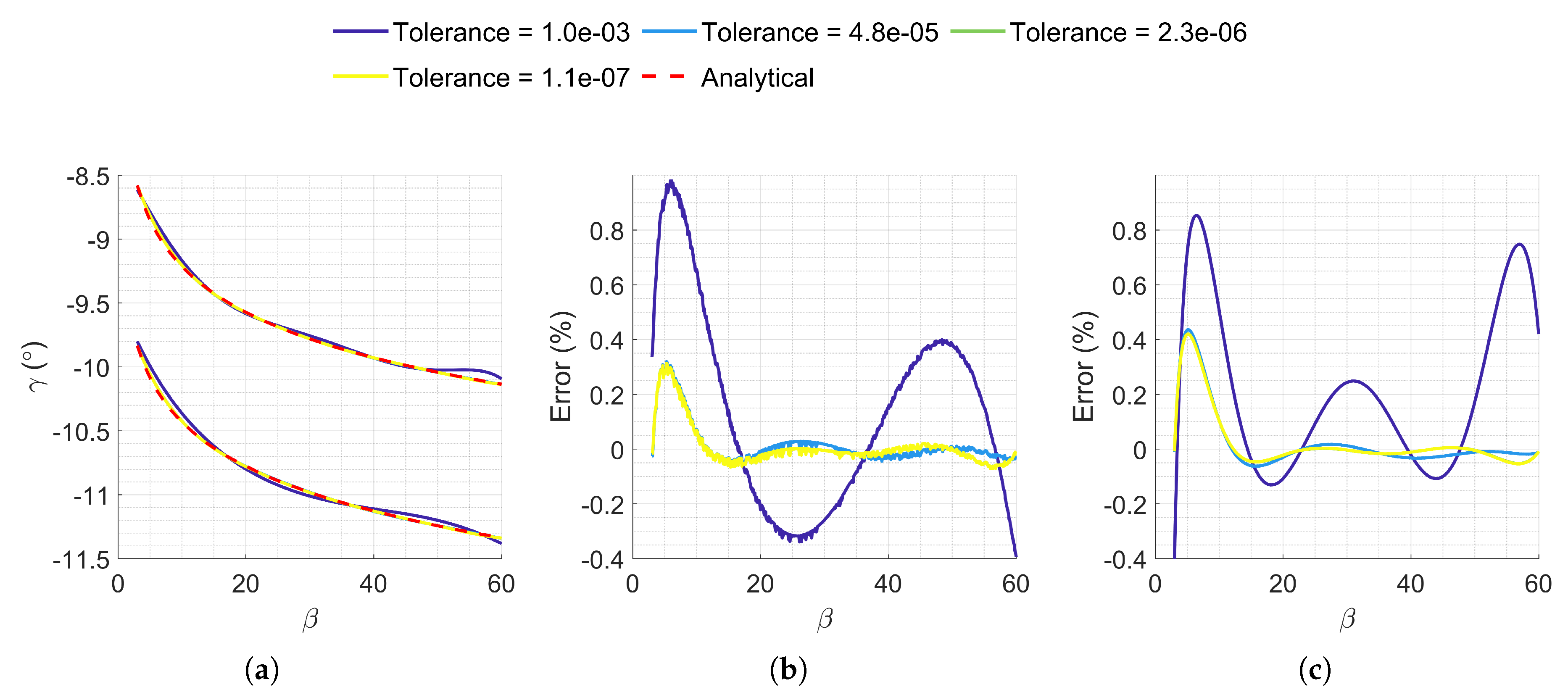
Exploration into the minimum number of points required for accurate fitting demonstrated that the accuracy of the fits was very sensitive to the selected fitting points. Randomly selecting seven points within the interest range demonstrated poor fit accuracy, as illustrated by Figure A1. However, when the fitting points were evenly distributed across the range, both fits exhibited increased accuracy with fewer fitting points. Specifically, fitting the sixth-degree polynomial with seven linearly spaced points proved to capture boundaries accurately, showcasing superior capabilities in approximating flat boundaries, resulting in approximations within and for Terrestrial and Martian maneuvers, respectively. Figure 3 illustrates the error between the actual boundary and the proposed fits, comparing the second-degree exponential fit with the sixth-degree polynomial fit, both fitted with 7 linearly spaced points.
6. The D-ASTRO Framework
The novelty of D-ASTRO lies in its pre-optimization phase, where complex physics are efficiently analyzed to enhance the robustness and speed of the optimization. The key aspects of this stage are detailed in the following sections.
6.1. Computation of Normalization Quantities
As discussed in Section 4.3, computing the extremal values of the performance metrics in is crucial for casting the optimization problem into SOO form. We investigate which and values may achieve these targets.
For volumetric constraints, the bounds are easily computed based on , with maximum and minimum volumes corresponding to the lower and upper limits of , respectively. Thermal metrics, such as , increase with deeper atmospheric entries, so reaches its maximum at the lower corridor boundary and upper limit, while the minimum occurs at the upper corridor boundary and lower limit. The same applies to Q, which is maximized for deeper entries. Determining the bounds of is more complex, as post-atmospheric trajectory eccentricities can span from 0 to 1 within the aerocapture corridor. If circularization and plane change maneuvers are neglected, . Hence, we assign , while depends on the operational orbit and requires assessment across the .
This analysis focuses on identifying the maximum and minimum values within the corridor. While the optimizer can explore and values beyond those used for normalization, this discrepancy does not significantly impact the process. Normalization ensures that values remain on a similar scale, with values exceeding the estimated maximum normalized above 1 and smaller values becoming negative. However, the non-linear constraints and enforce candidate points within the corridor, mitigating this issue.
6.2. Computation of Polynomial Fits
A key step is generating polynomial fits to approximate the corridor boundaries. As described in Section 5, this requires computing and at seven evenly spaced values to capture boundary dynamics accurately. This allows the normalization metric search to integrate with the boundary value computations for curve fitting. The complete D-ASTRO framework is detailed in the next section.
6.3. The Framework
A user-specified range is sampled with seven linearly spaced points, including the upper and lower limits. From this analysis, values for are computed, while the remaining points focus on and corridor boundaries and , with set to zero. A binary search determines ’s lower and upper boundary values at each , which are then fitted with a sixth-order polynomial. After computing normalization quantities and polynomial fits, MATLAB’s fmincon optimizer is used, employing sequential quadratic programming with an active set strategy, as described by Gill et al. [19]. The robust aerocapture corridor and polynomial fits are shown in Figure 4, with the normalization values listed in Table 1.
7. Results and Analysis
A Martian aerocapture mission is considered to assess the robustness and convergence properties of the proposed optimization strategy. The Martian atmosphere is modeled using data from Mars Global Reference Atmospheric Model 2010 (Mars GRAM 2010) [16] (an engineering-level atmospheric tool developed for mission design applications). D-ASTRO requires multiple input parameters, including spacecraft preliminary properties, interplanetary insertion trajectory, and target operational orbit. These input quantities are provided in Table 2 and Table 3.
7.1. Dependencies on Solver Initial Conditions
The optimization algorithm was subjected to various initial conditions to assess its convergence properties. A bias vector assigning equal importance to all performance indices (denoted as ) was employed for this examination. The range of considered initial conditions comprised extreme and random values both within and outside the aerocapture corridor, with some having limited physical meaning. Table 4 provides detailed information on the initial conditions used ( and ).
In Figure 5, level lines of the cost function are depicted within and around the aerocapture corridor. The region delineated by magenta solid lines represents the aerocapture corridor, defined by the novel polynomial fit approach discussed in Section 6. The figure illustrates that the novel objective function formulation is well-suited for gradient descent (GD) algorithms, as it has no visible sharp discontinuities. Notably, areas where aerocapture fails, such as surface collisions in the lower left corner of the figure, incur high costs, expediting solution convergence.
Based on Table 4 and Figure 5, the problem’s minimum is near , though further investigation is needed to resolve discrepancies in the suggested optima and validate trajectory feasibility. While Case 2 indicates a slightly different optimal point (explored further in Section 7.2, the algorithm consistently converges to the global minimum, even with initial conditions lacking physical significance (e.g., Cases 1, 3, and 4). The strong convergence properties of D-ASTRO are further demonstrated by the similarity in trajectory profiles shown in Figure 6.
7.2. Minimum Fuel Mission Design
The adoption of an aerocapture maneuver is often motivated by a desire to minimize fuel requirements to achieve a desired operational orbit. The minimum fuel trajectory for the proposed case study can be identified by selecting . The same initial conditions as the previous section are studied to assess convergence properties. Additionally, various target semi-major axis values, specifically , , and , are analyzed to explore the behavior of the optimality valley introduced earlier.
As illustrated by the () cost contours in Figure 7 and the information in Table 5, this optimization problem yields optima that are scattered over a broader range. However, it is crucial not to interpret this as a sign of poor convergence of D-ASTRO’s optimizer. Instead, understanding the underlying physics and formulation of the optimization problem is essential to justify this apparent discrepancy.
Figure 7 illustrates the presence of a low-cost valley in the cost function, directing the global minimum along a specific direction. This flat valley is the reason behind the discrepancies in this scenario, with some minor discrepancies in the overall optimal trajectory. As shown in Figure 5 and Table 4, the optimum for Case 2 slightly deviates from other test cases but results in identical cost (accurate to four decimal places) as Cases 1 and 5. Although the low valley affects the minimum fuel mission design more, its impact on the optimal design with multiple metrics is minimal, ensuring good local agreement in the suggested optima.
The valley-like structure of the cost function characterizes a typical aerocapture corridor, with the trough’s vertical position determined by the target a. Smaller values require deeper atmospheric entries, shifting the valley downward, while larger values lead to shallower entries, moving it upward. The valley’s convex structure arises because one side requires increasing orbital energy due to excessive energy depletion, while the other side requires decreasing energy due to insufficient depletion. The valley in does not span the entire range; the increase in cost at low is linked to plane change maneuvers. Figure 8 illustrated the contours without considering these maneuvers, revealing the anticipated valley that spans the entire range. The evolution of plane changes result from the forces acting on the spacecraft during atmospheric entry, which do not align with the orbital plane, thereby altering the inclination of the orbit’s plane.
To enhance convergence and mitigate the impact on other cases, the cost function for must be revised. Comparing contours in Figure 8 and Figure 7a shows that including significantly increases fuel requirement. Applying feature standardization to the total flattens the valley as , causing to dominate the problem. To address this, a potential solution is to decompose the into two components and apply separate standardizations.
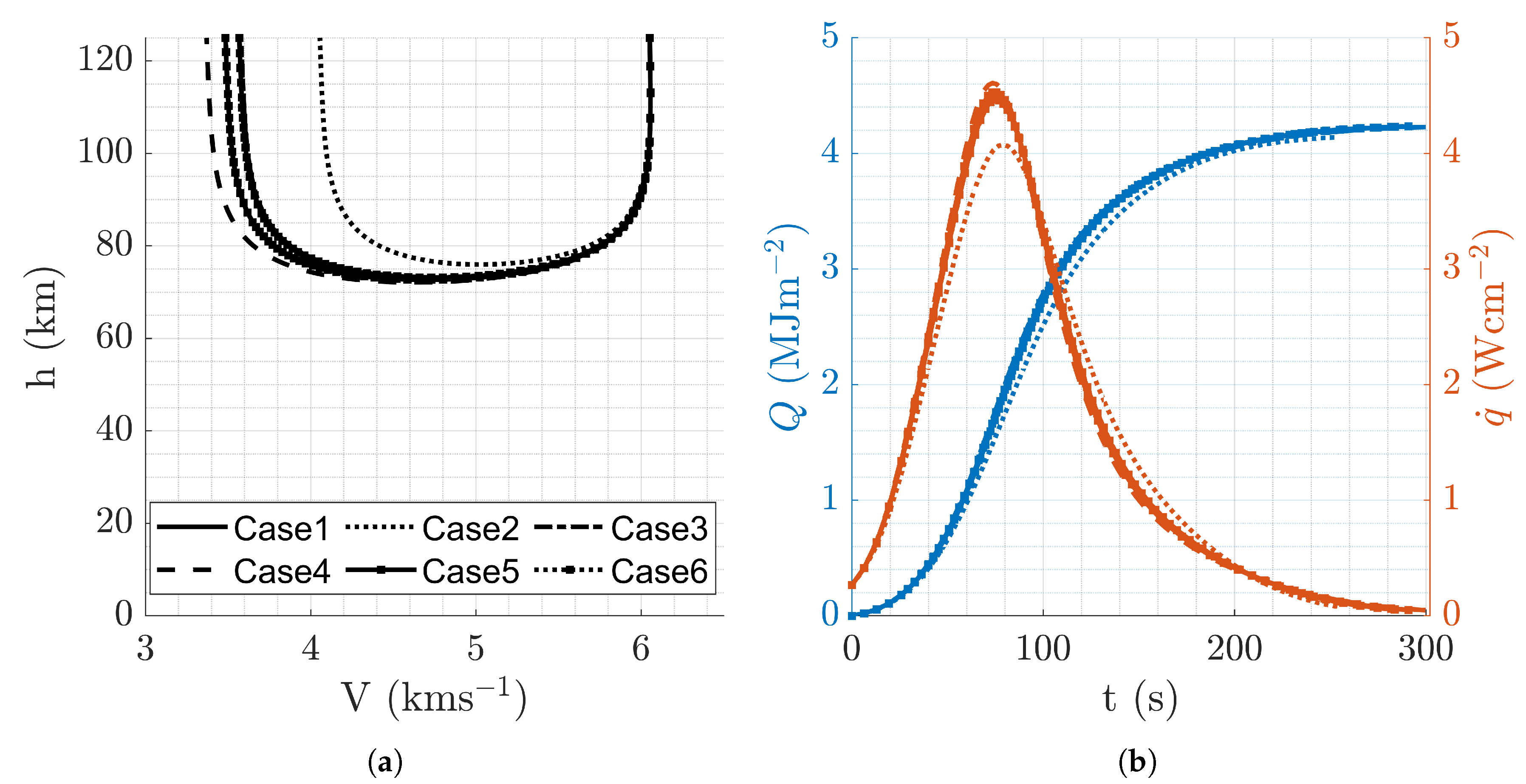
Figure 9 depicts the optimal trajectory profiles. The extensive variation in both and results in a multitude of trajectories. It is crucial to emphasize that despite discrepancies in the h-v profiles shown in Figure 9a, they all converge to a similar velocity (V) at the atmospheric exit, thereby leading to approximately comparable values of . As anticipated, thermal quantities exhibit significant differences across all trajectories, reflecting the lack of assigned importance to these features in the optimization process.
7.3. Minimum Heat Load Mission Design
Ensuring mission success during re-entry requires equipping the spacecraft with a suitably robust TPS. By minimizing the heat load experienced during the atmospheric trajectory, the TPS can be made more lightweight, allowing for an increased payload mass fraction.
As outlined by Equation (10), calculating stagnation point heat loads requires complete trajectory knowledge. In practice, researchers often use Equation (17) for simplified heat load estimations during Entry, Descent, and Landing (EDL), based only on parameters like and at AI. Utilizing the Sutton-Graves model for and an exponential atmospheric model, Allen and Eggers [20] formulated the complete expression, suggesting that heat load can be reduced by minimizing and maximizing . This approach is later explored as a substitute for the current Q cost function for aerocapture missions.
Figure 10 illustrates the exploration of multiple initial conditions aimed at determining the optimal trajectory with the minimum heat load, revealing partially anticipated trends. Table 6 details the outcomes of the explored cases. All cases suggest values near the lower limit of feasible , consistent with Equation (17). However, only Case 1 aligns with the minimum of Q predicted by Equation (17), with at the lower boundary of feasibility, while other cases show near the upper boundary.
To investigate the disparity between the anticipated minimum of Equation (17) and the complete trajectory analysis, both heat loads are normalized with respect to their corresponding minima and maxima and illustrated in Figure 11. This figure reveals differences in the contours of Q, particularly in the slopes with respect to ). The approximate expression in Equation (17) incorrectly suggests that increments on Q with , whereas the complete trajectory analysis shows the opposite trend . This discrepancy stems from the assumption of an EDL trajectory made by Allen and Eggers [20].
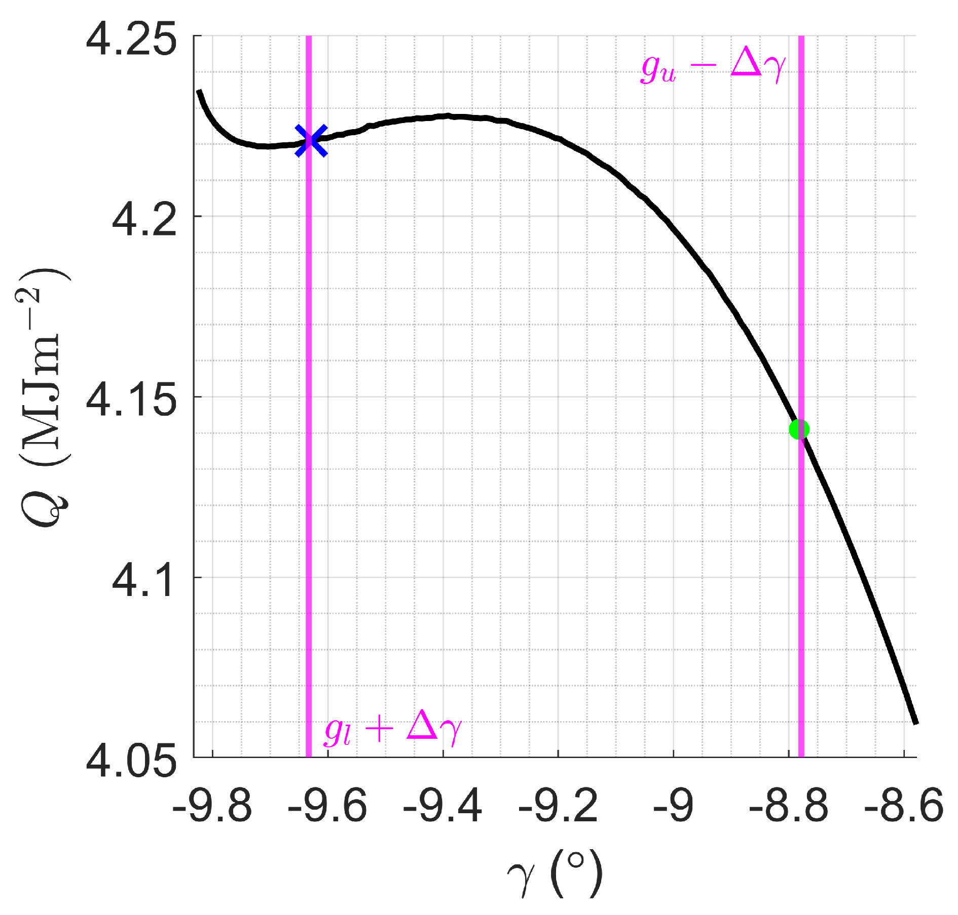
Optimizing for minimum Q highlighted the importance of the optimizer’s step tolerance in D-ASTRO robustness. Initially, fmincon’s default convergence criteria yielded reliable and consistent results, as demonstrated in Figure 5and Figure 7, and later shown in Figure 13. However, minimizing Q initially showed significant variations in due to the flat nature of the normalized Q () in the direction, with varying only slightly at the leftmost region of the corridor, of the order of . This was mitigated by reducing the function and step tolerance of the solver, causing D-ASTRO to identify the global minimum consistently, and in Case 1, a local minimum coincident with the feasibility boundary (see Figure A4). However, local minima can be avoided by selecting a reasonable initial condition. The decrement tolerance only benefits the convergence properties of the minimal Q trajectory, hindering the other problems with no changes in optimal trajectory for the other test cases. The resulting optimal trajectory profiles are shown in Figure 12, where the difference between the global and local minima trajectories can be seen.
7.4. Minimum Peak Heat transfer trajectory
Similar to the parameter Q discussed earlier, the peak heat transfer rate plays a crucial role in determining the design specifications of the TPS. This metric undergoes an independent optimization process to validate the underlying physics principles and the cost function employed.
The minimization of peak heat transfer demonstrates strong convergence properties, as shown in Figure 13 and Table 7, where multiple initial points converge to the same optima. The variation in convergence quality between Q and arises from the latter’s greater sensitivity to , illustrated by curved contours in Figure 13 versus the quasi-vertical contours of Figure 10. Figure 14 shows indistinguishable trajectory profiles, highlighting the optimizer’s excellent convergence
The results presented in Table 7 align with established expectations that smaller values of lead to reduced . However, the practical implementation of this solution is limited, as corresponds to an unfeasibly small value for a realistic mission as unprecedented aeroshell surface areas (A) would be required to achieve this . However, by introducing volumetric considerations in the optimization (non-zero first entry of ) will lead to more realistic . The resulting optimal points of combining thermal loads and volumetric considerations are illustrated in Table 9, where and are considered.
7.5. Direct Comparison with MOO
This section compares D-ASTRO with a basic MOO algorithm using MATLAB’s fgoalattain optimizer. Multiple Initial conditions are again tested to evaluate the solver’s convergence dynamics and stability. Figure 15 shows the convergence dynamics of both approaches, revealing significant disagreement in optimal solutions. Table 8 presents additional comparison, incorporating data from Table 4.
The subjective decision-making bias of MOO strategies is disregarded as the primary cause behind the disagreement between D-ASTRO and MOO results. A wide range of initial conditions consistently converge to one of two possible optima, corresponding to a local and global minimum. This is evident in Table 8, which shows reductions in , Q, and without compromising other performance metrics for Cases 4 and 5 when compared to other, similar to the local optima in the Q cost function (Figure A4). It is also worth noting that the optimization problem may not be ill-conditioned despite the absence of metric regularization in the MOO strategy, as the MOO optimization conducted with and without D-ASTRO’s normalization technique yielded identical results.
Further analysis revealed that the MOO strategy prioritized the optimization of Q and over and . As the MOO strategy suggested identical results for normalized and raw metrics, the discrepancy does not stem from dissimilar metric magnitudes but from the individual convergence dynamics of the metrics. As illustrated by Figure 10 and Figure 13, the heat load and peak heating rate cost functions exhibit a strong convex behavior in the direction, facilitating rapid convergence of GD algorithms to the leftmost regions. In contrast, the volumetric consideration cost function experiences an inverse proportionality to , leading to rapid convergence to the rightmost regions. Finally, the cost function experiences a convex-like behavior in the direction, causing the optimality valley explored in Section 7.2.
The dynamics of these metrics indicate three convergence behaviors: one toward the left region of the corridor, another toward the rightmost regions, and a third toward the corridor’s center. We conclude that the MOO optimizer is attempting to globally optimize Q and at the expense of . To later find the optimal in regions where Q and are quasi-globally optimal, as has relatively low cost over the entire range.
For completeness, all optimal trajectory profiles presented in this paper are illustrated in Figure 17 to aid the comparison between the different optima.
8. Computational Performance and Considerations of D-ASTRO
Section 7 demonstrated the superior convergence properties of D-ASTRO over conventional MOO strategies. This section examines the computational performance and considerations within the D-ASTRO framework. The analysis is divided into two parts: the first addresses the computational costs and considerations of the binary search algorithm used to compute the robust aerocapture corridor; the second evaluates the performance of the optimization process.
8.1. Dependency of Corridor fits on Binary Search Tolerance
To balance accuracy and computational efficiency, a study is conducted to analyze how the accuracy of the computed corridor boundaries varies with different tolerance levels. To evaluate this, we compute the robust coarse aerocapture corridor depicted in Figure 4 using varying binary search tolerances. The overall accuracy of the resulting polynomial fits is assessed by calculating the Euclidean L-2 norm between actual corridor boundaries, computed from a finely discretized aerocapture corridor (570 points), and those computed using the fits. Figure A5 illustrates the evolution of polynomial fit accuracy for both lower and upper corridor boundaries over the considered range. Additionally, Figure 18 presents the cumulative accuracy via the Euclidean L-2 norm approach and the execution time of the corridor, examining Martian and Terrestrial aerocapture maneuvers. This figure shows that the Euclidean norm reaches a plateau at a tolerance of approximately in both scenarios, indicating that more accurate fits are not achievable with a further decrement in tolerance. Hence, for expedited solutions of D-ASTRO, a binary search tolerance of is selected as the optimal balance between computational efficiency and accuracy. For the selected tolerance level, 31 trajectory simulations are required to compute and , with the number of simulations being unaffected by the chosen .
8.2. Execution Time of Optimizers
To evaluate the optimizers’ performance, 10 iterations of the optimization process were conducted using a consistent initial guess ( and ) to minimize execution timing outliers. Various weightings () were also considered to further explore the convergence properties of MOO and D-ASTRO, highlighting the challenges of the multi-objective approach in optimizing these problems. Table 9 presents the execution time, number of function calls, time per function call, and the suggested optima for both methods. This table indicates a significant dependency of execution time on the weight vector and optimization strategy employed. However, the time required per function call is roughly consistent across all cases, with the MOO function requiring marginally less time than D-ASTRO’s. This difference arises from the distinct optimizers used, as fgoalattain and fmincon are fundamentally different algorithms.
IIn general, D-ASTRO converges more quickly and with fewer iterations to the global optimum compared to the MOO strategy, except in the case where case. Under this condition, D-ASTRO requires more time but yields a solution that reflects a more balanced trade-off among all metrics, in contrast to the MOO strategy, which prioritizes Q and .
Comparing rows 3 and 4 reveals that different weightings do not impact the solution provided by MOO, whereas they clearly affect D-ASTRO’s solution. This behavior was consistent across multiple initial guesses and weightings. The only modification that enabled the MOO solution to depend on the weight vector was performing feature regularization. These findings underscore the superior capabilities of the D-ASTRO strategy over the multi-objective approach.

Table 9.
Computational Performance and Suggested Optima of D-ASTRO and MOO strategies with
and for Martian test case.
Table 9.
Computational Performance and Suggested Optima of D-ASTRO and MOO strategies with
and for Martian test case.
| weights | Strategy | Execution time (s) | Function counts | Time per function call (ms) | ||
|---|---|---|---|---|---|---|
| D-ASTRO | 1.889 | 1820 | 10.381 | 13.23 | -9.765 | |
| MOO | 0.381 | 360 | 9.979 | 3.03 | -9.638 | |
| D-ASTRO | 2.512 | 2010 | 12.496 | 43.97 | -10.434 | |
| MOO | 3.066 | 3020 | 10.151 | 40.61 | -10.113 | |
| D-ASTRO | 0.564 | 500 | 11.286 | 15.58 | -9.653 | |
| MOO | 2.788 | 3010 | 9.263 | 12.39 | -9.853 | |
| D-ASTRO | 0.506 | 470 | 10.773 | 37.84 | -10.101 | |
| MOO | 2.927 | 3010 | 9.723 | 12.39 | -9.853 | |
| D-ASTRO | 2.033 | 1630 | 12.473 | 41.49 | -10.401 | |
| MOO | 2.767 | 3010 | 9.192 | 12.40 | -9.163 |
As described in Section 6, determining the robust aerocapture corridor is essential to compute the scaling quantities required for normalizing the performance metrics and performing the single-objective optimization. Therefore, the time required to compute the robust corridor must be added to D-ASTRO’s optimizer execution times listed in Table 9 to obtain the total execution time. From Figure 18a and recalling that a binary search tolerance of is used, the overhead time required for computing the robust corridor is approximately 2.2 seconds.
To quantify the computational benefits of using polynomial fits over a binary search for computing point feasibility, D-ASTRO and MOO strategies are executed with a binary search algorithm instead of polynomial fits to evaluate and . Table 10 performs the same optimization as Table 9, including this modification. The significant difference in execution times is evident, with 1 to 2 orders of magnitude increments. Although there is a slight disagreement in the optima suggested by D-ASTRO when using polynomial fits versus a binary search, this discrepancy results in minimal changes to performance metrics. Table 11 shows the percentage difference for the first three rows. This slight difference is likely introduced by the accuracy of the constraint gradients employed by fmincon, as slight variations in this quantity can lead to different optimization paths.
9. Conclusions
This study presents a novel framework for the Determinations of Aerocapture Successful Trajectories and Robust Optimization (D-ASTRO) for the rapid optimization of aerocapture-capable spacecraft geometry and trans-atmospheric trajectory. D-ASTRO robustly identifies globally optimal trajectories by optimizing the flight path angle () at the atmospheric interface and ballistic coefficient () for specific target orbits and design requirements. This approach aims to assist mission designers in streamlining the architecture of aerocapture-capable spacecraft, facilitating the integration of aerocapture maneuvers into deep space exploration missions.
The proposed algorithm employs sixth-order polynomials to define the aerocapture corridor boundaries precisely, obviating the need for a double binary search at each candidate point to assess feasibility. This method substantially enhances computational efficiency and reduces execution time. While this approach necessitates a higher number of function evaluations to reach convergence, the execution time per function call is markedly reduced, typically around per evaluation. In contrast, implementing a double binary search at each candidate point results in an execution time per function call ranging from 300 to .
Departing from prevalent multi-objective optimization (MOO) paradigms, the D-ASTRO algorithm introduces an innovative single-objective constrained optimization approach, demonstrating clear superiority through direct comparison. By recognizing that performance metrics are bounded within aerocapture constraints, D-ASTRO incorporates feature normalization, effectively integrating knowledge of metric ranges into the optimization framework. This method accelerates gradient descent optimizers and enhances convergence to global optima. Furthermore, this modification allows for a representative trade-off analysis, where the weight vectors appropriately impose the corresponding impact of the design driver on cost.
A Martian aerocapture test mission showcases D-ASTRO’s capabilities and validates the feasibility of the proposed solutions. D-ASTRO successfully determines the optimal geometries and trajectories for various mission criteria. Optimal points attained through D-ASTRO exhibit lower costs relative to multi-objective optimal trajectories, primarily driven by reduced fuel requirements and volumetric considerations. However, this is achieved at the expense of augmented heat loads and peak heat transfers for the overall optimal trajectory. The algorithm consistently converges towards global minima, demonstrating enhanced convergence properties and numerical stability even under challenging initial conditions. This underscores its effectiveness in addressing complex optimization challenges within aerocapture trajectory design.
While the analysis conducted in this study has provided valuable insights, it is essential to acknowledge certain limitations and outline potential directions for future research. One significant limitation lies in the assumption of a fixed lift-to-drag ratio (L/D) of 0.2, tailored for Martian re-entry missions. To enhance the algorithm’s applicability, future iterations should explore the optimization of L/D as a variable, thereby broadening its utility. Additionally, the assumed knowledge of the spacecraft’s state at orbital insertion presents a challenge, as these parameters are intricately linked to the design of the interplanetary insertion trajectory. Future research endeavors may involve coupling D-ASTRO with an interplanetary trajectory design tool to address this. This coupling would enable iterative refinement, ensuring coherence between the optimization of aerocapture trajectories and the design of the broader mission architecture. Through such enhancements, the algorithm can evolve to better meet the demands of complex aerocapture missions in the dynamic realm of space exploration.
Appendix A. Orbital Element Determination Pseudo-Code
| Algorithm 1: Determination of classical orbital elements |
 |
Appendix B. Sensitivity of Boundary Fit on Seeding Points
Figure A1.
Sensitivity of exponential and polynomial fit to seeding points.
Appendix C. Minimum Heat Load Mission Design: Optimization with default fmincon convergence criteria
Figure A2.
Convergence property of D-ASTRO for minimal heat load mission design, , with default fmincon convergence criteria. (a) Convergence of to . (b) Zoom into global minimum region.
Figure A2.
Convergence property of D-ASTRO for minimal heat load mission design, , with default fmincon convergence criteria. (a) Convergence of to . (b) Zoom into global minimum region.
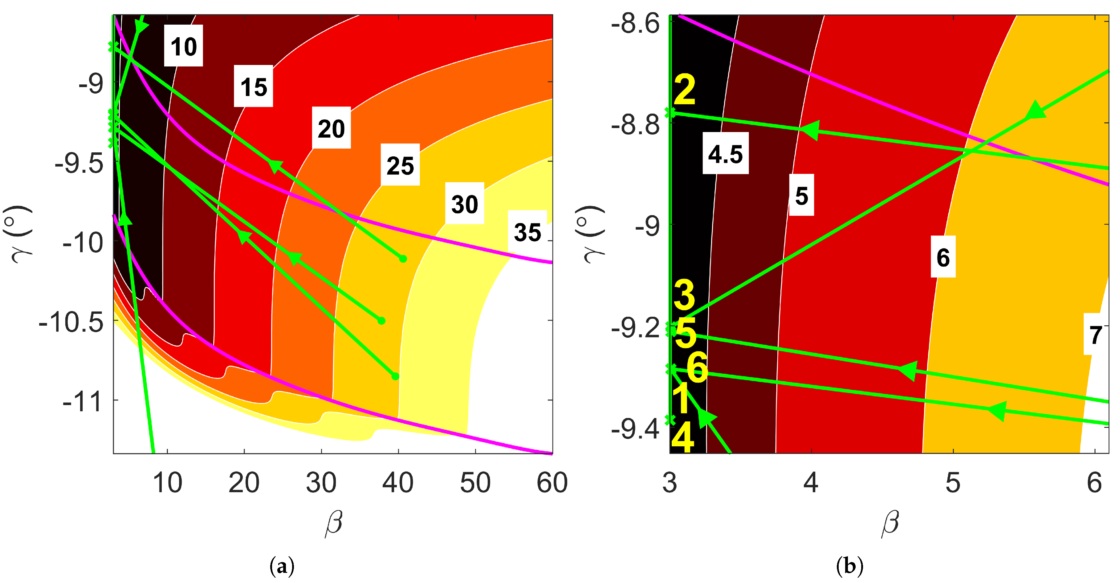
Figure A3.
Aerocapture trajectory profiles resulting from minimal heat load mission design,
, with default fmincon convergence criteria (a) Altitude vs velocity. (b) Altitude and vs time.
Figure A3.
Aerocapture trajectory profiles resulting from minimal heat load mission design,
, with default fmincon convergence criteria (a) Altitude vs velocity. (b) Altitude and vs time.
Appendix D. Minimum Heat Load Trajectory: Local minima vs Global minima at β=3
Figure A4.
Local vs. global minima in minimum heat load trajectory, blue cross, and green dot respectively.
Figure A4.
Local vs. global minima in minimum heat load trajectory, blue cross, and green dot respectively.
Appendix E. Impact of Binary Search Tolerance on Polynomial Fits
Figure A5.
Accuracy evolution of sixth-degree polynomial curves as a function of binary search tolerance used for computing fitting points. (a) Corridor boundaries. (b) Lower bound fit. (c) Upper bound fit.
Figure A5.
Accuracy evolution of sixth-degree polynomial curves as a function of binary search tolerance used for computing fitting points. (a) Corridor boundaries. (b) Lower bound fit. (c) Upper bound fit.
References
- Jorris, T.R.; Cobb, R.G. Three-Dimensional Trajectory Optimization Satisfying Waypoint and No-Fly Zone Constraints. Journal of Guidance, Control, and Dynamics 2009, 32, 551–572. [Google Scholar] [CrossRef]
- Liu, X.; Shen, Z.; Lu, P. Entry Trajectory Optimization by Second-Order Cone Programming. Journal of Guidance, Control, and Dynamics 2016, 39, 227–241. [Google Scholar] [CrossRef]
- Li, Y.; Sun, G.; Han, H. Aerocapture Optimization Method with Lift–Drag Joint Modulation Suitable for Variable Structure Spacecraft. Aerospace 2023, 10, 24. [Google Scholar] [CrossRef]
- Lu, P.; Cerimele, C.; Tigges, M.; Matz, D. Optimal Aerocapture Guidance. Journal of Guidance, Control, and Dynamics 2015, 38, 553–565. [Google Scholar] [CrossRef]
- Heidrich, C.; Roelke, E.; Albert, S.; Braun, R. Comparative Study Of Lift-And Drag-Modulation Control Strategies For Aerocapture. 01 2020.
- Han, H.; Qiao, D.; Chen, H.; Li, X. Rapid planning for aerocapture trajectory via convex optimization. Aerospace Science and Technology 2019, 84, 763–775. [Google Scholar] [CrossRef]
- Girija, A.P.; Saikia, S.J.; Longuski, J.M.; Cutts, J.A. AMAT: A Python package for rapid conceptual design of aerocapture and atmospheric Entry, Descent, and Landing (EDL) missions in a Jupyter environment. Journal of Open Source Software 2021, 6, 3710. [Google Scholar] [CrossRef]
- Girija, A.P. A Systems Framework and Analysis Tool for Rapid Conceptual Design of Aerocapture Missions. PhD thesis, Purdue University, 2021. Copyright - Database copyright ProQuest LLC; ProQuest does not claim copyright in the individual underlying works; Last updated - 2024-07-18.
- Kumar, M.; Tewari, A. Trajectory and Attitude Simulation for Aerocapture and Aerobraking. Journal of Spacecraft and Rockets 2005, 42. [Google Scholar] [CrossRef]
- Sutton, K.; Graves, R.A. A general stagnation-point convective heating equation for arbitrary gas mixtures; NASA TR R-376, 1971.
- Tauber, M.E.; Sutton, K. Stagnation-point radiative heating relations for Earth and Mars entries. Journal of Spacecraft and Rockets 1991, 28, 40–42. [Google Scholar] [CrossRef]
- U.S. Standard Atmosphere; U.S. Government Printing Office: Washington, D.C, 1962.
- Hall, N. Earth Atmopshere Model - Metric Units; NASA - Glenn Research Center, 2021.
- Leslie, F.W.; Justus, C.G. The NASA Marshall Space Flight Center Earth Global Reference Atmospheric Model—2010 Version; NASA-TM-2011-216467, 2001.
- Jursa, A.S. Handbook of Geophysics and the Space Envvironment; Air Force Geophysics Laboratory, 1985.
- Justus, C.; Duvall, A.; Keller, V. , Atmospheric Models for Mars Aerocapture; 41st AIAA/ASME/SAE/ASEE Joint Propulsion Conference & Exhibit, American Institute of Aeronautics and Astronautics, 2005. [CrossRef]
- Curtis, H.D. Orbital mechanics for engineering students; Elsevier Butterworth Heinemann Amsterdam: Amsterdam, 2005. [Google Scholar]
- Edquist, K. Computations of Viking Lander Capsule Hypersonic Aerodynamics with Comparisons to Ground and Flight Data. AIAA Atmospheric Flight Mechanics Conference and Exhibit 2006. [Google Scholar] [CrossRef]
- Gill, P.E.; Murray, W.; Wright, M.H. Practical Optimization; Acamademic Press, 1997.
- Allen, H.J.; Eggers, A.J. A Study of the Motion and Aerodynamic Heating of Ballistic Missiles Entering the Earth’s Atmosphere at HighSupersonic Speeds; NACA TR-1381, 1958.
Figure 2.
Martian and Terrestrial aerocapture corridors for multiple hyperbolic excess velocities, . The polynomial fits for low, mean, and high-density corridor boundaries are shown: (a) Martian aerocapture corridor with . (b) Martian aerocapture corridor with . (c) Terrestrial aerocapture corridor with
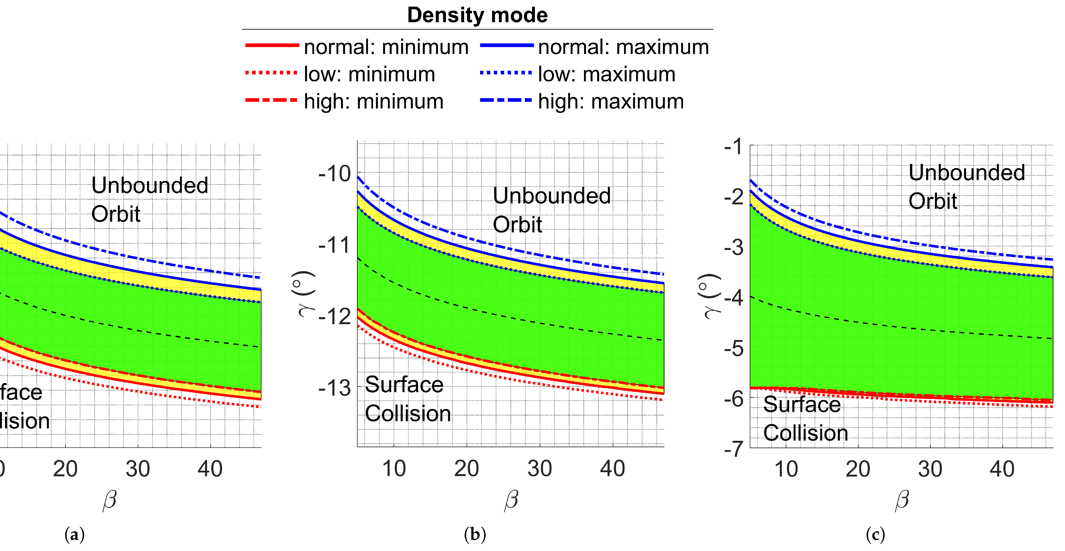
Figure 3.
Percentage error between finely discretized corridor limits (570 points) and computed values using exponential and polynomial constructed from 7 points. (a) Earth, . (b) Earth, . (c) Earth, . (d) Mars, . (e) Mars, . (f) Mars, .
Figure 3.
Percentage error between finely discretized corridor limits (570 points) and computed values using exponential and polynomial constructed from 7 points. (a) Earth, . (b) Earth, . (c) Earth, . (d) Mars, . (e) Mars, . (f) Mars, .
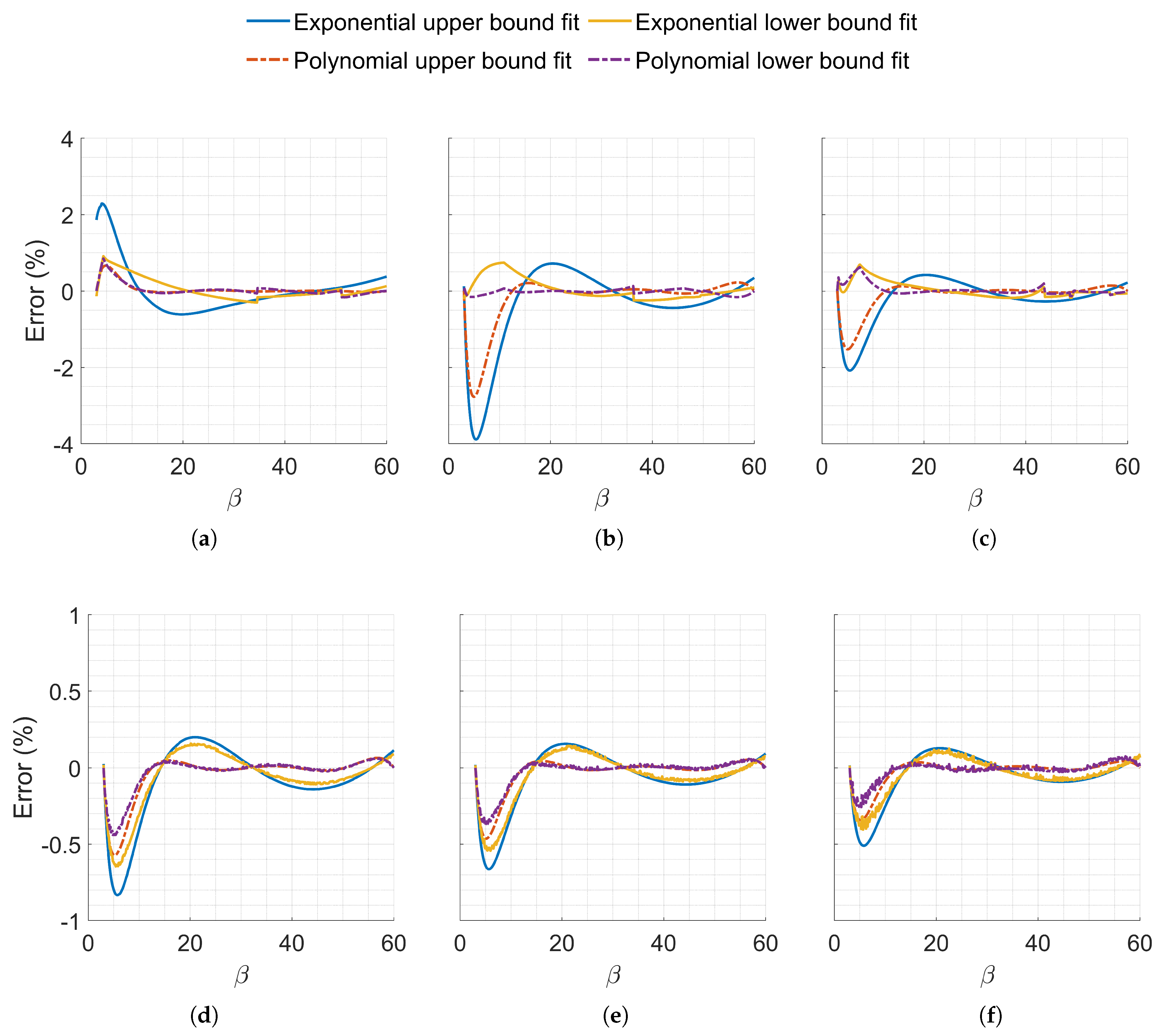
Figure 4.
Coarse robust Martian aerocapture corridor for used to compute normalization quantities listed in Table 1 and sixth-degree polynomial fits.
Figure 4.
Coarse robust Martian aerocapture corridor for used to compute normalization quantities listed in Table 1 and sixth-degree polynomial fits.
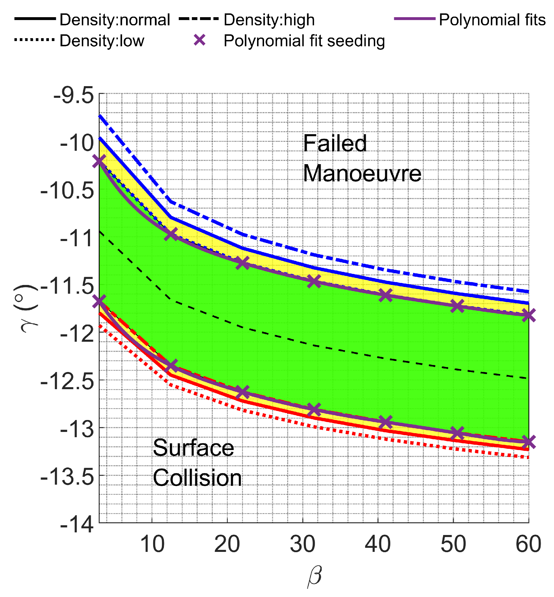
Figure 5.
Convergence property of D-ASTRO for overall optimal mission design, , with magenta lines delineating the boundaries of the aerocapture corridor. (a) Convergence of to . (b) Zoom into global minimum region
Figure 5.
Convergence property of D-ASTRO for overall optimal mission design, , with magenta lines delineating the boundaries of the aerocapture corridor. (a) Convergence of to . (b) Zoom into global minimum region
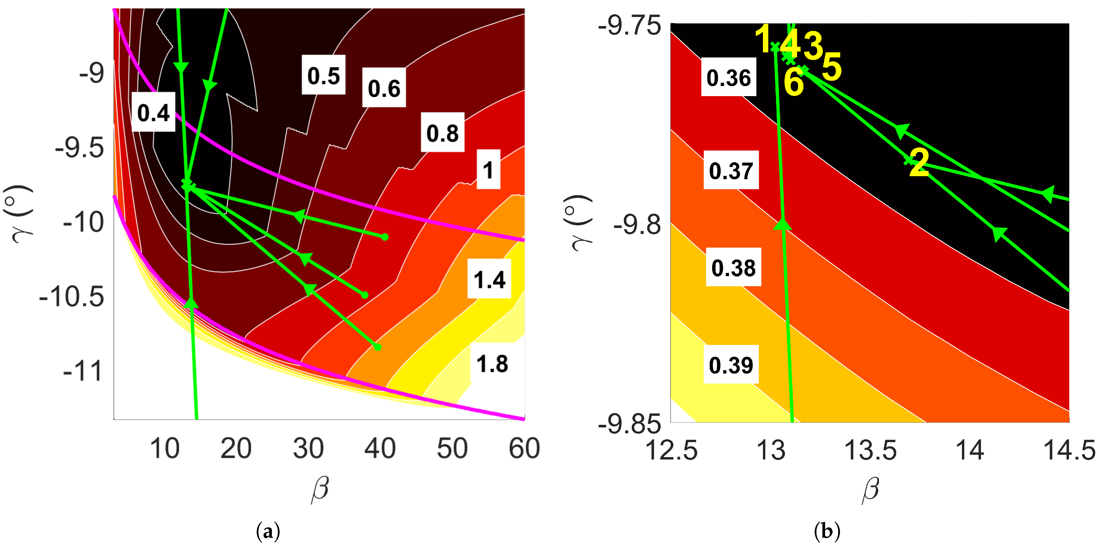
Figure 6.
Aerocapture trajectory profiles resulting from overall optimal mission design, .
(a) Altitude vs velocity. (b) Altitude and vs time.
Figure 6.
Aerocapture trajectory profiles resulting from overall optimal mission design, .
(a) Altitude vs velocity. (b) Altitude and vs time.
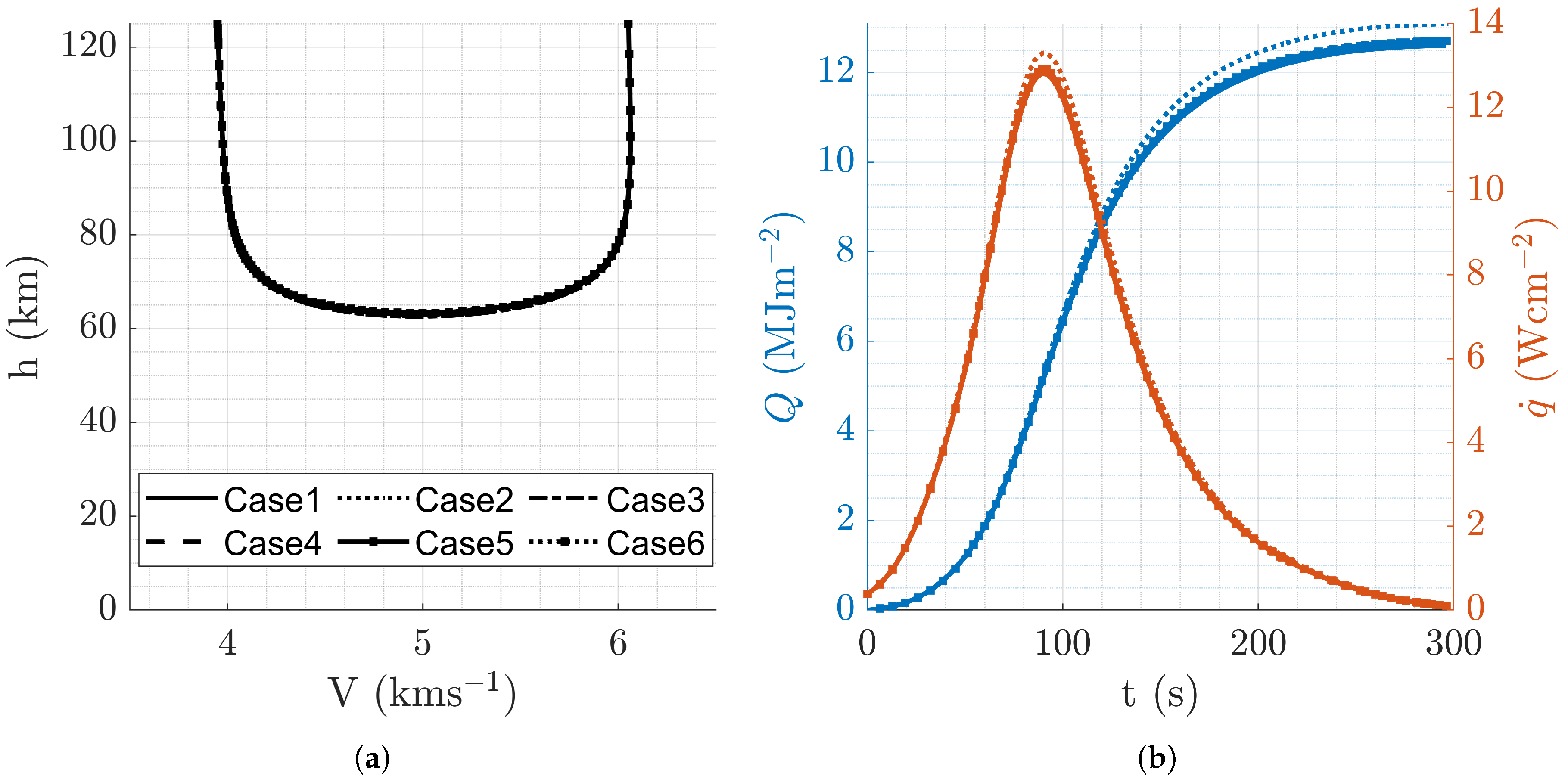
Figure 7.
Convergence property of D-ASTRO for minimum fuel mission design, , with magenta lines delineating the boundaries of the aerocapture corridor. (a) Convergence of to . (b) Zoom into global minimum region.
Figure 7.
Convergence property of D-ASTRO for minimum fuel mission design, , with magenta lines delineating the boundaries of the aerocapture corridor. (a) Convergence of to . (b) Zoom into global minimum region.
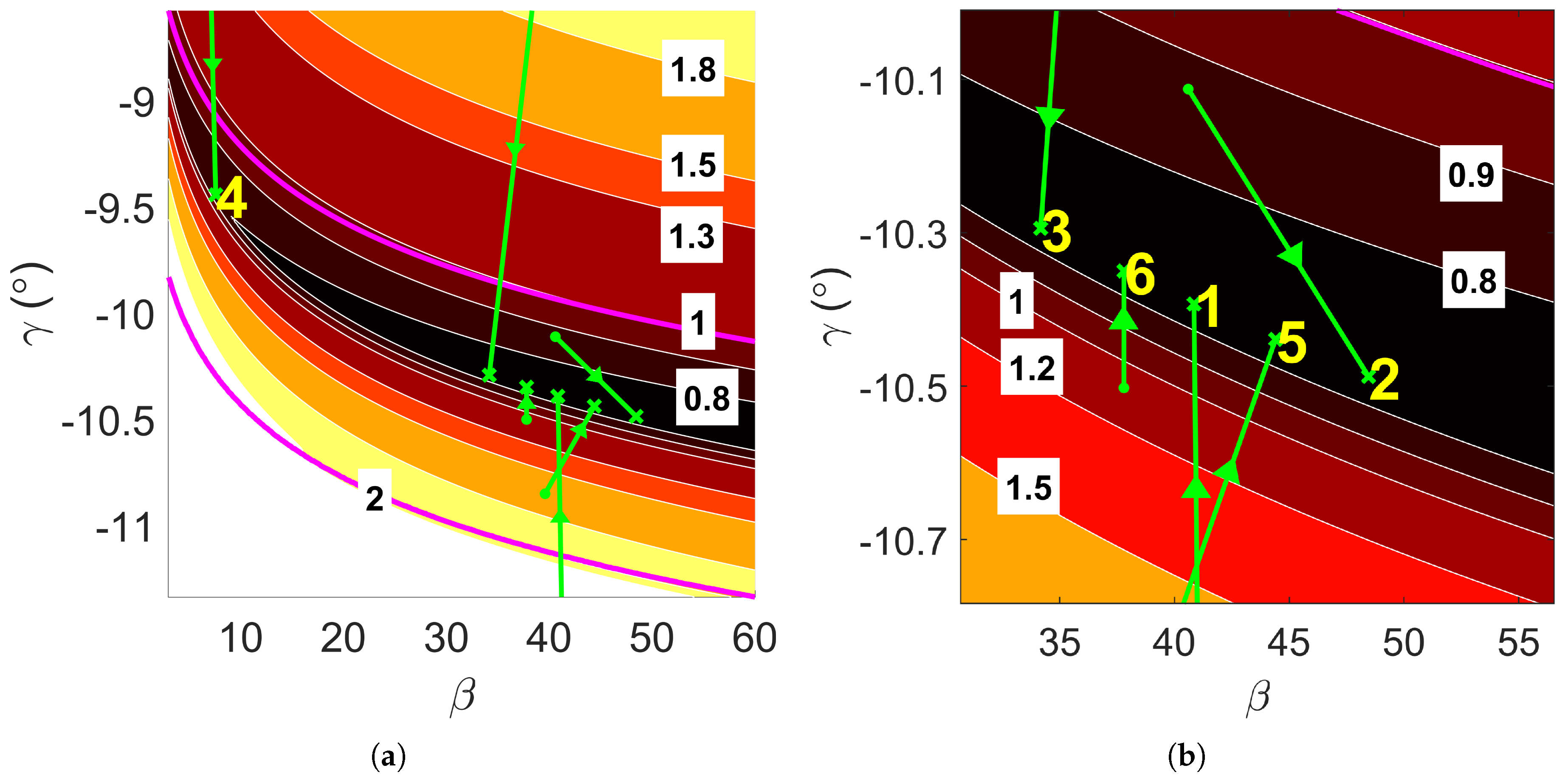
Figure 8.
contours for minimal fuel trajectory neglecting plane change maneuvers, , and .
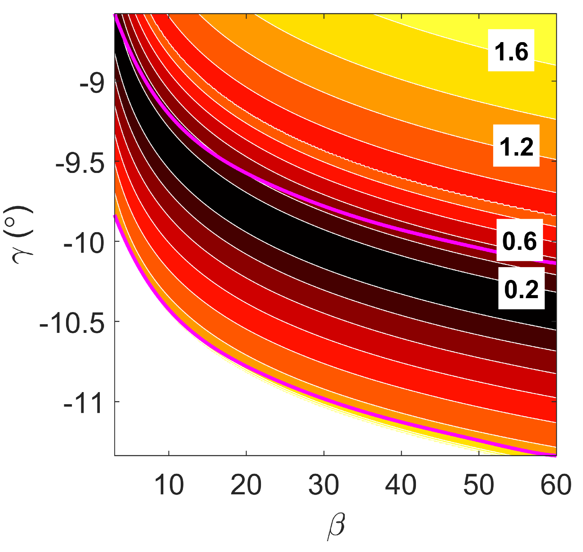
Figure 9.
Aerocapture trajectory profiles resulting from minimal fuel mission design, .
(a) Altitude vs velocity. (b) Altitude and vs time.
Figure 9.
Aerocapture trajectory profiles resulting from minimal fuel mission design, .
(a) Altitude vs velocity. (b) Altitude and vs time.
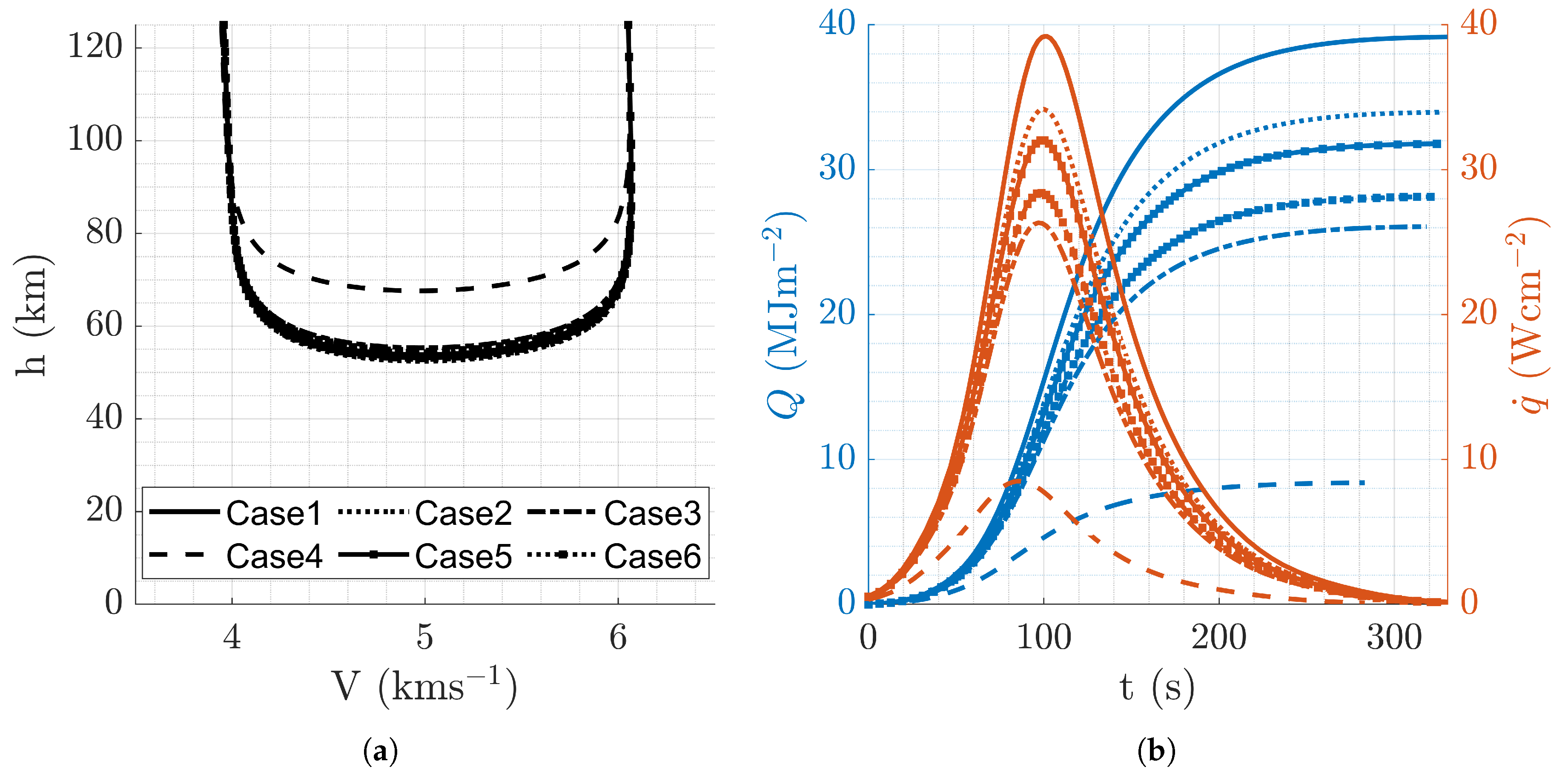
Figure 10.
Convergence property of D-ASTRO for minimum heat load mission design, , with magenta lines delineating the boundaries of the aerocapture corridor. (a) Convergence of to . (b) Zoom into global minimum region.
Figure 10.
Convergence property of D-ASTRO for minimum heat load mission design, , with magenta lines delineating the boundaries of the aerocapture corridor. (a) Convergence of to . (b) Zoom into global minimum region.
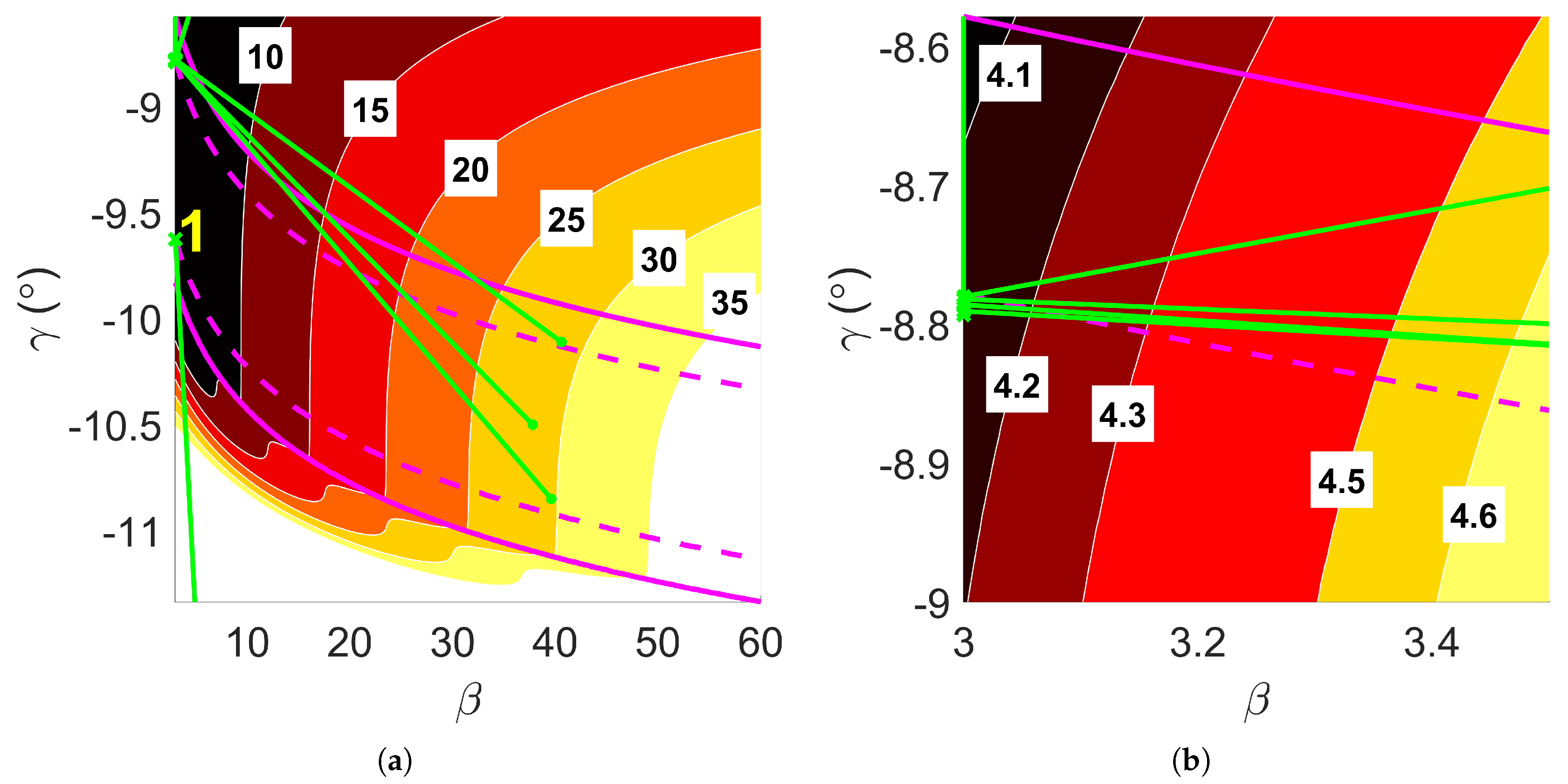
Figure 11.
Normalized heat load, . (a) Complete trajectory analysis. (b) Predicted by Equation 16.
Figure 11.
Normalized heat load, . (a) Complete trajectory analysis. (b) Predicted by Equation 16.
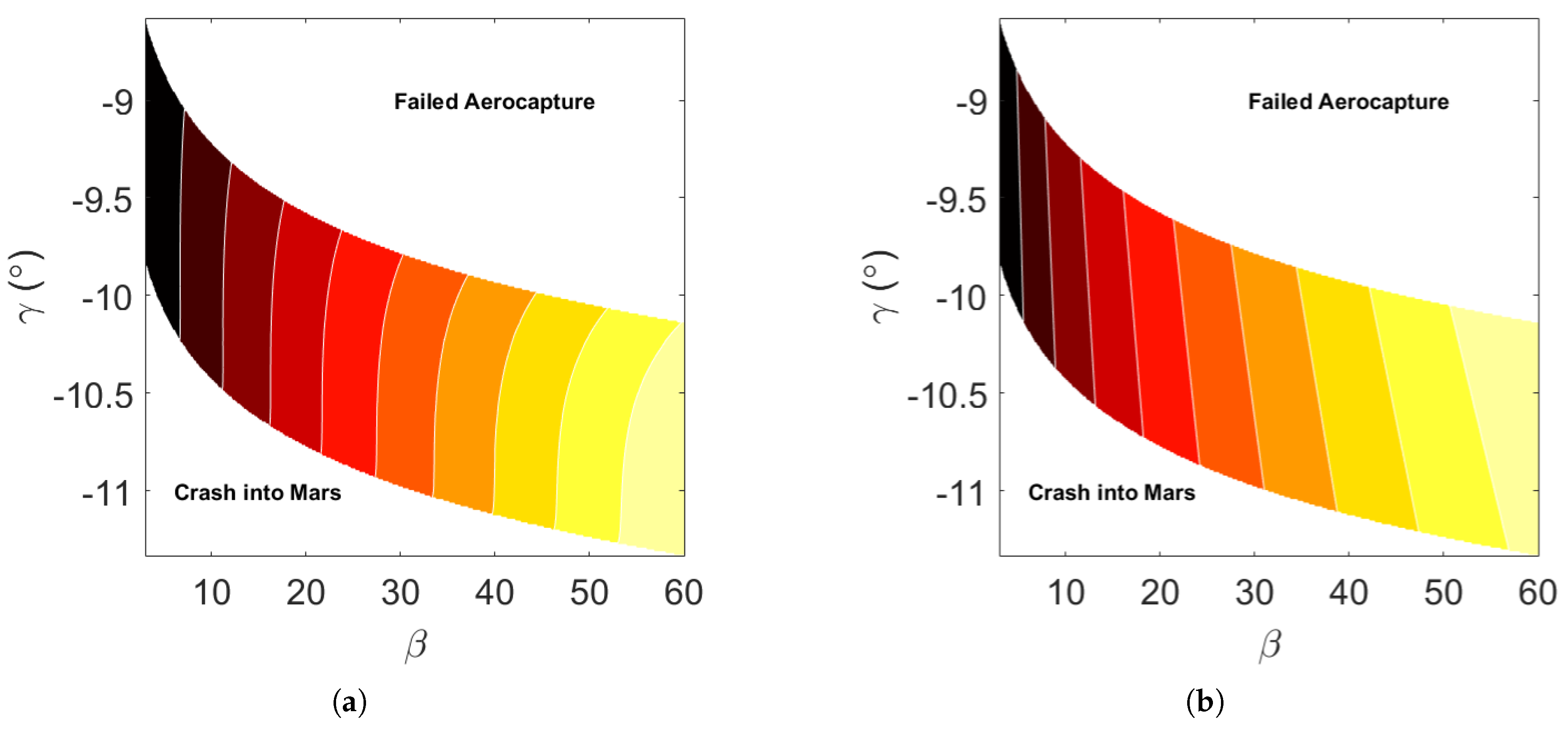
Figure 12.
Aerocapture trajectory profiles resulting from minimal heat load mission design,
. (a) Altitude vs velocity. (b) Altitude and vs time.
Figure 12.
Aerocapture trajectory profiles resulting from minimal heat load mission design,
. (a) Altitude vs velocity. (b) Altitude and vs time.
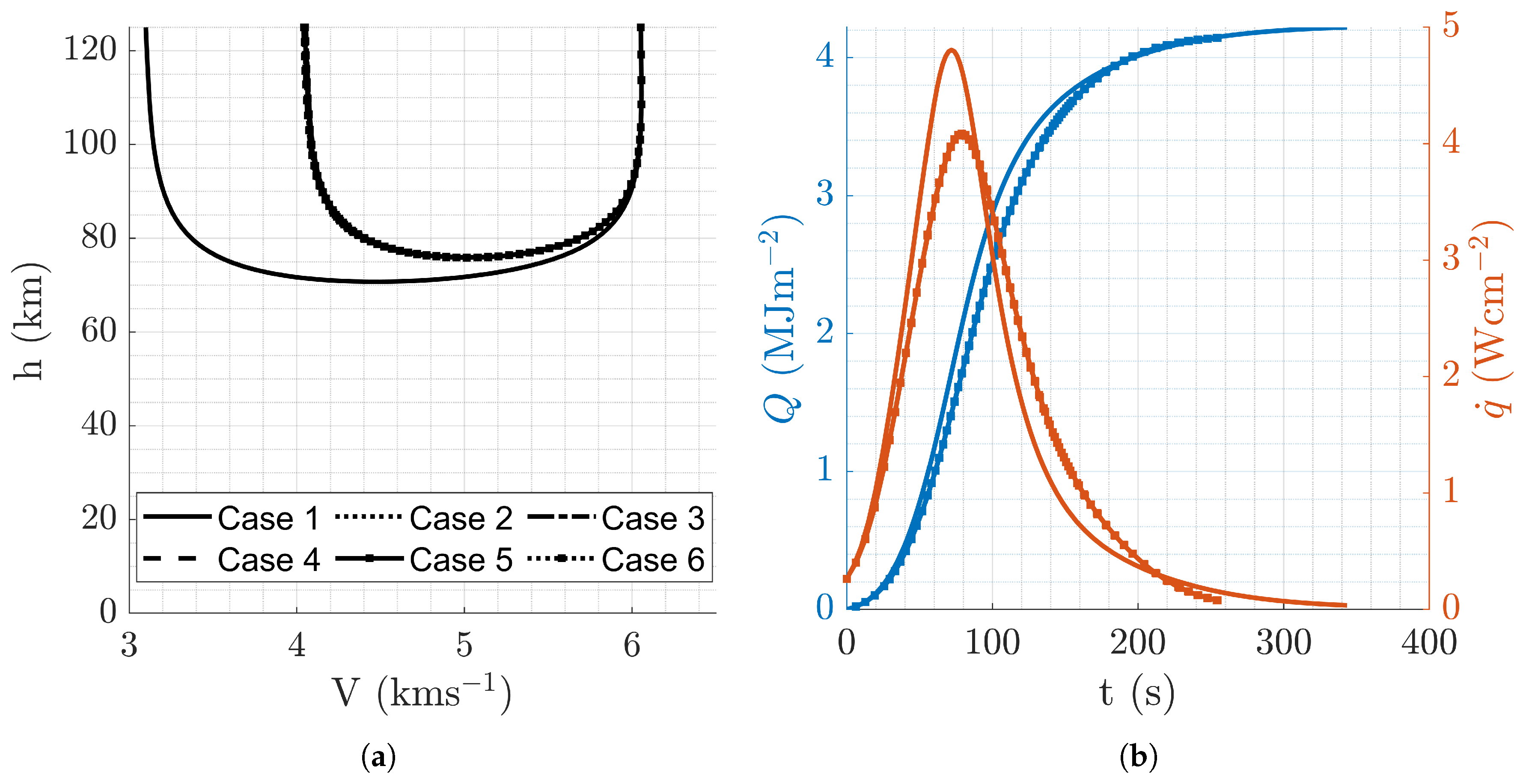
Figure 13.
Convergence property of D-ASTRO for minimum peak heating rate mission design, , with magenta lines delineating the boundaries of the aerocapture corridor. (a) Convergence of to . (b) Zoom into global minimum region.
Figure 13.
Convergence property of D-ASTRO for minimum peak heating rate mission design, , with magenta lines delineating the boundaries of the aerocapture corridor. (a) Convergence of to . (b) Zoom into global minimum region.
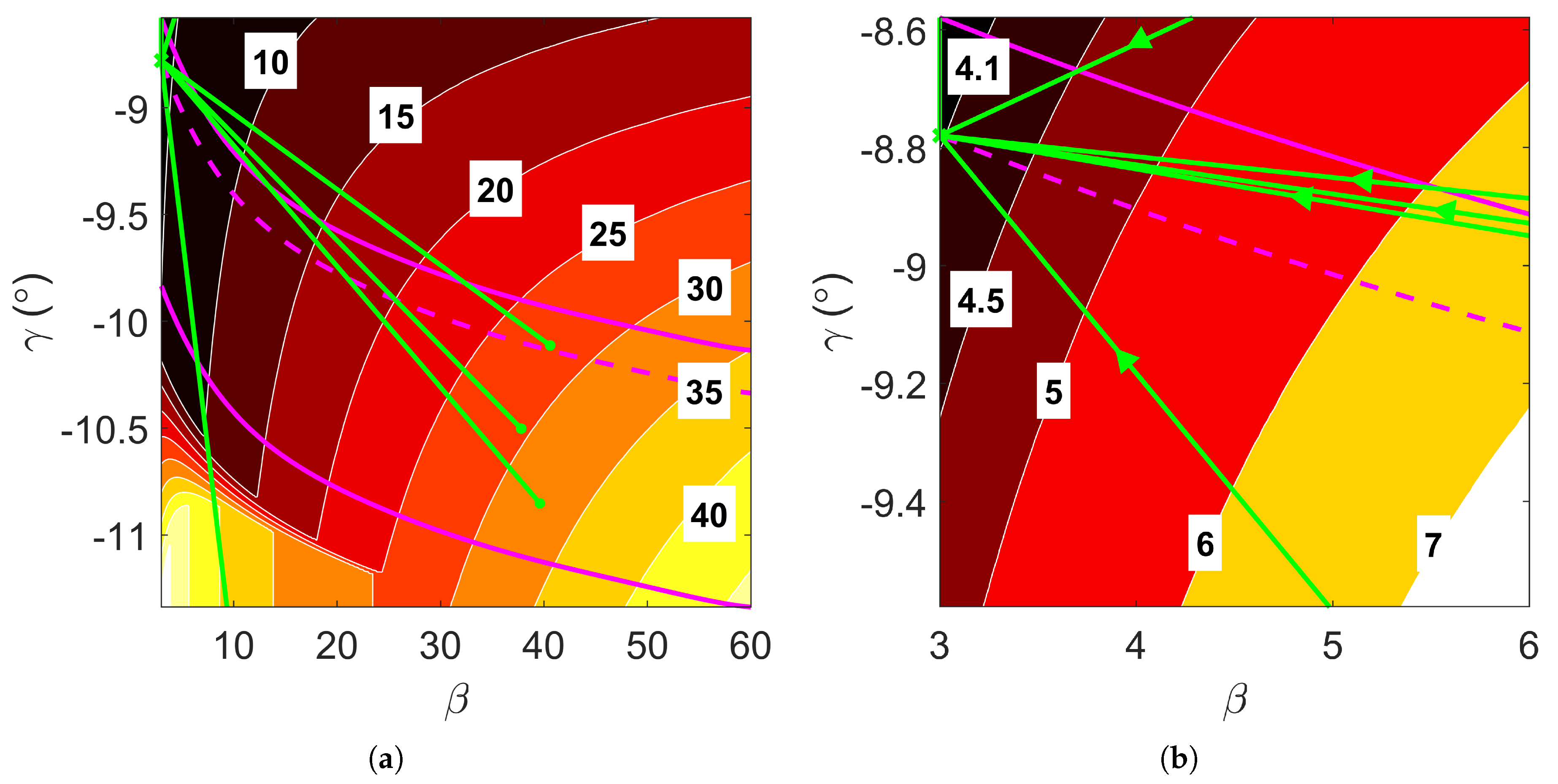
Figure 14.
Aerocapture trajectory profiles resulting from minimal peak heating rate mission design, . (a) Altitude vs velocity. (b) Altitude and vs time.
Figure 14.
Aerocapture trajectory profiles resulting from minimal peak heating rate mission design, . (a) Altitude vs velocity. (b) Altitude and vs time.
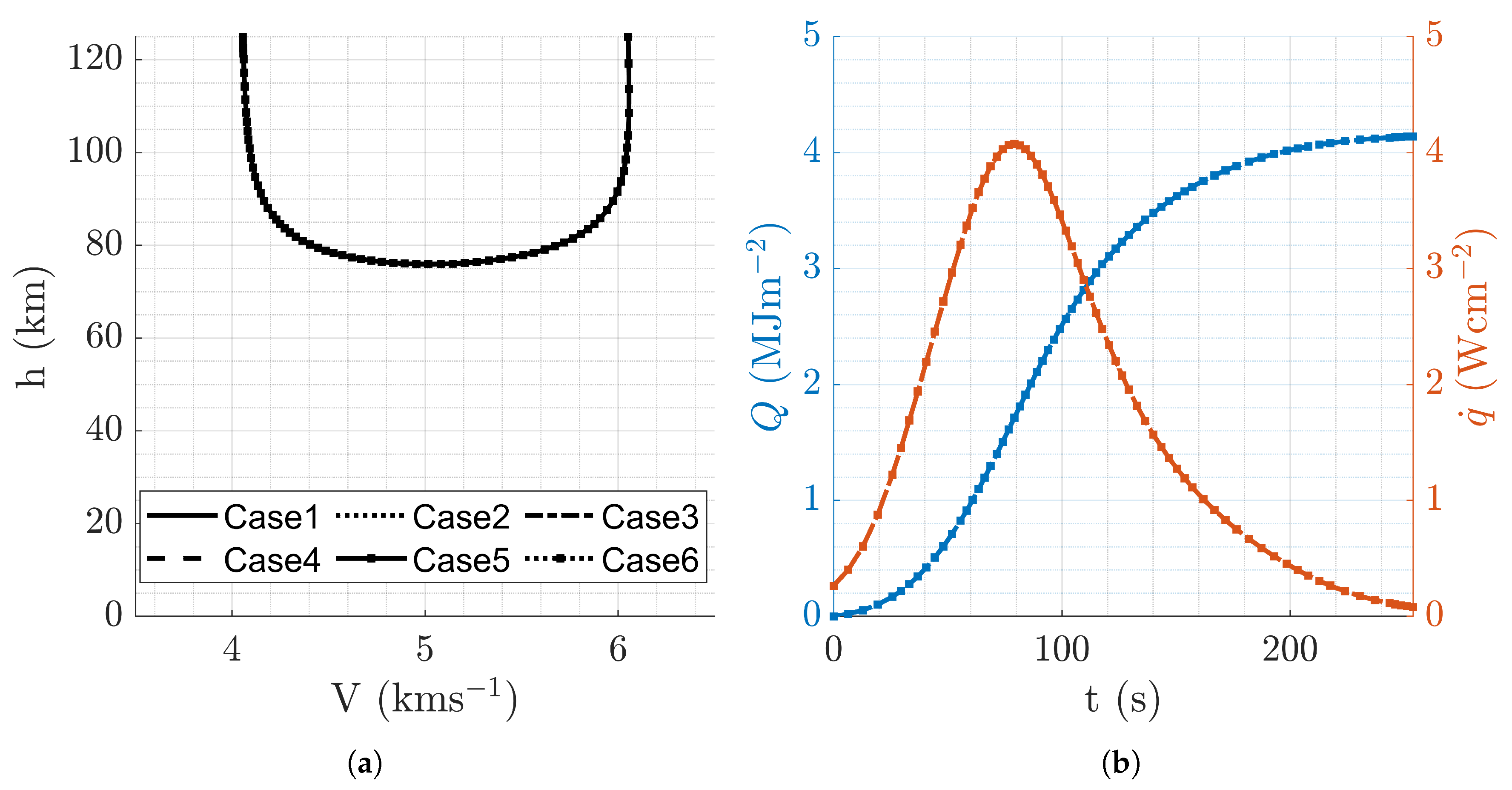
Figure 15.
Convergence property of MOO strategy for overall optimal mission design (blue) compared with D-ASTRO (green), , with magenta lines delineating the aerocapture boundaries.
Figure 15.
Convergence property of MOO strategy for overall optimal mission design (blue) compared with D-ASTRO (green), , with magenta lines delineating the aerocapture boundaries.
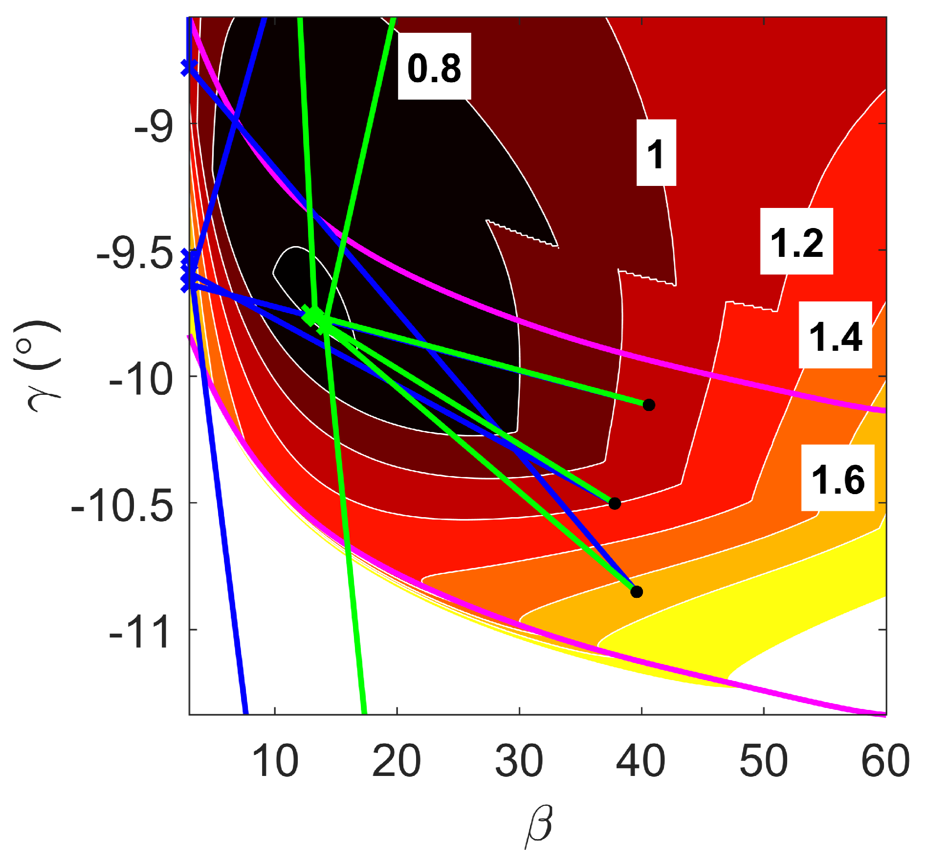
Figure 16.
Aerocapture trajectory profiles resulting from overall optimal mission design using MOO strategy, . (a) Altitude vs velocity. (b) Altitude and vs time.
Figure 16.
Aerocapture trajectory profiles resulting from overall optimal mission design using MOO strategy, . (a) Altitude vs velocity. (b) Altitude and vs time.
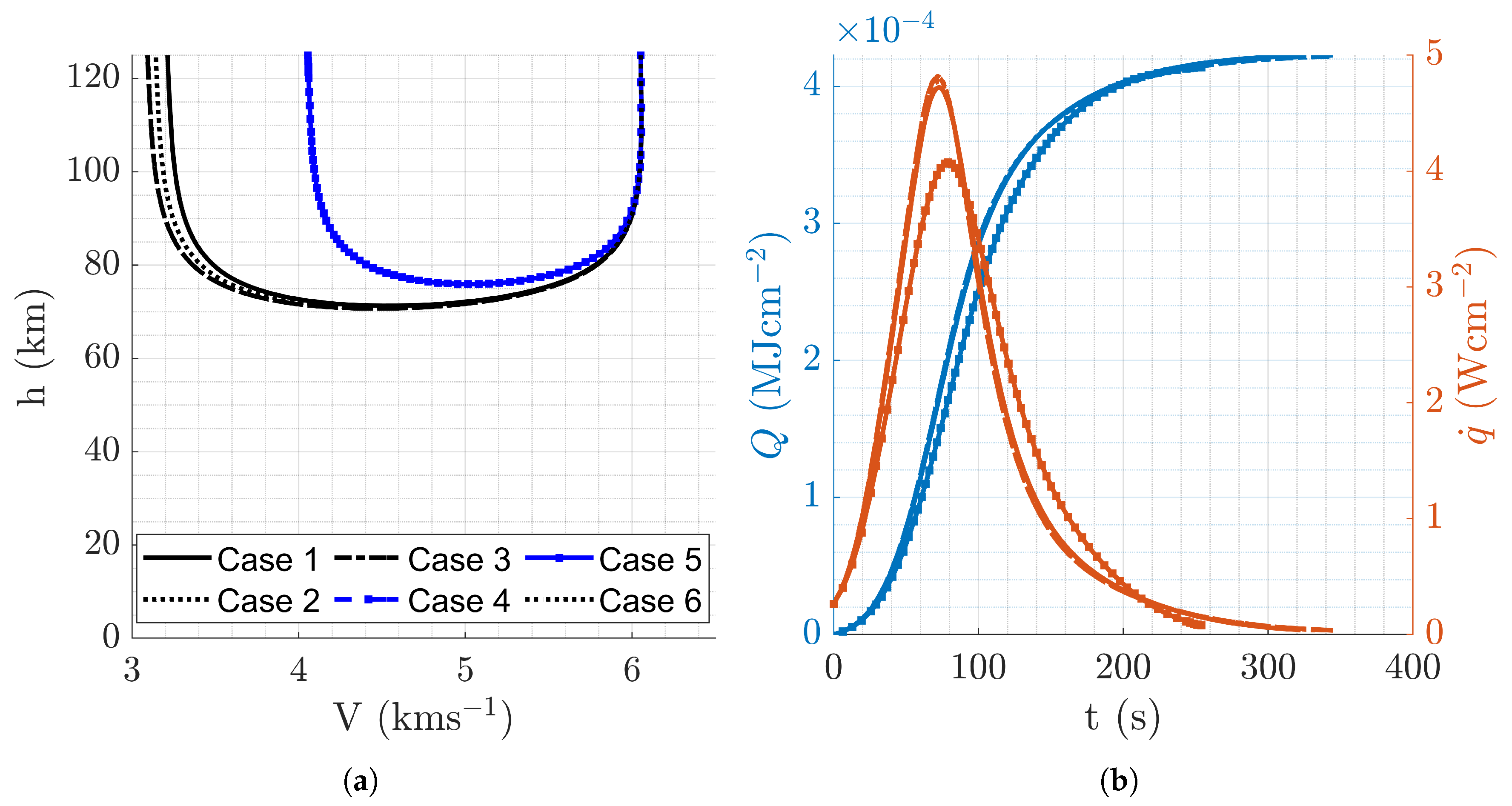
Figure 17.
Aerocapture trajectory profiles resulting from all optimal mission designs presented in this study. Initial conditions correspond to those that result in the lowest cost. (a) Altitude vs velocity. (b) Altitude and vs time.
Figure 17.
Aerocapture trajectory profiles resulting from all optimal mission designs presented in this study. Initial conditions correspond to those that result in the lowest cost. (a) Altitude vs velocity. (b) Altitude and vs time.
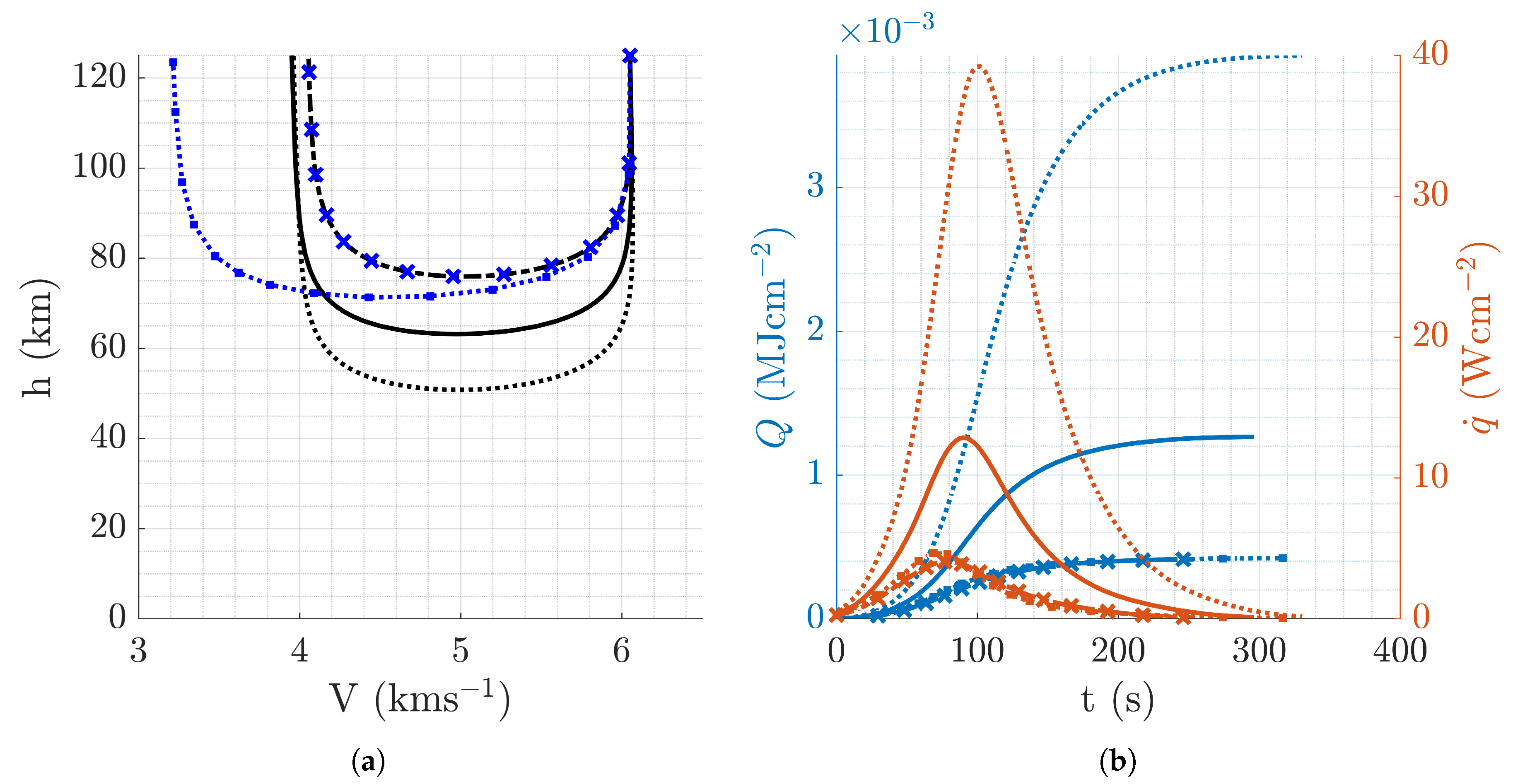
Figure 18.
Evolution of Euclidean L-2 norm of upper and lower boundary fits and execution time of robust coarse aerocapture corridor. (a) Martian Aerocapture, . (b) Terrestrial Aerocapture,
Figure 18.
Evolution of Euclidean L-2 norm of upper and lower boundary fits and execution time of robust coarse aerocapture corridor. (a) Martian Aerocapture, . (b) Terrestrial Aerocapture,
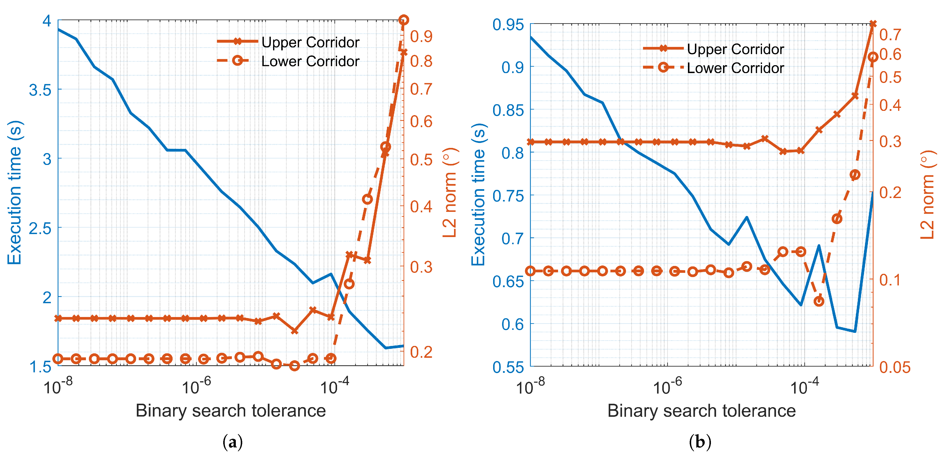
Table 1.
Minimum and maximum values of considered metrics for a Martian aerocapture corridor for
.
| Variable | Minimum | Maximum |
|---|---|---|
| 1.15 | 5.15 | |
| 0.00 | 3.56 | |
| Q | 3.42 | 41.53 |
| 3.45 | 46.32 |
Table 2.
Martian aerocapture simulation parameters
| Parameter | Value | Parameter | Value | ||
|---|---|---|---|---|---|
| Planetary parameters | Insertion trajectory parameters | ||||
| Radius of Mars, | 3,390 | km | Hyperbolic excess velocity, | 3.5 | |
| Gravitational parameter, | Atmospheric interface altitude, | 125 | |||
| Angular frequency of Mars, | Initial Radius, | ||||
| Vehicle parameters | Initial velocity, | ||||
| Mass of vehicles, m | 400 | Initial longitude, | 0.5798 | ||
| Drag coefficient, | 1.6 | Initial latitude, | 34.49 | ||
| Lift-to-Drag ration, | 0.2 | Initial heading angle, | -18.24 | ||
| Nose radius to Body radius ratio, | 0.5 | Insertion flight path angle accuracy, | |||
Table 3.
Target Operational orbit
| Target parameter | Semi-major axis, a | Inclination, i | Eccentricity, e |
|---|---|---|---|
| Value | 4,621 | 70 | 0.05 |
Table 4.
Convergence properties of optimization algorithm with different initial conditions
| Case | Initial Conditions | Cost | Optimized Parameters | Performance Metrics | |||||
|---|---|---|---|---|---|---|---|---|---|
| () | () | () | () | Q () | () | ||||
| 1 | 59.0 | -60.000 | 0.5280 | 13.03 | -9.756 | 2.472 | 0.777 | 12.608 | 12.805 |
| 2 | 40.6 | -10.113 | 0.5280 | 13.69 | -9.784 | 2.411 | 0.776 | 13.094 | 13.301 |
| 3 | 59.0 | -0.057 | 0.5303 | 13.08 | -9.758 | 2.467 | 0.778 | 12.649 | 12.846 |
| 4 | 3.0 | -0.057 | 0.5283 | 13.10 | -9.759 | 2.465 | 0.778 | 12.665 | 12.862 |
| 5 | 39.6 | -10.852 | 0.5280 | 13.17 | -9.762 | 2.458 | 0.778 | 12.714 | 12.913 |
| 6 | 37.8 | -10.502 | 0.5283 | 13.16 | -9.762 | 2.459 | 0.778 | 12.704 | 12.902 |
Table 5.
Optimal results for minimum fuel trajectory
| Case | () | Cost | () | () | ||
|---|---|---|---|---|---|---|
| 1 | 59.0 | -60.000 | 0.1092 | 40.85 | -10.393 | 0.7163 |
| 2 | 40.6 | -10.113 | 0.1064 | 48.46 | -10.487 | 0.7070 |
| 3 | 59.0 | -0.057 | 0.1122 | 34.17 | -10.294 | 0.7259 |
| 4 | 3.0 | -0.057 | 0.1392 | 7.58 | -9.445 | 0.8087 |
| 5 | 39.6 | -10.852 | 0.1078 | 44.40 | -10.439 | 0.7117 |
| 6 | 37.8 | -10.502 | 0.1105 | 37.80 | -10.350 | 0.7205 |
Table 6.
Optimal results for minimum heat load trajectory
| Case | () | Cost | () | Q () | ||
|---|---|---|---|---|---|---|
| 1 | 59.0 | -60.000 | 3.00 | -9.6289 | 4.221 | |
| 2 | 40.6 | -10.113 | 3.00 | -8.7822 | 4.141 | |
| 3 | 59.0 | -0.057 | 3.00 | -8.7803 | 4.140 | |
| 4 | 3.0 | -0.057 | 3.00 | -8.7934 | 4.145 | |
| 5 | 39.6 | -10.852 | 3.00 | -8.7862 | 4.142 | |
| 6 | 37.8 | -10.502 | 3.00 | -8.7908 | 4.144 |
Table 7.
Optimal results for minimal trajectory.
| Case | () | Cost | () | () | (deg) | ||
|---|---|---|---|---|---|---|---|
| 1 | 59.0 | -60.000 | 7.92 | 3.0 | -8.780 | 4.0754 | 0.2000 |
| 2 | 40.6 | -10.113 | 7.92 | 3.0 | -8.780 | 4.0754 | 0.2000 |
| 3 | 59.0 | -0.057 | 7.92 | 3.0 | -8.780 | 4.0754 | 0.2000 |
| 4 | 3.0 | -0.057 | 7.92 | 3.0 | -8.780 | 4.0754 | 0.2000 |
| 5 | 39.6 | -10.852 | 7.92 | 3.0 | -8.780 | 4.0754 | 0.2000 |
| 6 | 37.8 | -10.502 | 7.92 | 3.0 | -8.780 | 4.0754 | 0.2000 |
Table 8.
Convergence properties of MOO algorithm and D-ASTRO for overall optimal trajectory.
| Case | () | Strategy | () | () | () | Q () | () | ||
|---|---|---|---|---|---|---|---|---|---|
| 1 | 59.0 | -60.000 | MOO | 3.000 | -9.526 | 5.150 | 1.969 | 4.225 | 4.723 |
| D-ASTRO | 13.03 | -9.756 | 2.472 | 0.779 | 12.608 | 12.805 | |||
| 2 | 40.6 | -10.113 | MOO | 3.007 | -9.635 | 5.145 | 2.062 | 4.228 | 4.818 |
| D-ASTRO | 13.69 | -9.784 | 2.411 | 0.776 | 13.094 | 13.301 | |||
| 3 | 59.0 | -0.057 | MOO | 3.000 | -9.635 | 5.150 | 2.063 | 4.221 | 4.810 |
| D-ASTRO | 13.08 | -9.758 | 2.467 | 0.778 | 12.649 | 12.846 | |||
| 4 | 3.0 | -0.057 | MOO | 3.000 | -8.780 | 5.150 | 0.884 | 4.140 | 4.075 |
| D-ASTRO | 13.10 | -9.759 | 2.465 | 0.778 | 12.665 | 12.862 | |||
| 5 | 39.6 | -10.852 | MOO | 3.000 | -8.780 | 5.150 | 0.884 | 4.140 | 4.075 |
| D-ASTRO | 13.17 | -9.762 | 2.458 | 0.778 | 12.714 | 12.913 | |||
| 6 | 37.8 | -10.502 | MOO | 3.000 | -9.590 | 5.150 | 2.025 | 4.222 | 4.774 |
| D-ASTRO | 13.16 | -9.762 | 2.459 | 0.778 | 12.704 | 12.902 |
Table 10.
Computational Performance and Suggested Optima of D-ASTRO and MOO strategies without employing polynomial fits to evaluate and . and used as initial guess for Martian test case.
Table 10.
Computational Performance and Suggested Optima of D-ASTRO and MOO strategies without employing polynomial fits to evaluate and . and used as initial guess for Martian test case.
| weights | Strategy | Execution time (s) | Function counts | Time per function call (ms) | ||
|---|---|---|---|---|---|---|
| D-ASTRO | 65.1 | 202 | 322 | 12.22 | -9.719 | |
| MOO | 90.2 | 304 | 297 | 3.00 | -9.634 | |
| D-ASTRO | 48.9 | 162 | 302 | 40.60 | -10.390 | |
| MOO | 93.1 | 304 | 306 | 21.78 | -8.501 | |
| D-ASTRO | 71.0 | 202 | 3528 | 16.00 | -9.657 | |
| MOO | 109 | 301 | 363 | 12.39 | -9.853 |
Table 11.
Percentage difference in performance metrics when fits and binary search are used to assess the feasibility of candidate points.
Table 11.
Percentage difference in performance metrics when fits and binary search are used to assess the feasibility of candidate points.
| weights | Strategy | Percentage Difference (%) | |||
|---|---|---|---|---|---|
| Q | |||||
| D-ASTRO | 4.036 | 0.566 | -5.781 | -5.798 | |
| MOO | 0.454 | 0.097 | -0.682 | -0.673 | |
| D-ASTRO | 4.066 | 0.604 | -5.842 | -5.804 | |
| MOO | 36.545 | 92.352 | -58.701 | -62.593 | |
| D-ASTRO | -1.327 | 0.526 | 1.895 | 1.672 | |
| MOO | 0.000 | -0.046 | -0.001 | -0.005 | |
Disclaimer/Publisher’s Note: The statements, opinions and data contained in all publications are solely those of the individual author(s) and contributor(s) and not of MDPI and/or the editor(s). MDPI and/or the editor(s) disclaim responsibility for any injury to people or property resulting from any ideas, methods, instructions or products referred to in the content. |
© 2025 by the authors. Licensee MDPI, Basel, Switzerland. This article is an open access article distributed under the terms and conditions of the Creative Commons Attribution (CC BY) license (http://creativecommons.org/licenses/by/4.0/).
Copyright: This open access article is published under a Creative Commons CC BY 4.0 license, which permit the free download, distribution, and reuse, provided that the author and preprint are cited in any reuse.


