Submitted:
10 June 2023
Posted:
12 June 2023
You are already at the latest version
Abstract
The complexity of objects and control systems increases the requirements for mathematical models. The structural identifiability (SI) assessment of nonlinear systems is one of the identification problems. Until now, this problem solves by parametric methods using various approximation methods. This approach is not always effective under uncertainty. We apply an approach to SI estimation based on the analysis of virtual structures. The requirements form for the system input based on the expansion of the excitation constancy property and S-synchronizability. The approach generalization to structural identifiability used in the analysis of systems with symmetric nonlinearity is given. homothety and identifiability conditions for systems with non-symmetric nonlinearities (SNN) obtained. The detectability and recoverability proofed for virtual frameworks (VF) guaranteed the SI estimation under uncertainty. The conditions under which the non-symmetric nonlinearity is hypothetical symmetric nonlinearity obtained. SI estimation examples considered for closed nonlinear systems under uncertainty.
Keywords:
nonsymmetric nonlinearity
; nonlinear dynamical system
; virtual structure
; S-synchronizability
; excitation constancy
; homotety
; feedback
; structural identifiability
1. Introduction
Nonsymmetric nonlinear systems used to control various objects [1,2,3,4,5]. A genetic procedure [1] proposed for the nonsymmetric hysteresis identification. In [2], an extended Prandtl-Ishlinskii model based on the application of the asymmetric reproduction operator proposed. Its analogue is used in [1]. In [3,4], models propose considering the influence of the excitation frequency on the hysteresis. A generalized Bouc-Wen model [5] proposed to describe strongly asymmetric hysteresis. Inverse motion control scheme [6] proposes for estimates of dynamic surface. The effect of nonsymmetric hysteresis compensates by the introduction of an estimated compensator.
The nonsymmetric Bouc-Wen model proposes to improve the accuracy of hysteresis modelling in [7]. The recursive least squares method used to identify the BWM parameters in real time. Other approaches to the nonsymmetric Bouc-Wen hysteresis identification consider in [8]. A nonsymmetric switching element used [9] to reduce its own losses in optical waveguides. A phenomenological hysteresis model studies to scribe a magnetostrictive actuator in [11]. The analysis of nonsymmetric oscillations described by polynomial functions in a resonant circuit is given in [12]. Closed systems with various nonsymmetric nonlinearities consider in [13]. Control systems with variable dead zones scribes in [14,15].
So, the analysis shows that nonsymmetric nonlinearities (NN) applied to implement non-standard control laws. Standard synthesis methods use for the analysis and construction of systems with NN. The input effect on properties of nonlinear systems has not been studied. This also applies to the analysis of the systems identifiability with nonsymmetric nonlinearities. The nonlinear systems (NS) identifiability estimation guarantees to implement control laws considering NS capabilities. As a rule, various approximation methods used to estimate the NS identifiability [16]. They level out the nonlinearity form and are applicable only under a priori certainty. Using these methods requires additional research. The NS identifiability is related to structural identification [16]. In contrast to parametric identifiability, the structural identifiability bases on the analysis of structures special class [16,17]. SI conditions get for symmetric nonlinearities in [16,17]. Nonsymmetric nonlinearities have features and require of the proposed method modification. We give a development and generalization of the results obtained in [16,17].
2. Problem Statement
Consider the system
where , are input and output; , , ; is scalar nonlinear function; matrix ; is vector of nonlinearity parameters; , , is nonsymmetric nonlinearity.
Remark 1. In general, vector elements may not coincide. It reflects the asymmetry.
Symmetric nonlinearity is denoted as . Various assumptions are made about the function structure. They determine by the level of a priori information. They determine by the level of a priori information. Linearization procedures [18] applied under a priori certainty. Often believe
or
where is nonlinear element input, .
We assume that the nonlinear part of the system (1) described by static dependence. Function is smooth. Information set for (1)
Problem: evaluate the structural identifiability of the system (1) nonlinear part based on the analysis and processing .
The problem solution gives an answer to the question on the possibility of the system (1) structure evaluating. The use of parametric identification methods does not give the SI problem solution under uncertainty. Apply the approach to the structural identification proposed in [16]. It is based on the transition to a special structural space and the framework's construction reflecting the nonlinear part (1) properties. The analysis relates to the SI problem solution of the system (1). Describe the constructing method the -framework.
3. Design -frameworks
The -framework design requires the preliminary formation of the set containing information about the function . Apply the differentiation operation to and designate the resulting variable as . Get an extension of the information set .
Select the subset corresponding to a system (1) particular solution. The set data contains not data about the transition process in the system (1). Apply the mathematical model
to estimate the linear component in . The variable is defined on the interval . is a vector of model parameters. Determine the vector as
where .
Find the forecast for the variable based on the model (4) and generate the error . depends on the in the system (1). So, the set obtain. Next, we apply the notation , assuming that .
The phase portrait application described by the function is not always effective under uncertainty. Consider the set and move to the space , which you call structural. Consider the function which describes the framework on the plane . contains information about so generalizes the change of a nonlinear function. This is true if the input of system (1) satisfies certain conditions. Such input guarantees the closure of the framework . The model (45) application gives a new representation for the system (1).
where is a variable describing the general solution of the system (1); is limited perturbation emerging as the result of the variable define.
Consider the system identifiability problem. The system identifiability is studied in [17].
4. h-Identifiability and S-Synchronizability
Consider the major results on the -identifiable of the system (1) with symmetric nonlinearity [16,21].
Input plays an important role in nonlinear systems. It affects S-synchronizability, -identifiability, and the appearance of "insignificant" -structures in the system.
Assumptions.
B1. The input is extremely non-degenerate (constant excited) on the interval
where is some numbers, is the set of allowable input frequencies providing SI systems, is the frequencies set.
B2. Input provides an informative structure .
Definition 1. An input is presentative if it satisfies conditions B1, B2.
Denote the framework with asymmetric nonlinearity as .
Let the framework be closed, and its area is not zero. Denote the height as where height is the distance between two points on opposite sides of the structure .
Notations.
1. is definitional domain .
2. is diameter .
3. , where is the allowed set of inputs for the system (1). The set contains representative inputs.
Definition 2. If the definition domain of the framework has a maximum diameter on the set , then the input is the S-synchronizing system (1).
Let , where are the left and right fragments . Define secant
for , where , are positive numbers.
Theorem 1 [21]. Let 1) the framework has the form ; 2) secants described by equations (7) for . Then is an -framework if
where
is some set value.
Consider the reference framework reflecting all the properties of the function . Let be the diameter. exists for system (1) with S-synchronizing input.
Definitions 1, 2 show that if , then , where , is a sign of proximity. Subset elements have the property
We interpret the choice as synchronization between the structures of the model and the system. Therefore, the condition fulfillment guarantees the system -identifiability. -identifiability condition
Remark 2. Treat the condition (10) as an almost homotheticity of the structure . The word "almost" emphasizes the computational aspects influence of structure obtaining. The homothety concept given in [22].
Let the input synchronize the set . If is S-synchronizing, then we will write . A finite set exists for the system (1). The optimal choice depends on and (10). The condition (10) fulfillment is the basis for the SI (identification) of the system (1).
Definition 3. If condition (10) holds for , then the -framework is almost homothetic (AH) or -homothetic (EH).
Theorem 2. Let (i) ; (ii) condition (10) is hold; (iii) framework (system (1)) is h-identifiable; (iv) condition
is satisfied. Then system (1) (
-framework) is structurally identifiable or
-identifiable.
The Theorem 2 proof based on the conditions AH or EH (conditions (10), (11)) fulfillment for fragments . Condition (11) says that lines (7) are almost parallel. Apply the Theorem 3 [17] proof and get that the condition , where , holds for the framework with center and the domain with the center . Hence, (i) the -structure is almost symmetric or on the plane , where is a homothetic structures class for symmetric nonlinear systems.; (ii) diameters of fragments determination regions coincide accurate within value on
where are determination regions . Obtain from (12)
Conditions (12), (13) guarantee SI [16] ( -identifiability) of the system (1).
The asymmetry leads to -framework deformation in comparison with nonlinearities . Denote the structure corresponding to as .
Let the input satisfy B1, B2 conditions. Hence, a subset that guarantees the system (1) -identifiability exists. Structure defined on . Structural differences between and belonging a class caused by the following condition
We believe that and have different parametric content.
Theorem 3. Let (i) ; (ii) for almost everyone . Then the structure is -identifiable or -homothetic it is true for almost excluding fragments areas where (14) hold.
Theorem 3 proof. and therefore, the framework has a maximum diameter. The condition satisfied for centers , where . Hence, fragments are -homothetic, and the system (1) is identifiable for almost all .■
Let 1) ; 2) valid for some elements subset , where , , belongs to some interval of integers, can coincide with when , .
Consider a subdomain of the fragment , . Select sub-domains and , which are structurally similar (property ), as . Mark the and similarity as . If the function has the property , then we write , and the corresponding property -framework denote as .
Definition 4. The structure is almost -homothetic or -identifiable, if is -homothetic, and the regions have the property .
Theorem 4. Let (i) ; (ii) framework ; (iii) condition ( ) holds almost for all for secant fragments ; (iv) condition holds for the domain with parameters , where , , . Then the framework is -homothetic or -identifiable.
Theorem 4 proof. Apply theorem 3 and obtain the -homotheticity of the -framework. If the theorem 4 condition (iv) satisfied, then the region is almost -homothetic to the corresponding region of the framework at , where . Hence, corresponds to some . ■
So, if theorem 4 conditions fulfilled for , then we make decision on the system identifiability with on the analysis base .
As , the perturbation in (5) is limited due to the construction of the -system. Therefore, the -system is stable and recoverable. Therefore, the variable is detectable. The system recoverability follows from the system detectability, any recoverable state is stable. This conclusion shows that the framework is detectable and recoverable. The system input is representative and synchronizing on , since the system is recoverable. The system (1) is almost structural identifiable ( -identifiable), and structure is almost -homothetic. Its followers on theorem 4. So,
Theorem 5. Let (a) ; (b) the system is stable and recoverable. Then the system (structure ) is detectable, recoverable and -identifiable, and the structure
is almost
-homothetic.
Let . Therefore, the function structurally coincides with . They belong to the same class of structures, excluding regions . At the level of sets, this means , i.e., frameworks are close, excluding the regions .
Introduce frameworks defined on sets and the proximity index as , understanding it as , where , . Obtain a set whose elements correspond to the asymmetry areas of the framework with . Let structures definition areas coincide. The set is finite in construction.
So, if the reference is known for , then the asymmetry structure of the function estimating by . The filling of the set depends on the condition (14) fulfilment.
Theorem 6. Let (i) ; (ii) the reference symmetric function
is given; (iii) the -framework
obtained for
; (iv) condition (14) satisfied for the function
. Then the structure
is almost
-homothetic for almost all
, and the system (1) is
-identifiable.
Theorem 6 proof. Consider the system (5) with . As , there exists such that the -identifiability of system (5) guaranteed. The -framework is -identifiable. For system (5) with , according to theorem 5, there is an input such that is valid. So, the set , whose elements correspond to the asymmetry areas of the framework for , exists. According to theorem 5, domains and are almost homothetic. So, the -framework is almost -homothetic, and the system is -identifiable. <
Consider the function , which is a combination of continuous functions ( defines the framework ), parameters of which may not coincide with , where is an integer. Class contains functions with different structures.
Definition 5. If the system (1) input and has a full diameter, then the framework is structurally complete.
Theorem 7. Let (i) ; (ii) ; (iii) fragments are continuous functions; (iv) fragments are structurally complete. Then the -framework is detectable and recoverable.
Theorem 7 proof. Consider the system (5) with . The input . Hence, the input is an S-synchronizing. These properties of the input guarantee the closeness of the structure . Detectability and recoverability follow from Theorem 5. The input is representative and guarantees the system identifiability. The continuity property , can lead to non-fulfillment of almost -homotheticity . Consequently, not all structural parameters can be identified. <
Remark 3. The stated approach to SI assessment is general. Therefore, consider the features of specific nonlinear systems in the S1 analysis. It demands the proposed approach modification.
5. Examples
1. Consider the engine operation stabilization system described by the equation:
where is the state variable ( ); is input; are constant parameters.
The system (15), (16) modeled with , , , . The integration step is 2s. The set and the phase portrait of the system (Figure 1) are obtained for steady-state mode. The relationship analysis in the system showed that the variable does not depend on , . We use for SI analysis, because it has close connections with and . The framework reflecting the connection shows in Figure 1.
As follows from Figure1, the framework left part has a larger diameter than the right one. Explain it is not an adequate choice of input. The framework is not -homothetic and symmetric. We cannot obtain an adequate -framework. The -framework gives a more complete performance on system nonlinear properties. We see (Figure 1) that the nonlinearity consists of two sections with different slope of fragments. Fragment is almost -homothetic to fragment . Linear secants have an adequacy degree of 74% for and 82% for . Nonlinear secants do not increase the adequacy of models. The switching of the nonlinearity occurs in the origin, which coincides with the original dry friction model (16).
Remark 4. The variables mutual influence redistribution explains by the feedback influence in the system. This causes an emphasis shift in the analysis of system properties.
So, we decide about the system (15), (16) structural identifiability based on the analysis . The mathematical structure choice for the nonlinear system SI analysis determines the final result.
2. Consider a control system with external and internal feedbacks.
where is a signed function with different clipping levels; .
The system (17), (18) modeled with , , , , . The system phase portrait (steady-state mode) showed in Figure 2. The analysis shows that a switching is in the nonlinear system in the region 0. is almost -homothetic. The function is asymmetric with relation to zero.
The approach described in the previous section is not applicable to , since the model (4) is inadequate. Therefore, consider the virtual structure (VS) (Figure 3) described by the function , where . We see that the framework (Figure 3) is asymmetric. Apply the approach described in section 4, construct the secant and calculate the residual . As a result, we get , which is a -structure analog from section 3.
The structure (Figure 4) describes by the function and is almost -homothetic. The homothety process of the left fragment into the right also shown in Figure 4. The point (0.327; 0.012) is a marker for switching from the left fragment -framework to the right. This result confirms conclusions based on Figure 2.
So, the system (17), (18) is -homothetic and -identifiable, and the framework is detectable and recoverable. The conclusion bases on the analysis and processing of the set and the theorem 4, 7 applications.
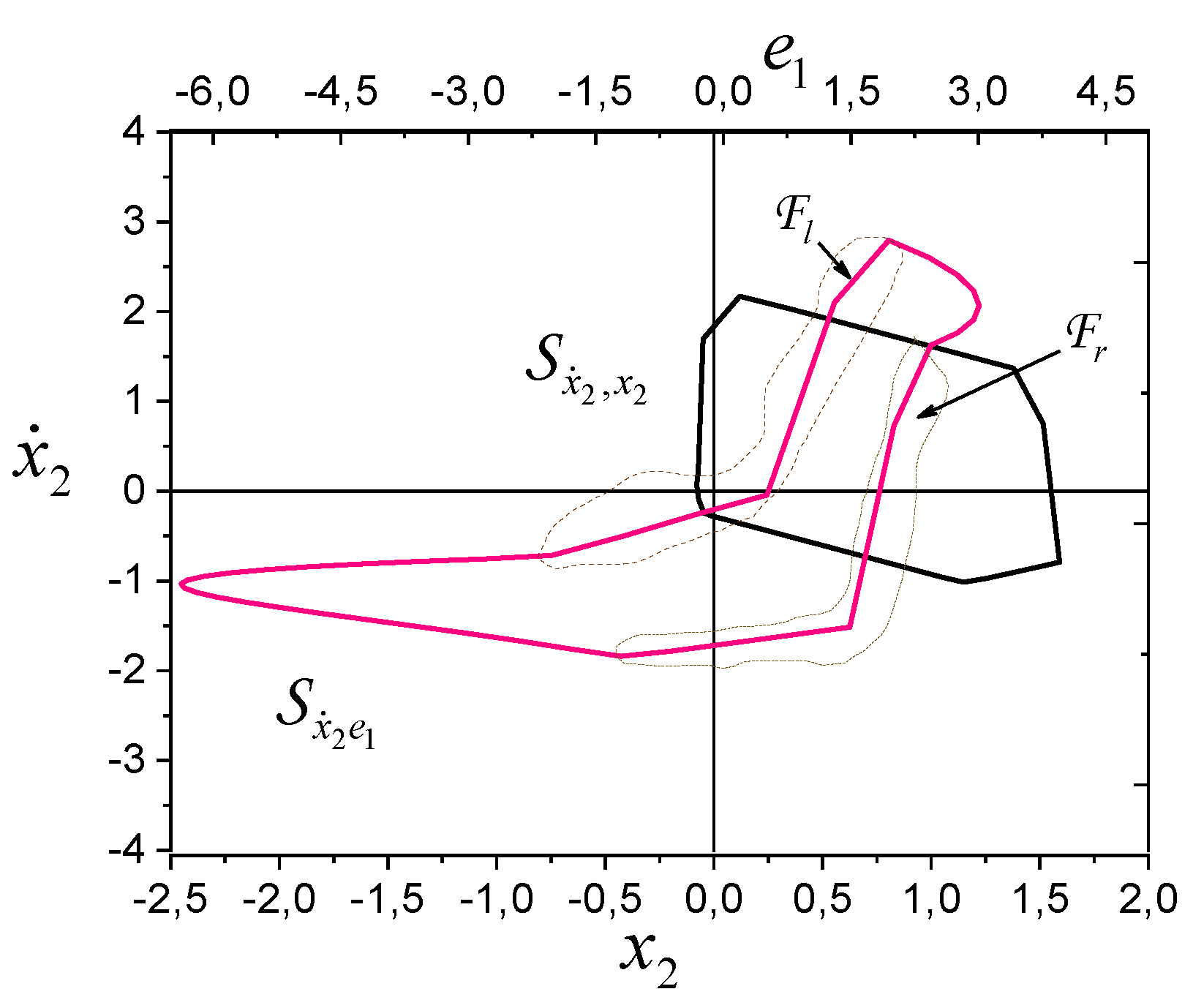
3. Consider the engine stabilization system with external feedback
where are amplifier parameters; is input; are engine parameters; are positive numbers; is a feedback coefficient.
System parameters (19), (20): , , , , , , , , , , , , . As the simulation showed, there are many synchronizing inputs for the system. But reducing the input frequency changes the response time of the nonlinear element. This complicates the identifiability analysis.
The phase portrait and the framework of the system (for steady state) show in Figure 5. Structures have an asymmetrical form. Since there is a closer relationship between and , then use the framework for analysis, where . We conclude about the asymmetry based on the right side analysis. Fragment is almost G2-homothetic to fragment (Figure 5). Therefore, the -framework is detectable and recoverable, and the system (19), (20) is -homothetic and -identifiable.
Remark 5. Feedbacks perform the signal adulteration. In this case, the choice has a certain problem. The system phase portrait can be used as an indicator of such an effect.
6. Conclusion
The identifiability problem of dynamical systems with nonsymmetric nonlinearities consider. We propose requirements for system input guaranteed an assessment of the nonlinear system structural identifiability. The input must be constantly excited and S-synchronizing. The problem solution based on the construction and analysis of virtual structures reflecting the nonlinear properties of the system. -homothety and structural identifiability conditions obtained for a system with nonsymmetric nonlinearities. The detectability and recoverability of virtual structures under uncertainty conditions proved. Conditions obtain under which a nonsymmetric nonlinearity can be a hypothetical symmetric nonlinearity.
References
- Shakiba, S. , Ourak M., Poorten E. V., Ayati M., Yousefi-Koma A. Modeling and compensation of asymmetric rate-dependent hysteresis of a miniature pneumatic artificial muscle-based catheter. Mechanical Systems and Signal Processing 2021, 154, 107532. [Google Scholar] [CrossRef]
- Hao, L. , Yang H., Sun Z., Xiang C., Xue B. Modeling and compensation control of asymmetric hysteresis in a pneumatic artificial muscle. J. Intell. Mater. Syst. Struct 2021, 28, 2769–2780. [Google Scholar] [CrossRef]
- Yang, H. , Zhang Y., Chen Y., Sun Y., Hao L. A novel learning adaptive hysteresis inverse compensator for pneumatic artificial muscles. Smart Mater. Struct 2020, 29, 015035. [Google Scholar] [CrossRef]
- Yang, H. , Chen Y., Sun Y., Hao L. A novel kriging-median inverse compensator for юmodeling and compensating asymmetric hysteresis of pneumatic artificial muscle. Smart Mater. Struct 2018, 27, 115019. [Google Scholar] [CrossRef]
- Song, J. , Der Kiureghian A. Generalized Bouc–Wen model for highly asymmetric hysteresis. Journal of Engineering Mechanics 2006, 6, 610–618. [Google Scholar] [CrossRef]
- Zhang, X. , Chen X., Zhu G., Su C.-Y. Output feedback adaptive motion control and its experimental verification for time-delay nonlinear systems with asymmetric hysteresis. IEEE Transactions on Industrial Electronics 2020, 67, 6824–6834. [Google Scholar] [CrossRef]
- Wei, Z. , Xiang, B. L., and Ting, R. X. Online Parameter Identification of the Asymmetrical Bouc-Wen Model for Piezoelectric Actuators. Precision Engineering 2014, 38, 921–927. [Google Scholar] [CrossRef]
- Wei, Z. , Wang D. Non-symmetrical Bouc–Wen model for piezoelectric ceramic actuators. Sensors and Actuators A: Physical 2012, 181, 51–60. [Google Scholar] [CrossRef]
- Brandhofer, S. , Myers C.R., Devitt S. J, Polian I. Multiplexed pseudo-deterministic photon source with asymmetric switching elements. arXiv, 2023; arXiv:2301.07258. [Google Scholar]
- Xie, S.-L. , Liu H.-T., Mei J.-P., Guo-Ying G. Modeling and compensation of asymmetric hysteresis for pneumatic artificial muscles with a modified generalized Prandtl–Ishlinskii model. Mechatronics 2018, 52, 49–57. [Google Scholar] [CrossRef]
- Aljanaideh, O. , Rakheja S., Chun-Yi Su. Experimental characterization and modeling of rate-dependent asymmetric hysteresis of magnetostrictive actuators. Smart Mater. Struct 2014, 23, 035002. [Google Scholar] [CrossRef]
- Hayashi, C. (1964) Nonlinear oscillations in physical systems. McGraw-hill Book Company.
- Popov, E.P. (1988) Theory of nonlinear automatic control and control systems. Nauka: Moscow.
- Zheng, W. , Zhang Z., Wang H. Adaptive state feedback control for nonlinear systems with multiple interval time-varying delays and non-symmetric dead-zone input: A Lyapunov-Krasovskii approach. Transactions of the Institute of Measurement and Control 2019, 41. [Google Scholar] [CrossRef]
- Du, C.; Yang, C.; Li, F.; Gui, W. A novel asynchronous control for artificial delayed Markovian jump systems via output feedback sliding mode approach. IEEE Transactions on Systems, Man, and Cybernetics: Systems 2019, 49, 364–374. [Google Scholar] [CrossRef]
- Karabutov, N.N. (2021) Introduction to the structural identifiability of nonlinear systems. URSS/LENAND: Мoscow.
- Karabutov, N.N. S-synchronization structural identifiability and identification of nonlinear dynamic systems. Mekhatronika, Avtomatizatsiya, Upravlenie 2020, 21, 323–336. [Google Scholar] [CrossRef]
- Kazakov, I.E. , Dostupov B.G. (1962) Statistical dynamics of nonlinear automatic systems. Fizmatgiz: Moscow.
- Furasov, V.D. (1977) Stability of motion, estimation and stabilization. Nauka: Moscow.
- Karabutov, N. (2017) Structural methods of design identification systems, In Nonlinearity problems, solutions and applications. Volume 1. Ed. L.A. Uvarova, A. B. Nadykto, A.V. Latyshev. Nova Science Publishers Inc: New York, 233-274.
- Karabutov, N. Structural identification of nonlinear dynamic systems. International journal of intelligent systems and applications 2015, 7, 1–11. [Google Scholar] [CrossRef]
- Hadamard, J. (1948) Lecons de geometrie elementaire. T. 2: Geometrie dans l'espace. Paris: Armand Colin & Cie.
Figure 1.
Phase portrait and structure .
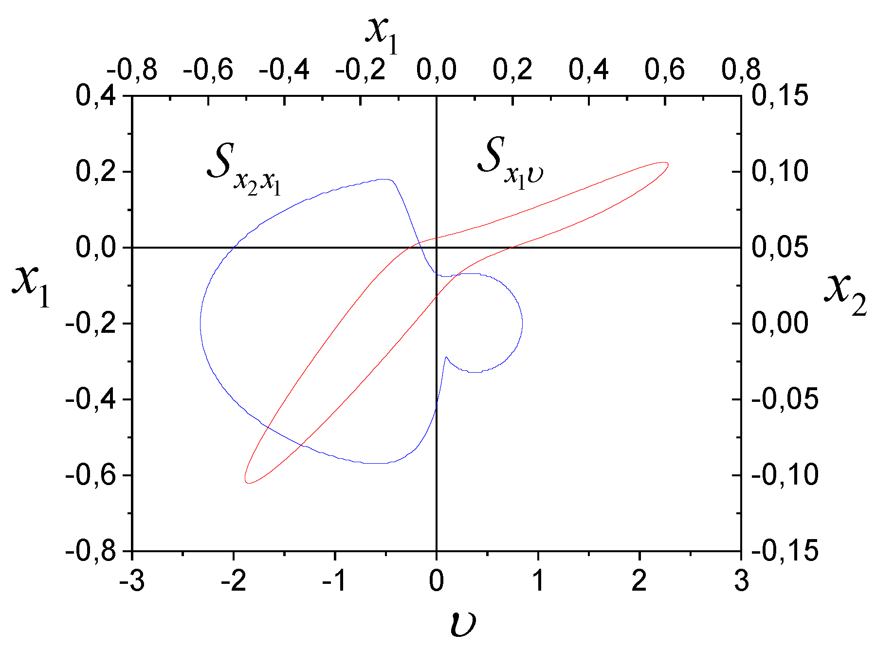
Figure 2.
Phase portrait of system (17), (18).
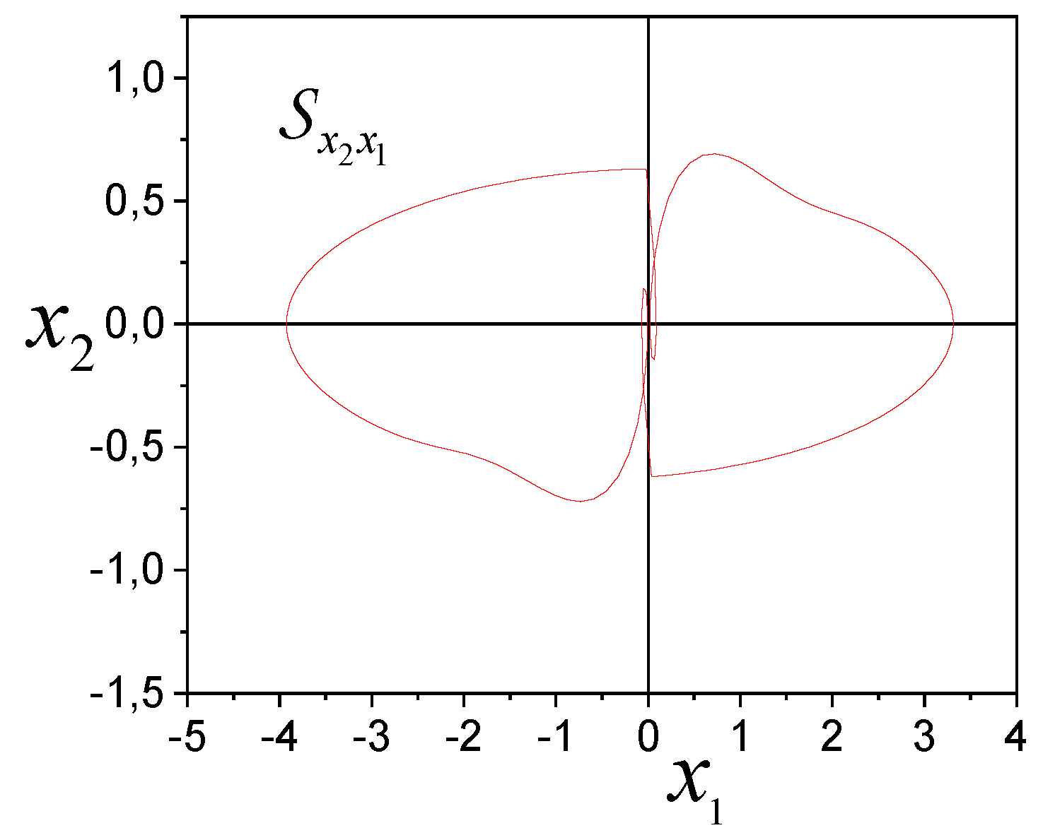
Figure 3.
Framework .
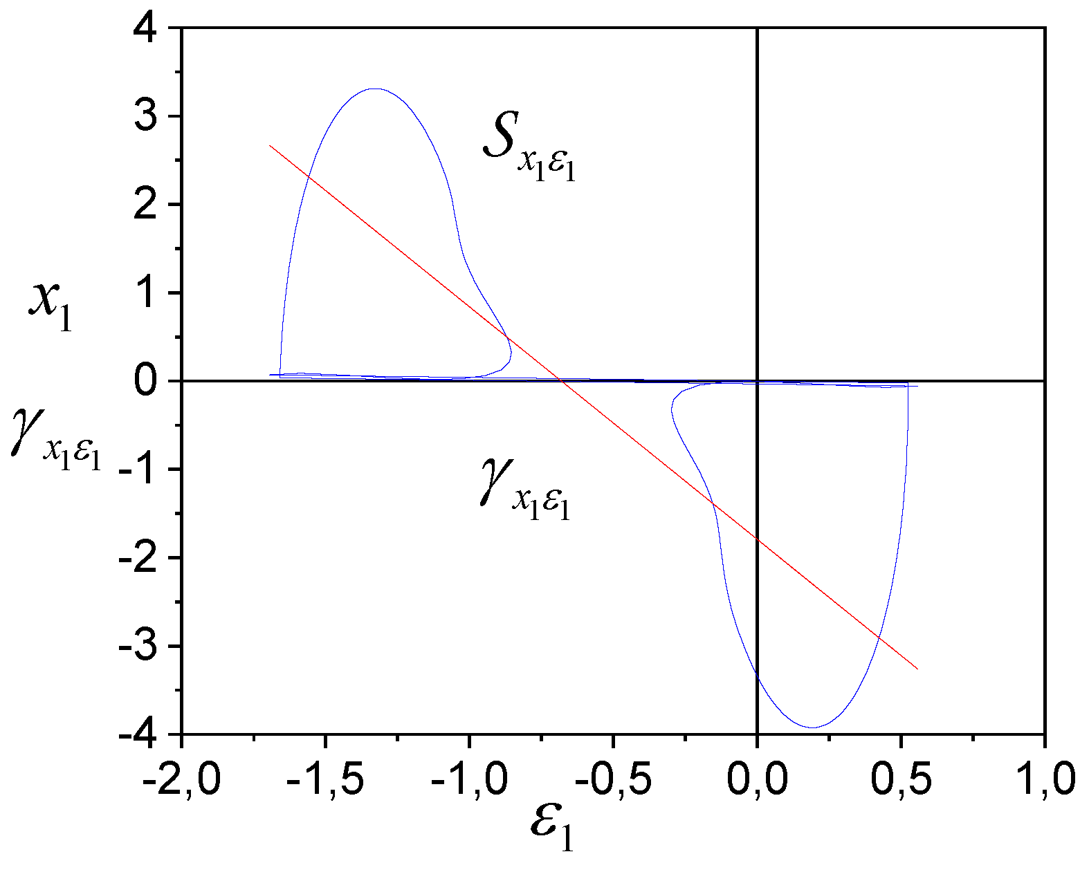
Figure 4.
Checking -structure -homothety.
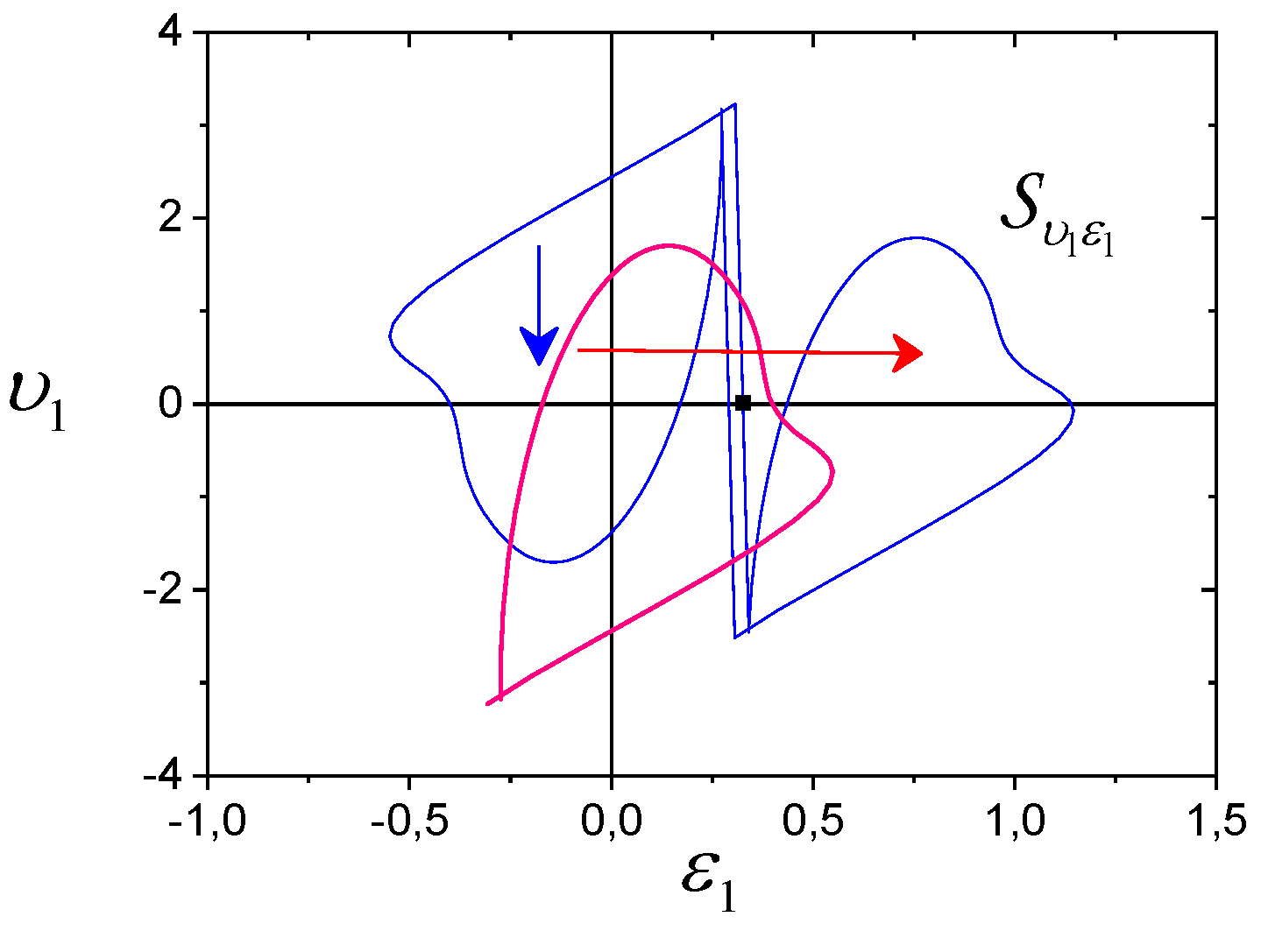
Figure 5.
Frameworks for system (19), (20).
Disclaimer/Publisher’s Note: The statements, opinions and data contained in all publications are solely those of the individual author(s) and contributor(s) and not of MDPI and/or the editor(s). MDPI and/or the editor(s) disclaim responsibility for any injury to people or property resulting from any ideas, methods, instructions or products referred to in the content. |
© 2023 by the authors. Licensee MDPI, Basel, Switzerland. This article is an open access article distributed under the terms and conditions of the Creative Commons Attribution (CC BY) license (http://creativecommons.org/licenses/by/4.0/).
Copyright: This open access article is published under a Creative Commons CC BY 4.0 license, which permit the free download, distribution, and reuse, provided that the author and preprint are cited in any reuse.


