
Submitted:
17 February 2025
Posted:
18 February 2025
You are already at the latest version
Abstract
The identifiability problem nonlinear decentralised systems (NDS) were not considered. Synthesis of mathematical models for NDS having a complex structure is an urgent problem. The presence of internal relationships and nonlinearities in NDS complicates the identifiability estimation. Therefore, models with uncertainty are used to design control systems for NDS. To describe the processes in NDS, it is necessary to apply adequate models based on verifying their identifiability. We propose an approach for assessing the local structural identifiability of nonlinear decentralised systems. Conditions of local parametric identifiability are obtained as functional constraints for parameters and nonlinearity.The effect of the constant excitation of experimental data on the S-synchronizability of DS is shown. The S-synchronizability condition fulfilment guarantees the structural identifiability estimate of DS with nonlinearity belonging to a certain sector. We introduce the S-congruence concept and propose a method for estimating the S-synchronizability of an input. Geometric structures and criteria are used to assess NDS identifiability. The simulation results are presented.
Keywords:
identifiability
; geometric structure
; decentralised system
; S-synchronizability
; constant excitation
; S-congruence
; quadratic coupling
; nonlinearity
1. Introduction
Increasing the requirements for the DS mathematical description requires solving the structural identifiability (SI) problem. A lot of attention is paid to SI issues. This is relevant for biological systems that are described by models with many parameters [1,2]. Various problems of SI are discussed in [3,4,5,6,7,8,9]. The identifiability problem is parametric, and its solution is based on ensuring the completeness (rank) of the information matrix. Its solution is based on Taylor series expansion [10], series generation method, similarity transformation [11] and differential algebra. In identification theory, this requirement is equivalent to the condition of constant excitation [5].
The parametric paradigm [11] as the main research in the identification is being transformed into nonlinear systems. The issues of parametric identifiability (PI) of nonlinear systems are considered in many works (see, for example, [12-15 et al.]). Sensitivity methods are used [12], conditions for local parametric identifiability are got based on experimental data [13] analysis. A study of approaches used to assess the identifiability of biological models is given in [14]. A critical analysis of the data requirements used in parametric identifiability problems is considered in [15]. The study of global, local, structural and practical identifiability is considered in [1, 5, etc.].
There are several interpretations of the structural identifiability concept. Various authors understand the SI as the possibility of an unambiguous estimation of system parameters. SI [16,17,18] is interpreted as the possibility of an unambiguous theoretical assessment of model parameters based on given data. In [19], SI is understood as the a priori identifiability (AI) of a model with the set structure, since identifiability properties are based on the transformation of the model equation (such transformations are aimed at the possibility of estimating model parameters, rather than choosing the model structure). Most of SI approaches are a priori method. The analysis of existing approaches to AI is given in [19,20]. In this paper, SI is understood as an opportunity to evaluate the DS structure.
The identifiability of decentralised systems (DS) has not been studied. In principle, DS is a multivariable system (MS), whose SI has been studied by various authors. The main difference between DS and MS is internal connections, which complicates the study of SI.
In this paper, we consider the SI problem of nonlinear decentralised systems. The concepts and definitions of parametric identifiability (PI) are given. We consider conditions of constant excitation and S-synchronizability, which guarantee the SI of the NDS. We study the PI of decentralised systems with nonlinearities satisfying the sector condition and obtain functional conditions that ensure local PI. Conditions for the relationship between subsystems that guarantee the identifiability of the nonlinear part of the DS are considered. Geometric structures that are the basis for SI analysis are presented. In the final part of the paper, we describe the approach used to estimate the structural identifiability of NDS. In the final part of the article, we consider the approach used to evaluate the NDS structural identifiability and present simulation results.
2. Problem Statement
Consider a system comprising interconnected subsystems
where , are vectors of the state and output of -subsystem, is control, , . Coefficients of the matrices are unknown, . The matrix reflects the mutual influence of the subsystem. consider the nonlinear state of the -subsystem, and is Hurwitz matrix (stable).
Assumption 1. belongs to the class
and satisfies the quadratic condition
Information set for subsystems Si
Mathematical model for
where is Hurwitz matrix with known parameters (reference model); , are tuning matrices of corresponding dimensions, is a priori given nonlinear vector function.
Problem: based on the analysis , determine the SI conditions for the -subsystem.
3. Some Concepts and Definitions
Consider a dynamic system
where is state vector, is input vector (control), is output, is the initial condition, is vector of unknown parameters.
Definition 1 [21]. The parameter is structurally globally identifiable if for almost any
Definition 2 [21]. Let there be a neighbourhood such that
Then is structurally locally identifiable for any .
If the neighbourhood of does not exist, then the parameter is called structurally locally unidentifiable.
Definition 3 [21]. The model structure is globally identifiable at point if
where is a connected open subset of parameters.
Fulfilment of definition 3 conditions guarantees the identifiability of the model at the point.
4. Condition of Constant Excitation and S-Synchronizability
A priori identifiability is based on the analysis of rank conditions for the information matrix. In adaptive systems, conditions based on the constant excitation (CE) of set elements are used to analyse properties of the identification system.
Definition 4. The vector is continuously excited if
where is the identity ma, are positive numbers, .
We will write about the CE condition as . If condition (5) for is not satisfied, then we will write or
Since DS (1) is nonlinear, then we represent condition (5) as
where is the set of frequencies for ; is the set of acceptable frequencies for , guaranteeing S-synchronizability. Next, we will denote the CE property as , assuming that it guarantees .
The equation for the -subsystem identification error
where are parametric residuals.
Definition 5. The input will be called S-synchronising and written if it reflects all the nonlinear properties of the -subsystem.
5. PI Conditions
We consider the DS identifiability based on analysis .. This is practical identifiability.
Assumption 2. Let 1) ; 2) .
Definition 6 [22]. Let assumption 2 hold. Then the pair is called fully recoverable, and the -subsystem is fully recoverable.
Definition 7 [22]. Let the pair be fully recoverable. Then subsystem will be locally parametrically identifiable on the set , if estimates of the model (4) parameters belong to some limited region of the parametric space .
We will consider the results [23], which will be used.
Lemma 1. If the nonlinearity belongs to the class , then
where , .
Lemma 2. If the conditions of Lemma 1 are satisfied, then
where , , , .
Consider the system (6) and the Lyapunov function (LF) , where is the positive symmetric matrix. Let where is the matrix norm, is the trace of the matrix.
The following conditions for the local identifiability of subsystem are valid in the parametric space. They are a modification of Theorem 1 [23].
Theorem 1. Let 1) ; 2) , ; 3) Lemma 1, 2 conditions of are fulfilled for ; 4) assumption 2 holds. Then the system (1) is locally parametrically identifiable on the set if
where , is the minimum eigenvalue of the matrix , , , is the positive symmetric matrix, , , , .
Corollary of Theorem 1. Let the conditions of Theorem 1 be fulfilled. Then the nonlinearity is locally structurally identifiable in the sector
If
where .
The proof of the corollary from Theorem 1 is given in Appendix A.
We see that the -subsystem will be parametrically identifiable if the nonlinearity dominates on the effects of the subsystem.
The corollary from Theorem 1 gives the conditions under which the local structural identifiability is possible for the nonlinear part of subsystem in sector .
Definition 8. If conditions (8), (9) are fulfilled, then subsystem is locally structurally identifiable at the parametric level.
Remark 1. Theorem 1 provides conditions for the local SI of the system R1 in the form of estimates for the model (2) parameters belonging to the limited region of parametric space.
Consider the input-output information set
For subsystem , we get the representation [23]
where , , # is the sign of the pseudo-conversion of the matrix.
Model for the system (10)
and the equation for the error
where , , . The matrix is selected to ensure the stability of the identification process.
Definition 9. If the conditions of assumption 2 are fulfilled and the pair is fully recoverable and the pair is stabilised, then subsystem (10) is called fully recoverable.
Definition 10. Let assumption 2 hold. Then 1) the system (10) is detectable if the subspace of non-recoverable states is contained in the subspace of stable states; 2) the pair is detectable.
Introduce the error and ФЛ .
Theorem 2. Le: 1) ; 2) , ; 3) Lemma 1, 2 conditions of are fulfilled for ; 4) the system (10) is observable, recoverable, and stabilised. Then the system (10) is locally structurally parametrically identifiable on the set G2 if
where
Theorem 2 is proved similarly to Theorem 1.
So, conditions (12), (13) guarantee the local parametric identifiability of the system (1) in the output space.
Remark 2. In Theorems 1 and 2, the concept of the "structurally identifiable system" is understood in a parametric sense. This follows from estimates for nonlinearity obtained in Lemmas 1 and 2. The concept of structural refers to non-linearity, which must belong to class and satisfy the functional constraint (13).
Consider the SI problem. Apply the approach based on the special class analysis of geometric frameworks [24].
6. Geometric Frameworks
Consider the system . Let and is th element of the output vector. Calculate the derivative and denote it as . Construct a phase portrait for the -system in the space . Consider structures described by the functions . Introduce the model for :
on the set and calculate the error , where are numbers determined using the least squares method.
Define the structures and described by the mappings and .
Remark 3. The model (14) structure can change. The number of independent variables on the right-hand side (14) depends on the properties of the subsystem . The choice of the model (14) structure is based on the iterative immersion method [24].
For the system , we construct the geometric framework (GF) described by the function . Then, the subsystem can be represented as:
where is a variable describing the general solution of the system (1); is a limited disturbance that appears as a result of the allocation of the variable 2.
7. SI of Subsystem
Let and .
Definition 10 [24]. The input is an S-synchronising for system (1) if the domain of the structure has a maximum diameter on the set , where is multiple synchronization inputs having the CE property ; is the set of acceptable inputs for the -subsystem.
If the input is S-synchronizing, then we will write . We understand the diameter as the maximum distance between two points .
Consider a system and frameworks , and .
Definition 11. Frameworks and are S-congruent if their structural features are similar.
Definition 12. If , and are S-congruent, then the input is S-synchronising and guarantees the S-synchronizability of the system .
Definition 12 provides a criterion for selecting the required input having the specified properties and the property is valid for it.
As shown in [25], () guarantees the SI of NDS, where the index is a sign of identifiability.
There may be some subset () whose elements have the property of S-synchronizability. The structure with a diameter corresponds to each . Since , the diameters will have the -optimality property [25].
Let the hypothetical framework (structure ) of the system have diameter . The reference framework is the structure , reflecting all the properties of the function .
Designate the diameter as . exists for the -system having the S-synchronising input.
If , then , where , is a proximity sign. The elements of the subset have the property
Definition 13 [25]. The framework has the -optimality property on the set if there exists such that , , where is cardinality of set .
Definition 14 [25]. If the subset of inputs () the elements of which are and their corresponding frameworks have the of -optimality property, then frameworks are structurally indistinguishable on sets and .
It follows from definitions 13 and 14 that if there is the set , then the -identifiability (SI) estimate is obtained for any input .
Definition 15 [25]. Frameworks that do not have the -optimality property are locally structurally unidentifiable (SNI) on the set .
Remark 4. The framework , which is SNI on the set , defines the class . Here , belongs to the insignificant structures for which the -optimality condition is not fulfilled.
Definition 16. Frameworks defining the class for the function and having the -optimality property are locally structurally identifiable on the set .
Notation:
- (a)
- is the framework , which has the -optimality property;
- (b)
- is a locally structurally identifiable framework .
Let , where are the left and right fragments . The fragments are determined on areas with diameters . Then the system is locally structurally identifiable or -identifiable and if
where .
Remark 4. We have considered the case of non-linearities belonging to the class . has a set of non-linearities, which are both symmetric and non-symmetric. If is non-symmetric and , then we use the approach [26] to estimate SI. Here, the SI assessment is reduced to ensuring -identifiability.
Remark 5. Structural identification depends on the connections between subsystems. These connections must be stable and satisfy the corollary of Theorem 1. This condition guarantees the identifiability of the nonlinear part of the -subsystem at the parametric level. This approach allows you to localise the nonlinearity to evaluate the SI.
Definition 16. NDS is locally structurally identifiable if conditions of Theorems 1, 2 are fulfilled, and the nonlinear part is SI.
8. Simulation Results
1. Consider the system
where and are the state vector and output of the subsystem ; are input (control)); is saturation function; is sign function; is subsystem output. System parameters (18): , , , , , , . Inputs are sinusoidal.
For the -subsystem, the phase portrait is shown in Figure 1. The processes are nonlinear. There is a relationship between and (the determination coefficient is 75%), which affects the properties of the subsystem (see Figure 1).
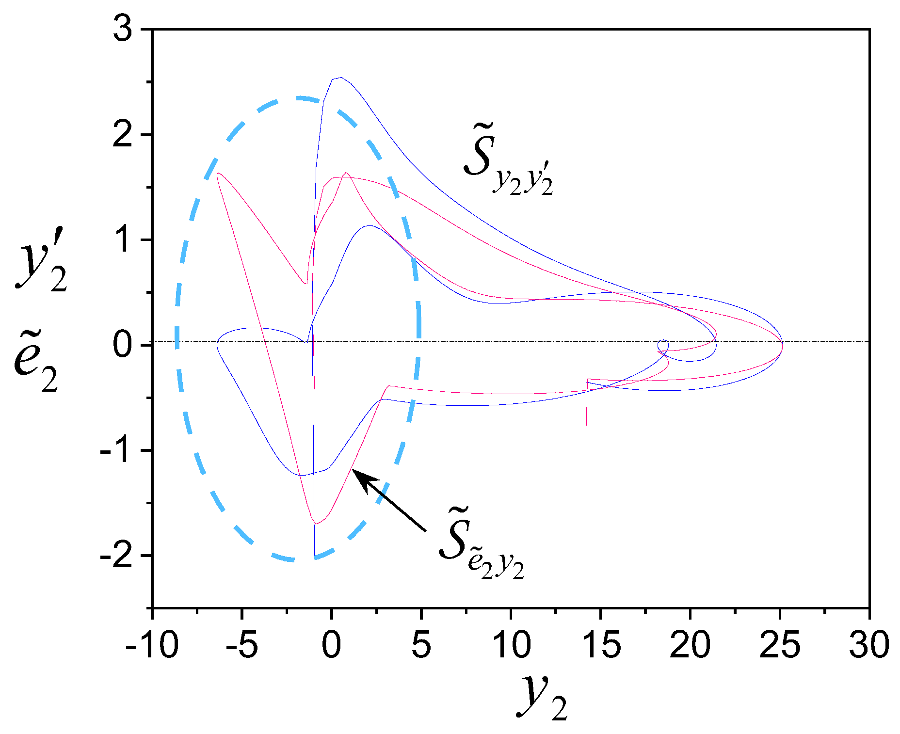
The results of the evaluation of the S-congruence for subsystems are presented in Figure 2 and Figure 3, which show phase portraits and frameworks.
We see the frameworks are S-congruent, and the inputs (controls) are S-synchronising.
Remark 5. In the space , the subsystem has the representation
where , ,, are coefficients; ,
The application of filters (20) changes the original frequency spectrum of the system (18). Here, the S-congruence estimation procedure also works, but the set of inputs must change. This is confirmed by the simulation results.
The structure is shown in Figure 4. It is obtained as follows. Since there is the relationship , the iterative immersion method is used to obtain .
To exclude the effect of on , we synthesized a model
The variable is used to construct the model (14), which has the form for the system (18)
Apply (22) and get the structure described by the function , where
The average diameters of fragments are equal . If we put in (17), then we get that the system is -identifiable. It follows from Figure 4 that the nonlinearity of is a function of saturation.
So, the subsystem of the -subsystem (18) is locally structurally identifiable.
Consider the subsystem . Data analysis has shown that there is an impact of on . Therefore, we apply the iterative immersion method and use
as the model (14), and calculate the error . Next, the geometric framework (Figure 5) described by the function is definable. The results are shown in Figure 5. We see (a) subsystem is SI and contains non-linearity belonging to the class of sign functions; (b) structures and are S-congruent.
Remark 6. If the S-synchronizability conditions are not fulfilment, then DS may be unidentifiable.
2. Consider the system
where are state vectors of the subsystem ; is are; are inputs (control); ; . System parameters (23): , , , , , , , , . Inputs are sinusoidal.
The simulation results confirm the S-synchronizability of the inputs. We apply the D2 model
to construct the structure and calculate the residual . The structure , described by the function , and the phase portrait are shown in Figure 6. We see frameworks and are S-congruent, and subsystem is structurally identifiable. The framework represents the nonlinearity .
Consider the subsystem . The phase portrait and the structure are shown in Figure 7. We see that subsystem is structurally identifiable, and the framework coincides with the function . The analysis showed that is influenced by the variable . Therefore, apply the model:
which is the basis for calculating the residual and constructing the -structure. The oval (Figure 7) allocates the area that contains the -fragment corresponding to .
So, simulation results confirm the effectiveness of the proposed approach to SI. The of the model structure (14) choice is the main problem of this method. The model identification depends on the DS type, experimental data properties, and the intuition of the researcher. Using the iterative immersion method solves this problem. The effectiveness of this method is showed by examples. The examples show it is difficult to propose a general approach to SI estimate. This is because of the peculiarities of the nonlinear system. Therefore, the DS detailed analysis and the results of data processing are the basis for deciding about SI.
9. Conclusions
An approach is proposed for assessing the local structural identifiability of a nonlinear decentralised system. The relationship is shown between the excitation constancy of the experimental data and the S-synchronizability, which guarantees the possibility of SI estimating for the NDS. We have obtained the local SI condition at the parametric level for subsystems, satisfying the quadratic condition for nonlinearity. The S-congruence concept is introduced, and the method is proposed, ensuring S-synchronizability of the input. Geometric structures and criteria are considered for estimating the structural identifiability of NDS.
Appendix
Corollary proof from Theorem 1. According to Theorem 1, NDS is locally parametrically identifiable if
where . From Lemmas 1 and 2, we get:
Therefore
where
From the stability condition, we obtain , therefore . ■
References
- Saccomani M. P. Structural vs practical identifiability in system biology. IWBBIO 2013. Proceedings. Granada, 18-20 March, 2013;305-313.
- Villaverde A., Barreiro A., Papachristodoulou A. Structural identifiability of dynamic systems biology models. PLOS Computational Biology. 2016;12(10); 1–22. [CrossRef]
- Vanelli M., Hendrickx J. M. Local identifiability of networks with nonlinear node dynamics. arXiv:2412.08472v2 [math.OC] 31 Dec 2024.
- Zhong Y. D., Leonard N. E. A continuous threshold model of cascade dynamics. In 2019 IEEE 58th Conference on Decision and Control (CDC), IEEE, 2019, pp. 1704–1709.
- Vizuete R., Hendrickx J. M. Nonlinear network identifiability with full excitations, arXiv preprint arXiv:2405.07636, 2024.
- Legat A., Hendrickx J. M. Path-based conditions for local network identifiability. In 2021 60th IEEE Conference on Decision and Control (CDC), IEEE, 2021;3024–3029.
- Zhong Y. D., Leonard N. E.A continuous threshold model of cascade dynamics. In 2019 IEEE 58th Conference on Decision and Control (CDC), 2019;1704–1709.
- Lekamalage A. S. Identifiability of linear threshold decision making dynamics, 2024.
- Raue A., Becker V., Klingmüller U., Timmer J. Identifiability and observability analysis for experimental design in nonlinear dynamical models. Chaos, 2010;20(4); 045105. [CrossRef]
- Chis O.-T., Banga J. R., Balsa-Canto E. Structural identifiability of systems biology models: a critical comparison of methods. PLoS ONE, 2011;6(4);1-16. [CrossRef]
- Vajda S, Godfrey K, Rabitz H. Similarity transformation approach to identifiability analysis of nonlinear compartmental models. Mathematical Biosciences, 1989;93;217–248. [CrossRef]
- Stigter J. D., Peeters R. L. M. On a geometric approach to the structural identifiability problem and its application in a water quality case study. Proceedings of the european control conference 2007 Kos, Greece, July 2-5, 2007, 2007; 3450-3456.
- Handbook on the theory of automatic control / Edited by A. A. Krasovsky. Moscow: Nauka, 1987.
- Chis O.-T., Banga J. R., Balsa-Canto E. Structural identifiability of systems biology models: a critical comparison of methods. PLoS ONE, 2011;6(4);1-16. [CrossRef]
- Guillaumea H. A., Jakeman J. D., Marsili-Libellid S. et al. Introductory overview of identifiability analysis: A guide to evaluating whether you have the right type of data for your modeling purpose. Environmental Modeling and Software, 2019;119; 418–432.
- Conrad J. R., Eisenberg M. C. Examining the impact of forcing function inputs on structural identifiability. arXiv:2407.02771v1 [q-bio.QM] 3 Jul 2024.
- Weerts H.H.M., Dankers A. G., Van den Hof P. M. J. Identifiability in dynamic network identification. Preprints of the 17th IFAC Symposium on System Identification Beijing International Convention Center October. Beijing, China, 2015;19-21,.
- Verdière N. Identifiability in networks of nonlinear dynamical systems with linear and/or nonlinear couplings. Franklin Open, 2024, 9, 100195. [CrossRef]
- Anstett-Collin F., Denis-Vidal L., Millérioux G. A priori identifiability: An overview of definitions and approaches. Annual Reviews in Control, 2020;50;139-149. [CrossRef]
- Karabutov N. N. Introduction to the structural identifiability of nonlinear systems. Moscow: URSS/Lenand, 2021.
- Ljung L. System Identification: Theory for the User. Prentice Hall, 1999.
- Kwakernaak, H., Sivan R. Linear optimal control systems. New York, Wiley Interscience, 1975. [CrossRef]
- Karabutov N. Identification of decentralised control systems. Preprints-143582. https://www.preprints.org/manuscript/202412.1808/v1. [CrossRef]
- Karabutov N. N. S-synchronization Structural Identifiability and Identification of Nonlinear Dynamic Systems. Mekhatronika, Avtomatizatsiya, Upravlenie, 2020;21(6); 323-336.
- Karabutov N. Structural identifiability of systems with multiple nonlinearities. Contemporary Mathematics, 2021;2(2);103-172. [CrossRef]
- Karabutov N.N. Structural Identifiability Evaluation of System with Nonsymmetric Nonlinearities. Mekhatronika, Avtomatizatsiya, Upravlenie,2024;25(2);55-64. [CrossRef]
Figure 1.
Phase portrait of the subsystem .
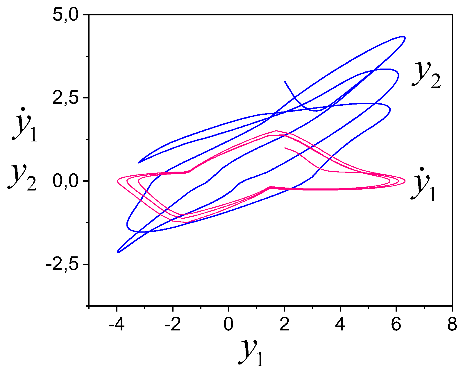
Figure 2.
S-congruence estimation for the subsystem .
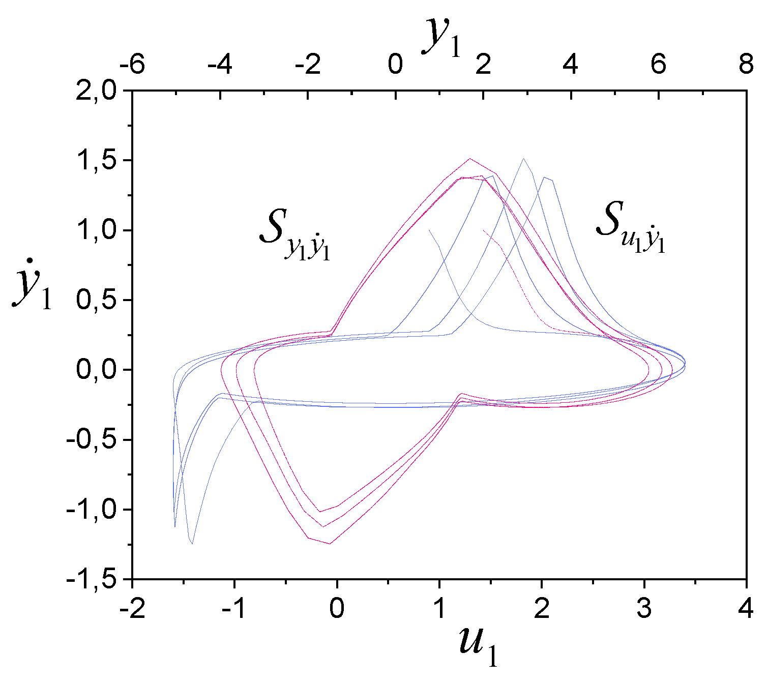
Figure 3.
S-congruence estimation for the subsystem .
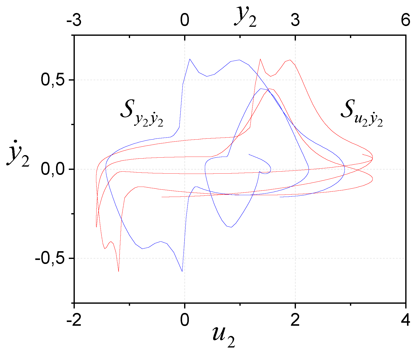
Figure 4.
Structure for the subsystem .
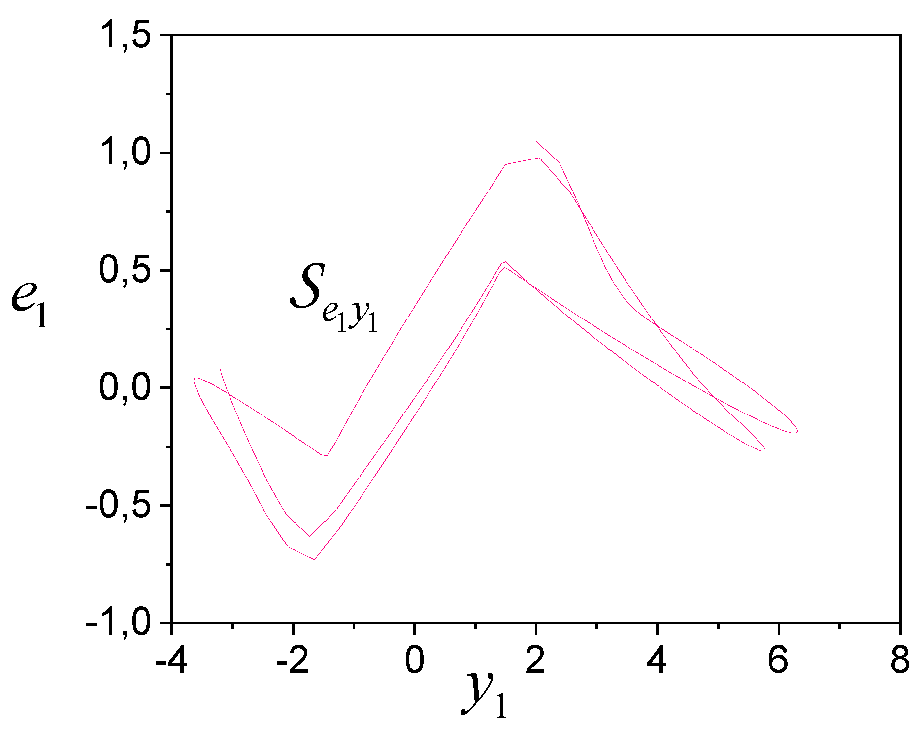
Figure 5.
Structural identifiability evaluation of subsystem .
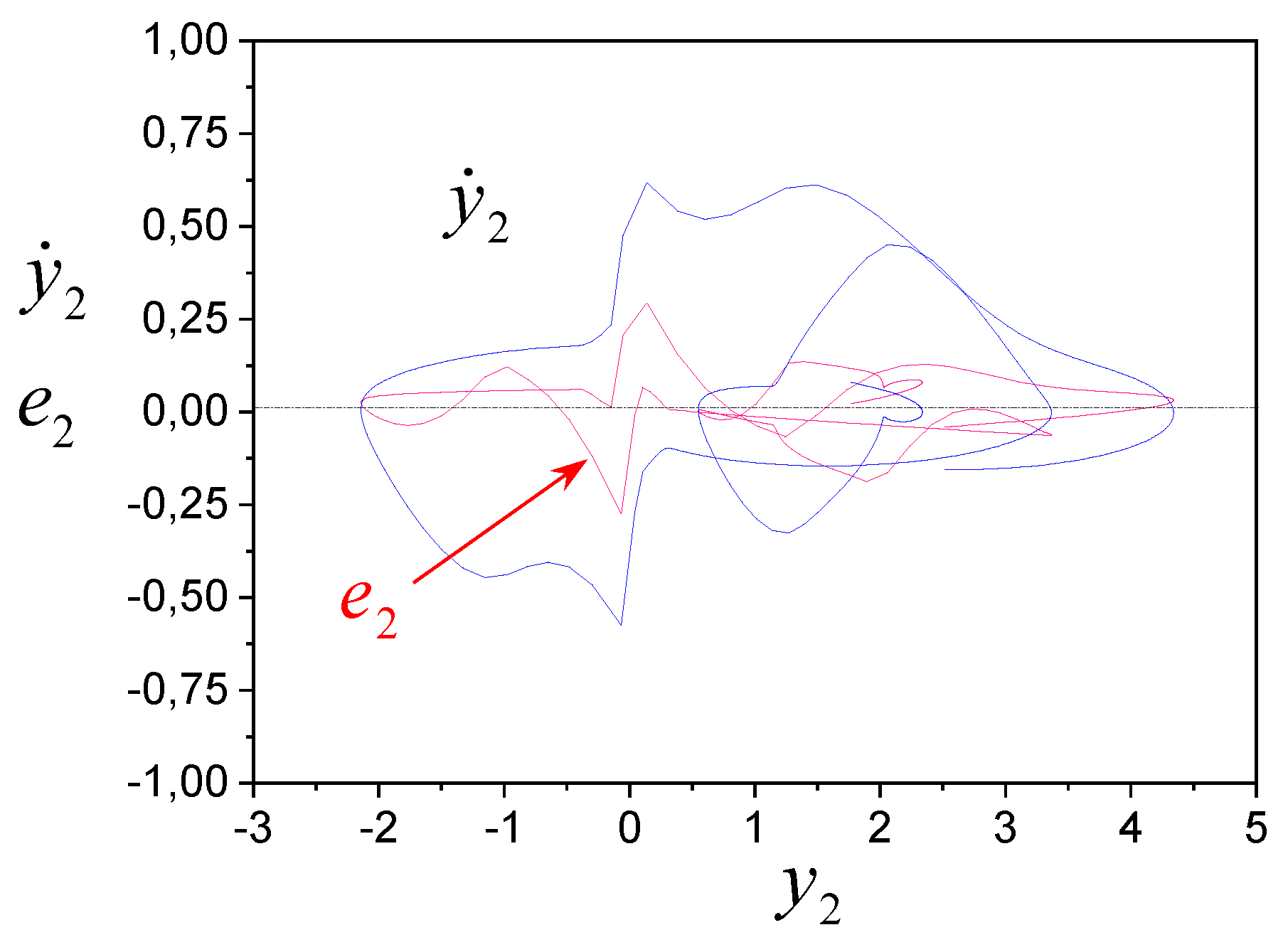
Figure 6.
SI evaluation of subsystem .
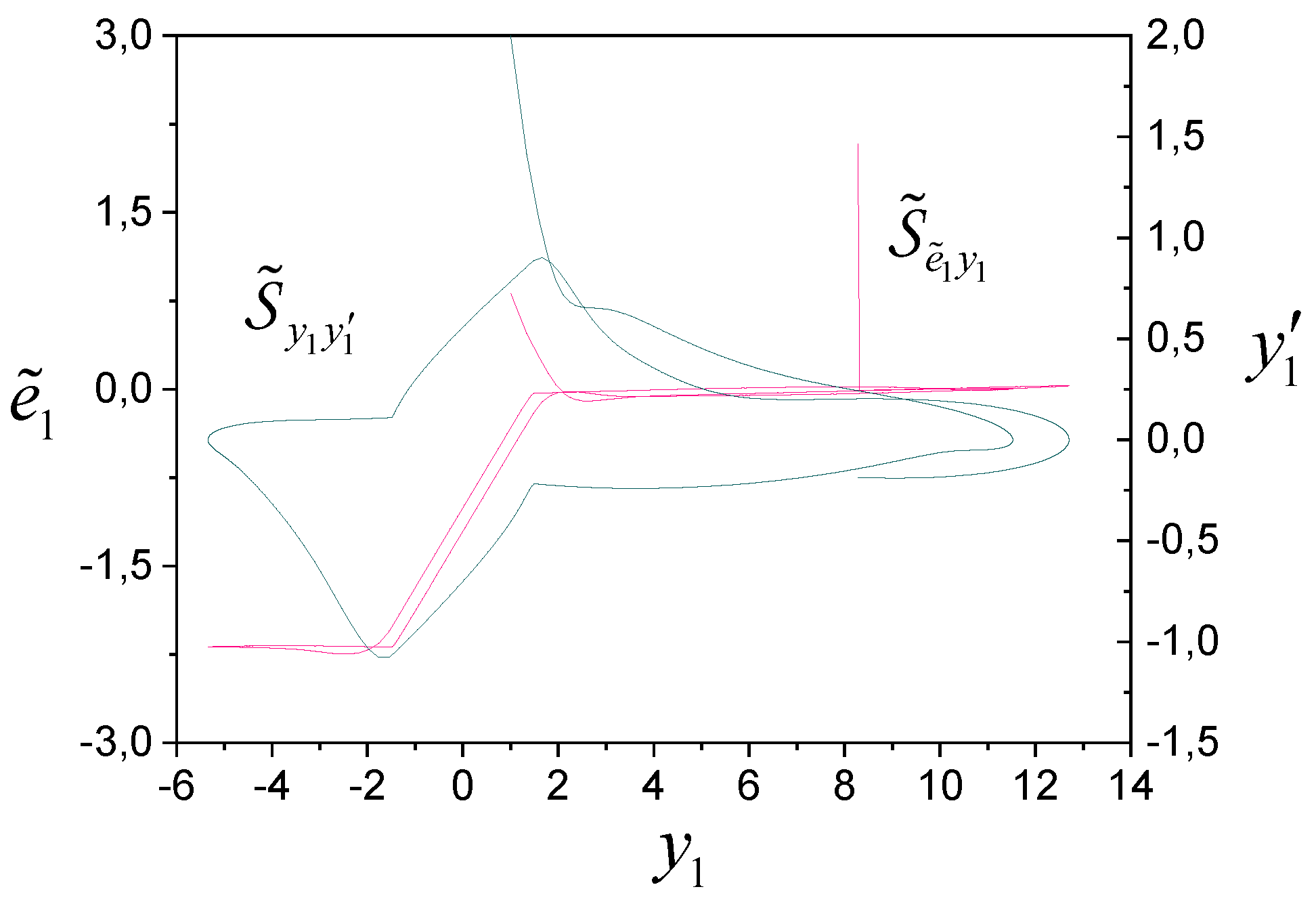
Figure 7.
SI evaluation of subsystem .
Disclaimer/Publisher’s Note: The statements, opinions and data contained in all publications are solely those of the individual author(s) and contributor(s) and not of MDPI and/or the editor(s). MDPI and/or the editor(s) disclaim responsibility for any injury to people or property resulting from any ideas, methods, instructions or products referred to in the content. |
© 2025 by the authors. Licensee MDPI, Basel, Switzerland. This article is an open access article distributed under the terms and conditions of the Creative Commons Attribution (CC BY) license (http://creativecommons.org/licenses/by/4.0/).
Copyright: This open access article is published under a Creative Commons CC BY 4.0 license, which permit the free download, distribution, and reuse, provided that the author and preprint are cited in any reuse.


