A Transverse Hamiltonian Approach to Infinitesimal Perturbation Analysis of Quantum Stochastic Systems

1. Introduction

In comparison with classical mechanics which considers macroscopic objects both in deterministic and stochastic settings, quantum mechanics, concerned with physical phenomena at atomic and subatomic scales, inherently incorporates randomness. In particular, the squared absolute value of the wave function of a quantum mechanical particle is interpreted as a probability density function, mixed quantum states are built of pure ones using randomisation, and the latter is also present in the model of quantum measurement [39,51]. However, in contrast to scalar-valued classical probability measures [41], quantum probability describes statistical properties of quantum variables by using quantum states in the form of density operators [16,30] on the same Hilbert space where those variables act as linear operators.

The noncommutativity and canonical commutation structures, coming from the operator-valued nature of quantum variables and quantum states, give rise to specific features of quantum probability such as the absence of a classical joint probability distribution and conditional expectations for a set of noncommuting quantum variables (whereas an individual self-adjoint operator has a well-defined marginal distribution). Furthermore, since the microscopic realm is less amenable to manipulation by conventional macroscopic tools (unlike, for example, the coin tossing as a manageable “random number generator” for thought and practical experiments in classical probability theory), its natural time evolution makes statistical properties of quantum systems particularly tied to their dynamics. While an isolated quantum system undergoes a reversible evolution (according to a one-parameter unitary group generated by the system Hamiltonian), a more realistic open dynamics scenario [6] involves interaction of the system with its environment which can include other quantum or classical systems, measuring devices and external quantum fields (quantised electromagnetic radiation).

The interaction of an open quantum system with its surroundings is accompanied by energy exchange between the subsystems and gives rise to dissipative effects. This provides a way to influence statistical and dynamic properties of such systems by arranging them into quantum networks [14] and varying the energy and coupling parameters of the resulting interconnections, which can consist of a quantum plant coupled in a measurement-based or coherent (that is, measurement-free) fashion to a controller or observer. This paradigm is used in quantum control [3,5,8] which develops systematic methods for achieving stability, robustness with respect to unmodelled dynamics, and optimality in the sense of relevant performance criteria for quantum systems and their applications, for example, in quantum optics [11,50] and quantum information processing [32].

An important part in these developments belongs to quantum filtering, which, similarly to its classical predecessor (see for example, [23,28]), is concerned with mean square optimal real time estimation of the internal variables of the quantum plant using a measurement-based quantum Kalman filter [2,4,9] or a qualitatively different coherent quantum observer [31,45]. The latter does not process classical observations and, in contrast to the classical filters, does not compute the conditional expectations of the plant variables (this conditioning and related Bayesian approaches are not applicable in the noncommutative quantum case as mentioned above). Instead, the coherent quantum filter is driven by the output quantum fields of the plant so as to produce a quantum process, whose performance, as an estimator of the plant variables, can be optimised in the sense of minimising the mean square value of the “estimation error” by varying the parameters of the Hamiltonian and coupling operators of the filter.

The optimisation problems, arising in coherent quantum filtering and control (with the latter considering more complicated feedback interconnections of a quantum plant and a quantum controller) involve physical realisability (PR) constraints [22,40] which originate from the canonical commutation structures of quantum dynamic variables, the energetics of open quantum systems, and unitarity in the augmented system-environment evolution. These features of open quantum dynamics are incorporated in the Hudson-Parthasarathy quantum stochastic calculus [19,35] (see also [15]) which is often employed as a unified modelling framework in quantum filtering and control. In this approach, the external fields at the input of a quantum system of interest are represented by a multichannel quantum Wiener process with noncommuting components, which act on a symmetric Fock space and drive the quantum stochastic differential equation (QSDE) governing the system dynamics. In contrast to the classical SDEs with a standard Wiener process [24], the QSDE reflects the unitarity of the augmented system-field evolution, and its drift and dispersion terms (as well as the generator of Markovian quantum dynamics) are specified by the Hamiltonian and coupling operators. These operators (together with a scattering matrix representing the photon exchange between the fields [35]) describe the energetics of the quantum system and its interaction with the environment and are usually functions (for example, polynomials or Weyl quantization integrals [10]) of the system variables. A particular form of this dependence and the commutation structure of the system variables affect tractability of the quantum system.

In particular, a quadratic dependence of the system Hamiltonian and a linear dependence of the system-field coupling operators on the quantum mechanical position-momentum variables [29] lead to linear QSDEs for open quantum harmonic oscillators (OQHOs) [9,11] which play the role of building blocks in linear quantum control theory [8,22,34,38,54,55]. The dynamics of such systems are relatively well understood and are similar to the classical linear SDEs in a number of respects, including the preservation of Gaussian nature of quantum states [20,36] in the case of vacuum input fields. However, the coherent quantum analogue [33] of the classical linear-quadratic-Gaussian (LQG) control problem [1,25] for OQHOs is complicated by the above mentioned PR constraints on the state-space matrices of the quantum controller and by the impossibility to take advantage of the classical estimation-actuation separation principle and classical conditional expectations with their variational properties [28].

One of the existing approaches to the coherent quantum LQG (CQLQG) control and coherent quantum filtering (CQF) problems employs the Frechet derivatives of the mean square cost (with respect to the state-space matrices subject to the PR constraints) for obtaining the optimality conditions [44,45] and for the numerical optimization [42]. This approach takes into account the quantum nature of the underlying problem only through the PR constraints, being “classical” in all other respects, which has its own advantages from the viewpoint of well-developed conventional optimization methods. However, a disadvantage of this approach is that it is limited to certain parametric classes of linear controllers and observers. In particular, the resulting optimality conditions do not provide information on whether nonlinear quantum controllers or observers can outperform the linear ones for linear quantum plants. For this reason, the coherent quantum control and filtering problems require novel variational methods for their solution, which would be able to operate with sensitivity of the system dynamics and relevant cost functionals to perturbations over wider classes of the Hamiltonian and coupling operators in a “coordinate-free” fashion.

To this end, the present paper (some of its results were briefly announced in [48]) outlines a fully quantum variational method which allows the sensitivity of the internal and output variables of a nonlinear quantum stochastic system to be investigated with respect to arbitrary (that is, not only linear-quadratic) perturbations of the Hamiltonian and coupling operators. This approach is based on using a transverse Hamiltonian, defined as an auxiliary time-varying self-adjoint operator which encodes the propagation of such perturbations through the unitary system-field evolution. This leads to an infinitesimal perturbation formula for quantum averaged performance criteria (such as the mean square cost functional) which is applicable to the development of optimality conditions in coherent quantum control and filtering problems over larger classes of controllers and observers. In particular, this approach allows the sensitivity of OQHOs with quadratic performance criteria to be studied with respect to general perturbations of the Hamiltonian and coupling operators. In fact, the transverse Hamiltonian method has already been employed in [47] in order to establish local sufficiency of linear observers in the mean square optimal CQF problem [45] for linear quantum systems with respect to varying the Hamiltonian and coupling operators of the observer along linear combinations of the Weyl operators [10]. Note that our approach is different from [13] which develops a quantum Hamilton-Jacobi-Bellman principle (for the density operator instead of the dynamic variables) in a measurement-based quantum feedback control problem. We also mention a parallel between the perturbation analysis, discussed in the present paper, and the fluctuation-dissipation theorem [26].

The paper is organised as follows. Section 2 specifies the class of quantum stochastic systems under consideration. Section 3 discusses sensitivity of the internal and output variables of OQHOs to parametric perturbations within the families of quadratic system Hamiltonians and linear system-field coupling operators. Section 4 returns to general QSDEs and introduces the transverse Hamiltonian associated with arbitrary perturbations of the Hamiltonian and coupling operators of the system. The transverse Hamiltonian is used in Section 5 for infinitesimal perturbation analysis of system operators. Section 6 extends the transverse Hamiltonian method to quantum averaged performance criteria. Section 7 applies this approach to a mean square optimal CQF problem. Section 8 makes concluding remarks.

We use the following principal notation in the paper. Denoted by $[A,B]:=AB-BA$ is the commutator of linear operators A, B, with ${\mathrm{ad}}_A(·):=[A,·]$ a linear superoperator associated with A. This extends to the commutator $(n\times m)$-matrix $[X,Y^{\mathrm{T}}]:=X{Y}^{\mathrm{T}}-{\left(Y{X}^{\mathrm{T}}\right)}^{\mathrm{T}}={\left([X_j,Y_k]\right)}_{1<j<n,1<k<m}$ for vectors X, Y of operators $X_1,\dots ,X_n$, $Y_1,\dots ,Y_m$, respectively. Vectors are organised as columns unless indicated otherwise, and the transpose ${(·)}^{\mathrm{T}}$ acts on matrices of operators as if their entries were scalars. In application to such matrices, ${(·)}^{†}:={\left({(·)}^{\#}\right)}^{\mathrm{T}}$ is the transpose of the entry-wise operator adjoint ${(·)}^{\#}$. For complex matrices, ${(·)}^{†}$ is the usual complex conjugate transpose ${(·)}^{*}:={\left(\overline{(·)}\right)}^{\mathrm{T}}$. The subspaces of real symmetric, real antisymmetric and complex Hermitian matrices of order n are denoted by ${\mathbb{S}}_n$, ${\mathbb{A}}_n$ and ${\mathbb{H}}_n:={\mathbb{S}}_n+i{\mathbb{A}}_n$, respectively, where $i:=\sqrt{-1}$ is the imaginary unit. The real and imaginary parts of a complex matrix are denoted by $\mathrm{Re}(·)$ and $\mathrm{Im}(·)$. These extend to matrices M with operator-valued entries as $\mathrm{Re}M:=\frac{1}{2}(M+M^{\#})$ and $\mathrm{Im}M:=\frac{1}{2i}(M-M^{\#})$ which consist of self-adjoint operators. Positive (semi-) definiteness of matrices and the corresponding partial ordering are denoted by (≽) ≻. Also, ${\mathbb{S}}_n^{+}$ and ${\mathbb{H}}_n^{+}$ denote the sets of positive semi-definite real symmetric and complex Hermitian matrices of order n, respectively. The tensor product of spaces or operators (in particular, the Kronecker product of matrices) is denoted by ⊗. The tensor product $A\otimes B$ of operators A, B acting on different spaces will sometimes be abbreviated as $AB$. The identity matrix of order n is denoted by $I_n$, and the identity operator on a space H by ${\mathcal{I}}_H$. The Frobenius inner product of real or complex matrices is denoted by $\langle M,N\rangle :=\mathrm{Tr}\left(M^{*}N\right)$. Denoted by ${\parallel v\parallel }_K:=\sqrt{v^{\mathrm{T}}Kv}$ is a weighted Euclidean (semi-)norm of a real vector v specified by a real positive (semi-)definite symmetric matrix K. The quantum expectation $\mathbf{E}\xi :=\mathrm{Tr}\left(\rho \xi \right)$ of a quantum variable $\xi$ over a density operator $\rho$ extends in an entry-wise fashion to vectors and matrices of such variables.

2. Quantum stochastic systems being considered

We consider an open quantum system, which interacts with an external multichannel bosonic field and is equipped with dynamic variables $X_1\left(t\right),\dots ,X_n\left(t\right)$, evolving in time $t⩾0$ and assembled into a vector $X\left(t\right):={\left(X_k\left(t\right)\right)}_{1⩽k⩽n}$. These system variables are assumed to be self-adjoint operators on a composite system-field Hilbert space $\mathcal{H}\otimes \mathcal{F}$. Here, $\mathcal{H}$ is the initial space of the system, which provides a domain for $X_1\left(0\right),\dots ,X_n\left(0\right)$, and $\mathcal{F}$ is a symmetric Fock space [35] for the action of an even number m of quantum Wiener processes $W_1\left(t\right),\dots ,W_m\left(t\right)$. The latter are time-varying self-adjoint operators, which model the external fields and are assembled into a vector $W\left(t\right):={\left(W_k\left(t\right)\right)}_{1⩽k⩽m}$. Unlike the classical Brownian motion [24] in ${\mathbb{R}}^m$, the quantum Wiener process W consists of noncommuting operator-valued components and has a complex Ito matrix $\Omega :={\left({\omega }_{jk}\right)}_{1⩽j,k⩽m}\in {\mathbb{H}}_m^{+}$ (identified with $\Omega \otimes {\mathcal{I}}_{\mathcal{F}}$) for its future-pointing Ito increments $\mathrm{d}W$:

$$\mathrm{d}W\left(t\right)\mathrm{d}W{\left(t\right)}^{\mathrm{T}}=\Omega \mathrm{d}t,\Omega :=I_m+iJ.$$

(1)

Here, the matrix $J\in {\mathbb{A}}_m$ specifies the canonical commutation relations (CCRs) for the constituent field processes $W_1,\dots ,W_m$:

$$[\mathrm{d}W\left(t\right),\mathrm{d}W{\left(t\right)}^{\mathrm{T}}]=2iJ\mathrm{d}t,J:=I_{m/2}\otimes \mathbf{J},\mathbf{J}:=\left[\begin{array}{cc}0& 1\\ -1& 0\end{array}\right]$$

(2)

(with $\mathbf{J}$ spanning the subspace of antisymmetric $(2\times 2)$-matrices), which is an incremental form of the two-point CCRs

$$[W\left(s\right),W{\left(t\right)}^{\mathrm{T}}]=2imin(s,t)J,s,t⩾0.$$

(3)

These CCRs are closely related to the continuous tensor-product structure of the Fock space [37] and are complemented by the commutativity between the Ito increments of W and adapted processes $Z:={\left(Z\left(t\right)\right)}_{t⩾0}$ taken at the same (or an earlier) moment of time:

$$\left[Z\right(s),\mathrm{d}W(t\left)\right]=0,t⩾s⩾0.$$

(4)

The adaptedness of quantum processes on the system-field space $\mathcal{H}\otimes \mathcal{F}$ is understood with respect to a filtration ${\left({\mathcal{H}}_t\right)}_{t⩾0}$, where

$${\mathcal{H}}_t:=\mathcal{H}\otimes {\mathcal{F}}_t,$$

(5)

and ${\left({\mathcal{F}}_t\right)}_{t⩾0}$ is the Fock space filtration, so that for any $t⩾0$, the operators $W_j\left(t\right)$ act effectively on ${\mathcal{F}}_t$, while $X_k\left(t\right)$ act on the subspace ${\mathcal{H}}_t$.

The energetics of the quantum system and its interaction with the external fields is specified by a system Hamiltonian $H\left(t\right)$ and system-field coupling operators $L_1\left(t\right),\dots ,L_m\left(t\right)$ which are time-varying self-adjoint operators, organised as deterministic functions (for example, polynomials with constant coefficients) of the system variables $X_1\left(t\right),\dots ,X_n\left(t\right)$ and assembled into a vector $L\left(t\right):={\left(L_k\left(t\right)\right)}_{1⩽k⩽m}$. Accordingly, the operators $H\left(0\right)$, $L_1\left(0\right),\dots ,L_m\left(0\right)$ act on the initial space $\mathcal{H}$. Depending on the context, a system operator $\sigma$ (a function of the initial system variables $X_1\left(0\right),\dots ,X_n\left(0\right)$) on the initial space $\mathcal{H}$ will be identified with its extension $\sigma \otimes {\mathcal{I}}_{\mathcal{F}}$ to the system-field space $\mathcal{H}\otimes \mathcal{F}$.

The system and the fields form a composite quantum system which evolves according to a quantum stochastic flow as described below. This evolution is specified at any time $t⩾0$ by a unitary operator $U\left(t\right)$ on $\mathcal{H}\otimes \mathcal{F}$ governed by the following stochastic Schrödinger equation [19,35]:

$$\mathrm{d}U\left(t\right)=-\left(i(H_0\mathrm{d}t+L_0^{\mathrm{T}}\mathrm{d}W\left(t\right))+\frac{1}{2}{L}_0^{\mathrm{T}}\Omega L_0\mathrm{d}t\right)U\left(t\right),$$

(6)

with initial condition $U_0:={\mathcal{I}}_{\mathcal{H}\otimes \mathcal{F}}$, so that $U\left(t\right)$ captures the internal dynamics of the system and the system-field interaction over the time interval $[0,t]$. Here and in what follows, the subscript 0 marks the initial values of time-varying operators (or vectors or matrices of operators): $H_0:=H\left(0\right)$, $L_0:=L\left(0\right)$, $U_0:=U\left(0\right)$, while the time arguments will often be omitted for the sake of brevity. Also, the units are chosen so that the reduced Planck constant is $\hslash =1$. The quantum stochastic differential equation (QSDE) (6) corresponds to a particular yet important case of the identity scattering matrix, when there is no photon exchange between the fields, and the gauge processes [35] can be eliminated from consideration. The term $L_0^{\mathrm{T}}\mathrm{d}W$ in (6) can be interpreted as an incremental Hamiltonian of the system-field interaction, while $\frac{1}{2}{L}_0^{\mathrm{T}}\Omega L_0\mathrm{d}t$ involves the quantum Ito matrix $\Omega$ from (1) and counterbalances the Ito correction term $\mathrm{d}U\mathrm{d}{U}^{†}=L_0^{\mathrm{T}}\Omega L_0\mathrm{d}t$ in the differential relation $\mathrm{d}\left(U{U}^{†}\right)=\left(\mathrm{d}U\right)U^{†}+U\mathrm{d}{U}^{†}+\mathrm{d}U\mathrm{d}{U}^{†}=0$ which describes the preservation of the co-isometry property $U\left(t\right)U{\left(t\right)}^{†}=U_0{U}_0^{†}={\mathcal{I}}_{\mathcal{H}\otimes \mathcal{F}}$ for all $t⩾0$. The system variables at time $t⩾0$, as operators on the system-field space $\mathcal{H}\otimes \mathcal{F}$, are the images

$$X_k\left(t\right)={\mathsf{j}}_t\left(X_k\left(0\right)\right),k=1,\dots ,n,$$

(7)

of their initial values under the quantum stochastic flow ${\mathsf{j}}_t$ which maps a system operator ${\sigma }_0$ on the initial space $\mathcal{H}$ to the operator

$$\sigma \left(t\right):={\mathsf{j}}_t\left({\sigma }_0\right)=U{\left(t\right)}^{†}({\sigma }_0\otimes {\mathcal{I}}_{\mathcal{F}})U\left(t\right)$$

(8)

on ${\mathcal{H}}_t$ in (5). The resulting quantum adapted process $\sigma$ satisfies the following Hudson-Parthasarathy QSDE [19,35]:

$$\mathrm{d}\sigma =\mathcal{G}\left(\sigma \right)\mathrm{d}t-i[\sigma ,L^{\mathrm{T}}]\mathrm{d}W,\mathcal{G}\left(\sigma \right):=i[H,\sigma ]+\mathcal{D}\left(\sigma \right),$$

(9)

where use is made of the Hamiltonian and the coupling operators evolved by the flow ${\mathsf{j}}_t$ from (8) as

$$H\left(t\right)={\mathsf{j}}_t\left(H_0\right),L\left(t\right)={\mathsf{j}}_t\left(L_0\right):={\left({\mathsf{j}}_t\left(L_k\left(0\right)\right)\right)}_{1⩽k⩽m}$$

(10)

(the flow acts entry-wise on vectors and matrices of operators). Also, $\mathcal{D}$ in (9) is the decoherence superoperator which acts on $\sigma \left(t\right)$ as

$$\mathcal{D}\left(\sigma \right):=\frac{1}{2}(L^{\mathrm{T}}\Omega [\sigma ,L]+[L^{\mathrm{T}},\sigma ]\Omega L)=-[\sigma ,L^{\mathrm{T}}]\Omega L-\frac{1}{2}[L^{\mathrm{T}}\Omega L,\sigma ].$$

(11)

The second equality in (11) is applicable to the case when $\sigma$ is a vector of operators on which the superoperator $\mathcal{D}$ acts entry-wise. The superoperator $\mathcal{G}$ in (9) is the Gorini-Kossakowski-Sudarshan-Lindblad (GKSL) generator [12,27], which is a quantum counterpart of the infinitesimal generators of classical Markov processes [24]. The identity $({\sigma }_0\otimes {\mathcal{I}}_{\mathcal{F}})U=U\sigma$, which holds for system operators $\sigma$ in view of (8) and the unitarity of $U\left(t\right)$, allows the QSDE (6) to be represented in the Heisenberg picture by using (10) along with the commutativity (4) as

$$\mathrm{d}U=-U\left(i(H\mathrm{d}t+L^{\mathrm{T}}\mathrm{d}W)+\frac{1}{2}{L}^{\mathrm{T}}\Omega L\mathrm{d}t\right).$$

(12)

In application to the vector $X\left(t\right)$ of system variables, the quantum stochastic flow ${\mathsf{j}}_t$ also acts entry-wise as

$$X\left(t\right):={\mathsf{j}}_t\left(X_0\right)=U{\left(t\right)}^{†}(X_0\otimes {\mathcal{I}}_{\mathcal{F}})U\left(t\right),$$

(13)

in accordance with (7), (8), so that the corresponding QSDE (9) can be represented in vector-matrix form:

$$\mathrm{d}X=F\mathrm{d}t+G\mathrm{d}W,F:=\mathcal{G}\left(X\right),G:=-i[X,L^{\mathrm{T}}],$$

(14)

where the n-dimensional drift vector $F={\left(\mathcal{G}\left(X_j\right)\right)}_{1⩽j⩽n}$ and the dispersion $(n\times m)$-matrix $G=-i{\left([X_j,L_k]\right)}_{1⩽j⩽n,1⩽k⩽m}$ consist of time-varying self-adjoint operators on $\mathcal{H}\otimes \mathcal{F}$.

The interaction of the system with the input field W produces the output fields $Y_1\left(t\right),\dots ,Y_m\left(t\right)$ assembled into a vector

$$Y\left(t\right):={\left(Y_k\left(t\right)\right)}_{1⩽k⩽m}=U{\left(t\right)}^{†}({\mathcal{I}}_{\mathcal{H}}\otimes W\left(t\right))U\left(t\right),$$

(15)

where the system-field unitary evolution is applied to the current input field variables (which reflects the innovation nature of the quantum Wiener process and the continuous tensor product structure of the Fock space mentioned above). The output field Y satisfies the QSDE

$$\mathrm{d}Y=2JL\mathrm{d}t+\mathrm{d}W,$$

(16)

where the matrix J is given by (2), and L is the vector of system-field coupling operators from (10). The system-field interaction makes the output field Y different from the input field W only through the drift vector $2JL$ in (16).

The common unitary evolution in (13), (15) preserves the commutativity between the system variables and the output field variables in time $t⩾0$:

$$[X\left(t\right),Y{\left(t\right)}^{\mathrm{T}}]=U{\left(t\right)}^{†}[X_0\otimes {\mathcal{I}}_{\mathcal{F}},{\mathcal{I}}_{\mathcal{H}}\otimes W{\left(t\right)}^{\mathrm{T}}]U\left(t\right)=0,$$

(17)

where the entries of $X_0$, $W\left(t\right)$ commute as operators on different spaces $\mathcal{H}$, $\mathcal{F}$. By a similar reasoning, the output field Y inherits the CCR matrix J from the input quantum Wiener process W:

$$\begin{array}{cc}\hfill [Y\left(t\right),Y{\left(t\right)}^{\mathrm{T}}]& =U{\left(t\right)}^{†}[{\mathcal{I}}_{\mathcal{H}}\otimes W\left(t\right),{\mathcal{I}}_{\mathcal{H}}\otimes W{\left(t\right)}^{\mathrm{T}}]U\left(t\right)\hfill \\ \hfill & =2itJU{\left(t\right)}^{†}{\mathcal{I}}_{\mathcal{H}\otimes \mathcal{F}}U\left(t\right)=2itJ,\hfill \end{array}$$

(18)

where (3) is used with $s=t$. By (1), (2), the relation (18) can also be established as a corollary of the property that Y in (16) inherits the quantum Ito matrix $\Omega$ from W as $\mathrm{d}Y\mathrm{d}{Y}^{\mathrm{T}}=\mathrm{d}W\mathrm{d}{W}^{\mathrm{T}}=\Omega \mathrm{d}t$.

In view of (6) (see also (12)), the quantum stochastic flow ${\mathsf{j}}_t$ in (8) depends on the system Hamiltonian $H_0$ and the system-field coupling operators in $L_0$. In turn, $H_0$ and $L_0$ are usually functions (such as polynomials or Weyl quantization integrals [10] in [49]) of the initial system variables $X_1\left(0\right),\dots ,X_n\left(0\right)$. The dependence of $H_0$, $L_0$ on $X\left(0\right)$ is inherited by H, L as functions of X and (along with a given commutation structure of the system variables) specifies a particular form of the resulting QSDEs (14), (16), thus influencing their tractability.

3. Open quantum harmonic oscillators with parametric dependence

An important class of quantum stochastic systems is provided by multimode open quantum harmonic oscillators (OQHOs) [9] with an even number n of system variables $X_1,\dots ,X_n$ (for example, consisting of $\frac{n}{2}$ conjugate position-momentum pairs [29]) satisfying the Heisenberg CCRs

$$[X\left(t\right),X{\left(t\right)}^{\mathrm{T}}]=2i\Theta$$

(19)

(on a dense domain in $\mathcal{H}\otimes \mathcal{F}$), where the CCR matrix $\Theta \in {\mathbb{A}}_n$ is identified with $\Theta \otimes {\mathcal{I}}_{\mathcal{H}\otimes \mathcal{F}}$ and remains unchanged over the course of time $t⩾0$. The Hamiltonian H of the OQHO is a quadratic function and the system-field coupling operators $L_1,\dots ,L_m$ in (10) are linear functions of the system variables,

$$H=\frac{1}{2}{X}^{\mathrm{T}}RX,L=NX,$$

(20)

parameterised by an energy matrix $R\in {\mathbb{S}}_n$ and a coupling matrix$N\in {\mathbb{R}}^{m\times n}$. In this case, the QSDEs (14), (16) take the form

$$\mathrm{d}X=AX\mathrm{d}t+B\mathrm{d}W,\mathrm{d}Y=CX\mathrm{d}t+\mathrm{d}W,$$

(21)

where the drifts $F=AX$ and $2JL=CX$ depend linearly on the system variables $X_1,\dots ,X_n$, with $A\in {\mathbb{R}}^{n\times n}$, $C\in {\mathbb{R}}^{m\times n}$ and the dispersion matrices $G=B\in {\mathbb{R}}^{n\times m}$ and $I_m$ being constant real matrices. This linearity makes some of the dynamic properties of (21) similar to those of a classical linear stochastic system with a state-space realization quadruple $(A,B,C,I_m)$ and the corresponding ${\mathbb{C}}^{m\times m}$-valued transfer function F on the complex plane:

$$F\left(s\right):=C{(s{I}_n-A)}^{-1}B+I_m,s\in \mathbb{C},$$

(22)

thus allowing for application of transfer function techniques [52]. However, in addition to the noncommutative nature of quantum variables, the matrices of coefficients of these QSDEs have a specific parameterization in terms of the energy, coupling and CCR matrices:

$$A=2\Theta (R+N^{\mathrm{T}}JN),B=2\Theta N^{\mathrm{T}},C=2JN.$$

(23)

Since the energy matrix R is symmetric, and the CCR matrices $\Theta$, J are antisymmetric, the matrices A, B, C satisfy

$$A\Theta +\Theta A^{\mathrm{T}}+BJ{B}^{\mathrm{T}}=0,\Theta C^{\mathrm{T}}+BJ=0.$$

(24)

These equalities pertain to the fulfillment of the CCRs (19) and the commutativity (17) at any moment of time and provide necessary and sufficient conditions for physical realizability (PR) [22,40] of the linear QSDEs (21) as an OQHO with the CCR matrix $\Theta$ for the system variables. The first equality in (24) has the structure of an algebraic Lyapunov equation (ALE) with respect to $\Theta$, which has a unique solution if and only if the Kronecker sum $A\oplus A:=I_n\otimes A+A\otimes I_n$ is a nonsingular matrix (that is, no two eigenvalues of A are centrally symmetric about the origin in $\mathbb{C}$). The latter condition holds, for example, when the matrix A is Hurwitz. For more general open quantum systems (such as anharmonic oscillators whose dynamic variables satisfy the CCRs (19), while the Hamiltonian and the coupling operators are not necessarily quadratic and linear functions of the system variables), the CCR preservation is secured by the unitary evolution of the system variables in (13).

By analogy with the state-space realizations of transfer functions in classical linear systems theory [1,25], we will use the input-output map for the OQHO (21) with the matrix quadruple $(A,B,C,I_m)$:

$${\mathfrak{S}}_{A,B,C,I_m}:(X_0,W)\mapsto Y.$$

(25)

Now, suppose the energy and coupling matrices R, N, which specify the Hamiltonian and the coupling operators in (20), depend smoothly on an auxiliary parameter $ϵ\in \mathbb{R}$ (while the quantum Wiener process W is independent of $ϵ$). Then so also do the matrices A, B, C in (23) and the system and output variables which comprise the vectors $X\left(t\right)$, $Y\left(t\right)$ (the differentiability of X, Y is understood in the weak sense). The corresponding partial derivatives

$$X{\left(t\right)}^{\prime }:={\partial }_{ϵ}X\left(t\right),Y{\left(t\right)}^{\prime }:={\partial }_{ϵ}Y\left(t\right)$$

(26)

at any $t⩾0$ give rise to adapted quantum processes with self-adjoint operator-valued entries satisfying the QSDEs

$$\mathrm{d}{X}^{\prime }=(A^{\prime }X+A{X}^{\prime })\mathrm{d}t+B^{\prime }\mathrm{d}W,\mathrm{d}{Y}^{\prime }=(C^{\prime }X+C{X}^{\prime })\mathrm{d}t$$

(27)

(the second of which is, in fact, an ODE ${\left(Y^{\prime }\right)}^{{}^{\cdot }}=C^{\prime }X+C{X}^{\prime }$ involving the time derivative $\dot{\left(\right)}$ of $Y^{\prime }$), with zero initial conditions $X_0^{\prime }=0$, $Y_0^{\prime }=0$ since $X_0$, $Y_0$ do not depend on $ϵ$. Here,

$$A^{\prime }=2\Theta (R^{\prime }+N^{\prime \mathrm{T}}JN+N^{\mathrm{T}}J{N}^{\prime }),B^{\prime }=2\Theta N^{\prime \mathrm{T}},C^{\prime }=2J{N}^{\prime }$$

(28)

are the derivatives of the matrices A, B, C from (23) with respect to the parameter $ϵ$ satisfying the relations

$$A^{\prime }\Theta +\Theta A^{\prime \mathrm{T}}+B^{\prime }J{B}^{\mathrm{T}}+BJ{B}^{\prime \mathrm{T}}=0,\Theta C^{\prime \mathrm{T}}+B^{\prime }J=0,$$

(29)

which are obtained by differentiating the PR conditions (24), with the CCR matrices $\Theta$, J being constant. Since the CCR matrices $\Theta$, J are antisymmetric (and hence, $\Theta A^{\prime \mathrm{T}}+BJ{B}^{\prime \mathrm{T}}=-{(A^{\prime }\Theta +B^{\prime }J{B}^{\mathrm{T}})}^{\mathrm{T}}$), the first equality in (29) implies that

$$A^{\prime }\Theta +B^{\prime }J{B}^{\mathrm{T}}\in {\mathbb{S}}_n.$$

(30)

By assembling the system variables and their parametric derivatives from (26) to an augmented vector

$$\mathcal{S}:=\left[\begin{array}{c}X\\ X^{\prime }\end{array}\right]$$

(31)

a combination of the QSDEs (21), (27) allows the parametric derivative of the map (25) to be represented as the input-output map

$${\mathfrak{S}}_{A,B,C,I_m}^{\prime }={\mathfrak{S}}_{\mathcal{A},\mathcal{B},\mathcal{C},0}:(X_0,W)\mapsto Y^{\prime }$$

(32)

associated with

$$\mathrm{d}\mathcal{S}=\mathcal{A}\mathcal{S}\mathrm{d}t+\mathcal{B}\mathrm{d}W,{\left(Y^{\prime }\right)}^{{}^{\cdot }}=\mathcal{C}\mathcal{S}.$$

(33)

Here, the initial condition ${\mathcal{S}}_0=\left[\begin{array}{c}{X}_0\\ 0\end{array}\right]$, in view of $X_0^{\prime }=0$, is identified with $X_0$, and the matrices $\mathcal{A}\in {\mathbb{R}}^{2n\times 2n}$, $\mathcal{B}\in {\mathbb{R}}^{2n\times m}$, $\mathcal{C}\in {\mathbb{R}}^{m\times 2n}$ are given by

$$\mathcal{A}:=\left[\begin{array}{cc}A& 0\\ A^{\prime }& A\end{array}\right],\mathcal{B}:=\left[\begin{array}{c}B\\ B^{\prime }\end{array}\right],\mathcal{C}:=\left[\begin{array}{cc}{C}^{\prime }& C\end{array}\right].$$

(34)

This can also be obtained by using the transfer functions of the corresponding linear systems (including (22)) as

$$\begin{array}{cc}\hfill F{\left(s\right)}^{\prime }& =C^{\prime }{(s{I}_n-A)}^{-1}B+C{(s{I}_n-A)}^{-1}{A}^{\prime }{(s{I}_n-A)}^{-1}B+C{(s{I}_n-A)}^{-1}{B}^{\prime }\hfill \\ \hfill & =\mathcal{C}\left[\begin{array}{cc}{(s{I}_n-A)}^{-1}& 0\\ {(s{I}_n-A)}^{-1}{A}^{\prime }{(s{I}_n-A)}^{-1}& {(s{I}_n-A)}^{-1}\end{array}\right]\mathcal{B}=\mathcal{C}{\left(s{I}_{2n}-\mathcal{A}\right)}^{-1}\mathcal{B}\hfill \end{array}$$

for any $s\in \mathbb{C}$ which is not an eigenvalue of A. Here, use is made of a particular case of the block matrix inverse formula [17]:

$${\left[\begin{array}{cc}\alpha & 0\\ \gamma & \beta \end{array}\right]}^{-1}=\left[\begin{array}{cc}{\alpha }^{-1}& 0\\ -{\beta }^{-1}\gamma {\alpha }^{-1}& {\beta }^{-1}\end{array}\right].$$

The block lower triangular structure of the dynamics matrix $\mathcal{A}$ in (32), (34) is closely related to the Gateaux derivative of the matrix exponential ${\mathrm{e}}^A$ in the direction $A^{\prime }$ (see, for example, [18]):

$${\left({\mathrm{e}}^A\right)}^{\prime }=\left[\begin{array}{cc}0& I_n\end{array}\right]{\mathrm{e}}^{\mathcal{A}}\left[\begin{array}{c}{I}_n\\ 0\end{array}\right]={\int }_0^1{\mathrm{e}}^{(1-s)A}{A}^{\prime }{\mathrm{e}}^{sA}\mathrm{d}s.$$

(35)

At any time $t⩾0$, both $X{\left(t\right)}^{\prime }$ and $Y{\left(t\right)}^{\prime }$ depend linearly on the matrices $R^{\prime }$, $N^{\prime }$ from (28) in view of the following representation of the solutions of the QSDEs (27), which regards $A^{\prime }X\mathrm{d}t+B^{\prime }\mathrm{d}W$ as a forcing term in the first of these QSDEs:

$$X{\left(t\right)}^{\prime }={\int }_0^t{\mathrm{e}}^{(t-s)A}(A^{\prime }X\left(s\right)\mathrm{d}s+B^{\prime }\mathrm{d}W\left(s\right)),Y{\left(t\right)}^{\prime }={\int }_0^t(C^{\prime }X\left(s\right)+CX{\left(s\right)}^{\prime })\mathrm{d}s,$$

(36)

where

$$X\left(t\right)={\mathrm{e}}^{tA}{X}_0+{\int }_0^t{\mathrm{e}}^{(t-s)A}B\mathrm{d}W\left(s\right)$$

(37)

is the unperturbed solution of the first QSDE in (21) which does not depend on $R^{\prime }$, $N^{\prime }$. In the case of linear QSDEs whose coefficients depend smoothly on parameters, the mean square differentiability of their solutions with respect to those parameters can be verified directly by using the closed form (37) (under certain integrability conditions for the underlying quantum state in terms of relevant moments of the system variables such as $\mathbf{E}\left(X_0^{\mathrm{T}}{X}_0\right)<+\infty$).

An additional insight into the structure of the process $X^{\prime }$ is provided by its cross-commutation relations with X, W. In particular, $X^{\prime }$ inherits the commutativity with the Ito increments of the input field W from that of the underlying system variables in (4), and so also does $\mathcal{S}$ in (31):

$$[\mathcal{S},\mathrm{d}{W}^{\mathrm{T}}]=\left[\begin{array}{c}[X,\mathrm{d}{W}^{\mathrm{T}}]\\ {}^{\prime },\mathrm{d}{W}^{\mathrm{T}}]\end{array}\right]=0.$$

(38)

Furthermore, the differentiation of (19) in $ϵ$, combined with the identity $[\xi ,{\eta }^{\mathrm{T}}]=-{[\eta ,{\xi }^{\mathrm{T}}]}^{\mathrm{T}}$ for vectors $\xi$, $\eta$ of operators, leads to

$$0=[X^{\prime },X^{\mathrm{T}}]+[X,X^{\prime \mathrm{T}}]=[X^{\prime },X^{\mathrm{T}}]-{[X^{\prime },X^{\mathrm{T}}]}^{\mathrm{T}},$$

(39)

whereby the cross-commutation matrix $[X^{\prime },X^{\mathrm{T}}]$ is symmetric (which holds regardless of a particular structure of the QSDEs (21) and remains valid for quantum anharmonic oscillators with nonlinear dynamics). This matrix evolves in time (with zero initial condition because $X_0^{\prime }=0$) and has a steady-state value computed below.

Theorem 1. 

Suppose the matrix A of the OQHO (21) in (23) is Hurwitz. Then there exist the following limits

$$\underset{t\to +\infty }{lim}[X{\left(t\right)}^{\prime },X{\left(t\right)}^{\mathrm{T}}]=2i{\Theta }_{21},\underset{t\to +\infty }{lim}[X{\left(t\right)}^{\prime },X{\left(t\right)}^{\prime \mathrm{T}}]=2i{\Theta }_{22},$$

(40)

where the matrices ${\Theta }_{21}\in {\mathbb{S}}_n$, ${\Theta }_{22}\in {\mathbb{A}}_n$ are found as unique solutions of the ALEs

$$\begin{array}{cc}\hfill A{\Theta }_{21}+{\Theta }_{21}{A}^{\mathrm{T}}+A^{\prime }\Theta +B^{\prime }J{B}^{\mathrm{T}}& =0,\hfill \end{array}$$

(41)

$$\begin{array}{cc}\hfill A{\Theta }_{22}+{\Theta }_{22}{A}^{\mathrm{T}}-A^{\prime }{\Theta }_{21}+{\Theta }_{21}{A}^{\prime \mathrm{T}}+B^{\prime }J{B}^{\prime \mathrm{T}}& =0.\hfill \end{array}$$

(42)

Proof. 

In view of the CCRs (19), the commutator matrix for the vector $\mathcal{S}$ in (31) is organised as

$$\Xi :=[\mathcal{S},{\mathcal{S}}^{\mathrm{T}}]=\left[\begin{array}{cc}[X,X^{\mathrm{T}}]& [X,X^{\prime \mathrm{T}}]\\ {}^{\prime },X^{\mathrm{T}}]& [X^{\prime },X^{\prime \mathrm{T}}]\end{array}\right]=\left[\begin{array}{cc}2i\Theta & {\Xi }_{12}\\ {\Xi }_{21}& {\Xi }_{22}\end{array}\right],$$

(43)

where the blocks ${\Xi }_{21}:=[X^{\prime },X^{\mathrm{T}}]=-{\Xi }_{12}^{\mathrm{T}}$, ${\Xi }_{12}:=[X,X^{\prime \mathrm{T}}]$ and ${\Xi }_{22}:=[X^{\prime },X^{\prime \mathrm{T}}]$ consist of time-varying skew self-adjoint operators on the system-field space $\mathcal{H}\otimes \mathcal{F}$. By using the quantum Ito lemma [19,35] and the bilinearity of the commutator along with the QSDE (33) and the commutativity (38), it follows that (43) satisfies the QSDE

$$\begin{array}{cc}\hfill \mathrm{d}\Xi & =[\mathrm{d}\mathcal{S},{\mathcal{S}}^{\mathrm{T}}]+[\mathcal{S},\mathrm{d}{\mathcal{S}}^{\mathrm{T}}]+[\mathrm{d}\mathcal{S},\mathrm{d}{\mathcal{S}}^{\mathrm{T}}]\hfill \\ \hfill & =[\mathcal{A}\mathcal{S}\mathrm{d}t+\mathcal{B}\mathrm{d}W,{\mathcal{S}}^{\mathrm{T}}]+[\mathcal{S},{\mathcal{S}}^{\mathrm{T}}{\mathcal{A}}^{\mathrm{T}}\mathrm{d}t+\mathrm{d}{W}^{\mathrm{T}}{\mathcal{B}}^{\mathrm{T}}]+[\mathcal{B}\mathrm{d}W,\mathrm{d}{W}^{\mathrm{T}}{\mathcal{B}}^{\mathrm{T}}]\hfill \\ \hfill & =\mathcal{A}[\mathcal{S},{\mathcal{S}}^{\mathrm{T}}]\mathrm{d}t+\mathcal{B}[\mathrm{d}W,{\mathcal{S}}^{\mathrm{T}}]+[\mathcal{S},{\mathcal{S}}^{\mathrm{T}}]{\mathcal{A}}^{\mathrm{T}}\mathrm{d}t+[\mathcal{S},\mathrm{d}{W}^{\mathrm{T}}]{\mathcal{B}}^{\mathrm{T}}+\mathcal{B}[\mathrm{d}W,\mathrm{d}{W}^{\mathrm{T}}]{\mathcal{B}}^{\mathrm{T}}\hfill \\ \hfill & =(\mathcal{A}\Xi +\Xi {\mathcal{A}}^{\mathrm{T}}+2i\mathcal{B}J{\mathcal{B}}^{\mathrm{T}})\mathrm{d}t,\hfill \end{array}$$

which (similarly to [22], Eq. (56)]) reduces to the ODE

$$\dot{\Xi }=\mathcal{A}\Xi +\Xi {\mathcal{A}}^{\mathrm{T}}+2i\mathcal{B}J{\mathcal{B}}^{\mathrm{T}},$$

(44)

with the initial condition

$${\Xi }_0=\left[\begin{array}{cc}2i\Theta & 0\\ 0& 0\end{array}\right]$$

(45)

in view of $X_0^{\prime }=0$. Hence, at any time $t⩾0$, the matrix $\Xi \left(t\right)$ is an imaginary antisymmetric matrix which can be represented as

$$\Xi \left(t\right)=2i\left[\begin{array}{cc}\Theta & {\Theta }_{12}\left(t\right)\\ {\Theta }_{21}\left(t\right)& {\Theta }_{22}\left(t\right)\end{array}\right]$$

(46)

with time-varying matrices ${\Theta }_{12}\left(t\right)=-{\Theta }_{21}{\left(t\right)}^{\mathrm{T}}\in {\mathbb{R}}^{n\times n}$ and ${\Theta }_{22}\left(t\right)\in {\mathbb{A}}_n$. Substitution of (46) into (44) and using (34) leads to the ODEs

$$\begin{array}{cc}\hfill {\dot{\Theta }}_{21}& =A{\Theta }_{21}+{\Theta }_{21}{A}^{\mathrm{T}}+A^{\prime }\Theta +B^{\prime }J{B}^{\mathrm{T}},\hfill \end{array}$$

(47)

$$\begin{array}{cc}\hfill {\dot{\Theta }}_{22}& =A{\Theta }_{22}+{\Theta }_{22}{A}^{\mathrm{T}}+A^{\prime }{\Theta }_{12}+{\Theta }_{21}{A}^{\prime \mathrm{T}}+B^{\prime }J{B}^{\prime \mathrm{T}},\hfill \end{array}$$

(48)

with zero initial conditions ${\Theta }_{21}\left(0\right)=0$, ${\Theta }_{22}\left(0\right)=0$ in accordance with the corresponding blocks in (45). Now, the matrix ${\Theta }_{21}\left(t\right)$ is symmetric at any time $t⩾0$ due to (39). This also follows from (47) in view of the symmetry (30). Hence, ${\Theta }_{12}=-{\Theta }_{21}$, and the ODE (48) takes the form

$${\dot{\Theta }}_{22}=A{\Theta }_{22}+{\Theta }_{22}{A}^{\mathrm{T}}-A^{\prime }{\Theta }_{21}+{\Theta }_{21}{A}^{\prime \mathrm{T}}+B^{\prime }J{B}^{\prime \mathrm{T}}.$$

(49)

If the matrix A is Hurwitz, then the solutions of the ODEs (47), (49) converge to their unique steady-state values which (slightly abusing notation) satisfy the ALEs (41), (42) and specify the limits (40). □

The relations (28)–(36) and Theorem 1 provide infinitesimal perturbation analysis for sensitivity of the internal and output variables of the OQHO to the matrices R, N. Under the perturbations of R, N, the Hamiltonian H and the coupling operators in L, given by (20), remain in the corresponding classes of quadratic and linear functions of the system variables. Accordingly, the above analysis is not applicable to more general perturbations (for example, higher order polynomials of the system variables) and is restricted to linear QSDEs, so that an alternative approach is needed in the general case.

4. Transverse Hamiltonian

For the general quantum stochastic system, described in Section 2 and governed by (14), (16), we will now consider its response to arbitrary perturbations in the system Hamiltonian $H_0$ and the system-field coupling operators in $L_0$. More precisely, suppose they are perturbed in directions $K_0$, $M_0$ as

$$H_0\mapsto H_0+ϵK_0,L_0\mapsto L_0+ϵM_0.$$

(50)

Here, $K_0$ and the entries of the m-dimensional vector $M_0$ are self-adjoint operators on the initial system space $\mathcal{H}$, and $ϵ$ is a small real-valued parameter as before, so that $K_0=H_0^{\prime }$ and $M_0=L_0^{\prime }$. In what follows, the derivative ${(·)}^{\prime }:={\partial }_{ϵ}(·)$ is taken at $ϵ=0$. The perturbations $K_0$, $M_0$ in (50) are also assumed to be functions of the initial system variables $X_1\left(0\right),\dots ,X_n\left(0\right)$, and these dependencies describe

$$K\left(t\right):={\mathsf{j}}_t\left(K_0\right),M\left(t\right):={\mathsf{j}}_t\left(M_0\right)$$

(51)

as functions of $X\left(t\right)$ under the unperturbed flow (8). For example, in the case of OQHOs considered in Section 3, the perturbations K, M, which are caused by the perturbations in the energy and coupling matrices R, N, inherit the structure of the Hamiltonian as a quadratic function and the coupling operators as linear functions of the system variables in (20), respectively:

$$K=\frac{1}{2}{X}^{\mathrm{T}}{R}^{\prime }X,M=N^{\prime }X.$$

(52)

Returning to the general case, we will avoid at this stage technical assumptions on $K_0$, $M_0$ in (50), so that the calculations, carried out below for arbitrary perturbations, should be regarded as formal. Since the operators $H_0$, $L_0$ completely specify the dynamics of the unitary operator $U\left(t\right)$ in (6) which determines the evolution of the system and output field variables, the response of the latter to the perturbations (50) of $H_0$, $L_0$ reduces to that of $U\left(t\right)$. Therefore, the propagation of the initial perturbations $K_0$, $M_0$ of the operators $H_0$, $L_0$ through the subsequent unitary system-field evolution can be described in terms of the operator

$$V\left(t\right):=U{\left(t\right)}^{\prime },$$

(53)

which satisfies $V_0=0$ since $U_0={\mathcal{I}}_{\mathcal{H}\otimes \mathcal{F}}$ does not depend on $ϵ$. The smoothness of dependence of $U\left(t\right)$ on the parameter $ϵ$ is analogous to the corresponding property of solutions of classical SDEs (whose drift and dispersion satisfy suitable regularity conditions [24,43]) and holds at least in the case of linear QSDEs discussed in Section 3. The following theorem is closely related to Stone’s theorem on generators of one-parameter unitary groups [53].

Theorem 2. 

For any time $t⩾0$, the operator $V\left(t\right)$ in (53), associated with the unitary evolution $U\left(t\right)$ from (6), can be represented as

$$V\left(t\right)=-iU\left(t\right)Q\left(t\right).$$

(54)

Here, $Q\left(t\right)$ is a self-adjoint operator on the system-field space $\mathcal{H}\otimes \mathcal{F}$, which satisfies zero initial condition $Q_0=0$ and is governed by the QSDE

$$\mathrm{d}Q=(K-\mathrm{Im}\left(L^{\mathrm{T}}\Omega M\right))\mathrm{d}t+M^{\mathrm{T}}\mathrm{d}W.$$

(55)

Furthermore, $Q\left(t\right)$ depends linearly on the initial perturbations $K_0$, $M_0$ of the Hamiltonian and coupling operators in (50) through their unperturbed evolutions in (51).

Proof. 

The differentiation of both sides of the unitarity relation $U{\left(t\right)}^{†}U\left(t\right)={\mathcal{I}}_{\mathcal{H}\otimes \mathcal{F}}$ with respect to the parameter $ϵ$ at $ϵ=0$ leads to $V^{†}U+U^{†}V={\left(U^{†}V\right)}^{†}+U^{†}V=0$, which implies self-adjointness of the operator

$$Q\left(t\right):=iU{\left(t\right)}^{†}V\left(t\right),$$

(56)

thus establishing (54). Now, consider the time evolution of $Q\left(t\right)$. To this end, the differentiation of (6) with respect to $ϵ$ yields

$$\begin{array}{cc}\hfill \mathrm{d}V=& -(i(K_0\mathrm{d}t+M_0^{\mathrm{T}}\mathrm{d}W)+\mathrm{Re}\left(L_0^{\mathrm{T}}\Omega M_0\right)\mathrm{d}t)U\hfill \\ \hfill & -\left(i(H_0\mathrm{d}t+L_0^{\mathrm{T}}\mathrm{d}W)+\frac{1}{2}{L}_0^{\mathrm{T}}\Omega L_0\mathrm{d}t\right)V.\hfill \end{array}$$

(57)

By left multiplying both sides of (57) by $U^{†}$ and recalling (56), it follows that

$$\begin{array}{cc}\hfill U^{†}\mathrm{d}V=& -i(K\mathrm{d}t+M^{\mathrm{T}}\mathrm{d}W)-\mathrm{Re}\left(L^{\mathrm{T}}\Omega M\right)\mathrm{d}t\hfill \\ \hfill & +\left(\frac{i}{2}{L}^{\mathrm{T}}\Omega L\mathrm{d}t-H\mathrm{d}t-L^{\mathrm{T}}\mathrm{d}W\right)Q\hfill \\ \hfill =& \left(-iK-\mathrm{Re}\left(L^{\mathrm{T}}\Omega M\right)+\left(\frac{i}{2}{L}^{\mathrm{T}}\Omega L-H\right)Q\right)\mathrm{d}t\hfill \\ \hfill & -{(LQ+iM)}^{\mathrm{T}}\mathrm{d}W,\hfill \end{array}$$

(58)

where use is made of the evolved perturbations (51). By a similar reasoning, a combination of (12) with (56) leads to

$$\begin{array}{cc}\hfill \left(\mathrm{d}{U}^{†}\right)V& =\left(i\left(H\mathrm{d}t+L^{\mathrm{T}}\mathrm{d}W\right)-\frac{1}{2}{L}^{\mathrm{T}}\Omega L\mathrm{d}t\right)U^{†}V\hfill \end{array}$$

$$\begin{array}{cc}\hfill & =\left(H\mathrm{d}t+L^{\mathrm{T}}\mathrm{d}W+\frac{i}{2}{L}^{\mathrm{T}}\Omega L\mathrm{d}t\right)Q,\hfill \\ \hfill \mathrm{d}{U}^{†}\mathrm{d}V& =i{L}^{\mathrm{T}}\mathrm{d}W{U}^{†}\mathrm{d}V=-i{L}^{\mathrm{T}}\mathrm{d}W\mathrm{d}{W}^{\mathrm{T}}(LQ+iM)\hfill \end{array}$$

(59)

$$\begin{array}{cc}\hfill & =L^{\mathrm{T}}\Omega (M-iLQ)\mathrm{d}t,\hfill \end{array}$$

(60)

where use is also made of (58) along with the quantum Ito product rules [35] and (1), (4). It now follows from (56), (58)–(60) that

$$\begin{array}{cc}\hfill \mathrm{d}Q& =i(\left(\mathrm{d}{U}^{†}\right)V+U^{†}\mathrm{d}V+\mathrm{d}{U}^{†}\mathrm{d}V)\hfill \\ \hfill & =(K+i{L}^{\mathrm{T}}\Omega M-i\mathrm{Re}\left(L^{\mathrm{T}}\Omega M\right))\mathrm{d}t+M^{\mathrm{T}}\mathrm{d}W\hfill \\ \hfill & =(K-\mathrm{Im}\left(L^{\mathrm{T}}\Omega M\right))\mathrm{d}t+M^{\mathrm{T}}\mathrm{d}W,\hfill \end{array}$$

which establishes (55). The linear dependence of $Q\left(t\right)$ on $K_0$, $M_0$ follows from the integral representation

$$Q\left(t\right)={\int }_0^t((K\left(s\right)-\mathrm{Im}\left(L{\left(s\right)}^{\mathrm{T}}\Omega M\left(s\right)\right))\mathrm{d}s+M{\left(s\right)}^{\mathrm{T}}\mathrm{d}W\left(s\right))$$

(61)

of the QSDE (55) and the property that the evolved perturbations K, M in (51) depend linearly on $K_0$, $M_0$, respectively. □

In view of Theorem 2, for any fixed but otherwise arbitrary time $t⩾0$, the relation (54), represented as

$$U{\left(t\right)}^{\prime }=-iU\left(t\right)Q\left(t\right),$$

has the structure of isolated quantum dynamics in fictitious time $ϵ$, where $Q\left(t\right)$ plays the role of a Hamiltonian pertaining to the perturbation of the unitary operator $U\left(t\right)$. In order to reflect this property, we will refer to the time-varying operator Q as the transverse Hamiltonian associated with the perturbations K, M of the system Hamiltonian H and the system-field coupling operators in L. The computation of Q is illustrated by the following two examples.

Example 1

In the absence of perturbation to the system-field coupling, when the vector $M_0$ in (50) consists of zero operators, and hence, so also does M in (51), the transverse Hamiltonian in (61) reduces to

$$Q\left(t\right)={\int }_0^{t}K\left(s\right)\mathrm{d}s.$$

(62)

Moreover, if the system is isolated, that is, $L=0$, then (6) reduces to the ODE $\dot{U}\left(t\right)=-i{H}_{0}U\left(t\right)$ which leads to

$$U\left(t\right)={\mathrm{e}}^{-it{H}_0},$$

(63)

with the Hamiltonian being preserved in time: $H\left(t\right)=H_0$ for all $t⩾0$. In this case of isolated system dynamics, (62) takes the form

$$Q\left(t\right)={\int }_0^t{\mathrm{e}}^{is{H}_0}{K}_0{\mathrm{e}}^{-is{H}_0}\mathrm{d}s={\int }_0^t{\mathrm{e}}^{is{\mathrm{ad}}_{H_0}}\left(K_0\right)\mathrm{d}s=tE\left(it{\mathrm{ad}}_{H_0}\right)\left(K_0\right).$$

(64)

Here, use is made of Hadamard’s lemma [29] along with an entire function $E\left(z\right):=\frac{{\mathrm{e}}^z-1}{z}={\sum }_{k=0}^{+\infty }\frac{z^k}{(k+1)!}$ of a complex variable (with $E\left(0\right)=1$ by continuity) which plays a role in the solution of nonhomogeneous linear ODEs with constant coefficients and constant forcing terms [18]. The Gateaux derivative (53) of (63) can be represented by using an operator version of (35) as

$$\begin{array}{cc}\hfill V\left(t\right)& =\left[\begin{array}{cc}0& {\mathcal{I}}_{\mathcal{H}}\end{array}\right]exp\left(-it\left[\begin{array}{cc}{H}_0& 0\\ K_0& H_0\end{array}\right]\right)\left[\begin{array}{c}{\mathcal{I}}_{\mathcal{H}}\\ 0\end{array}\right]\hfill \\ \hfill & =-it{\int }_0^1{\mathrm{e}}^{i(s-1)t{H}_0}{K}_0{\mathrm{e}}^{-ist{H}_0}\mathrm{d}s=-iU\left(t\right){\int }_0^t{\mathrm{e}}^{is{H}_0}{K}_0{\mathrm{e}}^{-s{H}_0}\mathrm{d}s,\hfill \end{array}$$

(65)

which provides an alternative verification of (54) for this particular case, with Q given by (64). ▲

Example 2

For the OQHO of Section 3, substitution of the perturbations (52) into (61) leads to the transverse Hamiltonian

$$\begin{array}{cc}\hfill Q\left(t\right)=& {\int }_0^t\left(\left(\frac{1}{2}X{\left(s\right)}^{\mathrm{T}}{R}^{\prime }X\left(s\right)-\mathrm{Im}\left(X{\left(s\right)}^{\mathrm{T}}{N}^{\mathrm{T}}\Omega N^{\prime }X\left(s\right)\right)\right)\mathrm{d}s+X{\left(s\right)}^{\mathrm{T}}{N}^{\prime \mathrm{T}}\mathrm{d}W\left(s\right)\right)\hfill \\ \hfill =& {\int }_0^t\left(\frac{1}{2}X{\left(s\right)}^{\mathrm{T}}\left(R^{\prime }+i(N^{\mathrm{T}}\Omega N^{\prime }-N^{\prime \mathrm{T}}\Omega N)\right)X\left(s\right)\mathrm{d}s+X{\left(s\right)}^{\mathrm{T}}{N}^{\prime \mathrm{T}}\mathrm{d}W\left(s\right)\right)\hfill \\ \hfill =& {\int }_0^t\left(\frac{1}{2}X{\left(s\right)}^{\mathrm{T}}\left(R^{\prime }+N^{\prime \mathrm{T}}JN-N^{\mathrm{T}}J{N}^{\prime }\right)X\left(s\right)\mathrm{d}s+X{\left(s\right)}^{\mathrm{T}}{N}^{\prime \mathrm{T}}\mathrm{d}W\left(s\right)\right)\hfill \\ \hfill & -\langle N\Theta ,N^{\prime }\rangle t\hfill \end{array}$$

(66)

which depends linearly on the matrices $R^{\prime }$, $N^{\prime }$ and in a quadratic fashion on the past history of the system variables. The latter are given by the unperturbed equation (37). The last term $\langle N\Theta ,N^{\prime }\rangle t$ in (66) comes from the relation $\mathrm{Im}\left(i(N^{\mathrm{T}}\Omega N^{\prime }-N^{\prime \mathrm{T}}\Omega N)\right)=N^{\mathrm{T}}{N}^{\prime }-N^{\prime \mathrm{T}}N$ (following from (1)) and the identity $X^{\mathrm{T}}{\rm Y}X=i\langle {\rm Y},\Theta \rangle$ which holds for any matrix ${\rm Y}\in {\mathbb{A}}_n$ in view of the CCRs (19). ▲

5. Infinitesimal perturbation analysis of system operators

Since the transverse Hamiltonian $Q\left(t\right)$ in (56), (61) encodes the propagation of the initial perturbations of the Hamiltonian and coupling operators in (50) through the unitary system-field evolution over the time interval $[0,t]$, it provides a tool for infinitesimal perturbation analysis of general system operators. The following theorem is concerned with an extended setting which, in addition to (50), allows for a smooth dependence of a system operator ${\sigma }_0$ on the parameter $ϵ$, so that an appropriate infinitesimal perturbation in it is specified by an operator ${\sigma }_0^{\prime }$ on the initial space $\mathcal{H}$, with ${\sigma }_0^{\prime }$ also being a function of the initial system variables $X_1\left(0\right),\dots ,X_n\left(0\right)$.

Theorem 3. 

For any self-adjoint system operator ${\sigma }_0$ on the initial space $\mathcal{H}$, which smoothly depends on the same scalar parameter ϵ as in (50) and is evolved by the flow (8), the derivative of its evolved version $\sigma \left(t\right)$ with respect to ϵ can be represented as

$$\tau \left(t\right):=\sigma {\left(t\right)}^{\prime }={\mathsf{j}}_t\left({\sigma }_0^{\prime }\right)+\varphi \left(t\right),\varphi \left(t\right):=i[Q\left(t\right),\sigma \left(t\right)]$$

(67)

at any time $t⩾0$, where $Q\left(t\right)$ is the transverse Hamiltonian from Theorem 2. Here, the operator $\varphi \left(t\right)$ satisfies the QSDE

$$\mathrm{d}\varphi =(i[Q,\mathcal{G}\left(\sigma \right)]+\chi \left(\sigma \right))\mathrm{d}t+\left([Q,[\sigma ,L^{\mathrm{T}}]]-i[\sigma ,M^{\mathrm{T}}]\right)\mathrm{d}W,$$

(68)

with zero initial condition ${\varphi }_0=0$, where $\mathcal{G}$ is the unperturbed GKSL generator from (9), and χ is a linear superoperator given by

$$\chi \left(\sigma \right):=i[K-\mathrm{Im}\left(L^{\mathrm{T}}\Omega M\right),\sigma ]-2\mathrm{Re}\left([\sigma ,L^{\mathrm{T}}]\Omega M\right).$$

(69)

Proof. 

By using the Leibniz product rule together with (8), (53), (54) and the self-adjointness of $Q\left(t\right)$, it follows that

$$\begin{array}{cc}\hfill {\sigma }^{\prime }& =U^{†}({\sigma }_0^{\prime }\otimes {\mathcal{I}}_{\mathcal{F}})U+V^{†}({\sigma }_0\otimes {\mathcal{I}}_{\mathcal{F}})U+U^{†}({\sigma }_0\otimes {\mathcal{I}}_{\mathcal{F}})V\hfill \\ \hfill & ={\mathsf{j}}_t\left({\sigma }_0^{\prime }\right)+{(-iUQ)}^{†}({\sigma }_0\otimes {\mathcal{I}}_{\mathcal{F}})U-i{U}^{†}({\sigma }_0\otimes {\mathcal{I}}_{\mathcal{F}})UQ\hfill \\ \hfill & ={\mathsf{j}}_t\left({\sigma }_0^{\prime }\right)+iQ{U}^{†}({\sigma }_0\otimes {\mathcal{I}}_{\mathcal{F}})U-i\sigma Q={\mathsf{j}}_t\left({\sigma }_0^{\prime }\right)+i[Q,\sigma ],\hfill \end{array}$$

(70)

which establishes (67), with the initial condition ${\phi }_0=0$ being inherited by $\varphi$ from $Q_0=0$. We will now obtain a QSDE for the process $\varphi$. To this end, by combining the quantum Ito lemma with the bilinearity of the commutator, and using the QSDEs (9), (55), it follows that

$$\begin{array}{cc}\hfill \mathrm{d}[Q,\sigma ]=& [\mathrm{d}Q,\sigma ]+[Q,\mathrm{d}\sigma ]+[\mathrm{d}Q,\mathrm{d}\sigma ]\hfill \\ \hfill =& [K-\mathrm{Im}\left(L^{\mathrm{T}}\Omega M\right),\sigma ]\mathrm{d}t-[\sigma ,M^{\mathrm{T}}]\mathrm{d}W\hfill \\ \hfill & +[Q,\mathcal{G}\left(\sigma \right)]\mathrm{d}t-i[Q,[\sigma ,L^{\mathrm{T}}]]\mathrm{d}W\hfill \\ \hfill & -[M^{\mathrm{T}}\mathrm{d}W,i[\sigma ,L^{\mathrm{T}}]\mathrm{d}W]\hfill \\ \hfill =& ([K-\mathrm{Im}\left(L^{\mathrm{T}}\Omega M\right),\sigma ]+[Q,\mathcal{G}\left(\sigma \right)]+2i\mathrm{Im}\left(i[\sigma ,L^{\mathrm{T}}]\Omega M\right))\mathrm{d}t\hfill \\ \hfill & -([\sigma ,M^{\mathrm{T}}]+i[Q,[\sigma ,L^{\mathrm{T}}]])\mathrm{d}W\hfill \\ \hfill =& ([K-\mathrm{Im}\left(L^{\mathrm{T}}\Omega M\right),\sigma ]+[Q,\mathcal{G}\left(\sigma \right)]+2i\mathrm{Re}\left([\sigma ,L^{\mathrm{T}}]\Omega M\right))\mathrm{d}t\hfill \\ \hfill & -([\sigma ,M^{\mathrm{T}}]+i[Q,[\sigma ,L^{\mathrm{T}}]])\mathrm{d}W.\hfill \end{array}$$

(71)

Here, the quantum Ito product rules are applied together with the commutativity (4) between adapted processes and the Ito increments of the quantum Wiener process W. In the second and third of the equalities (71), use is also made of the relations $[\alpha ,{\beta }^{\mathrm{T}}\mathrm{d}W]=[\alpha ,{\beta }^{\mathrm{T}}]\mathrm{d}W$ and $[{\alpha }^{\mathrm{T}}\mathrm{d}W,{\beta }^{\mathrm{T}}\mathrm{d}W]=2i\mathrm{Im}\left({\alpha }^{\mathrm{T}}\Omega \beta \right)\mathrm{d}t$ for appropriately dimensioned adapted processes $\alpha$, $\beta$ with self-adjoint operator-valued entries. These relations are combined with the identity $\mathrm{Im}\left(i[\sigma ,L^{\mathrm{T}}]\Omega M\right)=\mathrm{Re}\left([\sigma ,L^{\mathrm{T}}]\Omega M\right)$ in the fourth equality of (71). The QSDE (68) is now obtained my multiplying both sides of (71) by i and using the superoperator $\chi$ from (69). □

As can be seen from (70), the process ${\mathsf{j}}_t\left({\sigma }_0^{\prime }\right)$ in (67) is the response of $\sigma \left(t\right)$ to the initial perturbation ${\sigma }_0^{\prime }$ of the system operator under the unperturbed flow (8) and satisfies the QSDE (9):

$$\mathrm{d}{\mathsf{j}}_t\left({\sigma }_0^{\prime }\right)=\mathcal{G}\left({\mathsf{j}}_t\left({\sigma }_0^{\prime }\right)\right)\mathrm{d}t-i[{\mathsf{j}}_t\left({\sigma }_0^{\prime }\right),L^{\mathrm{T}}]\mathrm{d}W.$$

(72)

In contrast to ${\mathsf{j}}_t\left({\sigma }_0^{\prime }\right)$, the operator $\varphi \left(t\right)$ in (67) describes the response of the flow ${\mathsf{j}}_t$ itself to the perturbations (50) of the Hamiltonian and coupling operators and will be referred to as the derivative process for the system operator $\sigma$. Accordingly, the term $i[Q,\mathcal{G}(\sigma \left)\right]$ in the drift of the QSDE (68) is the derivative process for $\mathcal{G}\left(\sigma \right)$. At any given time $t⩾0$, the last equality in (67) is organised as the right-hand side of the Heisenberg ODE (in fictitious time $ϵ$) of an isolated quantum system with the state space $\mathcal{H}\otimes \mathcal{F}$ and the Hamiltonian $Q\left(t\right)$. While ${\mathsf{j}}_t\left({\sigma }_0^{\prime }\right)$ (evolved by the unperturbed flow) depends linearly on ${\sigma }_0^{\prime }$, the derivative process $\varphi \left(t\right)$ depends linearly on the perturbations $K_0$, $M_0$ of the Hamiltonian $H_0$ and the coupling operators in $L_0$ through the transverse Hamiltonian Q and the superoperator $\chi$ in (69).

In application to the vectors X, L of the system variables and the system-field coupling operators, the QSDEs (68), (72) and the definition (69) lead to

$$\begin{array}{cc}\hfill \mathrm{d}{X}^{\prime }=& (i([K-\mathrm{Im}\left(L^{\mathrm{T}}\Omega M\right),X]+[Q,F])+2\mathrm{Im}\left(G\Omega M\right))\mathrm{d}t\hfill \end{array}$$

$$\begin{array}{cc}\hfill & +i([Q,G]-[X,M^{\mathrm{T}}])\mathrm{d}W,\hfill \\ \hfill \mathrm{d}{L}^{\prime }=& (\mathcal{G}\left(M\right)+i([K-\mathrm{Im}\left(L^{\mathrm{T}}\Omega M\right),L]+[Q,\mathcal{G}\left(L\right)])-2\mathrm{Re}\left([L,L^{\mathrm{T}}]\Omega M\right))\mathrm{d}t\hfill \end{array}$$

(73)

$$\begin{array}{cc}\hfill & +([Q,[L,L^{\mathrm{T}}]]-i[L,M^{\mathrm{T}}]-i[M,L^{\mathrm{T}}])\mathrm{d}W,\hfill \end{array}$$

(74)

where F, G are the unperturbed drift vector and the dispersion matrix from (14). In (73), use is also made of the absence $X_0^{\prime }=0$ of initial perturbations in the system variables, whereby ${\mathsf{j}}_t\left(X_0^{\prime }\right)=0$ for any $t⩾0$. Furthermore, in (74), we have used the relations ${\mathsf{j}}_t\left(L_0^{\prime }\right)={\mathsf{j}}_t\left(M_0\right)=M\left(t\right)$ in view of (50), (51). Since the matrix J and the quantum Wiener process W do not depend on the parameter $ϵ$, the derivative of the output field Y of the system in (16) evolves according to the ODE

$${\left(Y^{\prime }\right)}^{{}^{\cdot }}=2J{L}^{\prime },$$

(75)

where $L^{\prime }$ is governed by the QSDE (74).

In particular, for the OQHO of Section 3 with the perturbations (52), the QSDEs (73)–(75) lead to the relations (27), (28) which were obtained in Section 3 using more elementary techniques. However, the latter are limited to quadratic perturbations of the Hamiltonian and linear perturbations of the coupling operators in (52), whereas the transverse Hamiltonian approach allows the system response to be investigated for general perturbations of these operators. Therefore, this approach can be used for the development of optimality conditions in quantum control and filtering problems for larger classes of controllers and observers.

6. Sensitivity of infinite-horizon quantum averaged functionals

Similarly to optimal control of classical time invariant stochastic systems [1,25], suppose the infinite-horizon performance of the quantum system being considered is described by a cost functional

$$\mathcal{Z}:=\underset{t\to +\infty }{lim}\mathbf{E}Z\left(t\right),$$

(76)

which (whenever it exists) leads to the same Cesaro limit ${lim}_{t\to +\infty }\left(\frac{1}{t}{\int }_0^t\mathbf{E}Z\left(s\right)\mathrm{d}s\right)=\mathcal{Z}$ and is to be minimised in optimal quantum control settings. Here, the quantum expectation $\mathbf{E}(·)$ is taken over the tensor product

$$\rho :=\varpi \otimes \upsilon$$

(77)

of the initial quantum state $\varpi$ of the system and the vacuum state [35]$\upsilon$ in the Fock space $\mathcal{F}$ for the external bosonic fields. This expectation is applied in (76) to a quantum criterion processZ, specified as

$$Z\left(t\right):=f\left(X\right(t),L(t\left)\right)$$

(78)

by a function $f:{\mathbb{R}}^{n+m}\to \mathbb{R}$. The latter is extended to the noncommutative system variables and the coupling operators (with L being in a bijective correspondence with the drift vector $2JL$ of the output field in (16) since $detJ\ne 0$ in view of (2)) so as to make $Z\left(t\right)$ a self-adjoint operator for any $t⩾0$. Such an operator-valued extension of f is straightforward in the case of polynomials and can be carried out through the Weyl quantization [10] for more general functions. In the coherent quantum linear-quadratic-Gaussian (CQLQG) control and filtering problems [33,44,45], the function f in (78) is a positive semi-definite quadratic form, in which case, the minimization of (76) provides an infinite-horizon mean square optimality criterion.

Now, if the Hamiltonian and coupling operators of the quantum system are perturbed according to (50), then application of the transverse Hamiltonian Q from Theorems 2, 3 leads to

$${\left(\mathbf{E}Z\left(t\right)\right)}^{\prime }=\mathbf{E}({\mathsf{j}}_t\left(Z_0^{\prime }\right)+\varphi \left(t\right)),\varphi \left(t\right):=i[Q\left(t\right),Z\left(t\right)],$$

(79)

where $\varphi$ is the derivative process for Z. Note that, despite $X_0^{\prime }=0$, the operator $Z_0^{\prime }$ can be nonzero due to the dependence of Z in (78) on L. Assuming the existence and interchangeability of appropriate limits, (79) leads to the following perturbation formula for the cost functional $\mathcal{Z}$ in (76):

$${\mathcal{Z}}^{\prime }:=\underset{t\to +\infty }{lim}(\mathbf{E}{\mathsf{j}}_t\left(Z_0^{\prime }\right)+\mathbf{E}\varphi \left(t\right)).$$

(80)

The right-hand side of (80) is a linear functional of the perturbations $K_0$, $M_0$, which describes the corresponding (formal) Gateaux derivative of $\mathcal{Z}$ in the direction $(K_0,M_0)$. Therefore, the quantum system is a stationary point of the performance criterion (76) with respect to a subspace $\mathcal{T}$ of perturbations $(K_0,M_0)$ in (50), if $\mathcal{T}$ is contained by the null space of the linear functional ${\mathcal{Z}}^{\prime }$ in (80):

$$\mathcal{T}\subset ker{\mathcal{Z}}^{\prime }.$$

(81)

This inclusion provides a first-order necessary condition of optimality in the quantum control problem of minimising (76) over a manifold of the Hamiltonian and coupling operators with the local tangent space $\mathcal{T}$.

While ${lim}_{t\to +\infty }\mathbf{E}{\mathsf{j}}_t\left(Z_0^{\prime }\right)$ in (80) reduces to averaging over the invariant quantum state of the unperturbed system (provided certain integrability conditions are satisfied together with the existence of and weak convergence to the invariant state), the computation of ${lim}_{t\to +\infty }\mathbf{E}\varphi \left(t\right)$ is less straightforward. Due to the product structure (77) of the system-field state $\rho$ (with the external fields being in the vacuum state $\upsilon$), the martingale part of the QSDE (68) does not contribute to the time derivative

$${\left(\mathbf{E}\varphi \right)}^{{}^{\cdot }}=\mathbf{E}\psi +\mathbf{E}\chi \left(Z\right),\psi :=i[Q,\mathcal{G}\left(Z\right)],$$

(82)

where $\psi$ is the derivative process for $\mathcal{G}\left(Z\right)$, and the superoperator $\chi$ from (69) is applied to the criterion process Z in (78).

The relation (82) is a complicated integro-differential equation (IDE). However, this IDE admits an efficient solution, for example, in the case when the system is an OQHO, and the function f in (78) is a polynomial. In this case, due to the structure of the GKSL generator of the OQHO, $\mathcal{G}\left(Z\right)$ is also a polynomial in the system variables of the same degree, thus leading to a linear relation (with constant coefficients) between the derivative processes $\varphi$, $\psi$ and to algebraic closedness in the IDE (82). Therefore, for stable OQHOs (with a Hurwitz matrix A) and a polynomial criterion process Z, the computation of ${\mathcal{Z}}^{\prime }$ (and verification of the stationarity condition (81)) reduces to averaging over the unperturbed invariant state (which is unique and Gaussian [36]). These calculations are exemplified below.

Example 3

Consider the OQHO of Section 3, described by (19)–(23) with a Hurwitz matrix A. Suppose the criterion process Z in (78) is a quadratic polynomial of the system variables $X_1,\dots ,X_n$ and the system-field coupling operators $L_1,\dots ,L_m$:

$$Z:=\frac{1}{2}\left[\begin{array}{cc}{X}^{\mathrm{T}}& L^{\mathrm{T}}\end{array}\right]\Pi \left[\begin{array}{c}X\\ L\end{array}\right]=\frac{1}{2}{X}^{\mathrm{T}}PX,\Pi :=\left[\begin{array}{cc}{\Pi }_{11}& {\Pi }_{12}\\ {\Pi }_{21}& {\Pi }_{22}\end{array}\right],$$

(83)

where $\Pi \in {\mathbb{S}}_{n+m}^{+}$ is a given weighting matrix, partitioned into blocks ${\Pi }_{11}\in {\mathbb{S}}_n^{+}$, ${\Pi }_{22}\in {\mathbb{S}}_m^{+}$, ${\Pi }_{12}={\Pi }_{21}^{\mathrm{T}}\in {\mathbb{R}}^{n\times m}$, and

$$P:={\Pi }_{11}+{\Pi }_{12}N+N^{\mathrm{T}}{\Pi }_{21}+N^{\mathrm{T}}{\Pi }_{22}N\in {\mathbb{S}}_n^{+}$$

(84)

is an auxiliary matrix which involves the coupling matrix N from (20). Then, in view of $X_0^{\prime }=0$, it follows from (83), (52) that

$${\mathsf{j}}_t\left(Z_0^{\prime }\right)=\mathrm{Re}\left({({\Pi }_{21}X+{\Pi }_{22}L)}^{\mathrm{T}}M\right)=\mathrm{Re}\left(X^{\mathrm{T}}({\Pi }_{12}+N^{\mathrm{T}}{\Pi }_{22})M\right).$$

(85)

The second equality in (83) allows the quantum average of the corresponding derivative process $\varphi$ in (79) to be represented as

$$\mathbf{E}\varphi =\frac{1}{2}\langle P,{\rm Y}\rangle ,{\rm Y}:=i\mathbf{E}[Q,\Xi ],\Xi :=\mathrm{Re}\left(X{X}^{\mathrm{T}}\right)=X{X}^{\mathrm{T}}-i\Theta .$$

(86)

Here, ${\rm Y}$ is the expectation of the derivative process $i[Q,\Xi ]$ for $\Xi$ and hence, satisfies the following IDE, similar to (82):

$$\dot{{\rm Y}}=i\mathbf{E}[Q,\mathcal{G}(\Xi )]+\mathbf{E}\chi (\Xi ),$$

(87)

where the superoperator $\chi$ from (69) is applied to $\Xi$ entry-wise as

$$\begin{array}{cc}\hfill \chi \left(X_j{X}_k\right)& =i[K-\mathrm{Im}\left(L^{\mathrm{T}}\Omega M\right),X_j{X}_k]-2\mathrm{Re}\left([X_j{X}_k,L^{\mathrm{T}}]\Omega M\right)\hfill \\ \hfill & =i[K-\mathrm{Im}\left(X^{\mathrm{T}}{N}^{\mathrm{T}}\Omega M\right),X_j{X}_k]+4\mathrm{Im}\left((X_k{\Theta }_{j•}+X_j{\Theta }_{k•})N^{\mathrm{T}}\Omega M\right),\hfill \end{array}$$

(88)

with ${\Theta }_{\ell •}$ the ℓth row of the CCR matrix $\Theta$. By substituting the Hamiltonian and coupling operators of the OQHO from (20) into the GKSL generator $\mathcal{G}$ in (9), (11) and using the CCRs (19) together with the state-space matrices (23), it follows that

$$\mathcal{G}(\Xi )=A\Xi +\Xi A^{\mathrm{T}}+B{B}^{\mathrm{T}}.$$

(89)

Substitution of (89) into (87) reduces the IDE to a Lyapunov ODE:

$$\dot{{\rm Y}}=i\mathbf{E}[Q,A\Xi +\Xi A^{\mathrm{T}}+B{B}^{\mathrm{T}}]+\mathbf{E}\chi (\Xi )=A{\rm Y}+{\rm Y}{A}^{\mathrm{T}}+\mathbf{E}\chi (\Xi ).$$

(90)

Since the matrix A is Hurwitz, the unperturbed OQHO has an invariant state which is Gaussian [36] with zero mean $\mathbf{E}X=0$ and covariance matrix $\mathbf{E}\left(X{X}^{\mathrm{T}}\right)=\Sigma +i\Theta \in {\mathbb{H}}_n^{+}$, where $\Sigma \in {\mathbb{S}}_n^{+}$ is a unique solution of the ALE

$$A\Sigma +\Sigma A^{\mathrm{T}}+B{B}^{\mathrm{T}}=0.$$

(91)

Therefore, under appropriate integrability conditions for $\chi (\Xi )$, the solution of the Lyapunov ODE (90) has a limit ${{\rm Y}}_{\infty }:={lim}_{t\to +\infty }{\rm Y}\left(t\right)$ which is a unique solution of the ALE

$$A{{\rm Y}}_{\infty }+{{\rm Y}}_{\infty }{A}^{\mathrm{T}}+\underset{t\to +\infty }{lim}\mathbf{E}\chi (\Xi )=0,$$

(92)

where ${lim}_{t\to +\infty }\mathbf{E}\chi (\Xi )$ can be computed by averaging $\chi (\Xi )$ over the invariant Gaussian state of the OQHO. Therefore, by assembling (85), (86) into (80), it follows that

$${\mathcal{Z}}^{\prime }=\underset{t\to +\infty }{lim}\mathbf{E}\mathrm{Re}\left(X^{\mathrm{T}}({\Pi }_{12}+N^{\mathrm{T}}{\Pi }_{22})M\right)+\frac{1}{2}\langle P,{{\rm Y}}_{\infty }\rangle ,$$

(93)

where the limit also reduces to averaging over the invariant Gaussian state and is expressed in terms of $\mathbf{E}\left(X{M}^{\mathrm{T}}\right)$ as

$$\mathbf{E}\mathrm{Re}\left(X^{\mathrm{T}}({\Pi }_{12}+N^{\mathrm{T}}{\Pi }_{22})M\right)=\langle {\Pi }_{12}+N^{\mathrm{T}}{\Pi }_{22},\mathrm{Re}\mathbf{E}\left(X{M}^{\mathrm{T}}\right)\rangle .$$

(94)

The relations (84), (88), (92)–(94) allow the Gateaux derivative ${\mathcal{Z}}^{\prime }$ of the quadratic cost functional (76), specified by (83), to be computed through mixed moments of the system variables X and the perturbations K, M over the invariant zero-mean Gaussian quantum state whose covariance matrix is found from (91). In particular, if K, M are polynomials of the system variables $X_1,\dots ,X_n$, then these moments can be calculated in terms of the covariances by using the Isserlis-Wick theorem [21]. Alternatively, the perturbations K, M can be trigonometric polynomials, that is, linear combinations of unitary Weyl operators [10]

$${\mathsf{W}}_u:={\mathrm{e}}^{i{u}^{\mathrm{T}}X}={\mathsf{W}}_{-u}^{†},u\in {\mathbb{R}}^n,$$

(95)

associated with the system variables, or more generally, represented as the Weyl quantization integrals

$$K:={\int }_{{\mathbb{R}}^n}{\mathsf{W}}_u\alpha \left(\mathrm{d}u\right),M:={\int }_{{\mathbb{R}}^n}{\mathsf{W}}_u\beta \left(\mathrm{d}u\right),$$

(96)

similar to those in [49], (Eq. 32). Here, $\alpha$, $\beta$ are countably additive measures of finite variation on the $\sigma$-algebra ${\mathfrak{B}}^n$ of Borel subsets of ${\mathbb{R}}^n$, which take values in $\mathbb{C}$ and ${\mathbb{C}}^m$, respectively, and satisfy the Hermitian property $\overline{\alpha \left(S\right)}=\alpha (-S)$ and $\overline{\beta \left(S\right)}=\beta (-S)$ for any $S\in {\mathfrak{B}}^n$, thus ensuring that K and the entries of M in (96) are self-adjoint operators in view of the second equality in (95). Now, the Weyl CCRs ${\mathsf{W}}_{u+v}={\mathrm{e}}^{i{u}^{\mathrm{T}}\Theta v}{\mathsf{W}}_u{\mathsf{W}}_v$ for all $u,v\in {\mathbb{R}}^n$ (with their infinitesimal Heisenberg form given by (19)) imply that ${\partial }_u{\mathsf{W}}_u={\partial }_v{\mathrm{e}}^{i{v}^{\mathrm{T}}(X+\Theta u)}{|}_{v=0}{\mathsf{W}}_u=i(X+\Theta u){\mathsf{W}}_u$, whereby

$$X{\mathsf{W}}_u=-(\Theta u+i{\partial }_u){\mathsf{W}}_u.$$

(97)

Since the quantum expectation commutes with the differential operator on the right-hand side of (97), and the quasi-characteristic function [7] of the invariant zero-mean Gaussian state is given by $\mathbf{E}{\mathsf{W}}_u={\mathrm{e}}^{-\frac{1}{2}{\parallel u\parallel }_{\Sigma }^2}$, then

$$\begin{array}{cc}\hfill \mathbf{E}\left(X{\mathsf{W}}_u\right)& =-(\Theta u+i{\partial }_u)\mathbf{E}{\mathsf{W}}_u=-(\Theta u+i{\partial }_u){\mathrm{e}}^{-\frac{1}{2}{\parallel u\parallel }_{\Sigma }^2}\hfill \\ \hfill & ={\mathrm{e}}^{-\frac{1}{2}{\parallel u\parallel }_{\Sigma }^2}(i\Sigma -\Theta )u,u\in {\mathbb{R}}^n,\hfill \end{array}$$

(98)

which can also be obtained by using quantum Price’s theorem [46]. A combination of the second equality from (96) with (98) leads to

$$\begin{array}{cc}\hfill \mathrm{Re}\mathbf{E}\left(X{M}^{\mathrm{T}}\right)& :=\mathrm{Re}{\int }_{{\mathbb{R}}^n}\mathbf{E}\left(X{\mathsf{W}}_u\right)\beta {\left(\mathrm{d}u\right)}^{\mathrm{T}}\hfill \\ \hfill & ={\int }_{{\mathbb{R}}^n}{\mathrm{e}}^{-\frac{1}{2}{\parallel u\parallel }_{\Sigma }^2}\mathrm{Re}\left((i\Sigma -\Theta )u\beta {\left(\mathrm{d}u\right)}^{\mathrm{T}}\right)\hfill \\ \hfill & =-{\int }_{{\mathbb{R}}^n}{\mathrm{e}}^{-\frac{1}{2}{\parallel u\parallel }_{\Sigma }^2}(\Sigma u\mathrm{Im}\beta {\left(\mathrm{d}u\right)}^{\mathrm{T}}+\Theta u\mathrm{Re}\beta {\left(\mathrm{d}u\right)}^{\mathrm{T}}).\hfill \end{array}$$

(99)

The computation of the limit in (93) in the Weyl quantization framework is now completed by substituting (99) into (94). In this framework, the matrix $\mathbf{E}\chi (\Xi )$, which is needed for finding ${{\rm Y}}_{\infty }$ from the ALE (92) for the last term in (93), is computed by averaging (88) in a similar fashion. ▲

7. Mean square optimal coherent quantum filtering problem

We will now outline an application of the transverse Hamiltonian approach of Section 4, Section 5 and Section 6 to a quantum filtering problem for the open quantum system, described in Section 2 and referred to as a quantum plant. The plant has the Hamiltonian H, the vector L of system-field coupling operators, the input field W, the vector X of internal variables and the output field Y governed by the QSDEs (14), (16). Although the plant is not necessarily an OQHO, we assume that the plant variables $X_1,\dots ,X_n$ are organised as position-momentum pairs and satisfy the CCRs (19).

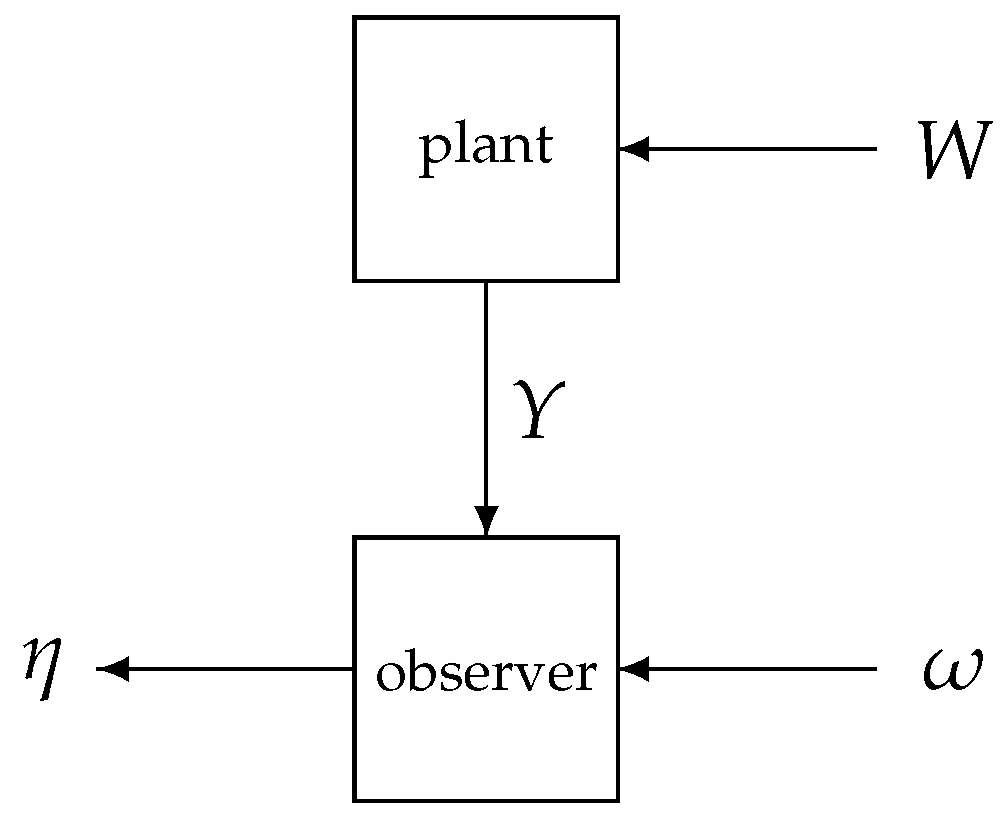
Suppose the quantum plant is cascaded in a measurement-free field-mediated fashion with another open quantum system, playing the role a coherent quantum observer, which is driven by the plant output Y and another quantum Wiener process $\omega$ of an even dimension $\mu$ on a different bosonic Fock space $\mathfrak{F}$; see Fig. Figure 1.

The observer is endowed with its own initial Hilbert space $\mathfrak{H}$, dynamic variables ${\xi }_1\left(t\right),\dots ,{\xi }_{\nu }\left(t\right)$ with a CCR matrix $\Lambda \in {\mathbb{A}}_{\nu }$ (so that $[\xi \left(t\right),\xi {\left(t\right)}^{\mathrm{T}}]=2i\Lambda$ for any $t⩾0$, similarly to (19)), and an $(m+\mu )$-dimensional output field $\eta \left(t\right)$:

$$\xi :={\left({\xi }_k\right)}_{1⩽k⩽\nu },\omega :={\left({\omega }_k\right)}_{1⩽k⩽\mu },\eta :={\left({\eta }_k\right)}_{1⩽k⩽m+\mu }.$$

(100)

Since the observer is driven by the plant output Y (together with the quantum noise $\omega$), the observer output $\eta$ acquires, over the course of time, quantum statistical correlations with the plant variables and can be used for estimating the latter in a mean square optimal fashion as specified below. To this end, we denote the observer Hamiltonian by $\Gamma$ and the vectors of operators of coupling of the observer with the plant output Y and with the quantum Wiener process $\omega$ by

$$\Phi :={\left({\Phi }_k\right)}_{1⩽k⩽m},\Psi :={\left({\Psi }_k\right)}_{1⩽k⩽\mu },$$

(101)

respectively. The Hamiltonian $\Gamma$ and the coupling operators ${\Phi }_1,\dots ,{\Phi }_m$, ${\Psi }_1,\dots ,{\Psi }_{\mu }$ are functions of the dynamic variables ${\xi }_1,\dots ,{\xi }_{\nu }$ of the observer and hence, commute with the plant variables and functions thereof, including H, L. The plant and observer form a composite quantum stochastic system, whose vector $\mathcal{X}$ of dynamic variables satisfies the CCRs

$$[\mathcal{X},{\mathcal{X}}^{\mathrm{T}}]=2i\Theta ,\Theta :=\left[\begin{array}{cc}\Theta & 0\\ 0& \Lambda \end{array}\right],\mathcal{X}:=\left[\begin{array}{c}X\\ \xi \end{array}\right]$$

(102)

and is driven by an augmented quantum Wiener process $\mathcal{W}$ with the following Ito table:

$$\mathrm{d}\mathcal{W}\mathrm{d}{\mathcal{W}}^{\mathrm{T}}=\Omega \mathrm{d}t,\Omega :=\left[\begin{array}{cc}\Omega & 0\\ 0& \mho \end{array}\right]=I_{m+\mu }+iJ,J:=I_{(m+\mu )/2}\otimes \mathbf{J},\mathcal{W}:=\left[\begin{array}{c}W\\ \omega \end{array}\right].$$

(103)

Here, ℧ is the Ito matrix of the quantum Wiener process $\omega$ of the observer, which is defined similarly to $\Omega$ from (1), (2) as

$$\mathrm{d}\omega \mathrm{d}{\omega }^{\mathrm{T}}=\mho \mathrm{d}t,\mho :=I_{\mu }+i{I}_{\mu /2}\otimes \mathbf{J}.$$

(104)

The quantum feedback network formalism [14] allows the Hamiltonian $\mathbf{H}$ of the plant-observer system and its vector $\mathbf{L}$ of operators of coupling with $\mathcal{W}$ to be computed as

$$\mathbf{H}=H+\Gamma +{\Phi }^{\mathrm{T}}JL,\mathbf{L}=\left[\begin{array}{c}L+\Phi \\ \Psi \end{array}\right].$$

(105)

Hence, the internal and output variables ${\xi }_1,\dots ,{\xi }_{\nu }$ and ${\eta }_1,\dots ,{\eta }_{m+\mu }$ of the observer in (100) are governed by the QSDEs

$$\begin{array}{cc}\hfill \mathrm{d}\xi & =\mathbf{G}\left(\xi \right)\mathrm{d}t-i[\xi ,{\mathbf{L}}^{\mathrm{T}}]\mathrm{d}\mathcal{W}=(i[\Gamma ,\xi ]+\Delta \left(\xi \right))\mathrm{d}t-i\left[\xi ,\left[\begin{array}{cc}{\Phi }^{\mathrm{T}}& {\Psi }^{\mathrm{T}}\end{array}\right]\right]\mathrm{d}\left[\begin{array}{c}Y\\ \omega \end{array}\right],\hfill \end{array}$$

(106)

$$\begin{array}{cc}\hfill \mathrm{d}\eta & =2J\mathbf{L}\mathrm{d}t+\mathrm{d}\mathcal{W}.\hfill \end{array}$$

(107)

Here,

$$\mathbf{G}\left(\zeta \right):=i[\mathbf{H},\zeta ]+\mathbf{D}\left(\zeta \right)$$

is the GKSL generator of the plant-observer system, and

$$\mathbf{D}\left(\zeta \right)=-[\zeta ,{\mathbf{L}}^{\mathrm{T}}]\Omega \mathbf{L}-\frac{1}{2}[{\mathbf{L}}^{\mathrm{T}}\Omega \mathbf{L},\zeta ]$$

is the corresponding decoherence superoperator, in accordance with (11), (103), (105). In (106), use is also made of the partial decoherence superoperator $\Delta$ which acts on the observer variables as

$$\Delta \left(\xi \right)=-[\xi ,{\Phi }^{\mathrm{T}}]\Omega \Phi -[\xi ,{\Psi }^{\mathrm{T}}]\mho \Psi -\frac{1}{2}[{\Phi }^{\mathrm{T}}\Omega \Phi +{\Psi }^{\mathrm{T}}\mho \Psi ,\xi ]$$

in view of (102)–(105). Now, consider a coherent quantum filtering (CQF) problem formulated as the minimisation of the mean square discrepancy

$$\mathcal{Z}:=\underset{t\to +\infty }{lim}\mathbf{E}Z\left(t\right)⟶min,Z:=\frac{1}{2}{(SX-T\mathbf{L})}^{\mathrm{T}}(SX-T\mathbf{L})$$

(108)

between r linear combinations of the plant variables of interest and the entries of the drift part $2J\mathbf{L}$ of the observer output $\eta$ in (107) as specified by given weighting matrices $S\in {\mathbb{R}}^{r\times n}$ and $T:=\left[\begin{array}{cc}{T}_1& T_2\end{array}\right]$, with $T_1\in {\mathbb{R}}^{r\times m}$, $T_2\in {\mathbb{R}}^{r\times \mu }$. The criterion process Z in (108) is similar to that in (83):

$$Z:=\frac{1}{2}\left[\begin{array}{cc}{X}^{\mathrm{T}}& {\mathbf{L}}^{\mathrm{T}}\end{array}\right]\Pi \left[\begin{array}{c}X\\ \mathbf{L}\end{array}\right],\Pi :=\left[\begin{array}{cc}{S}^{\mathrm{T}}S& -S^{\mathrm{T}}T\\ -T^{\mathrm{T}}S& T^{\mathrm{T}}T\end{array}\right],$$

(109)

with X being the only subvector of $\mathcal{X}$ from (102) which is present in (109). The minimization in (108) is over the observer Hamiltonian $\Gamma$ and the vector $\Phi$ of the observer-plant coupling operators in (101) as functions of the observer variables ${\xi }_1,\dots ,{\xi }_{\nu }$. This mean square optimal CQF problem extends [45] in that we do not restrict attention to linear observers even if the plant is an OQHO and $\Psi$ depends linearly on the observer variables $\xi$. Note that the Hamiltonian H of the plant and its coupling L to the input quantum noise W are fixed, and so also is the coupling $\Psi$ of the observer to the input quantum noise $\omega$; see Figure 1. If ${\Gamma }_0$, ${\Phi }_0$ are perturbed in the directions

$$K_0:={\Gamma }_0^{\prime },M_0:={\Phi }_0^{\prime },$$

(110)

consisting of self-adjoint operators representable as functions of the initial observer variables ${\xi }_1\left(0\right),\dots ,{\xi }_{\nu }\left(0\right)$, then the corresponding perturbations of the plant-observer Hamiltonian and coupling operators in (105) are

$${\mathbf{H}}_0^{\prime }=K_0+M_0^{\mathrm{T}}J{L}_0,{\mathbf{L}}_0^{\prime }=\left[\begin{array}{c}{M}_0\\ 0\end{array}\right].$$

(111)

By applying Theorem 2 and using (103), (110), (111), it follows that the corresponding transverse Hamiltonian Q for the plant-observer system satisfies the QSDE

$$\begin{array}{cc}\hfill \mathrm{d}Q& =\left(K+M^{\mathrm{T}}JL-\mathrm{Im}\left({\mathbf{L}}^{\mathrm{T}}\Omega \left[\begin{array}{c}M\\ 0\end{array}\right]\right)\right)\mathrm{d}t+\left[\begin{array}{cc}{M}^{\mathrm{T}}& 0\end{array}\right]\mathrm{d}\mathcal{W}\hfill \\ \hfill & =(K-\mathrm{Im}\left({(2L+\Phi )}^{\mathrm{T}}\Omega M\right))\mathrm{d}t+M^{\mathrm{T}}\mathrm{d}W,\hfill \end{array}$$

(112)

where use is also made of $\mathrm{Im}\left(L^{\mathrm{T}}\Omega M\right)=-M^{\mathrm{T}}JL$ (following from (1) and the commutativity $[L,M^{\mathrm{T}}]=0$). Then the Gateaux derivative ${\mathcal{Z}}^{\prime }$ of the cost functional in (108) is given by (80), where

$${\mathsf{j}}_t\left(Z_0^{\prime }\right)=\mathrm{Re}\left({(T\mathbf{L}-SX)}^{\mathrm{T}}{T}_{1}M\right)$$

in view of (109), (111) and similarly to (85). In accordance with (82), the expectation of the derivative process $\varphi :=i[Q,Z]$ satisfies the IDE

$${\left(\mathbf{E}\varphi \right)}^{{}^{\cdot }}=i\mathbf{E}[Q,\mathbf{G}\left(Z\right)]+\mathbf{E}\chi \left(Z\right),$$

where, in view of (112), the superoperator $\chi$ in (69) is given by

$$\chi \left(Z\right)=i[K-\mathrm{Im}\left({(2L+\Phi )}^{\mathrm{T}}\Omega M\right),Z]-2\mathrm{Re}\left([Z,{(L+\Phi )}^{\mathrm{T}}]\Omega M\right).$$

In particular, if both the plant and the unperturbed observer are OQHOs with Hurwitz dynamics matrices (while the perturbations in (110) are not necessarily linear-quadratic), then ${\mathcal{Z}}^{\prime }$ can be found (in a form similar to (93)) along the lines of Example 3 of Section 6 due to the criterion process Z in (108), (109) being a quadratic function of the plant and observer variables in $\mathcal{X}$ from (102).

The transverse Hamiltonian method, outlined above, was used in [47] for showing that, in the mean square optimal CQF problem for linear quantum plants, those observers, which are locally optimal in the class of linear quantum observers, cannot be improved locally (in the sense of the first-order optimality conditions (81)) by varying the Hamiltonian and coupling operators of the observer along linear combinations of the Weyl operators associated with the observer variables.

8. Concluding remarks

For a class of open quantum systems governed by Markovian Hudson-Parthasarathy QSDEs, we have introduced a transverse Hamiltonian and derivative processes associated with perturbations of the system Hamiltonian and system-field coupling operators. This provides a fully quantum tool for infinitesimal perturbation analysis of system operators and cost functionals which involve averaging over the invariant quantum state of the system. The proposed variational method can be used for the development of first-order necessary conditions of optimality in quantum control and filtering problems. We have illustrated these ideas for OQHOs with quadratic performance criteria and the mean square optimal CQF problem.

References

- Anderson, B.D.O.; Moore, J.B. Optimal Control: Linear Quadratic Methods; Prentice Hall: London, 1989. [Google Scholar]
- Belavkin, V.P. Quantum filtering of Markovian signals with quantum white noises. Radiotekhn. i Elektron. 1980, 25, 1445–1453. [Google Scholar]
- Belavkin, V.P. On the theory of controlling observable quantum systems. Autom. Remote Control 1983, 44, 178–188. [Google Scholar]
- Belavkin, V.P. Quantum stochastic calculus and quantum nonlinear filtering, J. Multivar. Anal. 1992, 42, 171–201. [Google Scholar] [CrossRef]
- Boukas, A. Stochastic control of operator-valued processes in boson Fock space. Russian J. Math. Phys. 1996, 4, 139–150. [Google Scholar]
- Breuer, H.-P.; Petruccione, F. The Theory of Open Quantum Systems; Clarendon Press: Oxford, 2006. [Google Scholar]
- Cushen, C.D.; Hudson, R.L. A quantum-mechanical central limit theorem. J. Appl. Prob. 1971, 8, 454–469. [Google Scholar] [CrossRef]
- Dong, D.; Petersen, I.R. Quantum control theory and applications: a survey. IET Contr. Theor. Appl. 2010, 4, 2651–2671. [Google Scholar] [CrossRef]
- Edwards, S.C.; Belavkin, V.P. Optimal quantum filtering and quantum feedback control. Available online: URL https://arxiv.org/abs/quant-ph/0506018 (arXiv:quant-ph/0506018v2, 1 August 2005).
- Folland, G.B. Harmonic Analysis in Phase Space; Princeton University Press: Princeton, 1989. [Google Scholar]
- Gardiner, C.W.; Zoller, P. Quantum Noise, 3rd Ed. ed; Springer: Berlin, 2004. [Google Scholar]
- Gorini, V.; Kossakowski, A.; Sudarshan, E.C.G. Completely positive dynamical semigroups of N-level systems. J. Math. Phys. 1976, 17, 821–825. [Google Scholar] [CrossRef]
- Gough, J.; Belavkin, V.P.; Smolyanov, O.G. Hamilton-Jacobi-Bellman equations for quantum optimal feedback control. J. Opt. B: Quant. Semiclass. Opt. 2005, 7, S237–S244. [Google Scholar] [CrossRef]
- Gough, J.; James, M.R. Quantum feedback networks: Hamiltonian formulation. Commun. Math. Phys. 2009, 287, 1109–1132. [Google Scholar] [CrossRef]
- Holevo, A.S. Quantum stochastic calculus. J. Math. Sci. 1991, 56, 2609–2624. [Google Scholar] [CrossRef]
- Holevo, A.S. Statistical Structure of Quantum Theory; Springer: Berlin, 2001. [Google Scholar]
- Horn, R.A.; Johnson, C.R. Matrix Analysis; Cambridge University Press: New York, 2007. [Google Scholar]
- Higham, N.J. Functions of Matrices; SIAM: Philadelphia, 2008. [Google Scholar]
- Hudson, R.L.; Parthasarathy, K.R. Quantum Ito’s formula and stochastic evolutions. Commun. Math. Phys. 1984, 93, 301–323. [Google Scholar] [CrossRef]
- Jacobs, K.; Knight, P.L. Linear quantum trajectories: applications to continuous projection measurements. Phys. Rev. A 1998, 57, 2301–2310. [Google Scholar] [CrossRef]
- Janson, S. Gaussian Hilbert Spaces; Cambridge University Press: Cambridge, 1997. [Google Scholar]
- James, M.R.; Nurdin, H.I.; Petersen, I.R. H∞ control of linear quantum stochastic systems. IEEE Trans. Automat. Contr. 2008, 53, 1787–1803. [Google Scholar] [CrossRef]
- Kallianpur, G. Stochastic Filtering Theory; Springer: New York, 1980. [Google Scholar]
- Karatzas, I.; Shreve, S.E. Brownian Motion and Stochastic Calculus, 2nd Ed. ed; Springer-Verlag: New York, 1991. [Google Scholar]
- Kwakernaak, H.; Sivan, R. Linear Optimal Control Systems; Wiley: New York, 1972. [Google Scholar]
- Landau, L.D.; Lifshitz, E.M. Statistical Physics, 3rd Ed. ed; Elsevier: Amsterdam, 1980. [Google Scholar]
- Lindblad, G. On the generators of quantum dynamical semigroups. Commun. Math. Phys. 1976, 48, 119–130. [Google Scholar] [CrossRef]
- Liptser, R.S.; Shiryayev, A.N. Statistics of Random Processes I: General Theory; Springer-Verlag: Berlin, 1977. [Google Scholar]
- Merzbacher, E. Quantum Mechanics, 3rd Ed. ed; Wiley: New York, 1998. [Google Scholar]
- Meyer, P.-A. Quantum Probability for Probabilists; Springer: Berlin, 1995. [Google Scholar]
- Miao, Z.; James, M.R. Quantum observer for linear quantum stochastic systems. In Proceedings of the 51st IEEE Conf. Decision Control, Maui, Hawaii, USA, 1680–1684., 10-13 December 2012. [Google Scholar]
- Nielsen, M.A.; Chuang, I.L. Quantum Computation and Quantum Information; Cambridge University Press: Cambridge, 2000. [Google Scholar]
- Nurdin, H.I.; James, M.R.; Petersen, I.R. Coherent quantum LQG control. Automatica 2009, 45, 1837–1846. [Google Scholar] [CrossRef]
- Nurdin, H.I.; Yamamoto, N. Linear Dynamical Quantum Systems; Springer: Netherlands, 2017. [Google Scholar]
- Parthasarathy, K.R. An Introduction to Quantum Stochastic Calculus; Birkhäuser: Basel, 1992. [Google Scholar]
- Parthasarathy, K.R. What is a Gaussian state? Commun. Stoch. Anal. 2010, 4, 143–160. [Google Scholar] [CrossRef]
- Parthasarathy, K.R.; Schmidt, K. Positive Definite Kernels, Continuous Tensor Products, and Central Limit Theorems of Probability Theory; Springer-Verlag: Berlin, 1972. [Google Scholar]
- Petersen, I.R. Quantum linear systems theory. Open Automat. Contr. Syst. J. 2017, 8, 67–93. [Google Scholar] [CrossRef]
- Sakurai, J.J. Modern Quantum Mechanics; Addison-Wesley: Reading, Mass, 1994. [Google Scholar]
- Shaiju, A.J.; Petersen, I.R. A frequency domain condition for the physical realizability of linear quantum systems. IEEE Trans. Automat. Contr. 2012, 57, 2033–2044. [Google Scholar] [CrossRef]
- Shiryaev, A.N. Probability, 2nd Ed. ed; Springer: New York, 1996. [Google Scholar]
- Sichani, A.K.; Vladimirov, I.G.; Petersen, I.R. A numerical approach to optimal coherent quantum LQG controller design using gradient descent. Automatica 2017, 85, 314–326. [Google Scholar] [CrossRef]
- Stroock, D.W. Partial Differential Equations for Probabilists; Cambridge University Press: Cambridge, 2008. [Google Scholar]
- Vladimirov, I.G.; Petersen, I.R. A quasi-separation principle and Newton-like scheme for coherent quantum LQG control. Syst. Contr. Lett. 2013, 62, 550–559. [Google Scholar] [CrossRef]
- Vladimirov, I.G.; Petersen, I.R. Coherent quantum filtering for physically realizable linear quantum plants. In Proceedings of the European Control Conference, Zurich, Switzerland, 2717–2723., 17-19 July 2013. [Google Scholar]
- Vladimirov, I.G. A quantum mechanical version of Price’s theorem for Gaussian states. In Proceedings of the 4th Australian Control Conference, Canberra, Australia, 118–123., 17-18 November 2014. [Google Scholar]
- Vladimirov, I.G. Weyl variations and local sufficiency of linear observers in the mean square optimal coherent quantum filtering problem. In Proceedings of the 5th Australian Control Conference, Gold Coast, Australia, 93–98., 5-6 November 2015. [Google Scholar]
- Vladimirov, I.G. A transverse Hamiltonian variational technique for open quantum stochastic systems and its application to coherent quantum control. In Proceedings of the 2015 IEEE Conference on Control Applications (CCA), Sydney, NSW, Australia, 29–34., 21-23 September 2015. [Google Scholar]
- Vladimirov, I.G. A phase-space formulation and Gaussian approximation of the filtering equations for nonlinear quantum stochastic systems. Contr. Theory Techn. 2017, 15, 177–192. [Google Scholar] [CrossRef]
- Walls, D.F.; Milburn, G.J. Quantum Optics, Springer, Berlin, 2008.
- Wiseman, H.M.; Milburn, G.J. Quantum Measurement and Control; Cambridge University Press: Cambridge, 2010. [Google Scholar]
- Yanagisawa, M.; Kimura, H. Transfer function approach to quantum control – part I: dynamics of quantum feedback systems, part II: control concepts and applications. IEEE Trans. Automat. Contr. 2003, 48, 2107–2120. [Google Scholar] [CrossRef]
- Yosida, K. Functional Analysis, 6th Ed. ed; Springer: Berlin, 1980. [Google Scholar]
- Zhang, G.; James, M.R. Direct and indirect couplings in coherent feedback control of linear quantum systems. IEEE Trans. Automat. Contr. 2011, 56, 1535–1550. [Google Scholar] [CrossRef]
- Zhang, G.; Dong, Z. Linear quantum systems: a tutorial. Annual Reviews in Control 2022, 54, 274–294. [Google Scholar] [CrossRef]
Figure 1.
The series connection of a quantum plant with a coherent quantum observer, mediated by the plant output field Y and affected by the environment through the input quantum Wiener processes W, . The observer design objective is that the drift part of its output has to approximate the plant variables of interest in a mean square optimal fashion.
Disclaimer/Publisher’s Note: The statements, opinions and data contained in all publications are solely those of the individual author(s) and contributor(s) and not of MDPI and/or the editor(s). MDPI and/or the editor(s) disclaim responsibility for any injury to people or property resulting from any ideas, methods, instructions or products referred to in the content. |
© 2023 by the author. Licensee MDPI, Basel, Switzerland. This article is an open access article distributed under the terms and conditions of the Creative Commons Attribution (CC BY) license (https://creativecommons.org/licenses/by/4.0/).
Copyright: This open access article is published under a Creative Commons CC BY 4.0 license, which permit the free download, distribution, and reuse, provided that the author and preprint are cited in any reuse.