Submitted:
14 April 2023
Posted:
17 April 2023
You are already at the latest version
Abstract
The article presents an analysis of monthly precipitation totals based on the GPCC database, and monthly mean temperatures (NOAA data) for 377 catchments distributed across the globe. The analysis included 110-year data sequences from 1901 to 2010 calculated from grid data with a spatial resolution of 0.5°x 0.5° longitude and latitude. Long-term sequences of precipitation and temperature were used to assess the polarization of climatic phenomena. The noticeable impact of polarization in the area of extreme changes in temperature and precipitation is related to anthropogenic factors such as greenhouse gas emissions, deforestation and pollution, which affect ecosystem functioning, biodiversity, water resources and economies. The paper demonstrates the existence of trends related to the polarization of temperature and precipitation phenomena. The measures of polarization used in science are discussed. A simple measure of polarization was proposed and applied to both long-term sequences of monthly precipitation totals and monthly mean temperature. Due to the nature of the proposed polarization measure, other characteristics of the precipitation and temperature sequences are also presented as background for the discussion of the polarization index. The paper presents, for a selection of several hundred catchments from around the world, analyses of the assessment of precipitation and temperature trends using non-parametric tests. The trend analyses use Mann -Kendall tests at the 5% significance level. A Pettitt test was used to determine the trend change point for precipitation and temperature data. The whole is supported by rich graphical analyses and the results are presented tabularly.
Keywords:
polarization of climatic phenomena
; GPCC data
; NOAA data
; monthly precipitation
; average temperature
; climate trends
; Mann Kendall test
; Pettitt test
1. Introduction
Analysis of historical observations of climate variables indicates anthropogenic climate change [1,2,3]. Numerous studies at various spatial scales have considered the impact of projected changes in the climate system on hydrology and water resources [1,3,4,5,6]. Freshwater availability is the second most responsive environmental variable to climate change after air temperaturę [1,7,8,9,10]. The timeliness of temporal and spatial characteristics of precipitation and temperature, despite the many papers that have been written and analyses performed [11,12,13,14,15,16,17,18] especially in recent decades is increasing due to the documentation of theses of the impact of human activities on regional climatic factors [19,20,21]. Computational capabilities and complex analyses performed on long series of measurements are attracting interest [8,22,23] also as a result of the search for justification of theses of polarization of extreme phenomena [1,24,25,26,27,28,29,30]. The renewed interest in climatic factors including precipitation and temperature [13,31,32] is also due to accumulations of flood damage and periods of hydrological drought [33]. The study of changes in the amount of precipitation and temperature variability [5,9,14,34,35,36] depending on the observed period show changes in statistical trends and allow us to assess the form of the directions of these changes occurring [32,37,38,39]. The results of the evaluation of precipitation trends and temperature trends provide an opportunity to indicate the moment of trend change and determine the form of this trend. Given the importance of the variability of climate factors on water resources, an important research element is the use of statistical techniques [4] , [40] that allow the detection of changes and trends [2,38] in such characteristics as data of monthly precipitation totals and average monthly temperature, among others.
The Intergovernmental Panel on Climate Change (IPCC) predicts that increased greenhouse gas emissions following the industrialization of the world, due to large-scale burning of fossil fuels, human interference and land use change, will increase global temperatures [3,10,41,42]. The Intergovernmental Panel on Climate Change [43] noted that natural forces and human activities contribute significantly to changing climate patterns, i.e., increasing land and ocean surface temperatures, changing spatial and temporal precipitation patterns, increasing the frequency of extreme events, sea level rise and intensifying El Niño [3,4,31,34]. An average increase in global temperature of 0.6°C from 1901 to 2001 indicates that the Earth has been warming over the past many decades [43]. Changes in trends of precipitation and temperature can be observed and evaluated on the basis of anomalous values. The change in trends of various climatic variables can be quantified through the use of global circulation models (GCMs) or, for example, through the use of statistical models that recognize the timing of the trend change and its magnitude [8] . Polarization of climatic phenomena has been demonstrated [35], who found increasing trends mainly in flood climaxes in German river basins, which was attributed to climate change. In addition, seasonal analyses showed that these changes were greater in winter than in summer. Climate variability has a significant impact on flow values, which are sensitive to both precipitation and temperature. Many other studies have documented that human and economic activities can play an important role in reducing flow values directly related to precipitation. Many researchers have investigated the existence of a change point in the observed time series. Rapid changes, both in mean and variance, can be related to both climate (e.g., shifts in climate regimes, and anthropogenic effects (e.g., construction of dams and reservoir systems, changes in land use/land cover and agricultural practices, relocation of measurement points) [44,45]. Statistical analyses must be interpreted in conjunction with observed physical [3,7,46], social and economic phenomena [3,14,19,47]. Precipitation and temperature are very important climatic parameters because their changes can affect living conditions. Therefore, predicting temporal trends of precipitation and temperature is very useful in social and urban planning [48].
The world's rivers carry 40% of precipitation as runoff from the land and 95% of sediment to the oceans, linking the atmosphere, hydrosphere and biosphere [49,50]. Precipitation and temperature are among the main factors, along with evaporation, affecting the polarization of runoff. In this work, long-term sequences of precipitation and temperature are analyzed, which is also directly related to evaporation [51]. The analyses performed provide a basis for determining directions for the creation of decision-making tools to control extreme drought and flood events, as well as for assessing and preventing ecological damage in threatened regions [52].
In assessing the polarization of climate phenomena, there are strong relationships between precipitation amounts and temperature [34,52,53]. An increase in global temperature can lead to an increase in water vapor in the atmosphere, which in turn can increase precipitation. In the case of lower temperatures, the opposite can occur, i.e. a decrease in precipitation. In extreme cases, such as prolonged droughts or floods, changes in temperature and precipitation can lead to catastrophic consequences, such as crop loss or property damage [1,45,54]. Proper monitoring of precipitation and temperature is crucial to understanding climate change and assessing the polarization of climate phenomena [55]. Long-term data series make it possible to identify trends in temperature and precipitation and to determine whether a particular location is experiencing polarization changes. In addition, analyzing the interrelationship between precipitation and temperature allows us to understand the magnitude of atmospheric phenomena, such as El Niño and La Niña cycles [56], which affect the global climate. An increase in temperature can affect the occurrence of intense precipitation, and a decrease in precipitation can lead to extreme heat waves [45]. It is also important to analyze precipitation amounts and temperature in the context of other climate phenomena, as interactions between these phenomena affect the ultimate effects of climate polarization [57]. Relationships between precipitation and temperature magnitudes are important for assessing the polarization of climate phenomena. Knowledge of these relationships is essential for understanding the impact of climate change on the environment, economy and society, as well as for taking action to reduce the negative effects of climate change.
2. Data accepted for analysis
The great interest in analyzing long precipitation sequences stems from the need to assess climate change and its impacts at all spatial scales. This demand has led to the initiation and support of many research and monitoring programs conducted by international organizations. In this context, the Global Precipitation Climatology Center (GPCC) was established on behalf of the World Meteorological Organization (WMO) in 1989. This institution is supported and operated by the Deutscher Wetterdienst (DWD, Germany's National Meteorological Service) as a German contribution to the World Climate Research Program (WCRP). The main objective of the GPCC is the global analysis of monthly precipitation on the Earth's surface based on "in situ" precipitation station data [31,58]. An equally important institution is NOAA (National Oceanic and Atmospheric Administration) the US government agency for the study of the atmosphere, oceans and climate. It conducts research and monitoring of climate change, including collecting, processing, analyzing, updating and making available long-term precipitation and temperature sequences [59,60].
The goal of the aforementioned institutions is to meet users' requirements for the accuracy of the data and analysis results made available, as well as the timeliness and availability of the product. Among the various types of GPCC and NOAA products, gridded sets of long-term precipitation and temperature data, among others, are made available [58,59]. These data are not made available in real time. This paper relies on grid data of monthly precipitation totals from the GPCC products made available and grid data of monthly mean temperatures from NOAA products. The data correspond to a spatial resolution of 0.5°x 0.5°, and are consistent in spatial and temporal extent. Products from both the GPCCC and NOAA are made available via the Internet.
NOAA (National Oceanic and Atmospheric Administration) and GPCC (Global Precipitation Climatology Center) are two institutions that provide the opportunity, based on the long-term data made available, to perform analysis and evaluation of the polarization of climatic phenomena, precipitation and temperatures. NOAA is engaged in research and monitoring of the atmosphere, oceans and climate around the world. NOAA collects data from various sources such as satellites, ocean buoys, aircraft and weather stations to assess the state of the climate and predict changes. The GPCC is involved in assessing precipitation around the world. GPCC uses a variety of data sources, such as weather stations, radar and satellites, to develop global precipitation maps. The two institutions use their knowledge and data to assess changes in climate phenomena, including precipitation and temperatures around the world, and predict how they will change in the future. They are also working with other climate institutions to increase understanding of the climate and to help make decisions about climate change.This paper examines global trends in monthly precipitation totals and monthly mean temperatures from the area of 377 river basins distributed over all continents. Assuming 509.9 106 square kilometers of land area, 12.76% of the land area is included in the analysis. Table 1 shows the areas covered by the analysis.
GPCC data, rainfall totals by month from 1901 to 2010, calculated from grid data with a spatial resolution of 0.5°x 0.5° longitude and latitude, were converted to catchment areas. In this way, a sequence of monthly precipitation was obtained, which became the subject of the analyses presented in this article. GIS interpolation mechanisms were used in the spatial analysis of data preparation. The calculated values of the sequences were subjected to a simple statistical analysis, determining the basic statistics: the minimum and maximum value, the mean, the standard deviation of the sample and the value of the coefficient of variation. The data were analyzed in monthly cross sections as well as calendar years. Analyses of monthly precipitation covered the years 1901 to 2010.
NOAA monthly mean temperature data, from 1901 to 2010, calculated from grid data with a spatial resolution of 0.5°x 0.5° longitude and latitude, were converted to catchment areas. In this way, sequences of monthly average temperatures were obtained, which became the subject of the analyses presented in this article. GIS interpolation mechanisms were used in the spatial analysis of data preparation. The calculated values of the sequences were subjected to a simple statistical analysis, determining the basic statistics: the minimum and maximum value, the mean, the standard deviation of the sample and the value of the coefficient of variation. The data were analyzed in monthly as well as calendar year cross sections. Analyses of temperature data covered the years 1901 to 2010.
4. Polarization of precipitation and temperature phenomena
The occurrence of temporal variability and extreme events in air temperature and precipitation is usually assessed by analyzing a set of indicators that define variability and extreme conditions [39]. The common understanding of an extreme event is based on the assumption that a "normal" condition exists. In the context of the common understanding of an extreme event, polarization can be interpreted as a change in the nature of the occurrence of extremes, with extreme events - droughts, floods, extreme temperatures and precipitation - becoming more frequent, and the "normal" state becoming less frequent. Polarization of extreme events can result from a variety of factors, including human activities and climate change, which can affect precipitation cycles, the intensity of extreme events and temperature conditions. In this way, polarization can be seen as a process in which climate characteristics change and extreme events become more frequent, while the "normal" state becomes increasingly unstable. Polarization can have serious consequences for the functioning of ecosystems, the economy, and people's quality of life.
Analysis of the polarization of precipitation and temperature is essential because of their key role in the global energy and water cycles and their impact on climate change. Accurate knowledge of precipitation and temperature is particularly important for assessing the amount of available fresh water and managing water resources, which is essential for reducing the risk of floods and droughts. In addition, there is a growing body of scientific evidence confirming that human activities are influencing climate change, contributing to shorter periods of high-intensity precipitation and longer periods of high temperature and low precipitation. The polarization of extreme phenomena, such as floods and droughts, is increasingly evident and can be attributed to the unevenness and intensity of human activities. Therefore, studying polarization factors related to monthly precipitation and average monthly temperatures is key to understanding climate change at the regional level and developing strategies to manage water resources and reduce flood and drought risks.
This article analyzes long-term sequences of precipitation and temperature to assess the polarization of climate phenomena. The term "polarization" in terms of precipitation or temperature is used in climate science to describe the process by which certain areas of the planet become more extreme in terms of temperature or precipitation. This can lead to significant changes in the local environment, including changes in the distribution of plant and animal species, changes in weather patterns and changes in sea level [61]. Long-term sequences of precipitation and temperature are an essential tool for studying polarization in climate. These sequences provide a detailed record of an area's climate over many years, allowing the identification of trends and patterns in the data. By analyzing these sequences, it is possible to identify areas where the climate is becoming more polarized and track changes over time. One of the key advantages of using long-term precipitation and temperature sequences is that they provide a high degree of accuracy and precision. The time series are created using advanced measurement techniques, such as data from satellites and weather stations, and are subject to rigorous quality control measures [27,58,62]. As a result, they provide a highly reliable record of climate data in a given area, enabling precise observations and measurements.
The impact of polarization can be observed in various areas of life on Earth: in ecosystems, economy, and infrastructure, in changes in the size and location of water resources. The impact of polarization on ecosystems in areas of extreme temperature and precipitation changes affects biodiversity and ecosystem functioning [61]. Polarization of climate factors can lead to changes in the distribution of plant and animal species [63,64], which can have negative consequences for entire ecosystems. The consequences of polarization for agriculture can affect crops and food production [17,36]. In some regions, climate polarization can lead to a decrease in the amount of available water resources, which in turn will affect agricultural production and the condition of industry. The consequences of polarization for infrastructure can affect roads, bridges, buildings, water and sewerage networks, and water management systems. In extreme cases, serious damage or destruction may occur. The variability and difficulties in predicting polarization - due to the complex and dynamic nature of climate [65], it is difficult to predict exactly what the consequences of polarization will be in a given region. In addition, climate variability means that some regions may experience polarization in different years, complicating the process of predicting and monitoring changes. The interaction between polarization and other climate phenomena can affect other climate phenomena such as hurricanes, tornadoes, or droughts. In this way, one phenomenon can strengthen or weaken others, complicating the process of understanding the scale of climate change. The impact of anthropogenic factors on the polarization of climate factors, among other things, can occur through the emission of greenhouse gases [17,42,52,57]. Anthropogenic climate change, or changes resulting from human activity, leave a lasting mark on physical and biological systems around the world. Such changes include glacier melting, decline in some animal populations, changes in bird migration, and premature flowering of plants [66]. Analyzing the relationship between human activity and polarization can help understand and mitigate the negative effects of climate change.
The polarization of climate phenomena refers to changes in the intensity and frequency of extreme weather events, such as droughts, floods, hurricanes, and hailstorms. NOAA and GPCC monitor these changes [58,67] to determine the factors that influence the polarization of climate phenomena, their effects, and how to reduce the negative consequences associated with these events. Assessing temperature variability is crucial for understanding climate change and its impact on ecosystems and humans. All of this information is essential for developing strategies and actions to manage changes, adapt, and minimize their negative effects. NOAA and GPCC are a key source of information for scientists, policymakers, and other stakeholders who make decisions about climate change.
It is predicted that global warming will lead to an increase in the frequency of extreme weather events [1]. Although there is no direct evidence linking the increased frequency of extreme events to climate change, the observed positive trend indicates an increased likelihood of droughts and flash floods. Furthermore, changes in land use such as urbanization, reduction of natural retention, and improper water management can strongly influence the number of extreme events. The need to adapt water management to factors influencing the formation of water resources and the generation of hazards requires a comprehensive study of the current state and forecasts regarding the number, intensity, and frequency of extreme events. Extreme events such as droughts and floods can be characterized by their severity, duration, intensity, time between occurrences, and other direct and indirect parameters. Such a complex multiparameter characterization of these extreme events prompts modelers to simplify the description of the phenomenon and focus on one dominant parameter that is significant for the task or to use multidimensional methods, commonly used for example in frequency analysis (FFA, DFA) and risk analysis (FRA, DRA) [9,11,35,57,68].
5. The concept of polarization measure
The concept of measuring climate polarization is based on measuring the degree of diversity and variability of climate elements in a particular area. This measure is used to determine the level of polarization of climate elements in a given region. Polarization refers to extreme values of a parameter such as temperature, precipitation, humidity, etc., occurring in a specific area. A high level of polarization indicates significant differences between maximum and minimum values, which can lead to increased risk of extreme weather events. The measure of polarization can be determined based on different climatic parameters such as temperature, precipitation, humidity, atmospheric pressure, etc. It can be calculated on different spatial and temporal scales, for example, for the entire country over the course of a year, for a specific region over the course of a month, or for individual meteorological stations over the course of a day. Depending on the research purpose and data availability, the measure of polarization can be determined for different combinations of parameters. It is worth noting that a high level of polarization does not necessarily mean unfavorable climatic conditions. For example, in some regions, there are significant differences in temperature between summer and winter, which can have a positive impact on seasonal tourism. However, in other cases, high polarization can lead to serious problems such as droughts, floods, or storms. Therefore, the measure of polarization can be useful in identifying areas that require special attention when planning actions related to climate change adaptation.
Different approaches are possible for constructing measures of polarization in climate phenomena, depending on the type and scale of the analyzed data. One of the basic methods is to use probabilistic techniques based on classical theories of one- or multi-dimensional random variables with distributions built using copula functions [48,69,70]. Other, simpler methods are based on statistical characteristics [4,10,40,71]. A simple concept is to construct indicators measuring the degree of extremity that a phenomenon can take, for example, by measuring the dispersion relative to the long-term average. An example of such an indicator is the coefficient of variation. Another way to create a polarization indicator is to define it as the degree of extremity compared to the mean value, relative to variability measured by the dispersion measure [12,72,73]. Such indicators can be based on classical measures, such as variance, standard deviation, mean deviation, coefficient of variation, or on positional measures, such as range, quartile deviation, coefficient of variation [71].
Another method of constructing indicators is based on the idea of inequality [74,75], which can also be a measure of polarization. One such indicator is kurtosis, which is influenced by the intensity of extreme values and measures what happens in the "tails" of the distribution. Other types of indicators have their origins in economics and econometrics. An example is the Gini coefficient [73,76,77,78,79], which is constructed using the Lorenz curve, which describes the degree of concentration of a one-dimensional random variable with non-negative values [77]. The Gini coefficient ranges from a minimum value of zero when all values are equal, to a theoretical maximum of one in an infinite population where all but one element has a value of zero. In the context of climate change, the Gini coefficient can be used to measure inequality in exposure to climate change impacts such as droughts, floods, or sea level rise [57]. Higher Gini coefficient values indicate greater inequality in the occurrence of these phenomena.
Further methods of building indicators are based on the idea of unevenness [74,75], which can also be a measure of polarization. One such indicator is kurtosis, which is influenced by the intensity of extreme values, so it measures what is happening in the "tails" of the distribution. Other types of indicators are measures that have their genesis in economics and econometrics. An example is the Gini index [73,76,77,78,79] built using the Lorentz curve, which describes the degree of concentration of a one-dimensional distribution of a random variable with non-negative values [77]. The Gini index ranges from a minimum value of zero, when all values are equal, to a theoretical maximum of one in an infinite population in which every element except one has a magnitude of zero. In the context of climate change, the Gini index can be used to measure inequality in exposure to the effects of climate change, such as droughts, floods or sea level rise [57]. Higher values of the Gini index indicate greater inequality in the occurrence of these phenomena. Several other examples of measures can be cited, such as:
- The concentration ratio [80], which determines the degree of concentration of values at one end of the distribution, similar to the Gini coefficient. However, it should be noted that the Gini coefficient may be less useful in analyzing asymmetric distributions, which means that other indicators such as the concentration ratio or Lorenz curve should be considered in such cases.
- The GMD (Gini Mean Difference) index [81] is an inequality measure used in statistical and econometric analysis to measure polarization or inequality in a sample distribution. Unlike the Gini coefficient, which measures unevenness, the GMD index allows for the analysis of unevenness in the distribution of any variable, such as income, age, weight, height, precipitation, or temperature. The GMD index ranges from zero to one, where zero indicates complete evenness in the distribution, and one indicates concentration of all values in one class. The higher the GMD index value, the greater the unevenness in the variable distribution.
- Lorenz indicator [74,77] - is an inequality indicator in a distribution, which is based on the Lorenz curve. It is often used to measure income inequality but can also be used to measure inequality in other quantitative variables, including climate change studies. Higher values of the Lorenz curve indicate greater inequality in the occurrence of climate change effects such as droughts, floods, or sea level rise, meaning that some regions or social groups are more vulnerable to the effects of climate change than others.
- Atkinson index [73] - is a measure of inequality in the distribution of quantitative variables, which is based on the idea of absolute deviations. It takes into account the differences between groups of values in the distribution, similar to the Gini index, but focuses more on average values than extreme values.
- Range - values calculated as max-min usually refer to the difference between the maximum and minimum values of a given variable in a given period of time. In the case of assessing the polarization of precipitation and temperature, max-min can be used as a measure of the amplitude of these variables in a given period.
In this study, two measures are adopted to evaluate the phenomenon of polarization, the first is built based on static statistics, the second is based on calculated trends.
The first measure is defined as follows:
- the amplitude of changes, range, the difference between the maximum and minimum value of a variable, is a measure characterizing the empirical range of variability of the analyzed feature, - standard deviation.
values can be useful in identifying extreme climate conditions, such as periods of drought or heat waves, as well as periods of intense precipitation or extremely low temperatures. However, max-min as a single measure may be limited in its usefulness because it does not take into account other factors such as the length and intensity of the period, as well as other variables that affect weather conditions. Since it ignores all data except for two extreme values, it does not provide information about the diversity of individual feature values in the population. Therefore, along with max-min values, other measures such as mean values, standard deviations, or cumulative indices are typically used to obtain a more comprehensive and diverse view of climate variability. For example, max-min values can be calculated for individual months, seasons, or years, and then compared with mean values, standard deviations, or other measures to better understand climate variability over time and space.
The adopted measure, which is the ratio of the max-min values to the standard deviation , can be used as a measure to evaluate the polarization of precipitation and temperature. The values refer to the amplitude of changes of a given variable over a period of time, while the standard deviation σ refers to the degree of variability of these values around their mean. By applying this measure, we can see how large the amplitude of changes is in relation to the variability around the mean. Values of this measure greater than 1 suggest that the amplitude of changes is greater than the variability around the mean. If the variability is relatively low compared to the amplitude, it may indicate the occurrence of periods of extreme climatic conditions, such as periods of drought or heatwaves, as well as periods of intense rainfall or extremely low temperatures. However, the use of a single measure may be limited because it does not take into account other factors affecting climate variability. Therefore, it is worth using it together with other measures showing the character of climate variability. Note that the values of this measure for precipitation and temperature will always take a non-negative value.
The second form of adopted measures can be dynamic indicators showing the variability of the indicator over a longer period of time. The simplest indicators are based on the idea of a trend coefficient. The trend is a long-term feature, the general direction of changes over time in the value of a variable. The trend can indicate an increase, decrease, or stabilization of the variable over time. In time series analysis, the trend is one of the basic elements that help to forecast future values of the variable. The trend can be analyzed at different time scales, from short-term cycles to long-term trends [2]. Trend analysis is applied in many fields, such as economics, finance, meteorology, earth sciences, medicine, sociology, and marketing. In scientific research, trend analysis is often used to study changes in long-term time series, such as climate change, demographic changes, or evolution of species.
The second measure is defined as:
where is the trend of the amplitude of changes, range or difference between the maximum and minimum value of the variable - it is a measure characterizing the empirical range of variability of the studied feature, and is the standard deviation.
The above measure can be interpreted as the ratio of the trend in variability of the amplitude to the trend in variability of the standard deviation. The trend in variability of the amplitude refers to the direction and speed of changes in the maximum and minimum values of a given variable over time, while the trend in variability of the standard deviation refers to the direction and speed of changes in the variability of the values of a given variable around their mean over time. Values of this measure greater than 1 suggest that the trend in the increase of amplitude changes is stronger than the trend in the increase of variability around the mean. This means that changes in the maximum and minimum values of a given variable are increasing faster than the variability around their mean, which may indicate the occurrence of extreme weather conditions. In the proposed measure, the trend of the ratio of the indicators was not calculated, but the trend of the numerator and denominator was separately maintained. Both measures are used to assess trends in data, but they differ in how they relate to data variability.
The measure evaluates the trend magnitude by the variability of the data - the amplitude normalized by the standard deviation. changes are normalized by the standard deviation, which means that high changes in one direction can be balanced by changes in the opposite direction.
On the other hand, the measure uses two indicators of data variability: the trend of the amplitude and the trend of the standard deviation. The use of the amplitude in this formula means that extreme values of the data are emphasized more than their overall variability. Therefore, if we are more interested in extreme values in the data, the adopted measure may be a better choice. However, if we want to obtain a more balanced assessment of the trend, taking into account the overall variability of the data, the measure may be more appropriate. It should be noted that the values of this measure for precipitation and temperature can be negative and positive. In the case of negative values, this means that the trends of polarization factors (amplitude and variability) will be opposite, in the case of a positive value, the trends of polarization factors will be consistent.
6. Detecting a change point in the trend
Various methods can be applied to determine change points in a time series [83], [8,84,85,86]. In this analysis, the non-parametric Pettitt change point test [87] was used to detect the occurrence of changes. The Pettitt test is a non-parametric test for detecting sudden changes in a time sequence. It is used to detect the turning point where a sudden change, known as a "jump," occurs in the time series. The Pettitt test involves comparing the sum of ranks of two subsets of data, which are divided by a threshold value, to determine whether there is a statistically significant change in the time sequence. This test can be applied to analyze data with any distribution, and the test result is not dependent on the assumption of normality of the data. The result of the Pettitt test is a test statistic value, which is compared with the critical value for the level of significance to determine whether the null hypothesis of no sudden changes in the time sequence can be rejected.
The Pettitt test has been widely used to detect changes in observed climatic and hydrological time series [8,16,88,89]. The Pettitt test is also applicable to investigate an unknown change point by considering a sequence of random variables (X_1,X_2,...,X_T), which have a change point at τ. As a result, (X_1,X_2,...,X_τ) has a common distribution F_1 (·), but (X_(τ+1),X_(τ+2),...,X_T) has the same distribution as F_2 (·), where F_1 (·)≠F_2 (·). The null hypothesis H_0: no change (or τ=T); is tested against the alternative hypothesis H_1: change (or 1≤ τ <T); using the non-parametric statistic K_T = max|U_(t,T) |=max (K_(T+) ,K_(T-)) where:
The Pettitt test has been widely used to detect changes in observed climatic and hydrological time series [8,16,88,89]. The Pettitt test is also applicable to investigate an unknown change point by considering a sequence of random variables , which have a change point at . As a result has a common distribution , but has the same distribution as , where .The null hypothesis : no change (but ); is tested against the alternative hypothesis : change (lub ); using the non-parametric statistic where:
for the downward shift and or the upward shift [86]. The confidence level associated with lub is approximately determined by:
When is smaller than the specified confidence level (for example, in this study, 0.95 was adopted), the null hypothesis is rejected. The approximate probability of significance for the change point is defined as:
It is obvious that in the case of a significant change point, the series is segmented at the change point into two sub-time series.
The main aim of this study is to investigate the existence of change points in the time series of monthly sum precipitation and monthly average temperature characteristics. For time series showing a significant change point, the trend test will be applied to partial series, and if the change point is not significant, the trend test will be applied to the entire time series [8].
7. Trend test
To examine the trend in a given time series, the Mann-Kendall test can be applied. Originally, this test was used by Mann [90], and later Kendall in 1975 derived the distribution of the test statistic [86]. This test is independent of the type of distribution and we do not need to assume any specific form of the data distribution function [91]. This test was widely recommended by the World Meteorological Organization for public applications, and has been used in many scientific studies to assess trends in water resource data [2,8,86]. Therefore, the Mann-Kendall (MK) test has been recognized as an excellent tool for trend detection by other scholars in similar applications. It should also be noted that the MK test considers only the relative values of all elements in the series . for analysis. The test statistic for the MK test is given by:
where are the consecutive values of the data, and n is the number of elements in the data. Under the null hypothesis of no trend, and assuming that the data are independent and identically distributed with a zero mean and a variance denoted by , which is calculated as ( - the repeated values in the analyzed sequence):
To test hypotheses, the standard normal distribution, denoted as the test statistic , is used, which is defined as follows for the trend test::
In the two-sided test for trend, the null hypothesis is represented as: : there is no trend in the dataset, which will be rejected if the calculated statistic is greater than the critical value of this statistic obtained from the standard normal distribution table corresponding to the previously established level of significance. A positive value of indicates an increasing trend, and a negative value indicates a decreasing trend.
The magnitude of the trend is estimated using a non-parametric slope estimator based on the median, proposed by Sen [92] and extended by Hirsch [93]. The slope estimator is given by:
Where , and is treated as the median of all possible pairs of combinations for the entire dataset.
9. Results and Discussion
In the present study, the following properties of long-term sequences of monthly precipitation totals and monthly mean temperatures were investigated for 377 catchments from the area of 6 WMO regions. The scope of research and calculations included:
- the values of long-term sequences of 110 years in monthly cross sections were determined,
- statistics were calculated: average values for each calendar month, minimum value, maximum value, mean value, standard deviation (Table 2),
Table 1 shows the coverage of the continents with the areas of the analyzed catchments. A total of 12.76% of the land area out of 509.9 million square kilometers of land area was included in the analysis.
Statistical characteristics of monthly precipitation totals are presented in Table 2. It sequentially contains the following information: sequence number, GRDC code of the catchment, WMO (World Meteorological Organization) region code, river name, country code, catchment area [km2], then 12 columns of average monthly totals calculated for calendar months [mm], successively minimum value [mm], maximum value [mm] and standard deviation [mm].
The results of the analyses of trends and possible change points for the sequences of monthly precipitation totals are shown in Table 3. The following are included sequentially: sequence number, GRDC code of the catchment, WMO region code, river name, country code, measure, trend using TKM at 5% significance level for STD, trend using TKM at 5% significance level for RANGE, measure. , the year of the STD trend change, the year of the RANGE trend change, the significance probabilities for the STD and RANGE trend change point, the significance probabilities of the new STD and RANGE trend, the values of the new trends from the change point for STD and RANGE, and the value of the post-trend change polarization measure. Assuming a significance level of 5% only for the LAGARFLJOT river catchment located in Iceland, the change point of the trend in both RANGE and STD was shown, followed by the parameters of the new trend. The RANGE trend, changed not only the value but also the direction, from negative to positive, from a value of -0.136 changed to a value of 0.310 in 1953 and the STD trend from a value of -0.533 changed to a value of 0.889 also in 1953.
Based on the analysis of the data of monthly precipitation totals in the analyzed catchments, it should be noted that for 93/377 catchments, i.e. in 25% of the analyzed catchments, the trends of polarization factors (RANGE and STD) in the area of monthly precipitation totals were proved at the significance level of 5%. Analyzing the values (Table 3 and background of factors Table 2) of polarization factor trends sequentially in the 10 largest catchments with an area from 244000 - 2900000 km2, showed (/ c_v): NILE: 4.26/0.71, YENISEI: 4.25/0.64, YANGTZE RIVER: 5.28/ 0.66, GANGES: 3.81/1.24, HUANG HE: 6.11/1.01, BRAHMAPUTRA: 5.42/0.94, AMU DARYA: 5.10/0.83, EUPHRATES: 5.93/0.84, SENEGAL: 4.95/1.34, and URUGUAY: 7.15/1.34. The highest value of this assumed polarization index, among the 93 catchments, was obtained at 12.78 for the COPPER RIVER river catchment, the lowest at 3.81 for the GANGES river catchment.
Statistical characteristics of average monthly temperatures are presented in Table 4. It successively contains the following information: sequence number, GRDC code of the catchment, WMO (World Meteorological Organization) region code, river name, country code, catchment area [km2], then 12 columns of average monthly temperatures calculated for calendar months [°C], successively minimum value [°C], maximum value [°C] and standard deviation [°C].
The results of the trend anaAnalyzing the value (Table 3) of the trends of polarization factors (trend(RANGE) and trend(STD)) were shown at a significance level of 5%. The following values were obtained from the next 10 largest catchments ranging from 244000 - 2900000 km2, such as NILE: 2.28, YENISEI: 3.66, YANGTZE RIVER: 4.69, GANGES: 3.20, HUANG HE: 4.02, BRAHMAPUTRA: 5.17, AMU DARYA: 3.31, EUPHRATES: 3.81, SENEGAL: 3.00, and URUGUAY: 3.55. The highest value of this assumed polarization index, among 93 catchments, was obtained at 5.17 for the BRAHMAPUTRA river catchment, the lowest at 2.28 for the NILE river catchment.lyses and possible change points of the sequences of monthly average temperatures are shown in Table 5. The following are included sequentially: sequence number, GRDC code of the catchment, WMO region code, river name, country code, measure, trend using TKM at 5% significance level for STD, trend using TKM at 5% significance level for RANGE, measure. , the year of the STD trend change, the year of the RANGE trend change, the significance probabilities for the STD and RANGE trend change point, the significance probabilities of the new STD and RANGE trend, the values of the new trends from the change point for STD and RANGE, and the value of the post-trend change polarization measure.
Based on the analysis of the data of monthly average temperatures in the analyzed catchments, it should be noted that for 46/377 catchments, i.e., in 12.2% of the analyzed catchments, trends of polarization factors in the area of temperatures at the significance level of 5% have been proven. Analyzing the values (Table 5 and background of factors Table 4) trends of polarization factors (/ c_v) sequentially in the 10 largest catchments with an area of 190000 - 1730000 km2, such as, it is shown: AMUR: 3.42/-10.07, ORINOCO: 6.10/0.04, GANGES: 3.74/0.25, INDUS: 3.34/0.47, BRAHMAPUTRA: 3.39/0.63, SAO FRANCISCO: 5.24/0.07, VOLTA: 4.67/0.06, RIO PARNAIBA: 5.65/0.04, GODAVARI: 4.29/0.15, URAL: 3.87/3.87. The highest value of this assumed polarization index, among the 93 catchments, was obtained at 6.97 for the ESMERALDAS River catchment, the lowest at 6.10 for the ORINOCO River catchment.
Analyzing the value (Table 5) of the trends of the polarization factors for the next 10 largest catchments ranging from 190000 - 1730000 km2, showed: AMUR: 3.42, ORINOCO: 6.10, GANGES: 3.74, INDUS: 3.34, BRAHMAPUTRA: 3.39, SAO FRANCISCO: 5.24, VOLTA: 4.67, RIO PARNAIBA: 5.65, GODAVARI: 4.29, URAL: 3.87. The highest value of this assumed polarization index, among the 93 catchments, was obtained at 6.97 for the ESMERALDAS River catchment, the lowest at 6.10 for the ORINOCO River catchment.
Figure 1, shows the spatial location of the analyzed catchments in which significant polarization trends for monthly precipitation totals from 1901 to 2010 were recognized at the 5% significance level. The largest polarization values of 4 to 5.17 were recognized in catchments located in Asia in China- YANGTZE, India- BRAHMAPUTRA and Russia- YENISEI, Mid-West Africa- NIGER and in the Middle East: Iraq, TIGER river catchment.
Figure 2, shows the spatial location of the analyzed catchments in which significant trend change points in the polarity factors of monthly precipitation from 1901 to 2010 were recognized at the 5% significance level. Headline years of trend change were recognized from 1950 to 1980 in catchments located in the Asian area of China - YANGTZE, India - BRAHMAPUTRA and Russia - YENISEI, Midwest Africa- NIGER and the Middle East: Iraq, TIGER River catchment.
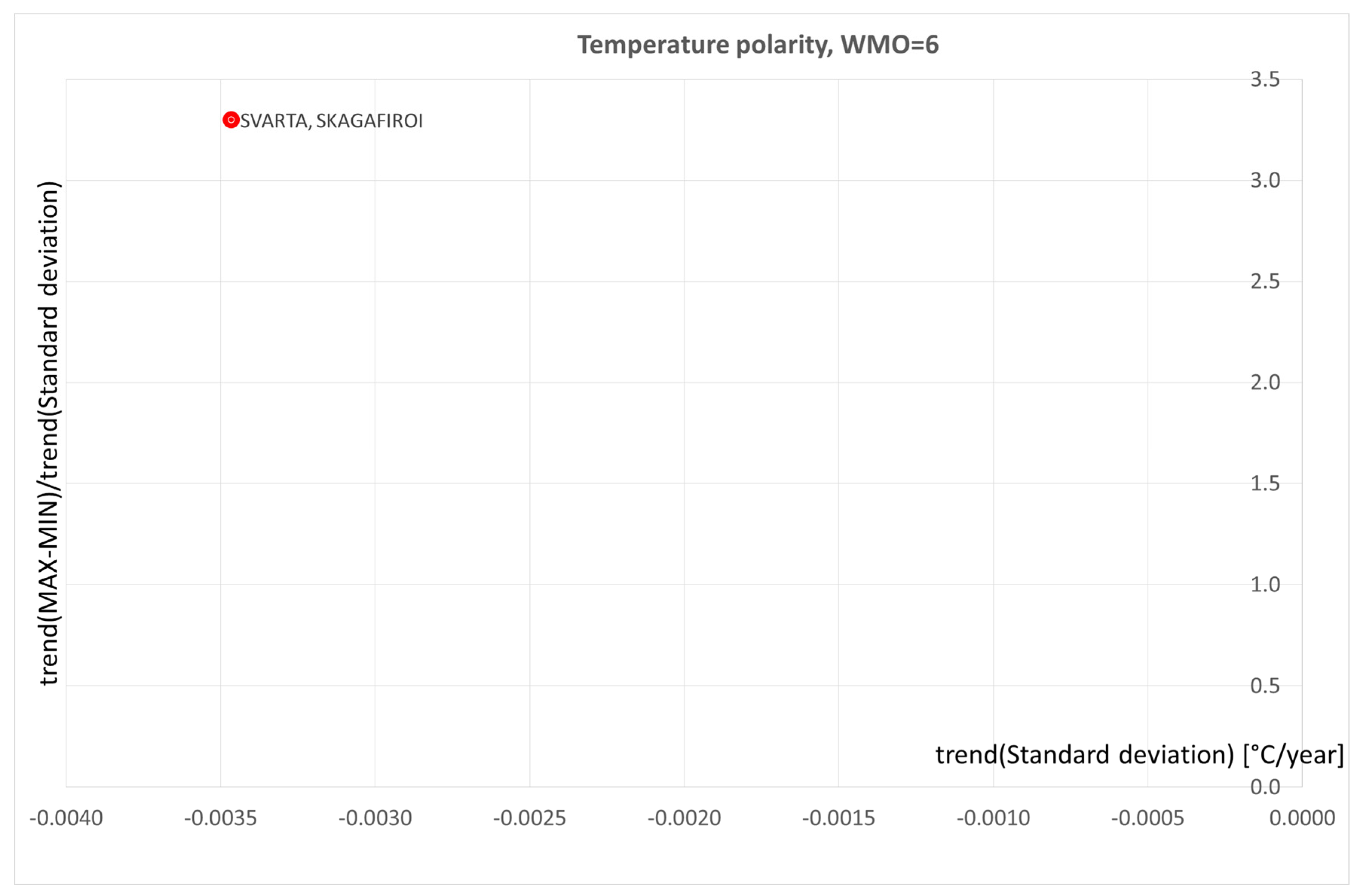
Figure 3, Figure 4, Figure 5, Figure 6, Figure 7, Figure 8 and Figure 9 and Figure 11, Figure 12, Figure 13, Figure 14, Figure 15 and Figure 16 show the results of the trend analyses paired with the trend(STD) value. This arrangement makes it possible to classify the analyzed catchments into four areas (quadrants) of the trend(STD)- arrangement showing the locations of catchments with the highest polarization indices of phenomena in both precipitation and temperature areas. Quadrant I is the area indicating an increase in the trend in amplitude and the trend in standard deviation (variability), quadrant II is the area with a negative trend in amplitude and a positive trend in variability, quadrant III is the area of catchment locations with a positive trend in amplitude and a negative trend in variability. Quadrant IV gathers catchments in which both trends are negative.
Figure 3, shows the polarity of in catchments on the continent of Africa. The location in quadrant IV indicates decreasing trends in the polarization factors in all the catchments indicated. Figure 4, shows the polarization of in the catchments of the continent of Asia. The largest values are in the BRAHMAPUTRA catchment. For this catchment, the trends of polarization factors are decreasing. In the case of the KARUN River catchment located in the 1st quadrant, both the trend of amplitude and variability are positive - the phenomena are increasing. Figure 5, shows the polarity of in the catchments of the South American continent. The largest values are in the RIO PARU DE ESTE catchment. For this catchment, the trends of polarization factors are decreasing. In the VINCES River catchment located in the 1st quadrant, both trends are increasing. Figure 6, shows the polarization of in the catchments of the North American continent. The largest values are in the SAVANNAH catchment, but both trends are decreasing. In the SAINT JOHN River catchment, on the other hand, both trends are increasing. Figure 7, shows the polarity of in the catchments of the continent of Australia and Oceania. The largest values are in the KINABATANGGAN catchment. For this catchment, the trends are decreasing. In the DE GREY River catchment, both trends are increasing. Figure 8, shows the polarity of in the catchments of continental Europe. The largest values are in the KIZILIRMAK catchment in Turkey. For this catchment, the trends are decreasing. In the KOKEMAENJOKI river catchment, both trends are increasing.
Figure 9, shows the spatial location of the analyzed catchments in which significant polarization trends were recognized at the 5% significance level for monthly average temperatures. from the period 1901 to 2010. The largest polarization values of more than 6.0 were recognized in the catchment located in the area of central West Africa- NIGER. Figure 10, shows the spatial location of the analyzed catchments in which significant trend change points in the polarization factors of monthly average temperatures from 1901 to 2010 were recognized at a significance level of 5%. Headline years of trend change were recognized in the period from 1940 to 1980 in catchments located in East Asia, India , central western Africa, central eastern South America and central North America.
Figure 9.
Watersheds in which significant polarization trends were identified for monthly mean temperatures during the period from 1901 to 2010 at a significance level of 5%.
Figure 9.
Watersheds in which significant polarization trends were identified for monthly mean temperatures during the period from 1901 to 2010 at a significance level of 5%.
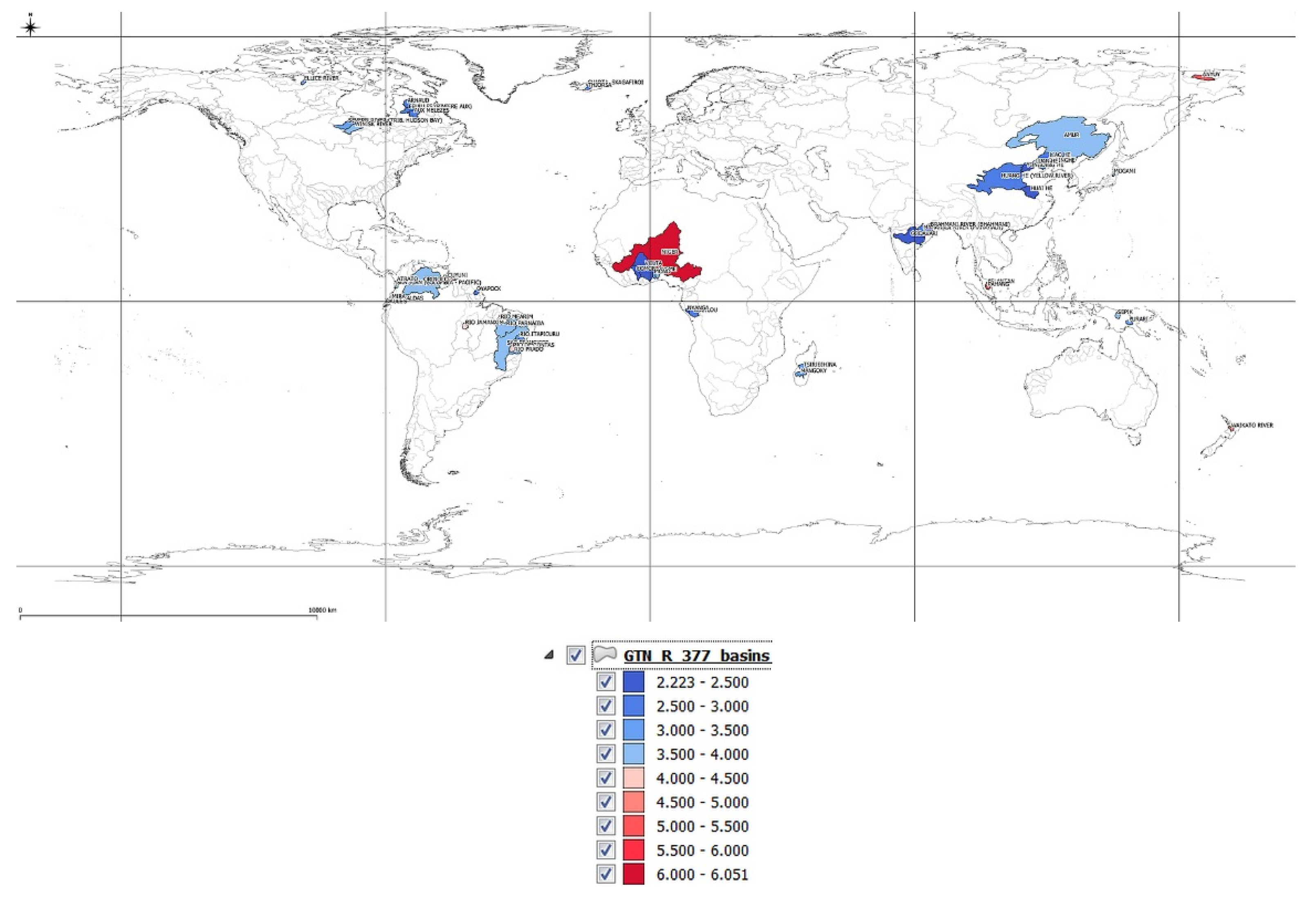
Figure 10.
Watersheds in which change points in the trend of factors related to temperature polarization for monthly mean temperatures during the period from 1901 to 2010 were identified at a significance level of 5%.
Figure 10.
Watersheds in which change points in the trend of factors related to temperature polarization for monthly mean temperatures during the period from 1901 to 2010 were identified at a significance level of 5%.
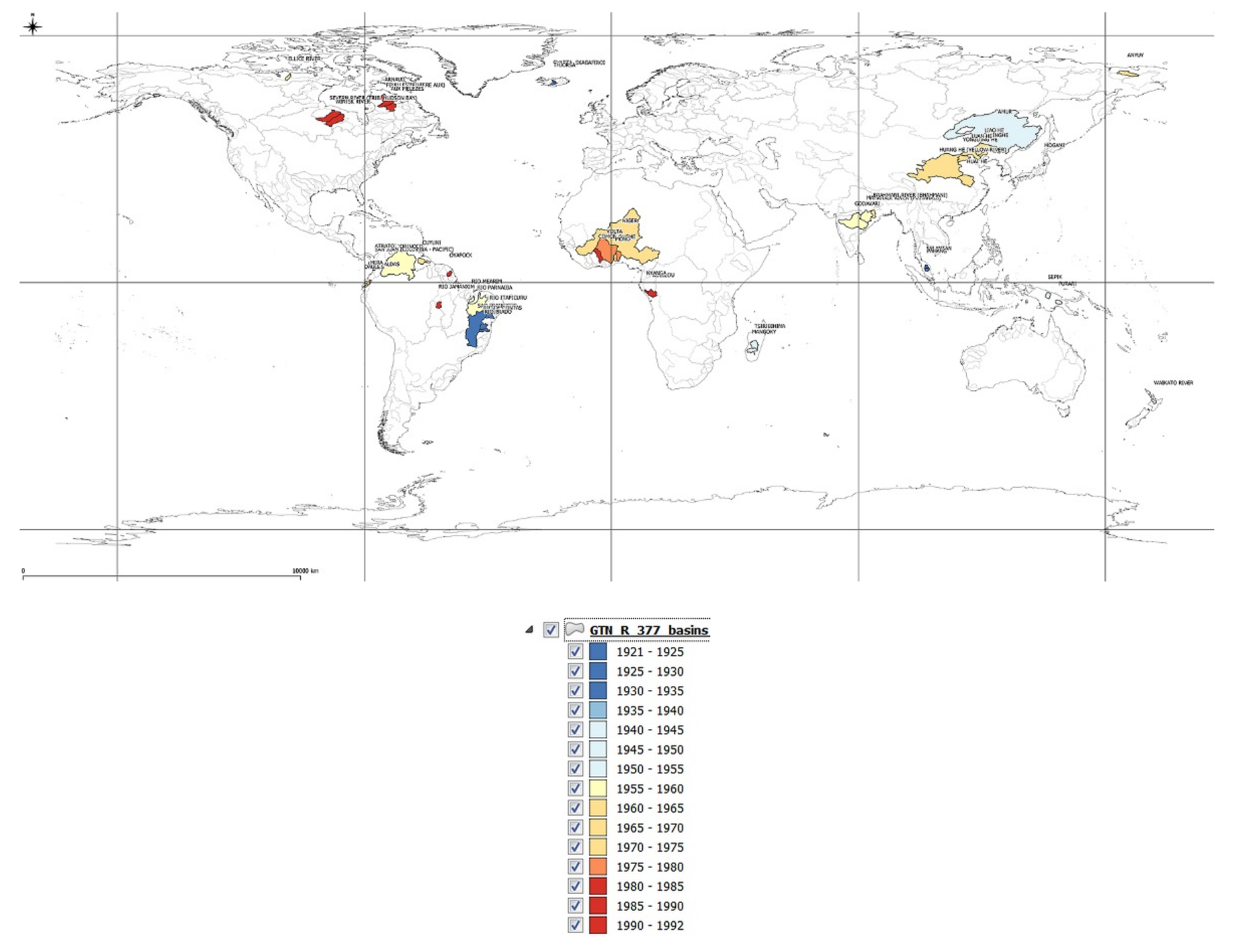
Figure 11, shows the polarization of in the area of average monthly temperatures in the catchments of the African continent. The largest values are in the MANGOKY and KOUILOU catchments with both trends decreasing.In the PRA and VOLTA river left, both trends are increasing. Figure 12, shows the polarity of in the area of average monthly temperatures in the catchments of the Asian continent. All catchments are in the area of negative trends of temperature polarization factors. The highest value is found in the AMUR catchment. Figure 13, shows the polarization in the area of average monthly temperatures in the catchments of the South American continent. The VINCES, ESMERALDAS and MIRA catchments located in quadrant IV are highlighted, i.e. both trends are decreasing. In quadrant I, the highest value of the index is found in the CUYUNI River catchment. Figure 14, shows the polarity of in the area of average monthly temperatures in the catchments of the North American continent. The catchment of the SAN PEDRO River shows increasing trends in the polarization factors. In the other catchments, both decreasing. Figure 15, shows the polarization of in the area of average monthly temperatures in the catchments of the continent of Australia and Oceania. The WAIKATO River catchment showed increasing trends in polarization factors. In the PURARI and DE GREY catchments, both show decreasing trends. Figure 16, shows polarization in the area of average monthly temperatures in the catchments of the European continent. The SVARTA river catchment showed decreasing trends of polarization factors.
Figure 11.
Watersheds in the region for which WMO_REG=1, in which significant polarization trends were identified for monthly mean temperatures during the period from 1901 to 2010 at a significance level of 5%.
Figure 11.
Watersheds in the region for which WMO_REG=1, in which significant polarization trends were identified for monthly mean temperatures during the period from 1901 to 2010 at a significance level of 5%.
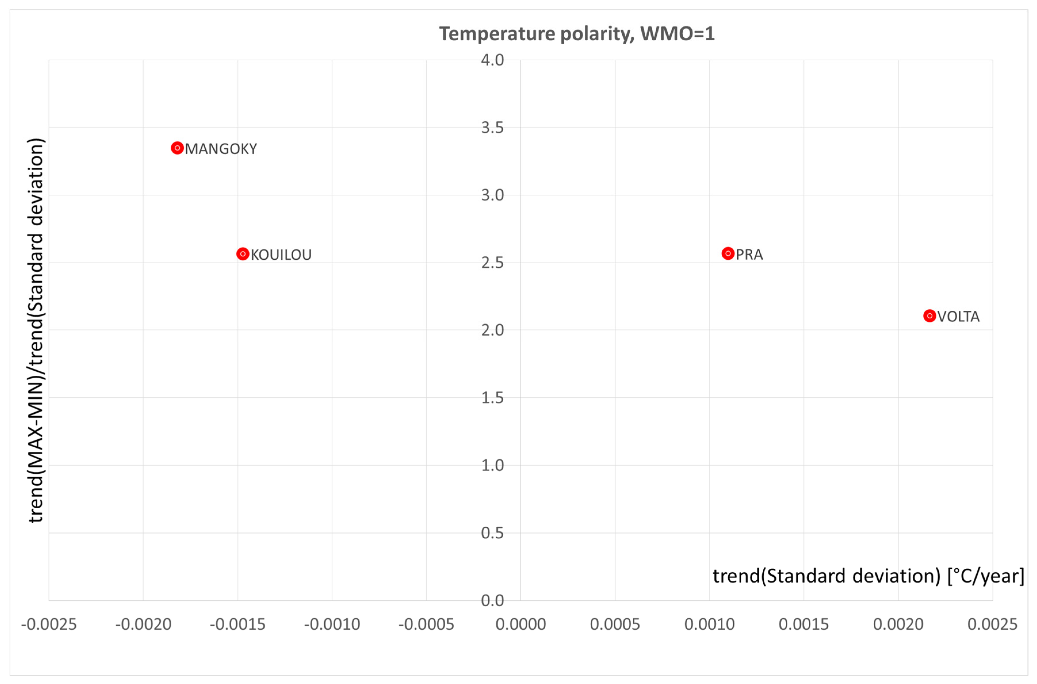
Figure 12.
Watersheds in the region for which WMO_REG=2, in which significant polarization trends were identified for monthly mean temperatures during the period from 1901 to 2010 at a significance level of 5%.
Figure 12.
Watersheds in the region for which WMO_REG=2, in which significant polarization trends were identified for monthly mean temperatures during the period from 1901 to 2010 at a significance level of 5%.
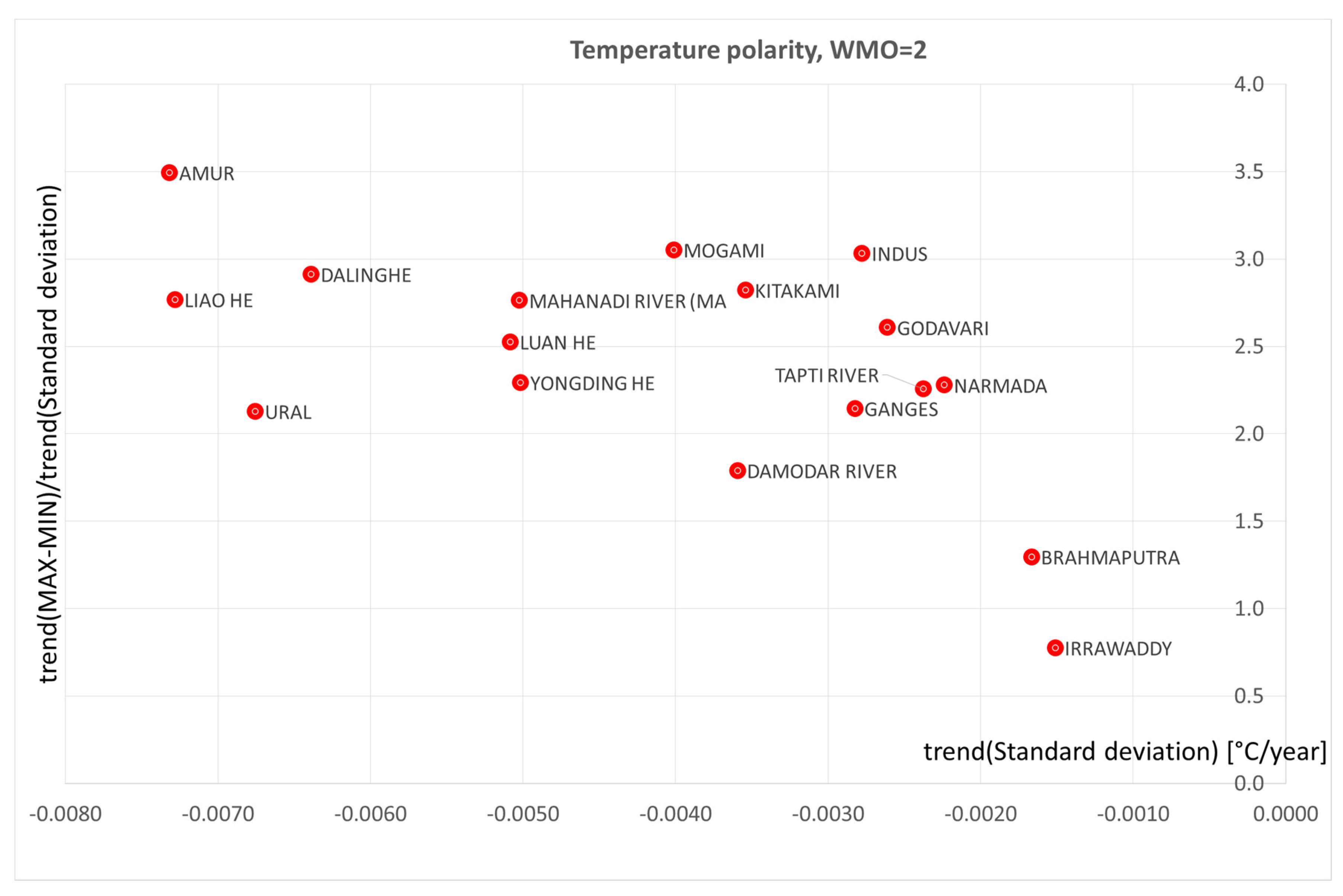
Figure 13.
Watersheds in the region for which WMO_REG=3, in which significant polarization trends were identified for monthly mean temperatures during the period from 1901 to 2010 at a significance level of 5%.
Figure 13.
Watersheds in the region for which WMO_REG=3, in which significant polarization trends were identified for monthly mean temperatures during the period from 1901 to 2010 at a significance level of 5%.
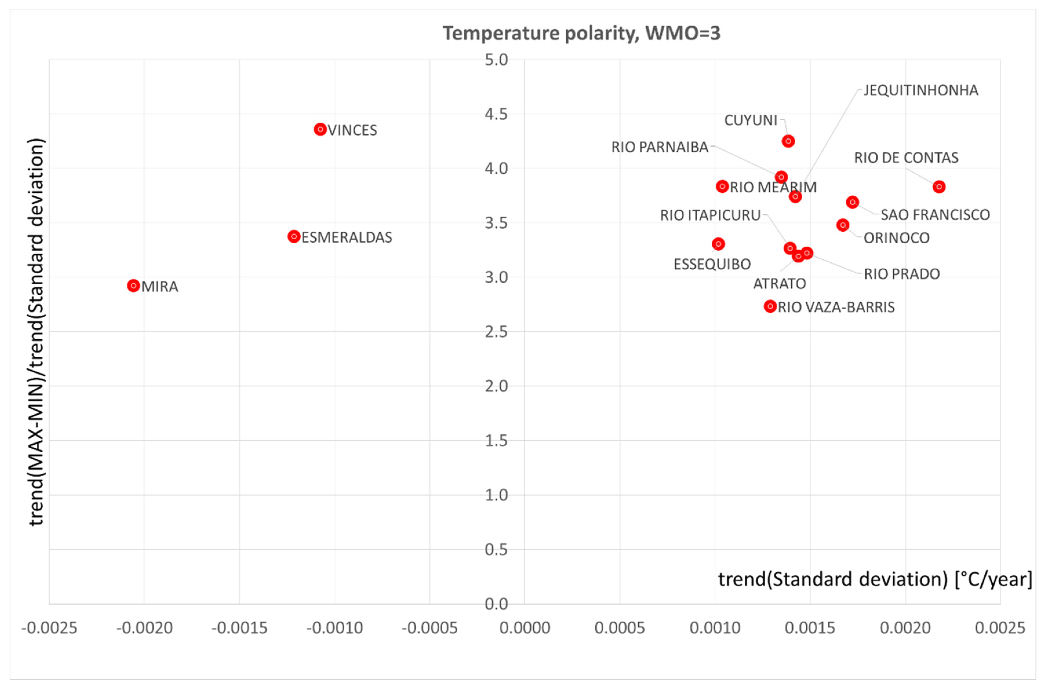
Figure 14.
Watersheds in the region for which WMO_REG=4, in which significant polarization trends were identified for monthly mean temperatures during the period from 1901 to 2010 at a significance level of 5%.
Figure 14.
Watersheds in the region for which WMO_REG=4, in which significant polarization trends were identified for monthly mean temperatures during the period from 1901 to 2010 at a significance level of 5%.
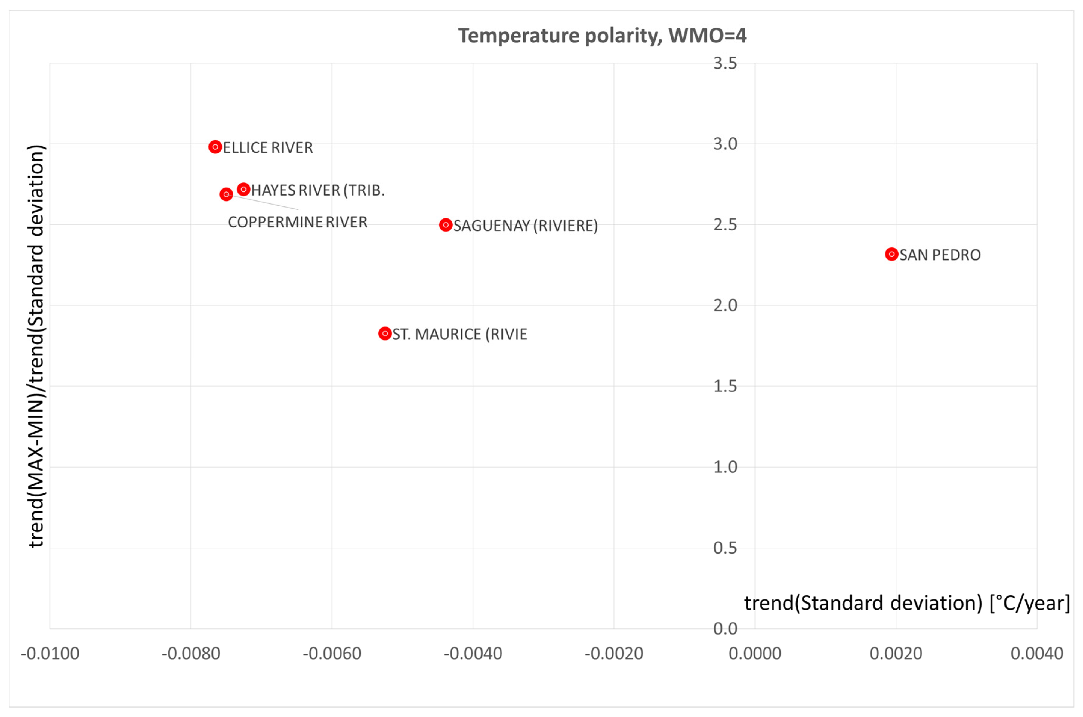
Figure 15.
Watersheds in the region for which WMO_REG=5, in which significant polarization trends were identified for monthly mean temperatures during the period from 1901 to 2010 at a significance level of 5%.
Figure 15.
Watersheds in the region for which WMO_REG=5, in which significant polarization trends were identified for monthly mean temperatures during the period from 1901 to 2010 at a significance level of 5%.
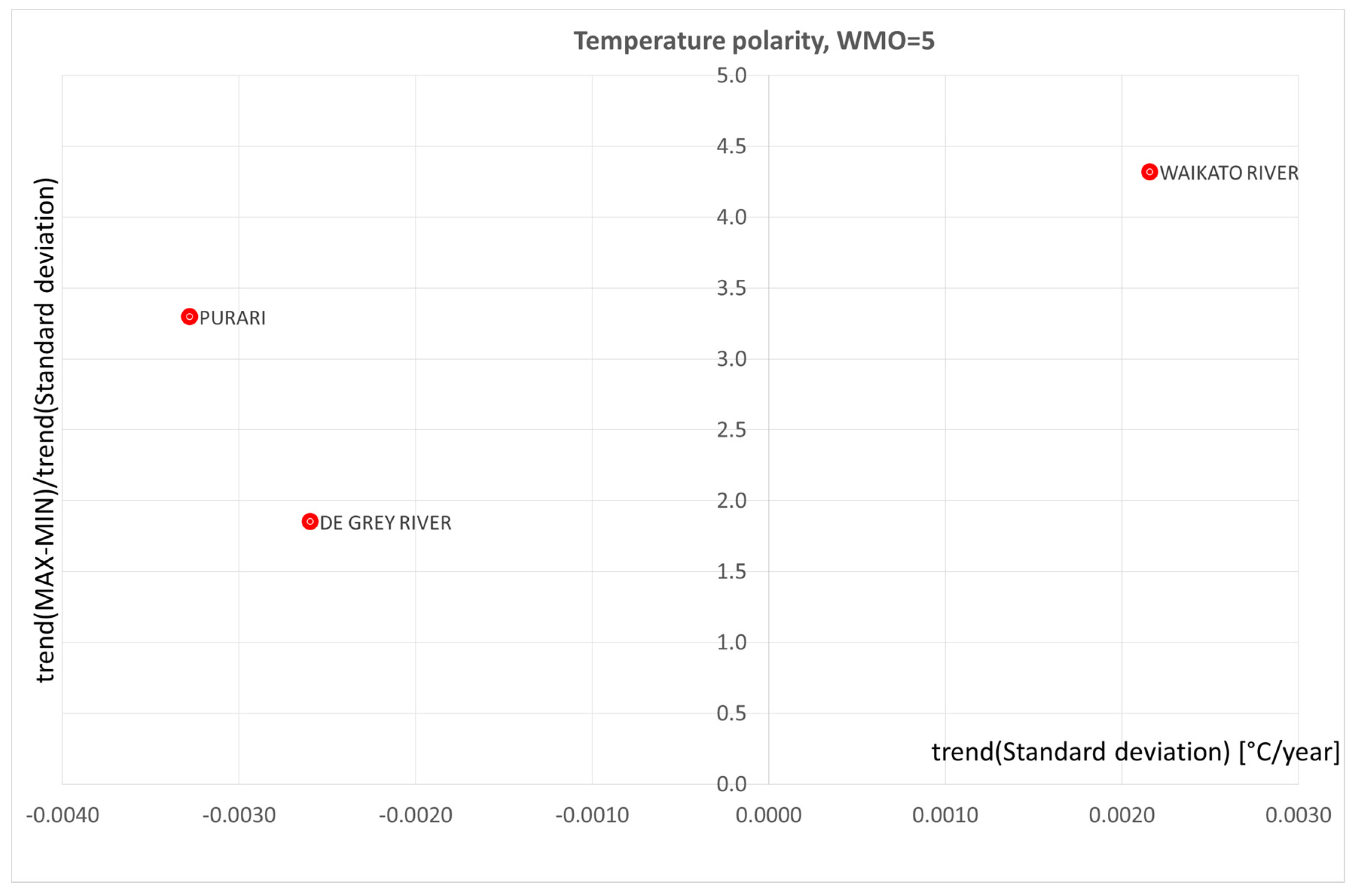
Figure 16.
Watersheds in the region for which WMO_REG=6, in which significant polarization trends were identified for monthly mean temperatures during the period from 1901 to 2010 at a significance level of 5%.
Figure 16.
Watersheds in the region for which WMO_REG=6, in which significant polarization trends were identified for monthly mean temperatures during the period from 1901 to 2010 at a significance level of 5%.
9. Conclusions
The article presents a multi-country analysis of monthly precipitation totals based on the GPCC database, and monthly mean temperatures (NOAA data) for 377 catchments distributed across the globe. Land area coverage reaches 13%. 110-year data sequences from 1901 to 2010 calculated from grid data with a spatial resolution of 0.5°x 0.5° longitude and latitude were analyzed. The data were analyzed in cross sections of calendar year months. In the study, 377 catchments x110 years x 12 months = 497640 precipitation data strings and as many temperature data strings were created and analyzed, for a total of about 1 million long-term strings characterizing climatic phenomena in the area of precipitation and temperature variability. Statistical characteristics in terms of calendar months were calculated and the min, max, standard deviation values were given. The indices of the adopted measures of polarization were calculated based on the factors of amplitude and standard deviation, and based on the trends of these characteristics. Non-parametric TMK and TP trends were used in the analysis.
The polarization index taking into account both precipitation and temperature phenomena is shown in Figure 17. On the horizontal axis is the polarization index of monthly precipitation totals, while on the vertical axis is the polarization index of monthly average temperatures. The points depicting the polarization phenomenon furthest from the center of the system indicate a high intensity of polarization. The highest values are found in the VINCES (South America) catchment with positive values of both trends of precipitation polarization factors and negative values of both trends of temperature polarization factors. This indicates an increase in precipitation factor anomalies. Calming of precipitation and temperature anomalies (negative trends in both precipitation and temperature factors) are expected in the BRAHMAPUTRA and YONGDING HE catchments. For the PURARI (Australia and Oceania) and MANGOKY - Africa catchments, calculations indicate a calming of anomalies in both the temperature and precipitation variability area. Temperature and precipitation anomalies are to be expected in the ATRATO: South America catchments.
In the calculations carried out in determining the polarity index, in addition to cases of trends with a concordant sign (both polarity factors positive or both negative), there were also cases where catchments showed opposite signs of trends in the polarity factors in both precipitation and temperature sequence analysis. However, adopting a 5% significance level for the MKT test resulted in the rejection of these cases. The concordance of the trend sign (max-min) and trend (STD) for precipitation is due to the fact that in most cases the variability of precipitation is correlated with changes in its maximum and minimum values. In other words, when there are periods of increased precipitation, we usually also observe higher maximum and minimum values of precipitation, and thus an increase in variability relative to the average value. Similarly, when there are periods of increased drought, there tend to be lower maximum and minimum values of precipitation, and variability relative to the average is also lower. However, it should be remembered that there are also periods when maximum and minimum values of precipitation may increase or decrease, but the variability relative to the average remains constant or changes in the opposite direction.
Analysis of temperature and precipitation polarities is necessary because of their impact on many aspects of the natural and human environment. Based on long-term sequences of precipitation and temperature, the article shows that the polarization process is present and can lead to significant changes in the local environment. Such changes can affect the distribution of plant and animal species, weather patterns, agriculture and the economy, and more. In addition, precipitation and temperature play a key role in the global energy and water cycles, and their variability can lead to floods, droughts and other natural disasters. For this reason, knowledge of the nature of changes and time scales is used to reduce the risk of floods and droughts. A proper understanding of the polarization of extreme events is also crucial for developing strategies related to mitigation and minimizing the impact of anthropogenic factors. The article shows the possibilities of assessing polarization in the area of precipitation variability and temperatures, which can help develop such strategies. The following climate changes suggest that polarization is becoming more entrenched, and the associated extremes are becoming more intense and unevenly distributed. Therefore, analysis of temperature and precipitation polarization is important for understanding climate change and its impact on our environment, as well as for developing effective strategies to manage risk and minimize human impact on the environment.
Funding
This research received no external funding.
Data Availability Statement
Data available upon request due to necessary commentary.
Conflicts of Interest
The author declare no conflict of interest.
References
- R. J. Romanowicz et al., “Climate Change Impact on Hydrological Extremes: Preliminary Results from the Polish-Norwegian Project,” Acta Geophys., vol. 64, no. 2, pp. 477–509, 2016. [CrossRef]
- S. Palaniswami and K. Muthiah, “Change point detection and trend analysis of rainfall and temperature series over the vellar river basin,” Polish J. Environ. Stud., vol. 27, no. 4, pp. 1673–1682, 2018. [CrossRef]
- D. G. Groves, D. Yates, and C. Tebaldi, “Developing and applying uncertain global climate change projections for regional water management planning,” Water Resour. Res., vol. 44, no. 12, pp. 1–16, 2008. [CrossRef]
- R. Katz, “Statistics of Extremes in Climatology and Hydrology,” Adv. Water Resour., vol. 25, pp. 1287–1304, 2002.
- R. W. Herschy, “The world’s maximum observed floods,” Flow Meas. Instrum., vol. 13, no. 5–6, pp. 231–235, 2002. [CrossRef]
- G. Blöschl et al., “Twenty-three unsolved problems in hydrology (UPH)–a community perspective,” Hydrol. Sci. J., vol. 64, no. 10, pp. 1141–1158, 2019. [CrossRef]
- S. C. Lewis and A. D. King, “Evolution of mean, variance and extremes in 21st century temperatures,” Weather Clim. Extrem., vol. 15, no. July 2016, pp. 1–10, 2017. [CrossRef]
- R. K. Jaiswal, A. K. Lohani, and H. L. Tiwari, “Statistical Analysis for Change Detection and Trend Assessment in Climatological Parameters,” Environ. Process., vol. 2, no. 4, pp. 729–749, 2015. [CrossRef]
- R. R. Heim, “An overview of weather and climate extremes - Products and trends,” Weather Clim. Extrem., vol. 10, pp. 1–9, 2015. [CrossRef]
- J. Sillmann et al., “Understanding, modeling and predicting weather and climate extremes: Challenges and opportunities,” Weather Clim. Extrem., vol. 18, no. August, pp. 65–74, 2017. [CrossRef]
- D. Młyński, M. Cebulska, and A. Wałȩga, “Trends, variability, and seasonality of maximum annual daily precipitation in the Upper Vistula Basin, Poland,” Atmosphere (Basel)., vol. 9, no. 8, pp. 1–14, 2018. [CrossRef]
- D. Młyński, A. Wałȩga, A. Petroselli, F. Tauro, and M. Cebulska, “Estimating maximum daily precipitation in the Upper Vistula Basin, Poland,” Atmosphere (Basel)., vol. 10, no. 2, 2019. [CrossRef]
- C. M. Twardosz R., “Temporal variability of maximum monthly precipitation totals in the Polish Western Carpathian Mts during the period 1951 – 2005,” pp. 123–134, 2012. [CrossRef]
- A. Ziernicka-Wojtaszek and J. Kopcińska, “Variation in atmospheric precipitation in Poland in the years 2001-2018,” Atmosphere (Basel)., vol. 11, no. 8, 2020. [CrossRef]
- N. Venegas-Cordero, Z. W. Kundzewicz, S. Jamro, and M. Piniewski, “Detection of trends in observed river floods in Poland,” J. Hydrol. Reg. Stud., vol. 41, Jun. 2022. [CrossRef]
- Z. W. Kundzewicz and M. Radziejewski, “Methodologies for trend detection,” IAHS-AISH Publ., no. 308, pp. 538–549, 2006.
- Z. W. Kundzewicz and A. Robson, “Detecting Trend and Other Changes in Hydrological Data,” World Clim. Program. - Water, no. May, p. 158, 2000, [Online]. Available: http://water.usgs.gov/osw/wcp-water/detecting-trend.pdf.
- T. Berezowski et al., “CPLFD-GDPT5: High-resolution gridded daily precipitation and temperature data set for two largest Polish river basins,” Earth Syst. Sci. Data, vol. 8, no. 1, pp. 127–139, 2016. [CrossRef]
- B. Twaróg, “Characteristics of multi-annual variation of precipitation in areas particularly exposed to extreme phenomena. Part 1. the upper Vistula river basin,” E3S Web Conf., vol. 49, 2018. [CrossRef]
- Y. Yu et al., “Climatic factors and human population changes in Eurasia between the Last Glacial Maximum and the early Holocene,” Glob. Planet. Change, vol. 221, p. 104054, Feb. 2023. [CrossRef]
- T. Chen, L. Zou, J. Xia, H. Liu, and F. Wang, “Decomposing the impacts of climate change and human activities on runoff changes in the Yangtze River Basin: Insights from regional differences and spatial correlations of multiple factors,” J. Hydrol., vol. 615, p. 128649, Dec. 2022. [CrossRef]
- E. Szolgayova, J. Parajka, G. Blöschl, and C. Bucher, “Long term variability of the Danube River flow and its relation to precipitation and air temperature,” J. Hydrol., vol. 519, no. PA, pp. 871–880, 2014. [CrossRef]
- I. G. Pechlivanidis, J. Olsson, T. Bosshard, D. Sharma, and K. C. Sharma, “Multi-basin modelling of future hydrological fluxes in the Indian subcontinent,” Water (Switzerland), vol. 8, no. 5, pp. 1–21, 2016. [CrossRef]
- M. Mudelsee, M. Börngen, G. Tetzlaff, and U. Grünewald, “Extreme floods in central Europe over the past 500 years: Role of cyclone pathway ‘Zugstrasse Vb,’” J. Geophys. Res. D Atmos., vol. 109, no. 23, pp. 1–21, 2004. [CrossRef]
- S. J. Vavrus, M. Notaro, and D. J. Lorenz, “Interpreting climate model projections of extreme weather events,” Weather Clim. Extrem., vol. 10, pp. 10–28, 2015. [CrossRef]
- O. Angélil et al., “Comparing regional precipitation and temperature extremes in climate model and reanalysis products,” Weather Clim. Extrem., vol. 13, pp. 35–43, 2016. [CrossRef]
- S. Michaelides, V. Levizzani, E. Anagnostou, P. Bauer, T. Kasparis, and J. E. Lane, “Precipitation: Measurement, remote sensing, climatology and modeling,” Atmos. Res., vol. 94, no. 4, pp. 512–533, Dec. 2009. [CrossRef]
- N. Das, R. Bhattacharjee, A. Choubey, A. Ohri, S. B. Dwivedi, and S. Gaur, “Time series analysis of automated surface water extraction and thermal pattern variation over the Betwa river, India,” Adv. Sp. Res., vol. 68, no. 4, pp. 1761–1788, Aug. 2021. [CrossRef]
- R. F. Reinking, “An approach to remote sensing and numerical modeling of orographic clouds and precipitation for climatic water resources assessment,” Atmos. Res., vol. 35, no. 2–4, pp. 349–367, Jan. 1995. [CrossRef]
- C. López-Bermeo, R. D. Montoya, F. J. Caro-Lopera, and J. A. Díaz-García, “Validation of the accuracy of the CHIRPS precipitation dataset at representing climate variability in a tropical mountainous region of South America,” Phys. Chem. Earth, Parts A/B/C, vol. 127, p. 103184, Oct. 2022. [CrossRef]
- A. Becker et al., “A description of the global land-surface precipitation data products of the Global Precipitation Climatology Centre with sample applications including centennial (trend) analysis from 1901-present,” Earth Syst. Sci. Data, vol. 5, no. 1, pp. 71–99, 2013. [CrossRef]
- J. D. Gómez, J. D. Etchevers, A. I. Monterroso, C. Gay, J. Campo, and M. Martínez, “Spatial estimation of mean temperature and precipitation in areas of scarce meteorological information,” Atmosfera, vol. 21, no. 1, pp. 35–56, 2008.
- D. R. Easterling, K. E. Kunkel, M. F. Wehner, and L. Sun, “Detection and attribution of climate extremes in the observed record,” Weather Clim. Extrem., vol. 11, pp. 17–27, 2016. [CrossRef]
- G. Guimares Nobre, B. Jongman, J. Aerts, and P. J. Ward, “The role of climate variability in extreme floods in Europe,” Environ. Res. Lett., vol. 12, no. 8, 2017. [CrossRef]
- T. Petrow and B. Merz, “Trends in flood magnitude, frequency and seasonality in Germany in the period 1951–2002,” J. Hydrol., vol. 371, no. 1–4, pp. 129–141, Jun. 2009. [CrossRef]
- P. Singh, A. Gupta, and M. Singh, “Hydrological inferences from watershed analysis for water resource management using remote sensing and GIS techniques,” Egypt. J. Remote Sens. Sp. Sci., vol. 17, no. 2, pp. 111–121, 2014. [CrossRef]
- X. Zhang, L. A. Vincent, W. D. Hogg, and A. Niitsoo, “Temperature and precipitation trends in Canada during the 20th century,” Atmos. - Ocean, vol. 38, no. 3, pp. 395–429, 2000. [CrossRef]
- N. N. Karmeshu Supervisor Frederick Scatena, “Trend Detection in Annual Temperature & Precipitation using the Mann Kendall Test – A Case Study to Assess Climate Change on Select States in the Northeastern United States,” Mausam, vol. 66, no. 1, pp. 1–6, 2015, [Online]. Available: http://repository.upenn.edu/mes_capstones/47.
- R. Dankers and R. Hiederer, “Extreme Temperatures and Precipitation in Europe: Analysis of a High-Resolution Climate Change Scenario,” JRC Sci. Tech. Reports, p. 82, 2008.
- R. W. Katz and M. B. Parlange, “Overdispersion phenomenon in stochastic modeling of precipitation,” J. Clim., vol. 11, no. 4, pp. 591–601, 1998. [CrossRef]
- S. Sen Roy and R. C. Balling, “Trends in extreme daily precipitation indices in India,” Int. J. Climatol., vol. 24, no. 4, pp. 457–466, 2004. [CrossRef]
- A. Colmet-Daage et al., “Evaluation of uncertainties in mean and extreme precipitation under climate change for northwestern Mediterranean watersheds from high-resolution Med and Euro-CORDEX ensembles,” Hydrol. Earth Syst. Sci., vol. 22, no. 1, pp. 673–687, 2018. [CrossRef]
- G. Y. Lenny Bernstein, Peter Bosch, Osvaldo Canziani, Zhenlin Chen, Renate Christ, Ogunlade Davidson, William Hare, Saleemul Huq, David Karoly, Vladimir Kattsov, Zbigniew Kundzewicz, Jian Liu, Ulrike Lohmann, Martin Manning, Taroh Matsuno, Bettina Menne, Bert M, “Climate Change 2007 : An Assessment of the Intergovernmental Panel on Climate Change,” Change, vol. 446, no. November, pp. 12–17, 2007, [Online]. Available: http://www.ipcc.ch/pdf/assessment-report/ar4/syr/ar4_syr.pdf.
- J. Chapman, “A nonparametric approach to detecting changes in variance in locally stationary time series,” no. April 2019, pp. 1–12, 2020. [CrossRef]
- M. H. and A. J. C. Philp K. Thornton, Pplly J. Ericksen, “Climate variability and vulnerability to climate change : A review,” pp. 3313–3328, 2014. [CrossRef]
- K. L. Swanson and A. A. Tsonis, “Has the climate recently shifted ?,” vol. 36, no. January, pp. 2–5, 2009. [CrossRef]
- S. Balhane, F. Driouech, O. Chafki, R. Manzanas, A. Chehbouni, and W. Moufouma-Okia, “Changes in mean and extreme temperature and precipitation events from different weighted multi-model ensembles over the northern half of Morocco,” Clim. Dyn., vol. 58, no. 1–2, pp. 389–404, 2022. [CrossRef]
- T. Mesbahzadeh, M. M. Miglietta, M. Mirakbari, F. Soleimani Sardoo, and M. Abdolhoseini, “Joint Modeling of Precipitation and Temperature Using Copula Theory for Current and Future Prediction under Climate Change Scenarios in Arid Lands (Case Study, Kerman Province, Iran),” Adv. Meteorol., vol. 2019, 2019. [CrossRef]
- D. Gerten, S. Rost, W. von Bloh, and W. Lucht, “Causes of change in 20th century global river discharge,” Geophys. Res. Lett., vol. 35, no. 20, pp. 1–5, 2008. [CrossRef]
- D. E. Walling, “Human impact on land–ocean sediment transfer by the world’s rivers,” Geomorphology, vol. 79, no. 3–4, pp. 192–216, Sep. 2006. [CrossRef]
- T. S. Hunter, A. H. Clites, K. B. Campbell, and A. D. Gronewold, “Development and application of a North American Great Lakes hydrometeorological database — Part I: Precipitation, evaporation, runoff, and air temperature,” J. Great Lakes Res., vol. 41, no. 1, pp. 65–77, Mar. 2015. [CrossRef]
- Y. Chai et al., “Homogenization and polarization of the seasonal water discharge of global rivers in response to climatic and anthropogenic effects,” Sci. Total Environ., vol. 709, p. 136062, 2020. [CrossRef]
- Z. Li, Y. Shi, A. A. Argiriou, P. Ioannidis, A. Mamara, and Z. Yan, “A Comparative Analysis of Changes in Temperature and Precipitation Extremes since 1960 between China and Greece,” Atmosphere (Basel)., vol. 13, no. 11, 2022. [CrossRef]
- M. Jahn, “Economics of extreme weather events: Terminology and regional impact models,” Weather Clim. Extrem., vol. 10, pp. 29–39, 2015. [CrossRef]
- X. Zhang et al., “Indices for monitoring changes in extremes based on daily temperature and precipitation data,” Wiley Interdiscip. Rev. Clim. Chang., vol. 2, no. 6, pp. 851–870, Nov. 2011. [CrossRef]
- R. P. Allan and B. J. Soden, “Atmospheric warming and the amplification of precipitation extremes,” Science (80-. )., vol. 321, no. 5895, pp. 1481–1484, 2008. [CrossRef]
- J. H. Christensen et al., “Climate phenomena and their relevance for future regional climate change,” Clim. Chang. 2013 Phys. Sci. Basis Work. Gr. I Contrib. to Fifth Assess. Rep. Intergov. Panel Clim. Chang., vol. 9781107057, pp. 1217–1308, 2013. [CrossRef]
- B. Rudolf, C. Beck, J. Grieser, and U. Schneider, “Global Precipitation Analysis Products of the GPCC,” Internet Pbulication, pp. 1–8, 2005, [Online]. Available: ftp://ftp-anon.dwd.de/pub/data/gpcc/PDF/GPCC_intro_products_2008.pdf.
- T. C. P. and R. S. Vose, “An overview of the global historical climatology network-daily database,” Bull. Am. Meteorol. Soc., vol. 78, no. 12, pp. 897–910, 1997. [CrossRef]
- M. G. Donat et al., “Updated analyses of temperature and precipitation extreme indices since the beginning of the twentieth century: The HadEX2 dataset,” J. Geophys. Res. Atmos., vol. 118, no. 5, pp. 2098–2118, 2013. [CrossRef]
- J. Persson et al., “No polarization-expected values of climate change impacts among European forest professionals and scientists,” Sustain., vol. 12, no. 7, 2020. [CrossRef]
- B. Arheimer et al., “Global catchment modelling using World-Wide HYPE (WWH), open data, and stepwise parameter estimation,” Hydrol. Earth Syst. Sci., vol. 24, no. 2, pp. 535–559, 2020. [CrossRef]
- L. R. Iverson and D. McKenzie, “Tree-species range shifts in a changing climate: Detecting, modeling, assisting,” Landsc. Ecol., vol. 28, no. 5, pp. 879–889, 2013. [CrossRef]
- J. Franklin, “Mapping Species Distributions: Spatial Inference and Prediction,” Oryx, vol. 44, no. 4, pp. 615–615, 2010. [CrossRef]
- D. Viner, M. Ekstrom, M. Hulbert, N. K. Warner, A. Wreford, and Z. Zommers, “Understanding the dynamic nature of risk in climate change assessments—A new starting point for discussion,” Atmos. Sci. Lett., vol. 21, no. 4, pp. 1–8, 2020. [CrossRef]
- M. Rosenzweig, C., Parry, “Potential impact of climate change on world food supply,” Nature, vol. 367, pp. 133–138, 1992. [CrossRef]
- T. M. Smith, R. W. Reynolds, T. C. Peterson, and J. Lawrimore, “Improvements to NOAA’s historical merged land-ocean surface temperature analysis (1880-2006),” J. Clim., vol. 21, no. 10, pp. 2283–2296, 2008. [CrossRef]
- A. Kosanic, K. Anderson, S. Harrison, T. Turkington, and J. Bennie, “Changes in the geographical distribution of plant species and climatic variables on the west cornwall peninsula (south west UK),” PLoS ONE, vol. 13, no. 2, pp. 1–18, 2018. [CrossRef]
- L. Chen and S. Guo, Copulas and its application in hydrology and water resources. 2019.
- W. Hou, P. Yan, G. Feng, and D. Zuo, “A 3D Copula Method for the Impact and Risk Assessment of Drought Disaster and an Example Application,” Front. Phys., vol. 9, no. April, pp. 1–14, 2021. [CrossRef]
- S. M. Ross, Introduction to Probability and Statistics, no. 5. Academic Press is an imprint ofElsevier, 2014.
- J. D. Santos-Gómez, J. S. Fontalvo-García, and J. D. Giraldo Osorio, “Validating the University of Delaware’s precipitation and temperature database for northern South America,” Dyna, vol. 82, no. 194, pp. 86–95, 2015. [CrossRef]
- Y. Amiel and F. Cowell, Thinking about Inequality, no. December 1999. 1999.
- M. O. Lorenz, “Methods of Measuring the Concentration of Wealth,” Publ. Am. Stat. Assoc., vol. 9, no. 70, pp. 209–219, 1905, [Online]. Available: https://www.jstor.org/stable/2276207. [CrossRef]
- M. G. and F. V. F. Francesco Nicolli, “Inequality and Climate Change: Two Problems, One Solution,” no. 2022, 2023, [Online]. Available: https://www.jstor.org/stable/resrep44832.
- T. Ogwang, “Calculating a standard error for the Gini coefficient: Some further results: Reply,” Oxf. Bull. Econ. Stat., vol. 66, no. 3, pp. 435–437, 2004. [CrossRef]
- C. Damgaard and J. Weiner, “Describing Inequality in Plant Size or Fecundity,” Ecology, vol. 81, no. 4, p. 1139, 2000. [CrossRef]
- T. Panek, “Polaryzacja ekonomiczna w Polsce,” Wiadomości Stat., vol. 1, no. 1, pp. 41–62, 2017.
- T. Sitthiyot and K. Holasut, “A simple method for measuring inequality,” Palgrave Commun., vol. 6, no. 1, pp. 1–9, 2020. [CrossRef]
- P.-M. Samson, Concentration of measure principle and entropy-inequalities. 2017.
- S. Yitzhaki, “Gini ’ s Mean Difference : A Superior Measure of Variability for Non-Normal Gini ’ s Mean difference : A superior measure of variability for non-normal distributions,” no. November, 2016.
- P. F. Pedro Conceição, “Young Person’s Guide to the Theil Index: Suggesting Intuitive Interpretations and Exploring Analytical Applications,” World, pp. 1–54, 2000, [Online]. Available: https://hal.science/hal-01365314. http://doi.org/10.2139/ssrn.228703.
- T. A. Buishand, “Some methods for testing the homogeneity of rainfall records,” J. Hydrol., vol. 58, no. 1–2, pp. 11–27, Aug. 1982. [CrossRef]
- A. K. Gupta, Jie Chen, “Parametric Statistical Change Point Analysis,” Angew. Chemie Int. Ed. 6(11), 951–952., pp. 2013–2015, 2021. [CrossRef]
- M. Radziejewski, A. Bardossy, and Z. W. Kundzewicz, “Détection de changements dans les séries de débits utilisant la randonisation de phase,” Hydrol. Sci. J., vol. 45, no. 4, pp. 547–558, 2000. [CrossRef]
- M. Salarijazi, “Trend and change-point detection for the annual stream-flow series of the Karun River at the Ahvaz hydrometric station,” African J. Agric. Reseearch, vol. 7, no. 32, pp. 4540–4552, 2012. [CrossRef]
- A. N. Pettitt, “A Non-Parametric Approach to the Change-Point Problem,” J. R. Stat. Soc. Ser. C (Applied Stat., vol. 28, no. 2, pp. 126–135, Apr. 1979. [CrossRef]
- G. Verstraeten, J. Poesen, G. Demarée, and C. Salles, “Long-term (105 years) variability in rain erosivity as derived from 10-min rainfall depth data for Ukkel (Brussels, Belgium): Implications for assessing soil erosion rates,” J. Geophys. Res. Atmos., vol. 111, no. 22, pp. 1–11, 2006. [CrossRef]
- L. C. Conte, D. M. Bayer, and F. M. Bayer, “Bootstrap Pettitt test for detecting change points in hydroclimatological data: Case study of Itaipu Hydroelectric Plant, Brazil,” Hydrol. Sci. J., vol. 64, no. 11, pp. 1312–1326, 2019. [CrossRef]
- H. B. Mann, “Nonparametric Tests Against Trend,” Econometrica, vol. 13, no. 3, pp. 245–259, Apr. 1945. [CrossRef]
- S. Yue, P. Pilon, B. Phinney, and G. Cavadias, “The influence of autocorrelation on the ability to detect trend in hydrological series,” Hydrol. Process., vol. 16, no. 9, pp. 1807–1829, 2002. [CrossRef]
- K. Sen, “Estimates of the Regression Coefficient Based on Kendall’s Tau,” J. Am. Stat. Assoc., vol. 63, no. 324, pp. 1379–1389, Dec. 1968. [CrossRef]
- M. Hirsch, J. R. Slack, and R. A. Smith, “Techniques of trend analysis for monthly water quality data,” Water Resour. Res., vol. 18, no. 1, pp. 107–121, Feb. 1982. [CrossRef]
Figure 1.
Watersheds in which significant polarization trends were identified for monthly precipitation sums during the period from 1901 to 2010 at a significance level of 5%.
Figure 1.
Watersheds in which significant polarization trends were identified for monthly precipitation sums during the period from 1901 to 2010 at a significance level of 5%.
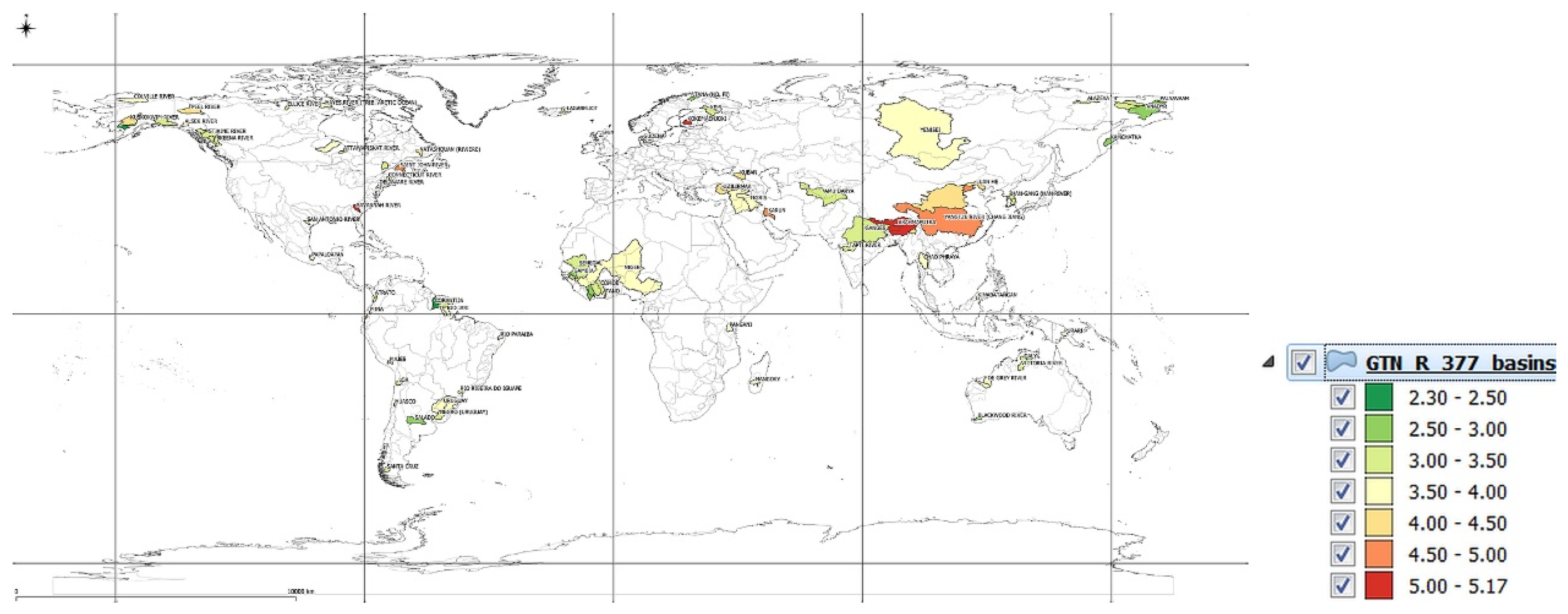
Figure 2.
Watersheds in which change points in the trend of factors related to precipitation polarization for monthly precipitation sums during the period from 1901 to 2010 were identified at a significance level of 5%.
Figure 2.
Watersheds in which change points in the trend of factors related to precipitation polarization for monthly precipitation sums during the period from 1901 to 2010 were identified at a significance level of 5%.
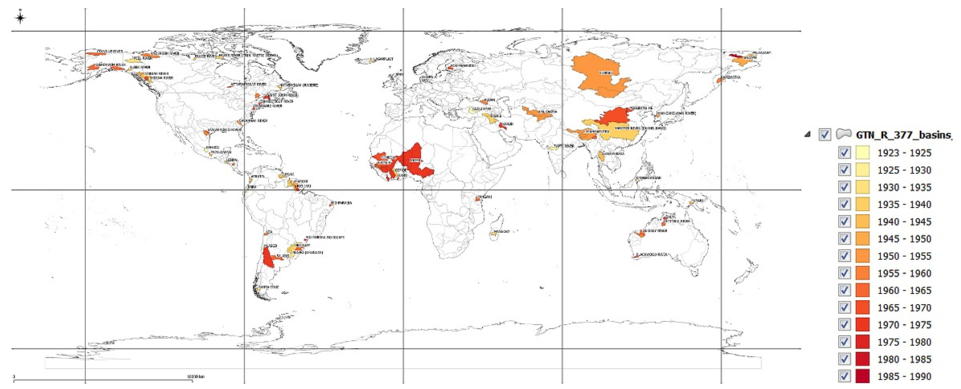
Figure 3.
Watersheds in the region for which WMO_REG=1, in which significant polarization trends were identified for monthly precipitation sums during the period from 1901 to 2010 at a significance level of 5%.
Figure 3.
Watersheds in the region for which WMO_REG=1, in which significant polarization trends were identified for monthly precipitation sums during the period from 1901 to 2010 at a significance level of 5%.
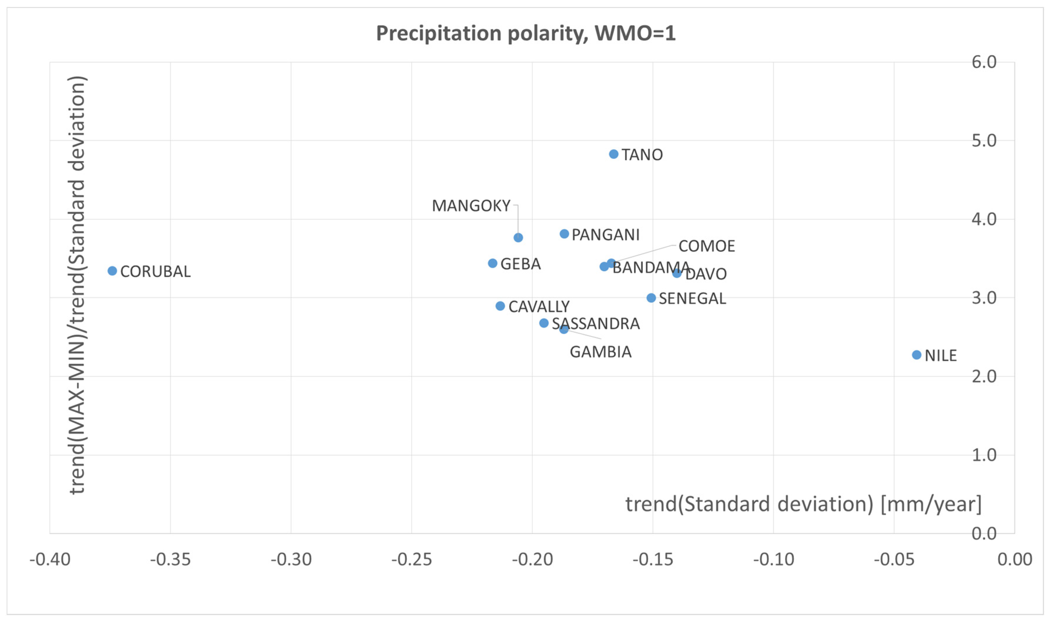
Figure 4.
Watersheds in the region for which WMO_REG=2, in which significant polarization trends were identified for monthly precipitation sums during the period from 1901 to 2010 at a significance level of 5%.
Figure 4.
Watersheds in the region for which WMO_REG=2, in which significant polarization trends were identified for monthly precipitation sums during the period from 1901 to 2010 at a significance level of 5%.
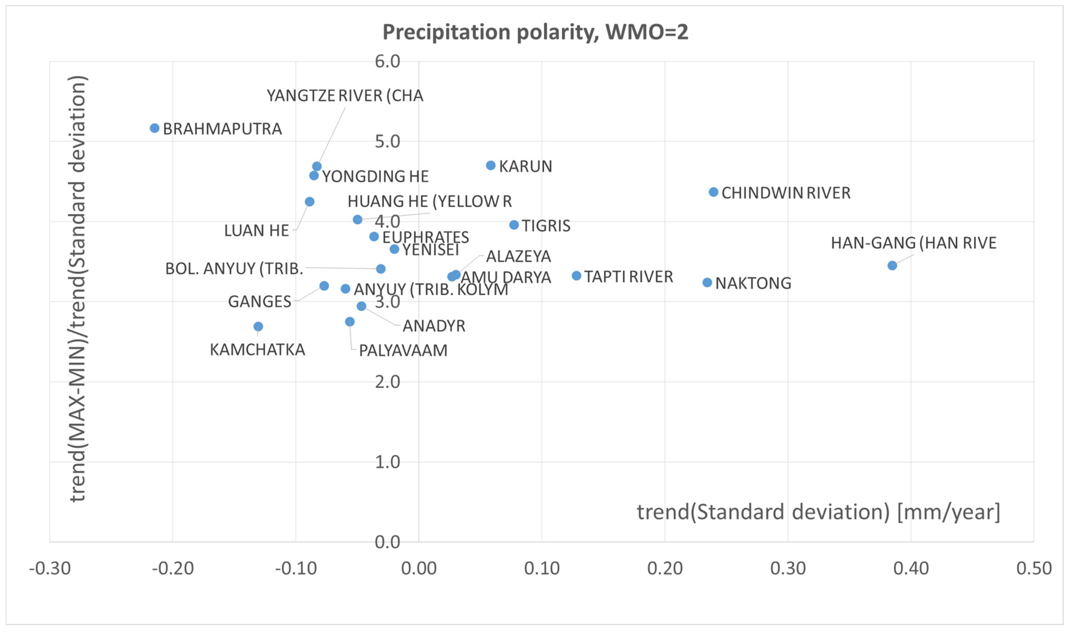
Figure 5.
Watersheds in the region for which WMO_REG=3, in which significant polarization trends were identified for monthly precipitation sums during the period from 1901 to 2010 at a significance level of 5%.
Figure 5.
Watersheds in the region for which WMO_REG=3, in which significant polarization trends were identified for monthly precipitation sums during the period from 1901 to 2010 at a significance level of 5%.
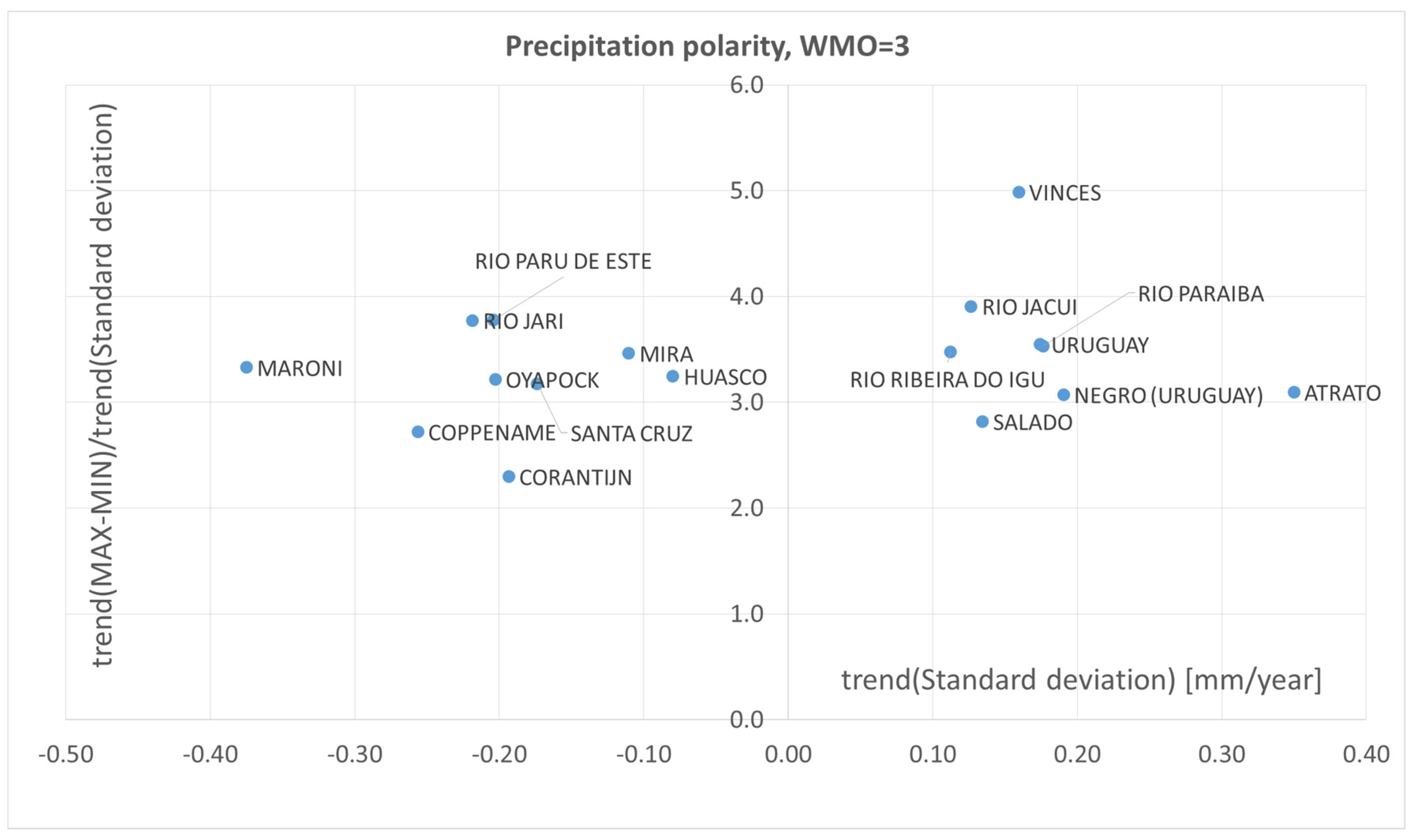
Figure 6.
Watersheds in the region for which WMO_REG=4, in which significant polarization trends were identified for monthly precipitation sums during the period from 1901 to 2010 at a significance level of 5%.
Figure 6.
Watersheds in the region for which WMO_REG=4, in which significant polarization trends were identified for monthly precipitation sums during the period from 1901 to 2010 at a significance level of 5%.
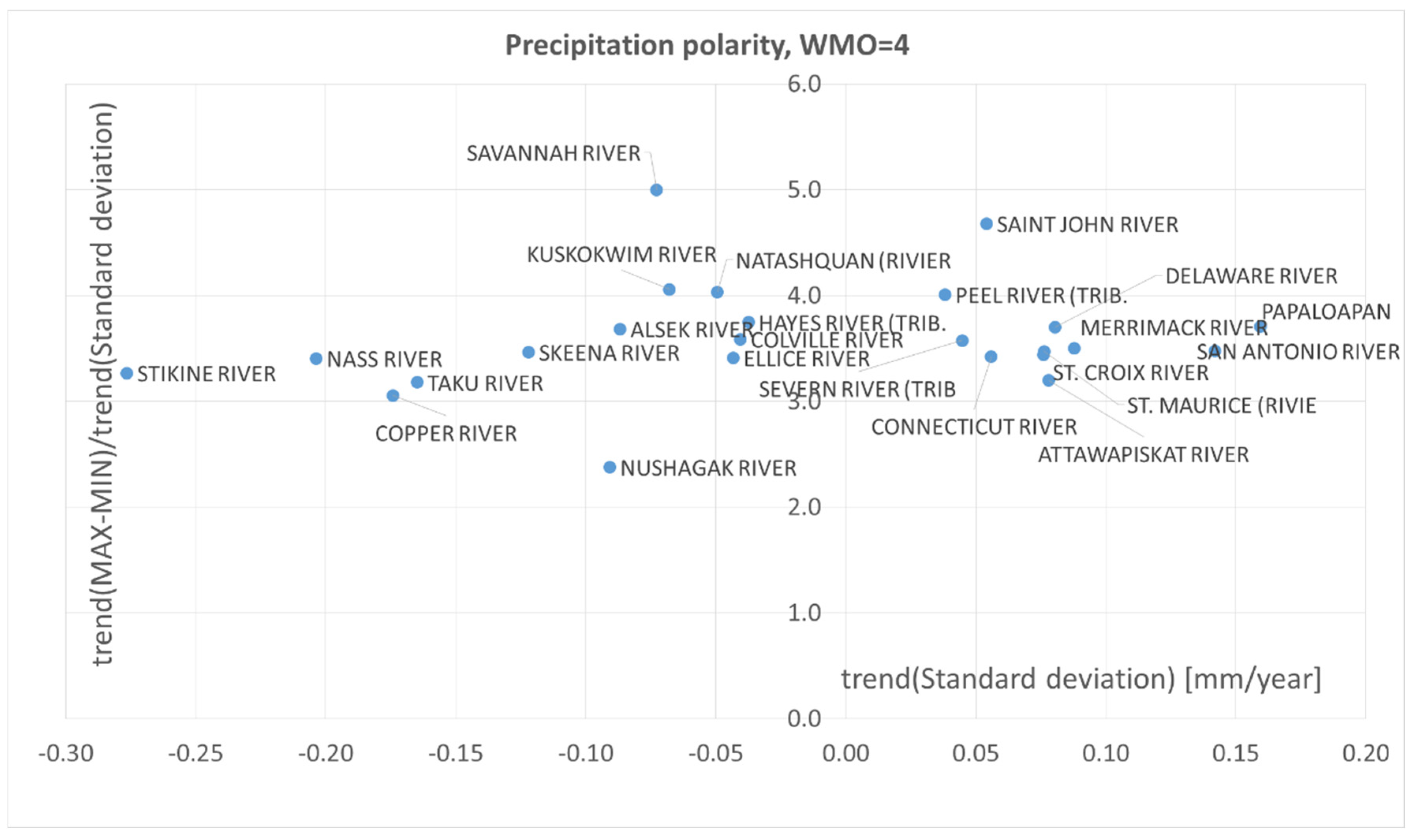
Figure 7.
Watersheds in the region for which WMO_REG=5, in which significant polarization trends were identified for monthly precipitation sums during the period from 1901 to 2010 at a significance level of 5%.
Figure 7.
Watersheds in the region for which WMO_REG=5, in which significant polarization trends were identified for monthly precipitation sums during the period from 1901 to 2010 at a significance level of 5%.
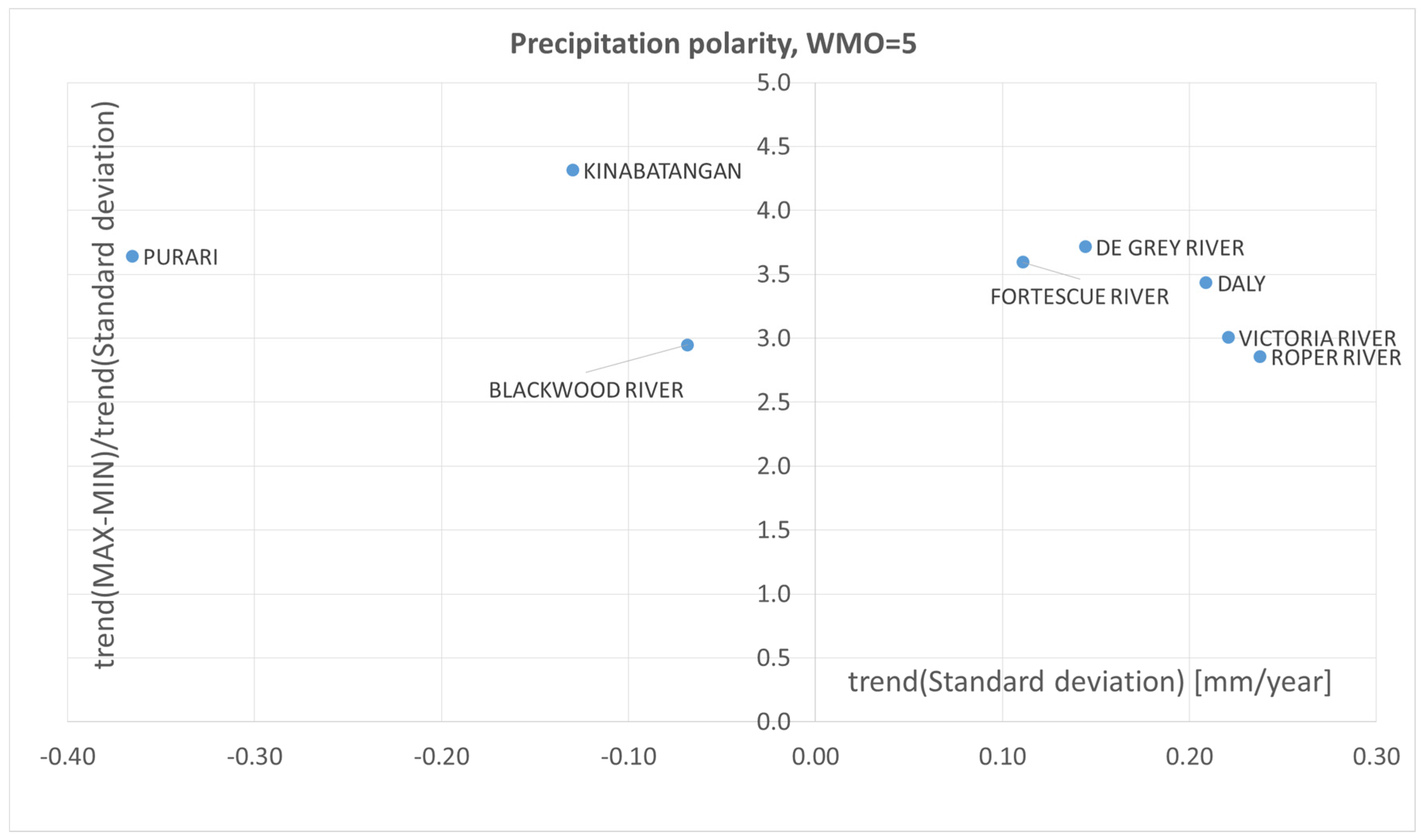
Figure 8.
Watersheds in the region for which WMO_REG=6, in which significant polarization trends were identified for monthly precipitation sums during the period from 1901 to 2010 at a significance level of 5%.
Figure 8.
Watersheds in the region for which WMO_REG=6, in which significant polarization trends were identified for monthly precipitation sums during the period from 1901 to 2010 at a significance level of 5%.
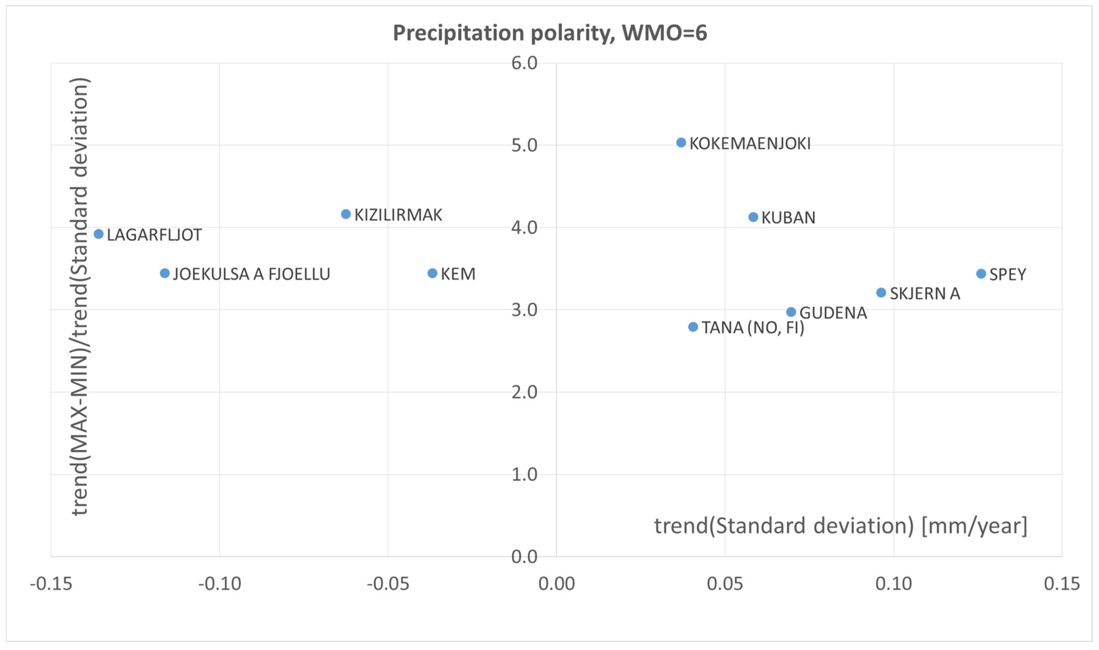
Figure 17.
A picture of polarization phenomena in the area of precipitation and temperature, taking into account WMO regions.
Figure 17.
A picture of polarization phenomena in the area of precipitation and temperature, taking into account WMO regions.
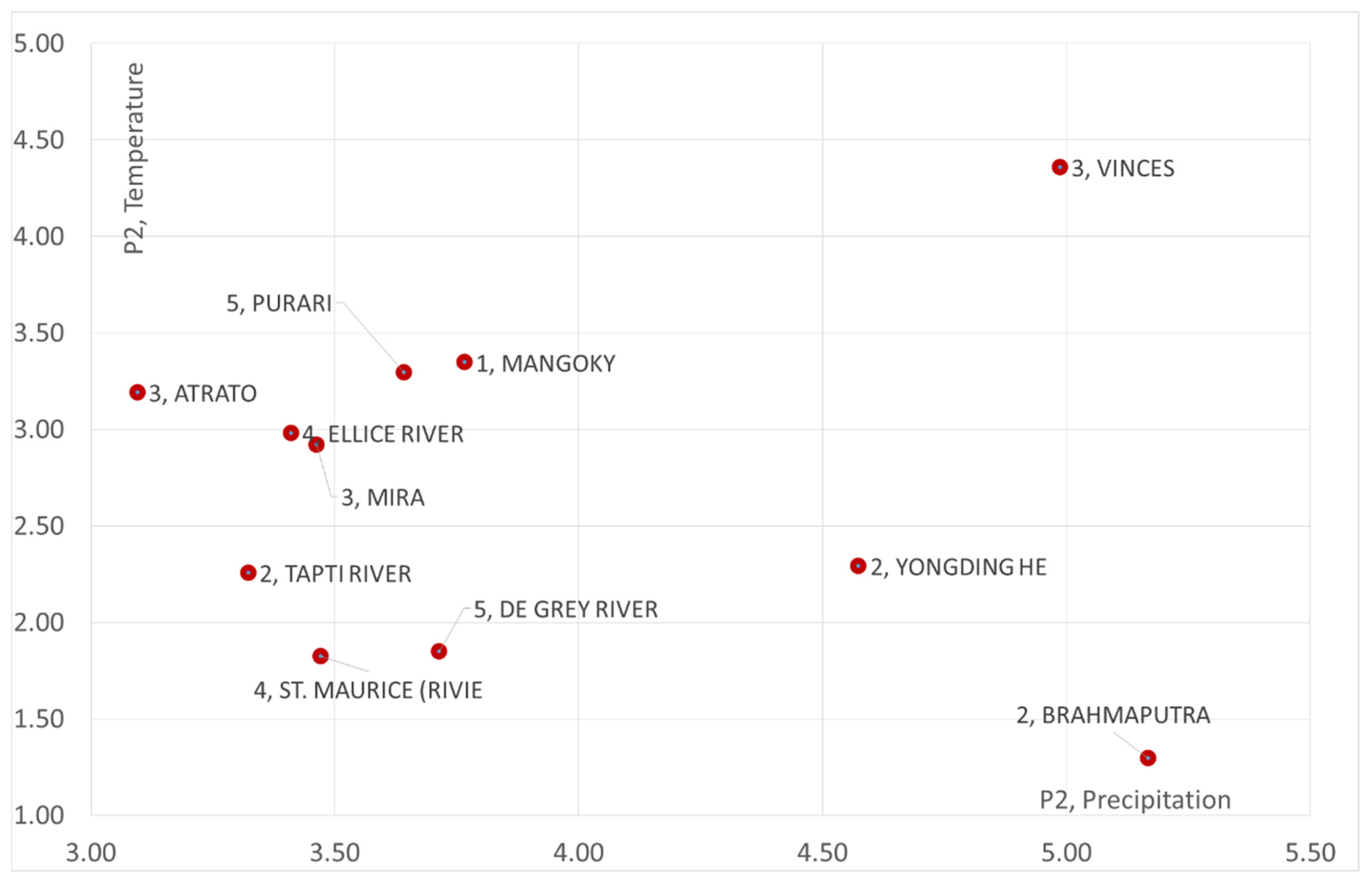

Table 1.
Areas covered by the analysis.
| Region | Continent | Lands area | Area catchment | Coverage of the continents |
| WMO | 106 km2 | 106 km2 | % | |
| 2 | Asia | 44.3 | 20.3 | 45.86% |
| 1 | Africa | 30.3 | 8.43 | 27.83% |
| 4 | North America | 24.2 | 13.0 | 53.87% |
| 3 | South America | 17.8 | 12.6 | 70.57% |
| Antarctica | 13.1 | 0.0 | 0.00% | |
| 6 | Europe | 10.5 | 6.7 | 64.10% |
| 5 | Australia and Oceania | 8.5 | 1.1 | 13.07% |
| Lands together | 148.7 | 65.1 | 43.77% | |
| Earth, total | 509.9 | 65.1 | 12.76% |
Table 2.
Characteristics calculated based on monthly precipitation sums in analyzed watersheds in terms of precipitation polarization.
Table 2.
Characteristics calculated based on monthly precipitation sums in analyzed watersheds in terms of precipitation polarization.
| No | GRDC | WMO | RIVER | COUNTRY | AREA | JAN | FEB | MAR | APR | MAY | JUN | JUL | AUG | SEP | OCT | NOV | DEC | MIN | MAX | MEAN | STD |
| 1 | 1104150 | 1 | CHELIF | DZ | 43750 | 54.9 | 43.2 | 41.0 | 37.8 | 34.1 | 11.3 | 3.8 | 7.4 | 26.8 | 40.3 | 48.3 | 56.0 | 0.2 | 209.6 | 33.7 | 30.54 |
| 2 | 1147010 | 1 | CONGO | CD | 3475000 | 122.7 | 123.2 | 158.3 | 152.1 | 105.9 | 71.0 | 70.2 | 97.6 | 129.9 | 161.9 | 163.5 | 146.5 | 45.2 | 227.2 | 125.2 | 36.04 |
| 3 | 1159100 | 1 | ORANGE | ZA | 850530 | 58.5 | 59.4 | 56.9 | 31.4 | 13.5 | 6.7 | 5.2 | 7.0 | 11.6 | 26.9 | 38.0 | 44.8 | 0.2 | 166.1 | 30.0 | 27.57 |
| 4 | 1160580 | 1 | GROOT-VIS | ZA | 29745 | 50.5 | 58.3 | 65.2 | 38.8 | 24.9 | 17.0 | 15.9 | 19.9 | 27.5 | 40.2 | 47.9 | 46.9 | 0.5 | 226.6 | 37.8 | 30.28 |
| 5 | 1160880 | 1 | TUGELA | ZA | 28920 | 147.7 | 127.5 | 102.6 | 46.1 | 20.6 | 12.5 | 13.1 | 23.0 | 41.2 | 83.4 | 113.0 | 131.5 | 0.2 | 351.2 | 71.9 | 60.10 |
| 6 | 1286900 | 1 | RUFIJI | TZ | 158200 | 176.3 | 154.7 | 196.3 | 155.0 | 41.8 | 7.9 | 5.1 | 4.1 | 6.2 | 15.3 | 55.9 | 152.7 | 0.1 | 380.9 | 80.9 | 84.20 |
| 7 | 1289200 | 1 | PANGANI | TZ | 25110 | 68.9 | 74.1 | 115.9 | 197.3 | 124.1 | 33.2 | 20.0 | 19.2 | 20.6 | 37.3 | 78.5 | 82.3 | 1.2 | 436.6 | 72.6 | 69.59 |
| 8 | 1289450 | 1 | RUVU | TZ | 15190 | 113.9 | 101.3 | 181.6 | 250.1 | 107.4 | 31.0 | 20.9 | 19.2 | 36.1 | 53.2 | 98.6 | 119.5 | 0.0 | 695.0 | 94.4 | 83.42 |
| 9 | 1309700 | 1 | SEBOU | MA | 17250 | 78.2 | 81.1 | 77.7 | 72.4 | 41.0 | 17.1 | 4.0 | 5.8 | 20.6 | 53.3 | 82.9 | 94.5 | 0.1 | 287.0 | 52.4 | 51.53 |
| 10 | 1336500 | 1 | CROSS | CM | 6810 | 23.9 | 51.3 | 144.4 | 194.9 | 241.0 | 311.6 | 379.4 | 398.6 | 425.5 | 312.4 | 90.5 | 25.0 | 0.0 | 1085.2 | 216.5 | 164.78 |
| 11 | 1338050 | 1 | SANAGA | CM | 131520 | 13.0 | 24.4 | 89.9 | 144.1 | 193.2 | 188.0 | 205.0 | 237.2 | 280.7 | 246.0 | 61.8 | 15.0 | 0.0 | 478.2 | 141.5 | 101.62 |
| 12 | 1339100 | 1 | NYONG | CM | 26400 | 29.8 | 51.4 | 135.6 | 178.5 | 224.5 | 160.6 | 96.3 | 136.0 | 265.5 | 303.0 | 127.0 | 36.4 | 0.0 | 1064.1 | 145.4 | 100.71 |
| 13 | 1340500 | 1 | NTEM | CM | 18100 | 50.8 | 72.3 | 152.4 | 182.1 | 198.2 | 123.1 | 56.1 | 63.4 | 212.0 | 281.4 | 166.5 | 61.3 | 0.0 | 1067.8 | 135.0 | 95.45 |
| 14 | 1362100 | 1 | NILE | EG | 2900000 | 10.3 | 13.9 | 27.1 | 45.9 | 64.1 | 74.5 | 110.9 | 123.9 | 86.3 | 52.0 | 26.0 | 14.7 | 3.3 | 167.5 | 54.2 | 38.6 |
| 15 | 1389090 | 1 | MANGOKY | MG | 53225 | 229.6 | 178.8 | 90.7 | 41.7 | 22.5 | 11.8 | 12.1 | 10.9 | 16.3 | 31.9 | 85.5 | 161.0 | 0.0 | 562.4 | 74.4 | 92.63 |
| 16 | 1389230 | 1 | TSIRIBIHINA | MG | 45000 | 293.6 | 215.3 | 142.3 | 58.7 | 24.7 | 12.1 | 14.2 | 12.6 | 18.0 | 48.3 | 107.0 | 198.6 | 0.0 | 613.7 | 95.5 | 110.17 |
| 17 | 1425500 | 1 | CAVALLY | CI | 28800 | 31.9 | 69.1 | 144.0 | 173.2 | 228.5 | 274.1 | 154.5 | 177.9 | 296.3 | 245.2 | 126.6 | 59.3 | 1.2 | 672.2 | 165.0 | 102.46 |
| 18 | 1426380 | 1 | BANDAMA | CI | 95500 | 12.3 | 32.4 | 80.5 | 117.4 | 142.3 | 153.8 | 129.8 | 159.0 | 192.3 | 123.5 | 40.7 | 16.6 | 0.0 | 434.6 | 100.1 | 71.48 |
| 19 | 1427500 | 1 | SASSANDRA | CI | 62000 | 14.2 | 40.8 | 96.6 | 130.3 | 154.1 | 185.4 | 175.4 | 222.9 | 250.6 | 157.2 | 52.5 | 18.5 | 0.0 | 624.8 | 124.9 | 90.50 |
| 20 | 1427600 | 1 | DAVO | CI | 6600 | 26.9 | 60.7 | 131.0 | 153.1 | 184.9 | 207.8 | 93.8 | 93.3 | 172.9 | 153.9 | 89.0 | 39.4 | 0.0 | 597.4 | 117.2 | 77.62 |
| 21 | 1428500 | 1 | COMOE | CI | 69900 | 6.8 | 20.0 | 58.4 | 104.0 | 136.8 | 150.1 | 147.2 | 177.8 | 187.4 | 115.3 | 33.6 | 9.4 | 0.0 | 388.7 | 95.6 | 73.07 |
| 22 | 1445100 | 1 | KOUILOU | CG | 55010 | 160.5 | 150.9 | 192.5 | 203.9 | 126.1 | 7.7 | 2.2 | 4.9 | 19.7 | 119.5 | 251.4 | 192.7 | 0.0 | 467.0 | 119.3 | 98.86 |
| 23 | 1526300 | 1 | PRA | GH | 22714 | 20.3 | 59.9 | 124.2 | 146.6 | 182.1 | 221.1 | 119.8 | 73.2 | 153.5 | 175.3 | 91.9 | 38.4 | 0.0 | 428.0 | 117.2 | 74.41 |
| 24 | 1530100 | 1 | TANO | GH | 15800 | 19.6 | 53.3 | 119.1 | 140.1 | 201.9 | 253.5 | 125.8 | 73.7 | 155.9 | 177.6 | 91.1 | 38.5 | 0.0 | 568.5 | 120.8 | 86.63 |
| 25 | 1531700 | 1 | VOLTA | GH | 394100 | 3.6 | 10.3 | 32.6 | 64.8 | 101.9 | 136.4 | 167.4 | 207.6 | 182.3 | 80.4 | 16.6 | 6.2 | 0.0 | 333.8 | 84.2 | 74.34 |
| 26 | 1643100 | 1 | OGOOUE | GA | 205000 | 120.8 | 135.6 | 202.3 | 200.2 | 185.3 | 52.2 | 17.1 | 28.4 | 118.8 | 267.1 | 249.9 | 151.6 | 0.4 | 770.6 | 144.1 | 90.22 |
| 27 | 1644100 | 1 | NYANGA | GA | 20000 | 164.0 | 162.4 | 200.6 | 192.2 | 108.3 | 6.4 | 1.6 | 2.5 | 18.7 | 162.2 | 278.9 | 192.0 | 0.0 | 562.6 | 124.2 | 110.57 |
| 28 | 1732100 | 1 | MONO | BJ | 21575 | 10.8 | 26.5 | 73.0 | 113.0 | 141.1 | 165.5 | 178.2 | 174.9 | 195.0 | 116.7 | 25.5 | 14.3 | 0.1 | 370.9 | 102.9 | 77.29 |
| 29 | 1733600 | 1 | OUEME | BJ | 46990 | 7.1 | 15.2 | 50.1 | 92.7 | 137.8 | 157.3 | 179.8 | 184.9 | 194.0 | 108.5 | 16.4 | 6.2 | 0.0 | 404.4 | 95.8 | 80.01 |
| 30 | 1789300 | 1 | TANA | KE | 42220 | 34.4 | 25.8 | 77.8 | 181.4 | 76.3 | 17.9 | 14.4 | 15.9 | 15.2 | 82.2 | 168.3 | 77.2 | 2.5 | 527.0 | 65.6 | 73.02 |
| 31 | 1812100 | 1 | SENEGAL | SN | 268000 | 0.7 | 0.9 | 1.8 | 6.1 | 21.9 | 65.2 | 128.4 | 178.6 | 118.5 | 34.5 | 4.2 | 1.5 | 0.0 | 310.4 | 46.9 | 62.73 |
| 32 | 1813200 | 1 | GAMBIA | SN | 42000 | 0.6 | 0.9 | 2.5 | 7.7 | 44.9 | 151.1 | 240.1 | 314.0 | 259.8 | 90.9 | 12.8 | 2.0 | 0.0 | 482.6 | 93.9 | 117.80 |
| 33 | 1814070 | 1 | GEBA | SN | 7340 | 0.3 | 0.7 | 0.4 | 1.8 | 25.8 | 137.9 | 225.4 | 343.0 | 287.0 | 106.0 | 9.1 | 0.9 | 0.0 | 653.1 | 94.9 | 128.2 |
| 34 | 1815020 | 1 | CORUBAL | SN | 23840 | 0.9 | 1.5 | 4.4 | 16.2 | 70.8 | 205.9 | 324.4 | 429.2 | 364.3 | 172.0 | 33.6 | 4.1 | 0.0 | 796.7 | 135.6 | 160.32 |
| 35 | 1834101 | 1 | NIGER | NG | 575500 | 1.6 | 2.4 | 10.0 | 27.5 | 58.0 | 85.7 | 133.1 | 169.2 | 118.0 | 43.0 | 5.9 | 1.6 | 0.1 | 236.1 | 54.7 | 57.78 |
| 36 | 1878100 | 1 | SHEBELLE | SO | 278000 | 9.0 | 16.7 | 38.5 | 105.4 | 93.7 | 35.5 | 49.8 | 63.4 | 58.1 | 85.4 | 39.0 | 9.8 | 0.2 | 268.1 | 50.4 | 39.91 |
| 37 | 1880100 | 1 | JUBA | SO | 179520 | 10.9 | 18.3 | 50.1 | 142.6 | 111.9 | 30.1 | 35.6 | 43.1 | 61.6 | 108.6 | 48.8 | 14.2 | 0.2 | 396.8 | 56.3 | 49.87 |
| 38 | 1891500 | 1 | ZAMBEZI | MZ | 940000 | 208.8 | 183.3 | 141.2 | 39.8 | 6.0 | 1.3 | 0.6 | 1.1 | 4.7 | 28.5 | 101.4 | 190.5 | 0.1 | 390.0 | 75.6 | 84.92 |
| 39 | 1894200 | 1 | BUZI | MZ | 26314 | 240.1 | 215.0 | 174.1 | 58.3 | 24.7 | 19.8 | 17.9 | 17.0 | 19.1 | 43.4 | 107.8 | 195.1 | 0.6 | 769.3 | 94.4 | 107.3 |
| 40 | 1895500 | 1 | SAVE | MZ | 100885 | 152.1 | 136.7 | 97.6 | 32.2 | 12.4 | 8.9 | 7.1 | 5.7 | 9.9 | 29.2 | 82.6 | 138.8 | 0.2 | 589.7 | 59.4 | 75.1 |
| 41 | 1896500 | 1 | LIMPOPO | MZ | 342000 | 105.6 | 89.2 | 67.7 | 29.0 | 11.3 | 5.2 | 4.1 | 4.4 | 11.7 | 37.0 | 74.0 | 91.1 | 0.1 | 344.5 | 44.2 | 48.27 |
| 42 | 1897500 | 1 | INCOMATI | MZ | 37600 | 137.7 | 124.4 | 100.4 | 48.3 | 19.7 | 10.9 | 10.6 | 12.2 | 29.9 | 63.2 | 111.4 | 124.6 | 0.0 | 504.0 | 66.1 | 64.89 |
| 43 | 1899100 | 1 | MAPUTO | MZ | 28500 | 132.7 | 110.3 | 91.4 | 47.4 | 20.3 | 12.4 | 11.6 | 16.4 | 36.0 | 80.0 | 117.1 | 129.3 | 0.1 | 462.8 | 67.1 | 62.04 |
| 44 | 1992900 | 1 | SHIRE | MW | 149500 | 236.8 | 209.6 | 218.0 | 125.7 | 38.6 | 13.6 | 9.9 | 8.3 | 7.6 | 15.0 | 72.1 | 191.1 | 1.0 | 390.7 | 95.5 | 97.09 |
| 45 | 2178300 | 2 | YONGDING HE | CN | 42500 | 3.0 | 3.6 | 10.2 | 16.7 | 33.2 | 56.0 | 111.7 | 87.4 | 50.7 | 19.1 | 8.5 | 2.8 | 0.1 | 249.5 | 33.6 | 42.12 |
| 46 | 2178400 | 2 | DALINGHE | CN | 17687 | 2.1 | 2.8 | 8.6 | 19.3 | 42.7 | 80.2 | 148.2 | 120.3 | 46.9 | 23.8 | 8.3 | 3.2 | 0.0 | 474.1 | 42.2 | 58.50 |
| 47 | 2178500 | 2 | LUAN HE | CN | 44100 | 2.7 | 3.2 | 8.6 | 16.4 | 37.3 | 71.3 | 142.6 | 109.0 | 50.7 | 19.9 | 7.6 | 2.6 | 0.0 | 315.9 | 39.3 | 51.49 |
| 48 | 2179100 | 2 | LIAO HE | CN | 120764 | 2.5 | 3.0 | 8.8 | 15.1 | 36.7 | 71.3 | 130.1 | 99.7 | 39.5 | 20.7 | 7.6 | 3.2 | 0.0 | 315.0 | 36.5 | 47.52 |
| 49 | 2180800 | 2 | HUANG HE (YELLOW R | CN | 730036 | 3.8 | 5.4 | 12.7 | 22.4 | 36.4 | 55.0 | 83.8 | 87.0 | 61.1 | 28.6 | 8.9 | 2.9 | 0.0 | 209.2 | 34.0 | 34.22 |
| 50 | 2181900 | 2 | YANGTZE RIVER (CHA | CN | 1705383 | 24.4 | 35.6 | 60.0 | 93.6 | 127.9 | 170.2 | 162.9 | 144.9 | 107.7 | 70.6 | 37.1 | 20.0 | 3.0 | 310.0 | 87.9 | 58.10 |
| 51 | 2181950 | 2 | HUAI HE | CN | 121330 | 24.1 | 28.9 | 48.7 | 63.2 | 77.0 | 110.7 | 194.6 | 134.8 | 81.7 | 49.2 | 35.5 | 19.1 | 0.0 | 523.6 | 72.3 | 68.36 |
| 52 | 2186800 | 2 | XI JIANG | CN | 329705 | 27.7 | 36.9 | 53.7 | 96.6 | 194.1 | 248.5 | 230.2 | 204.9 | 116.2 | 80.5 | 46.1 | 26.6 | 2.9 | 393.4 | 113.5 | 90.27 |
| 53 | 2186901 | 2 | BEI JIANG | CN | 38363 | 58.1 | 91.0 | 148.1 | 220.7 | 276.0 | 268.3 | 168.0 | 172.2 | 102.1 | 60.2 | 50.6 | 44.2 | 0.3 | 582.7 | 138.3 | 105.60 |
| 54 | 2186950 | 2 | DONG JIANG | CN | 25325 | 45.9 | 79.9 | 130.3 | 202.2 | 278.0 | 315.5 | 219.9 | 219.5 | 143.0 | 52.8 | 37.8 | 37.4 | 0.1 | 749.8 | 146.8 | 126.69 |
| 55 | 2260100 | 2 | CHINDWIN RIVER | MM | 27420 | 19.5 | 36.8 | 73.1 | 146.7 | 227.2 | 641.4 | 820.6 | 637.6 | 448.1 | 187.0 | 32.1 | 15.1 | 0.0 | 1284.9 | 273.8 | 289.55 |
| 56 | 2260500 | 2 | IRRAWADDY | MM | 117900 | 15.8 | 31.4 | 52.9 | 84.2 | 145.1 | 342.1 | 393.4 | 363.5 | 250.6 | 147.0 | 37.3 | 13.8 | 0.3 | 624.1 | 156.4 | 145.75 |
| 57 | 2261500 | 2 | SITTANG RIVER | MM | 14660 | 6.1 | 3.4 | 5.1 | 31.4 | 159.9 | 196.5 | 234.0 | 250.8 | 212.9 | 139.4 | 40.6 | 8.6 | 0.0 | 451.6 | 107.4 | 106.79 |
| 58 | 2335950 | 2 | INDUS | PK | 832418 | 31.1 | 36.1 | 43.7 | 31.3 | 23.7 | 28.4 | 90.5 | 86.6 | 41.8 | 12.0 | 7.8 | 17.8 | 0.6 | 184.2 | 37.6 | 31.84 |
| 61 | 2423450 | 2 | KARKHEH | IR | 45882 | 79.7 | 66.5 | 83.6 | 59.1 | 23.0 | 1.8 | 0.9 | 0.6 | 1.3 | 18.0 | 60.0 | 71.3 | 0.0 | 265.6 | 38.8 | 39.95 |
| 62 | 2423500 | 2 | KARUN | IR | 60769 | 111.2 | 88.2 | 108.4 | 57.8 | 16.3 | 1.0 | 1.1 | 0.8 | 1.2 | 14.3 | 60.5 | 109.5 | 0.0 | 302.8 | 47.5 | 51.62 |
| 63 | 2569005 | 2 | MEKONG | KH | 635000 | 11.4 | 18.5 | 37.5 | 77.2 | 176.9 | 228.6 | 278.5 | 288.9 | 234.4 | 113.6 | 41.1 | 15.4 | 1.2 | 445.9 | 126.8 | 108.40 |
| 64 | 2587100 | 2 | ISHIKARI | JP | 12697 | 89.0 | 66.1 | 58.8 | 59.3 | 75.5 | 76.6 | 111.1 | 135.1 | 140.4 | 111.9 | 114.0 | 105.6 | 13.7 | 535.8 | 95.3 | 46.34 |
| 65 | 2588200 | 2 | YODO | JP | 7281 | 98.7 | 92.9 | 117.5 | 135.7 | 149.6 | 222.3 | 207.8 | 155.8 | 214.7 | 145.7 | 99.7 | 94.6 | 20.5 | 574.2 | 144.6 | 78.17 |
| 66 | 2588301 | 2 | KISO | JP | 4684 | 74.6 | 78.3 | 115.3 | 136.0 | 143.1 | 211.1 | 214.6 | 154.9 | 215.1 | 139.9 | 89.0 | 73.1 | 17.4 | 560.6 | 137.1 | 81.42 |
| 67 | 2588320 | 2 | TENRYU | JP | 4880 | 56.1 | 67.6 | 112.2 | 132.3 | 141.2 | 206.6 | 197.5 | 162.0 | 206.9 | 143.5 | 82.9 | 55.9 | 3.5 | 538.5 | 130.4 | 82.86 |
| 68 | 2588551 | 2 | TONE | JP | 12458 | 50.4 | 57.1 | 80.5 | 108.6 | 132.2 | 179.9 | 194.4 | 221.1 | 232.9 | 164.2 | 77.7 | 53.4 | 9.7 | 576.8 | 129.4 | 86.95 |
| 69 | 2588700 | 2 | KITAKAMI | JP | 7869 | 74.8 | 67.1 | 86.1 | 103.8 | 110.2 | 124.9 | 168.7 | 168.7 | 175.7 | 130.3 | 105.0 | 85.3 | 11.9 | 453.3 | 116.7 | 60.45 |
| 70 | 2589200 | 2 | GONO (GO) | JP | 3807 | 81.9 | 84.1 | 108.3 | 127.2 | 131.4 | 208.4 | 214.6 | 113.9 | 191.5 | 113.5 | 86.9 | 81.3 | 8.5 | 537.0 | 128.6 | 80.46 |
| 71 | 2589500 | 2 | SHINANO, CHIKUMA | JP | 9719 | 116.8 | 92.5 | 95.4 | 93.3 | 104.8 | 153.2 | 177.7 | 155.1 | 187.4 | 140.2 | 109.7 | 120.5 | 19.8 | 403.3 | 128.9 | 54.78 |
| 72 | 2589700 | 2 | MOGAMI | JP | 6271 | 131.5 | 98.2 | 91.9 | 89.0 | 91.2 | 119.2 | 173.9 | 155.8 | 155.7 | 132.2 | 130.6 | 150.0 | 16.5 | 461.0 | 126.6 | 53.82 |
| 73 | 2595400 | 2 | EUPHRATES | IQ | 274100 | 49.7 | 46.6 | 46.0 | 44.6 | 29.9 | 10.0 | 4.5 | 4.0 | 5.4 | 24.2 | 40.0 | 48.5 | 0.0 | 147.1 | 29.4 | 24.81 |
| 74 | 2595700 | 2 | TIGRIS | IQ | 134000 | 78.1 | 82.7 | 87.1 | 77.3 | 41.1 | 7.6 | 2.7 | 2.7 | 4.4 | 28.0 | 65.6 | 76.3 | 0.1 | 232.3 | 46.1 | 40.99 |
| 75 | 2651100 | 2 | BRAHMAPUTRA | BD | 636130 | 15.2 | 28.3 | 53.1 | 107.3 | 163.8 | 274.8 | 313.0 | 272.4 | 194.2 | 85.0 | 16.4 | 9.1 | 1.3 | 651.4 | 127.7 | 120.00 |
| 76 | 2677100 | 2 | HAN-GANG (HAN RIVE | KR | 25046 | 28.6 | 32.1 | 47.5 | 76.9 | 90.9 | 134.3 | 311.7 | 254.4 | 153.2 | 49.2 | 45.0 | 28.4 | 0.5 | 757.3 | 104.3 | 113.63 |
| 77 | 2694510 | 2 | NAKTONG | KR | 22916 | 29.0 | 34.1 | 50.6 | 89.6 | 91.7 | 155.4 | 253.2 | 204.3 | 138.0 | 47.8 | 36.4 | 23.5 | 0.2 | 627.2 | 96.1 | 96.62 |
| 78 | 2846800 | 2 | GANGES | IN | 835000 | 20.6 | 22.3 | 19.7 | 18.3 | 36.6 | 136.1 | 315.6 | 307.2 | 181.9 | 42.0 | 8.9 | 9.3 | 0.4 | 441.1 | 93.2 | 115.61 |
| 79 | 2853150 | 2 | MAHI RIVER | IN | 33670 | 2.7 | 1.6 | 1.9 | 1.6 | 7.1 | 96.6 | 283.9 | 246.4 | 153.9 | 21.2 | 8.4 | 2.1 | 0.0 | 678.1 | 69.0 | 118.18 |
| 80 | 2853200 | 2 | NARMADA | IN | 89345 | 13.5 | 12.4 | 9.9 | 5.1 | 10.5 | 144.6 | 360.4 | 328.4 | 201.5 | 38.8 | 15.6 | 7.9 | 0.0 | 626.0 | 95.7 | 138.52 |
| 81 | 2853300 | 2 | TAPTI RIVER | IN | 61575 | 6.8 | 5.3 | 5.7 | 3.8 | 11.5 | 139.3 | 253.2 | 197.8 | 161.0 | 45.9 | 22.2 | 6.6 | 0.0 | 461.8 | 71.6 | 97.95 |
| 82 | 2854050 | 2 | DAMODAR RIVER | IN | 19220 | 17.2 | 24.2 | 18.7 | 17.7 | 48.3 | 189.2 | 329.8 | 312.8 | 228.1 | 80.7 | 12.0 | 5.7 | 0.0 | 652.8 | 107.0 | 132.09 |
| 84 | 2854300 | 2 | KRISHNA | IN | 251355 | 3.1 | 3.5 | 6.8 | 21.0 | 45.0 | 120.2 | 193.1 | 149.8 | 153.3 | 96.4 | 32.2 | 6.7 | 0.0 | 324.1 | 69.3 | 74.57 |
| 85 | 2854500 | 2 | PENNER RIVER | IN | 53290 | 6.2 | 3.9 | 6.4 | 20.7 | 54.4 | 56.3 | 81.5 | 93.9 | 125.6 | 123.0 | 71.4 | 19.8 | 0.0 | 324.5 | 55.3 | 59.23 |
| 86 | 2854800 | 2 | CAUVERY RIVER | IN | 74004 | 9.9 | 7.6 | 14.9 | 55.8 | 107.8 | 103.1 | 159.7 | 129.5 | 122.7 | 173.8 | 98.4 | 30.8 | 0.0 | 390.3 | 84.5 | 69.53 |
| 87 | 2855800 | 2 | MAHANADI RIVER (MA | IN | 132090 | 14.5 | 21.5 | 19.0 | 17.4 | 25.1 | 203.2 | 399.4 | 386.4 | 224.3 | 62.2 | 11.9 | 5.8 | 0.0 | 626.7 | 115.9 | 152.84 |
| 88 | 2856900 | 2 | GODAVARI | IN | 299320 | 8.3 | 11.3 | 13.1 | 18.1 | 24.5 | 168.9 | 321.4 | 280.1 | 202.0 | 70.5 | 20.8 | 6.8 | 0.0 | 487.2 | 95.5 | 119.05 |
| 89 | 2901202 | 2 | ANADYR | RU | 156000 | 19.5 | 13.6 | 12.3 | 11.2 | 11.8 | 25.1 | 51.5 | 51.4 | 30.5 | 24.6 | 23.1 | 17.6 | 0.0 | 200.2 | 24.3 | 20.78 |
| 90 | 2902850 | 2 | KAMCHATKA | RU | 51600 | 42.6 | 35.4 | 29.8 | 35.4 | 33.8 | 39.3 | 66.3 | 73.3 | 52.8 | 47.6 | 46.5 | 44.4 | 0.0 | 263.9 | 45.6 | 30.77 |
| 91 | 2903420 | 2 | LENA | RU | 2430000 | 11.2 | 8.2 | 8.8 | 14.2 | 28.1 | 49.0 | 61.0 | 61.8 | 39.9 | 26.2 | 17.5 | 13.2 | 1.8 | 96.2 | 28.3 | 20.66 |
| 92 | 2906900 | 2 | AMUR | RU | 1730000 | 5.4 | 4.8 | 9.4 | 22.5 | 42.7 | 78.3 | 119.7 | 109.8 | 60.9 | 26.4 | 13.6 | 7.8 | 0.6 | 188.5 | 41.8 | 41.71 |
| 93 | 2909150 | 2 | YENISEI | RU | 2440000 | 15.7 | 11.2 | 12.4 | 19.0 | 33.8 | 55.6 | 70.9 | 69.1 | 44.3 | 30.9 | 24.6 | 19.4 | 3.5 | 95.8 | 33.9 | 21.73 |
| 94 | 2912600 | 2 | OB | RU | 2949998 | 21.2 | 16.6 | 19.1 | 25.5 | 42.2 | 56.3 | 68.4 | 62.1 | 45.7 | 39.7 | 32.7 | 25.5 | 4.5 | 99.5 | 37.9 | 19.01 |
| 96 | 2917100 | 2 | AMU DARYA | UZ | 450000 | 33.7 | 38.3 | 54.6 | 49.0 | 32.5 | 10.2 | 5.6 | 3.4 | 3.3 | 12.6 | 21.5 | 29.7 | 0.2 | 103.8 | 24.5 | 20.30 |
| 97 | 2919200 | 2 | URAL | KZ | 190000 | 20.8 | 16.5 | 19.4 | 22.9 | 33.6 | 39.4 | 43.2 | 31.9 | 27.5 | 32.5 | 26.9 | 25.2 | 0.7 | 107.7 | 28.3 | 17.40 |
| 99 | 2964998 | 2 | MAE KLONG | TH | 26449 | 5.6 | 16.2 | 36.7 | 83.3 | 210.3 | 283.8 | 294.4 | 324.9 | 292.3 | 186.5 | 46.5 | 6.2 | 0.0 | 653.6 | 148.9 | 135.25 |
| 100 | 2998110 | 2 | YANA | RU | 224000 | 5.8 | 6.0 | 5.2 | 7.3 | 16.8 | 36.9 | 45.5 | 39.8 | 24.0 | 13.7 | 9.2 | 7.1 | 0.0 | 99.7 | 18.1 | 17.00 |
| 101 | 2998150 | 2 | OMOLOY | RU | 10800 | 5.3 | 5.4 | 5.0 | 6.7 | 14.1 | 28.8 | 36.0 | 32.7 | 19.2 | 9.7 | 7.4 | 5.6 | 0.0 | 102.8 | 14.7 | 14.95 |
| 102 | 2998400 | 2 | INDIGIRKA | RU | 305000 | 8.2 | 7.9 | 5.8 | 6.5 | 13.7 | 34.7 | 49.1 | 44.8 | 24.4 | 15.0 | 12.0 | 9.2 | 0.0 | 107.1 | 19.3 | 17.39 |
| 103 | 2998450 | 2 | ALAZEYA | RU | 29000 | 12.7 | 11.2 | 8.2 | 6.5 | 10.3 | 27.0 | 37.4 | 34.9 | 22.5 | 18.7 | 16.8 | 13.2 | 0.0 | 113.1 | 18.3 | 15.44 |
| 104 | 2998510 | 2 | KOLYMA | RU | 526000 | 14.6 | 12.9 | 9.7 | 8.3 | 13.6 | 32.6 | 50.7 | 47.8 | 29.7 | 20.9 | 19.5 | 14.6 | 0.0 | 106.5 | 22.9 | 18.12 |
| 105 | 2998702 | 2 | ANYUY (TRIB. KOLYM | RU | 30000 | 12.7 | 8.4 | 7.3 | 5.4 | 6.9 | 22.4 | 44.7 | 36.2 | 20.7 | 15.0 | 13.5 | 11.7 | 0.0 | 212.2 | 17.1 | 17.64 |
| 106 | 2998720 | 2 | BOL. ANYUY (TRIB. | RU | 49600 | 12.7 | 9.0 | 7.4 | 6.2 | 8.0 | 23.2 | 45.1 | 36.1 | 22.5 | 16.2 | 14.7 | 12.1 | 0.0 | 175.0 | 17.8 | 16.77 |
| 107 | 2998800 | 2 | PALYAVAAM | RU | 6810 | 15.6 | 10.8 | 8.8 | 8.1 | 9.6 | 18.2 | 40.3 | 41.4 | 29.9 | 23.4 | 18.8 | 13.6 | 0.0 | 207.4 | 19.9 | 18.69 |
| 108 | 2999150 | 2 | ANABAR | RU | 78800 | 7.8 | 6.6 | 8.1 | 11.0 | 19.0 | 33.5 | 42.3 | 39.2 | 29.0 | 19.5 | 11.5 | 8.8 | 0.0 | 160.5 | 19.7 | 17.54 |
| 109 | 2999200 | 2 | NADYM | RU | 48000 | 21.4 | 15.7 | 20.9 | 23.7 | 38.9 | 56.9 | 70.6 | 68.1 | 58.2 | 45.5 | 30.5 | 24.2 | 0.5 | 172.1 | 39.6 | 25.50 |
| 110 | 2999250 | 2 | TAZ | RU | 100000 | 24.0 | 18.0 | 21.9 | 28.0 | 37.2 | 57.3 | 62.7 | 68.9 | 57.5 | 52.7 | 37.5 | 27.8 | 1.1 | 144.1 | 41.1 | 23.93 |
| 111 | 2999500 | 2 | PUR | RU | 95100 | 21.6 | 16.9 | 21.6 | 25.6 | 37.3 | 55.9 | 67.0 | 69.9 | 59.3 | 48.1 | 33.8 | 24.9 | 2.6 | 148.6 | 40.2 | 24.71 |
| 112 | 2999850 | 2 | KHATANGA | RU | 275000 | 9.4 | 8.2 | 8.5 | 12.4 | 18.9 | 38.9 | 43.6 | 48.0 | 30.4 | 21.5 | 13.3 | 11.3 | 0.0 | 129.4 | 22.0 | 18.74 |
| 113 | 2999910 | 2 | OLENEK | RU | 198000 | 10.2 | 8.6 | 9.7 | 12.0 | 21.0 | 36.6 | 44.9 | 44.1 | 31.2 | 23.6 | 14.5 | 12.1 | 0.9 | 114.7 | 22.4 | 16.82 |
| 114 | 3102500 | 3 | ATRATO | CO | 9432 | 405.2 | 329.2 | 357.8 | 495.4 | 555.8 | 511.6 | 516.5 | 554.1 | 502.5 | 507.8 | 512.8 | 480.6 | 48.5 | 1065.2 | 477.4 | 118.18 |
| 115 | 3103300 | 3 | MAGDALENA | CO | 257438 | 73.1 | 87.6 | 131.8 | 204.6 | 237.8 | 181.0 | 159.6 | 176.0 | 207.2 | 261.7 | 213.5 | 112.9 | 22.0 | 400.0 | 170.6 | 69.09 |
| 118 | 3178800 | 3 | LIMARI | CL | 11343 | 0.6 | 1.6 | 1.9 | 5.1 | 30.5 | 43.0 | 47.6 | 30.1 | 7.8 | 3.7 | 1.8 | 1.3 | 0.0 | 275.6 | 14.6 | 27.87 |
| 119 | 3178900 | 3 | HUASCO | CL | 7187 | 0.9 | 1.7 | 1.5 | 3.8 | 14.4 | 22.1 | 20.5 | 12.3 | 2.7 | 2.0 | 1.0 | 0.7 | 0.0 | 202.2 | 7.0 | 17.27 |
| 120 | 3179250 | 3 | RAPEL | CL | 13186 | 5.0 | 3.8 | 11.1 | 35.9 | 121.5 | 170.2 | 163.8 | 113.4 | 55.2 | 33.9 | 20.3 | 9.9 | 0.0 | 473.6 | 62.0 | 77.45 |
| 121 | 3179500 | 3 | BIOBIO | CL | 24029 | 23.5 | 22.2 | 44.3 | 91.9 | 210.0 | 234.6 | 207.6 | 163.8 | 96.9 | 69.0 | 49.6 | 44.1 | 0.1 | 611.1 | 104.8 | 98.00 |
| 122 | 3181500 | 3 | BAKER | CL | 23736 | 38.1 | 34.0 | 48.7 | 57.2 | 75.9 | 71.3 | 69.5 | 68.8 | 44.2 | 44.1 | 36.2 | 37.8 | 0.0 | 333.4 | 52.1 | 41.99 |
| 123 | 3206720 | 3 | ORINOCO | VE | 836000 | 39.1 | 51.9 | 83.6 | 185.2 | 293.6 | 340.5 | 342.0 | 294.4 | 229.5 | 197.7 | 140.8 | 76.6 | 9.8 | 501.6 | 189.6 | 112.18 |
| 124 | 3258200 | 3 | SALADO | AR | 29000 | 101.6 | 88.7 | 104.5 | 63.6 | 34.6 | 20.1 | 20.8 | 22.1 | 40.8 | 76.9 | 91.0 | 102.5 | 0.1 | 256.3 | 63.9 | 47.61 |
| 125 | 3265601 | 3 | PARANA | AR | 2346000 | 178.4 | 153.9 | 142.4 | 88.9 | 63.1 | 38.9 | 28.0 | 29.5 | 60.3 | 104.6 | 131.7 | 168.3 | 3.1 | 264.1 | 99.0 | 57.62 |
| 126 | 3275750 | 3 | COLORADO (ARGENTIN | AR | 223000 | 33.9 | 30.1 | 30.4 | 19.6 | 24.3 | 25.1 | 22.9 | 19.9 | 19.6 | 22.7 | 23.5 | 28.5 | 1.4 | 101.7 | 25.0 | 15.31 |
| 127 | 3275990 | 3 | NEGRO (ARGENTINIA) | AR | 95000 | 19.1 | 19.2 | 30.1 | 42.8 | 82.9 | 95.3 | 85.2 | 63.3 | 40.7 | 33.3 | 25.5 | 25.2 | 0.7 | 299.0 | 46.9 | 39.77 |
| 128 | 3276200 | 3 | CHUBUT | AR | 16400 | 18.5 | 21.8 | 27.9 | 43.6 | 74.2 | 85.0 | 67.8 | 58.9 | 36.8 | 27.6 | 23.7 | 21.4 | 0.4 | 224.1 | 42.3 | 34.18 |
| 129 | 3276800 | 3 | SANTA CRUZ | AR | 15550 | 28.4 | 20.6 | 34.5 | 41.6 | 44.2 | 33.4 | 36.4 | 32.1 | 26.4 | 20.6 | 21.4 | 25.5 | 0.0 | 176.4 | 30.4 | 26.02 |
| 130 | 3308400 | 3 | CUYUNI | GY | 53400 | 128.9 | 82.7 | 90.1 | 116.5 | 201.9 | 246.2 | 233.3 | 196.6 | 130.8 | 107.6 | 121.6 | 160.0 | 6.4 | 471.4 | 151.3 | 79.96 |
| 131 | 3308600 | 3 | ESSEQUIBO | GY | 66600 | 102.2 | 82.5 | 109.4 | 177.3 | 328.6 | 365.9 | 307.5 | 199.3 | 94.6 | 64.6 | 75.0 | 111.6 | 2.2 | 624.3 | 168.2 | 124.29 |
| 132 | 3410500 | 3 | CORANTIJN | SR | 51600 | 143.5 | 132.8 | 170.5 | 228.4 | 359.2 | 318.8 | 260.5 | 155.0 | 65.0 | 48.3 | 64.1 | 116.7 | 0.0 | 567.5 | 171.9 | 118.72 |
| 133 | 3411300 | 3 | COPPENAME | SR | 12300 | 210.7 | 170.5 | 207.4 | 261.6 | 374.6 | 341.8 | 273.7 | 158.0 | 71.8 | 53.4 | 82.1 | 167.8 | 0.1 | 631.5 | 197.8 | 121.59 |
| 134 | 3412800 | 3 | MARONI | SR | 63700 | 223.8 | 204.7 | 266.8 | 314.8 | 379.1 | 268.9 | 203.0 | 122.6 | 52.9 | 46.1 | 81.8 | 180.7 | 0.3 | 1246.6 | 195.4 | 132.88 |
| 135 | 3469050 | 3 | URUGUAY | UY | 244000 | 143.2 | 133.3 | 128.6 | 150.1 | 132.6 | 119.6 | 110.8 | 100.6 | 141.1 | 157.8 | 129.0 | 127.0 | 19.0 | 439.2 | 131.2 | 58.78 |
| 136 | 3469100 | 3 | NEGRO (URUGUAY) | UY | 63000 | 98.5 | 100.1 | 118.0 | 103.4 | 105.8 | 94.2 | 99.9 | 91.4 | 106.9 | 99.3 | 92.8 | 91.0 | 1.6 | 623.3 | 100.1 | 59.64 |
| 137 | 3514800 | 3 | OYAPOCK | GF | 25120 | 295.7 | 275.4 | 309.3 | 375.9 | 414.8 | 273.0 | 177.5 | 103.1 | 51.6 | 45.2 | 90.8 | 222.6 | 0.0 | 1870.9 | 219.6 | 166.35 |
| 138 | 3629000 | 3 | AMAZONAS | BR | 4640300 | 240.9 | 230.4 | 253.3 | 223.5 | 193.7 | 145.8 | 120.6 | 106.5 | 125.1 | 165.9 | 186.6 | 222.0 | 69.5 | 333.9 | 184.5 | 53.88 |
| 139 | 3629150 | 3 | RIO TAPAJOS | BR | 358657 | 347.4 | 324.9 | 313.1 | 182.6 | 58.8 | 16.2 | 9.5 | 24.7 | 84.8 | 174.3 | 227.5 | 310.5 | 0.0 | 540.7 | 172.9 | 133.97 |
| 140 | 3629204 | 3 | RIO JAMANXIM | BR | 40400 | 347.0 | 342.2 | 357.3 | 259.1 | 92.2 | 21.2 | 14.4 | 27.8 | 105.4 | 195.4 | 240.0 | 313.0 | 0.0 | 629.1 | 192.9 | 146.18 |
| 141 | 3630050 | 3 | XINGU | BR | 446570 | 312.6 | 301.7 | 294.3 | 192.9 | 73.3 | 22.4 | 12.7 | 24.5 | 78.3 | 166.6 | 200.0 | 268.1 | 0.0 | 483.5 | 162.3 | 119.37 |
| 142 | 3630300 | 3 | RIO MAICURU | BR | 17072 | 182.6 | 218.0 | 294.5 | 296.9 | 270.2 | 176.4 | 132.9 | 85.7 | 78.5 | 61.4 | 66.0 | 100.4 | 0.0 | 1051.9 | 163.6 | 113.08 |
| 143 | 3631050 | 3 | RIO ARAGUARI | BR | 23373 | 307.1 | 333.5 | 355.5 | 392.4 | 379.8 | 242.5 | 160.4 | 77.2 | 33.3 | 30.1 | 56.1 | 172.0 | 0.0 | 1972.8 | 211.7 | 169.92 |
| 144 | 3631100 | 3 | RIO JARI | BR | 51343 | 243.4 | 245.0 | 276.6 | 325.6 | 362.4 | 224.5 | 177.2 | 102.1 | 51.2 | 37.8 | 51.7 | 127.6 | 0.0 | 1758.9 | 185.4 | 140.04 |
| 145 | 3631210 | 3 | RIO PARU DE ESTE | BR | 30945 | 203.1 | 199.0 | 259.2 | 309.7 | 355.7 | 219.5 | 176.1 | 100.8 | 57.3 | 38.9 | 46.0 | 103.8 | 0.0 | 1444.9 | 172.4 | 129.07 |
| 146 | 3649950 | 3 | TOCANTINS | BR | 742300 | 277.6 | 248.8 | 257.7 | 140.6 | 44.2 | 9.6 | 6.8 | 12.3 | 47.3 | 133.9 | 201.6 | 269.1 | 0.0 | 528.5 | 137.5 | 116.47 |
| 147 | 3650150 | 3 | RIO CAPIM | BR | 38178 | 267.6 | 306.1 | 424.7 | 322.1 | 165.5 | 51.2 | 29.4 | 22.5 | 26.9 | 49.6 | 81.0 | 162.7 | 0.0 | 907.2 | 159.1 | 149.44 |
| 148 | 3650202 | 3 | RIO GURUPI | BR | 31850 | 234.7 | 254.5 | 375.0 | 309.1 | 182.8 | 69.3 | 40.8 | 33.2 | 28.0 | 41.3 | 62.4 | 125.4 | 0.5 | 682.5 | 146.4 | 130.83 |
| 149 | 3650285 | 3 | RIO PINDARE | BR | 34300 | 218.9 | 244.5 | 332.6 | 248.1 | 121.9 | 31.4 | 15.8 | 10.9 | 19.3 | 40.0 | 80.5 | 123.6 | 0.0 | 709.3 | 124.0 | 121.43 |
| 150 | 3650335 | 3 | RIO MEARIM | BR | 25500 | 185.2 | 200.8 | 248.2 | 182.1 | 76.8 | 17.4 | 10.1 | 7.8 | 20.3 | 49.8 | 91.4 | 122.9 | 0.0 | 566.7 | 101.1 | 98.89 |
| 151 | 3650359 | 3 | RIO ITAPECURU | BR | 50800 | 190.0 | 211.0 | 266.6 | 223.4 | 89.9 | 21.6 | 11.4 | 8.2 | 19.3 | 50.1 | 84.8 | 129.0 | 0.0 | 538.8 | 108.8 | 104.80 |
| 152 | 3650481 | 3 | RIO PARNAIBA | BR | 322823 | 154.3 | 162.2 | 186.5 | 127.6 | 40.5 | 8.7 | 5.1 | 3.6 | 12.5 | 51.8 | 99.1 | 128.7 | 0.0 | 435.8 | 81.7 | 78.86 |
| 153 | 3650525 | 3 | RIO ACARAU | BR | 11160 | 74.3 | 129.8 | 208.1 | 190.2 | 93.5 | 26.8 | 11.6 | 4.1 | 1.7 | 2.6 | 6.2 | 24.7 | 0.0 | 504.5 | 64.5 | 89.02 |
| 154 | 3650649 | 3 | RIO JAGUARIBE | BR | 48200 | 94.3 | 133.5 | 192.7 | 150.7 | 69.3 | 27.5 | 13.6 | 5.4 | 5.5 | 10.3 | 18.5 | 43.9 | 0.1 | 450.4 | 63.8 | 77.52 |
| 155 | 3650885 | 3 | RIO PARAIBA | BR | 19244 | 36.5 | 60.9 | 100.2 | 96.9 | 70.3 | 67.3 | 53.9 | 28.5 | 13.8 | 8.2 | 10.4 | 21.2 | 0.0 | 362.8 | 47.3 | 51.21 |
| 156 | 3651900 | 3 | SAO FRANCISCO | BR | 622600 | 155.5 | 129.3 | 134.4 | 65.1 | 21.3 | 10.9 | 8.7 | 7.1 | 20.8 | 68.3 | 141.2 | 184.8 | 0.0 | 430.0 | 78.9 | 76.93 |
| 157 | 3652039 | 3 | RIO ITAPICURU | BR | 35150 | 55.2 | 59.0 | 72.6 | 64.3 | 58.6 | 51.8 | 47.6 | 32.4 | 21.0 | 25.6 | 54.5 | 66.1 | 0.0 | 331.8 | 50.7 | 44.64 |
| 158 | 3652050 | 3 | RIO VAZA-BARRIS | BR | 15740 | 46.4 | 53.4 | 69.1 | 65.1 | 69.5 | 61.0 | 58.8 | 37.2 | 21.4 | 21.3 | 35.8 | 49.1 | 0.0 | 314.5 | 49.0 | 41.96 |
| 159 | 3652135 | 3 | RIO PARAGUACU | BR | 53866 | 77.2 | 76.6 | 87.6 | 68.4 | 44.7 | 41.9 | 39.0 | 26.7 | 22.6 | 39.3 | 88.1 | 98.7 | 0.0 | 435.8 | 59.2 | 55.48 |
| 160 | 3652220 | 3 | RIO DE CONTAS | BR | 42245 | 102.1 | 81.0 | 87.3 | 51.3 | 17.8 | 12.0 | 9.8 | 9.8 | 15.6 | 55.6 | 124.4 | 129.6 | 0.0 | 445.2 | 58.0 | 66.71 |
| 161 | 3652320 | 3 | RIO PRADO | BR | 30360 | 112.6 | 86.5 | 100.2 | 59.5 | 30.9 | 26.1 | 27.4 | 21.7 | 28.5 | 69.2 | 141.3 | 144.4 | 0.5 | 461.8 | 70.7 | 68.93 |
| 162 | 3652455 | 3 | JEQUITINHONHA | BR | 67769 | 153.8 | 104.1 | 112.5 | 49.8 | 22.5 | 13.1 | 14.7 | 11.8 | 26.4 | 83.8 | 165.6 | 189.3 | 0.0 | 519.1 | 79.0 | 83.82 |
| 163 | 3652500 | 3 | MUCURI | BR | 14174 | 151.6 | 104.8 | 122.5 | 68.3 | 36.3 | 25.9 | 34.2 | 24.0 | 36.0 | 91.4 | 167.8 | 169.5 | 0.0 | 542.7 | 86.0 | 80.73 |
| 164 | 3652600 | 3 | RIO DOCE | BR | 78456 | 220.3 | 129.5 | 142.6 | 63.6 | 26.9 | 18.3 | 16.6 | 17.3 | 37.8 | 107.4 | 204.3 | 249.6 | 0.0 | 565.9 | 102.9 | 101.32 |
| 165 | 3652890 | 3 | PARAIBA DO SUL | BR | 55083 | 248.4 | 174.6 | 166.0 | 76.6 | 42.1 | 30.9 | 24.3 | 27.7 | 64.2 | 118.1 | 179.2 | 241.7 | 0.1 | 449.3 | 116.2 | 93.15 |
| 166 | 3653120 | 3 | RIO RIBEIRA DO IGU | BR | 12450 | 208.6 | 169.6 | 134.8 | 80.8 | 99.4 | 86.6 | 75.4 | 68.9 | 106.9 | 130.2 | 113.7 | 155.8 | 0.2 | 429.6 | 119.2 | 67.57 |
| 167 | 3653400 | 3 | RIO JACUI | BR | 71454 | 144.5 | 129.0 | 116.7 | 132.4 | 122.0 | 137.7 | 141.0 | 133.6 | 160.3 | 151.8 | 125.5 | 127.6 | 4.0 | 381.8 | 135.2 | 60.48 |
| 168 | 3843100 | 3 | MIRA | EC | 4960 | 117.3 | 116.2 | 128.5 | 148.5 | 111.7 | 69.2 | 41.9 | 42.2 | 71.7 | 117.7 | 131.3 | 116.9 | 13.3 | 330.4 | 101.1 | 50.87 |
| 169 | 3844100 | 3 | ESMERALDAS | EC | 18800 | 244.9 | 274.0 | 293.9 | 289.1 | 183.1 | 95.9 | 45.8 | 46.8 | 83.2 | 91.9 | 88.6 | 137.4 | 8.0 | 555.1 | 156.2 | 105.90 |
| 170 | 3844400 | 3 | DAULE | EC | 8690 | 275.5 | 318.2 | 333.5 | 267.3 | 128.4 | 56.6 | 22.3 | 16.3 | 29.5 | 31.9 | 32.3 | 90.2 | 0.2 | 677.7 | 133.5 | 140.59 |
| 171 | 3844450 | 3 | VINCES | EC | 4400 | 360.3 | 384.3 | 400.9 | 363.2 | 183.7 | 78.7 | 25.8 | 24.0 | 45.7 | 53.5 | 55.0 | 143.3 | 1.3 | 777.4 | 176.5 | 166.87 |
| 174 | 3948800 | 3 | CANETE | PE | 4900 | 93.5 | 90.0 | 105.7 | 36.3 | 11.0 | 4.3 | 4.1 | 5.2 | 15.8 | 26.7 | 31.3 | 62.5 | 0.0 | 229.4 | 40.5 | 40.69 |
| 176 | 4101500 | 4 | COLVILLE RIVER | US | 53535 | 10.3 | 8.7 | 7.5 | 6.6 | 6.2 | 20.1 | 28.1 | 34.7 | 19.0 | 18.1 | 11.0 | 9.9 | 0.0 | 112.9 | 15.0 | 15.59 |
| 177 | 4101800 | 4 | NOATAK RIVER | US | 31080 | 16.0 | 15.0 | 15.9 | 11.5 | 9.5 | 19.8 | 48.4 | 60.9 | 47.8 | 37.3 | 19.6 | 20.0 | 0.2 | 158.6 | 26.8 | 22.28 |
| 178 | 4101900 | 4 | KOBUK RIVER | US | 24657 | 18.1 | 15.9 | 19.0 | 11.3 | 11.0 | 25.5 | 50.9 | 61.9 | 43.3 | 28.4 | 18.9 | 18.4 | 0.2 | 184.7 | 26.9 | 23.10 |
| 179 | 4102100 | 4 | KUSKOKWIM RIVER | US | 80549 | 24.8 | 21.6 | 22.2 | 22.2 | 24.6 | 50.1 | 78.6 | 89.9 | 59.4 | 39.1 | 28.8 | 29.1 | 0.5 | 195.3 | 40.9 | 30.65 |
| 180 | 4102710 | 4 | COPPER RIVER | US | 62678 | 46.5 | 46.7 | 35.0 | 31.7 | 41.9 | 55.9 | 74.7 | 81.4 | 97.5 | 88.3 | 65.9 | 63.6 | 2.5 | 553.6 | 60.7 | 43.12 |
| 181 | 4102740 | 4 | NUSHAGAK RIVER | US | 25512 | 31.6 | 28.4 | 30.6 | 28.1 | 31.2 | 47.5 | 75.3 | 106.6 | 83.1 | 61.7 | 42.3 | 39.7 | 0.0 | 318.6 | 50.5 | 36.89 |
| 182 | 4102800 | 4 | SUSITNA RIVER | US | 50246 | 43.9 | 38.6 | 33.3 | 25.4 | 27.4 | 47.2 | 73.8 | 96.3 | 93.4 | 64.1 | 43.7 | 53.9 | 2.8 | 222.9 | 53.4 | 35.55 |
| 183 | 4103200 | 4 | YUKON RIVER | US | 831390 | 19.7 | 16.1 | 15.0 | 11.6 | 19.3 | 37.9 | 52.7 | 54.1 | 38.9 | 27.6 | 21.3 | 20.0 | 2.9 | 98.8 | 27.9 | 16.67 |
| 184 | 4115201 | 4 | COLUMBIA RIVER | US | 665371 | 70.3 | 52.5 | 49.4 | 39.7 | 45.3 | 43.6 | 22.2 | 23.3 | 31.4 | 44.2 | 67.6 | 73.2 | 3.7 | 165.5 | 46.9 | 24.62 |
| 185 | 4126700 | 4 | OUACHITA RIVER | US | 39622 | 114.4 | 107.1 | 129.3 | 130.6 | 131.7 | 101.3 | 105.3 | 83.3 | 89.8 | 91.4 | 112.7 | 126.7 | 3.1 | 416.2 | 110.3 | 59.04 |
| 186 | 4126800 | 4 | RED RIVER | US | 174825 | 50.9 | 54.4 | 69.0 | 84.6 | 112.9 | 94.2 | 72.6 | 69.0 | 78.7 | 77.6 | 62.7 | 60.5 | 3.9 | 219.4 | 73.9 | 39.91 |
| 187 | 4127800 | 4 | MISSISSIPPI RIVER | US | 2964255 | 38.8 | 36.2 | 53.8 | 67.5 | 88.3 | 92.6 | 78.4 | 71.3 | 64.9 | 51.0 | 43.9 | 40.1 | 10.6 | 148.7 | 60.6 | 24.95 |
| 188 | 4145081 | 4 | SKAGIT RIVER | US | 7089 | 241.5 | 171.4 | 154.5 | 96.7 | 72.5 | 57.7 | 33.4 | 39.2 | 79.2 | 160.5 | 245.7 | 257.6 | 1.0 | 609.5 | 134.2 | 102.81 |
| 189 | 4145900 | 4 | ROGUE RIVER | US | 10202 | 157.4 | 121.5 | 105.5 | 65.7 | 49.5 | 28.6 | 9.4 | 12.6 | 28.7 | 73.7 | 146.8 | 166.2 | 0.1 | 517.3 | 80.5 | 73.94 |
| 190 | 4146110 | 4 | KLAMATH RIVER | US | 31339 | 129.3 | 104.9 | 87.8 | 52.2 | 37.6 | 23.4 | 8.1 | 10.5 | 19.4 | 53.2 | 110.1 | 133.5 | 0.0 | 425.3 | 64.2 | 64.29 |
| 191 | 4146180 | 4 | EEL RIVER (CALIF.) | US | 8063 | 272.6 | 225.2 | 175.0 | 91.2 | 46.1 | 15.9 | 2.4 | 6.3 | 18.7 | 81.0 | 184.6 | 262.0 | 0.0 | 841.9 | 115.1 | 135.02 |
| 192 | 4146280 | 4 | SACRAMENTO RIVER | US | 60886 | 158.8 | 137.7 | 114.0 | 64.2 | 38.1 | 18.6 | 4.1 | 6.1 | 16.1 | 49.4 | 104.8 | 145.4 | 0.0 | 564.3 | 71.4 | 81.19 |
| 193 | 4146360 | 4 | SAN JOAQUIN RIVER | US | 35058 | 100.8 | 89.8 | 80.5 | 42.4 | 19.8 | 6.1 | 2.1 | 2.2 | 8.4 | 25.2 | 54.5 | 84.1 | 0.0 | 354.1 | 43.0 | 53.95 |
| 194 | 4146400 | 4 | SALINAS RIVER | US | 10764 | 82.1 | 76.2 | 60.3 | 29.3 | 9.3 | 1.6 | 0.6 | 1.1 | 5.1 | 15.1 | 39.6 | 66.9 | 0.0 | 304.7 | 32.3 | 46.22 |
| 195 | 4147011 | 4 | PENOBSCOT RIVER | US | 19464 | 78.6 | 66.0 | 79.3 | 82.7 | 86.1 | 97.5 | 99.3 | 89.9 | 96.4 | 99.7 | 98.5 | 87.9 | 12.6 | 267.7 | 88.5 | 36.70 |
| 196 | 4147060 | 4 | ST. CROIX RIVER | US | 3559 | 89.6 | 74.2 | 89.0 | 85.3 | 86.5 | 89.3 | 87.6 | 81.5 | 94.3 | 101.1 | 106.8 | 101.6 | 9.3 | 279.7 | 90.6 | 39.23 |
| 197 | 4147380 | 4 | MERRIMACK RIVER | US | 12005 | 82.8 | 75.9 | 91.8 | 92.1 | 91.0 | 95.8 | 97.5 | 91.1 | 93.0 | 90.6 | 99.2 | 94.4 | 6.3 | 355.5 | 91.3 | 40.96 |
| 198 | 4147460 | 4 | CONNECTICUT RIVER | US | 25019 | 76.3 | 68.1 | 82.8 | 85.9 | 92.6 | 99.5 | 102.7 | 98.2 | 96.4 | 91.6 | 93.4 | 84.5 | 10.5 | 296.2 | 89.3 | 35.85 |
| 199 | 4147500 | 4 | HUDSON RIVER | US | 20953 | 78.8 | 70.2 | 84.8 | 86.0 | 92.1 | 98.0 | 101.1 | 95.0 | 95.8 | 90.1 | 91.3 | 86.6 | 8.6 | 224.7 | 89.2 | 35.14 |
| 200 | 4147600 | 4 | DELAWARE RIVER | US | 17560 | 82.1 | 72.9 | 89.7 | 96.9 | 101.6 | 106.9 | 113.3 | 109.4 | 103.4 | 93.9 | 91.9 | 90.5 | 8.2 | 361.8 | 96.0 | 42.11 |
| 201 | 4147703 | 4 | SUSQUEHANNA RIVER | US | 70189 | 70.4 | 61.0 | 82.4 | 87.3 | 96.4 | 102.2 | 102.5 | 96.7 | 91.7 | 82.2 | 77.7 | 74.3 | 6.3 | 304.1 | 85.4 | 35.44 |
| 202 | 4147900 | 4 | POTOMAC RIVER | US | 29940 | 71.2 | 60.7 | 84.0 | 83.8 | 96.1 | 102.3 | 98.7 | 97.3 | 86.5 | 76.7 | 68.8 | 71.5 | 4.0 | 260.3 | 83.1 | 38.87 |
| 203 | 4148050 | 4 | JAMES RIVER | US | 17503 | 80.8 | 71.2 | 91.8 | 84.4 | 97.5 | 98.8 | 108.3 | 104.2 | 91.1 | 83.3 | 75.8 | 79.8 | 3.5 | 287.8 | 88.9 | 42.61 |
| 204 | 4148090 | 4 | ROANOKE RIVER | US | 21715 | 85.8 | 79.0 | 98.0 | 87.9 | 97.2 | 101.8 | 114.9 | 110.5 | 96.5 | 82.9 | 73.5 | 84.6 | 1.1 | 296.1 | 92.7 | 45.14 |
| 205 | 4148232 | 4 | CAPE FEAR RIVER | US | 13611 | 89.5 | 90.2 | 99.4 | 85.6 | 94.6 | 113.7 | 142.5 | 130.9 | 106.0 | 77.5 | 71.9 | 85.5 | 1.5 | 414.8 | 98.9 | 49.17 |
| 206 | 4148300 | 4 | PEE DEE RIVER | US | 22870 | 91.7 | 92.2 | 105.9 | 88.8 | 94.5 | 111.5 | 131.1 | 124.3 | 99.6 | 81.5 | 72.7 | 89.7 | 0.2 | 334.5 | 98.6 | 47.06 |
| 207 | 4148550 | 4 | SANTEE RIVER | US | 38073 | 101.1 | 102.4 | 116.7 | 90.8 | 93.9 | 110.4 | 125.9 | 125.3 | 98.9 | 83.1 | 75.5 | 100.8 | 0.3 | 361.6 | 102.1 | 49.80 |
| 208 | 4148650 | 4 | SAVANNAH RIVER | US | 25512 | 112.5 | 116.0 | 127.7 | 95.9 | 95.0 | 112.2 | 128.5 | 118.0 | 97.0 | 78.9 | 78.2 | 109.4 | 2.3 | 329.0 | 105.8 | 51.50 |
| 209 | 4148720 | 4 | ALTAMAHA RIVER | US | 35224 | 106.6 | 111.5 | 126.8 | 90.7 | 89.2 | 107.9 | 130.5 | 117.8 | 92.2 | 68.2 | 72.0 | 101.4 | 1.4 | 348.9 | 101.2 | 50.97 |
| 210 | 4148851 | 4 | ST. JOHNS RIVER | US | 22922 | 66.1 | 74.3 | 88.7 | 65.1 | 98.4 | 175.6 | 180.9 | 173.6 | 169.3 | 97.3 | 50.5 | 63.5 | 2.9 | 415.9 | 108.6 | 70.66 |
| 211 | 4149120 | 4 | PEARL RIVER | US | 17024 | 135.0 | 132.6 | 148.0 | 133.5 | 118.3 | 103.6 | 132.5 | 106.5 | 87.5 | 76.9 | 104.4 | 141.4 | 0.5 | 373.6 | 118.3 | 61.59 |
| 212 | 4149400 | 4 | ALABAMA RIVER | US | 56895 | 128.3 | 131.6 | 153.9 | 119.0 | 104.4 | 104.0 | 131.5 | 104.7 | 91.2 | 72.2 | 95.5 | 129.2 | 1.0 | 428.2 | 113.8 | 56.31 |
| 213 | 4149413 | 4 | TOMBIGBEE RIVER | US | 47700 | 135.1 | 131.9 | 149.3 | 124.0 | 114.4 | 102.5 | 124.6 | 98.4 | 88.1 | 76.8 | 105.8 | 134.1 | 0.9 | 416.5 | 115.4 | 57.70 |
| 214 | 4149632 | 4 | APALACHICOLA RIVER | US | 49728 | 116.2 | 123.1 | 141.4 | 106.2 | 95.5 | 112.8 | 146.3 | 120.5 | 97.9 | 67.1 | 82.8 | 114.6 | 1.4 | 424.8 | 110.4 | 53.88 |
| 215 | 4149781 | 4 | SUWANNEE RIVER | US | 24320 | 96.2 | 97.5 | 113.9 | 81.6 | 84.5 | 151.5 | 170.7 | 161.2 | 119.7 | 68.3 | 56.6 | 85.1 | 2.4 | 425.7 | 107.2 | 61.43 |
| 216 | 4150283 | 4 | NUECES RIVER | US | 43823 | 28.7 | 32.6 | 36.3 | 52.8 | 79.2 | 70.3 | 56.0 | 53.9 | 79.2 | 62.7 | 38.3 | 31.5 | 0.1 | 292.5 | 51.8 | 43.22 |
| 217 | 4150330 | 4 | SAN ANTONIO RIVER | US | 10155 | 43.0 | 47.6 | 50.2 | 70.4 | 90.8 | 84.2 | 68.3 | 58.1 | 88.1 | 80.2 | 56.0 | 48.3 | 0.6 | 351.5 | 65.4 | 51.21 |
| 218 | 4150450 | 4 | COLORADO RIVER (CA | US | 108788 | 25.1 | 30.0 | 31.7 | 49.1 | 74.8 | 63.3 | 52.4 | 53.7 | 69.2 | 58.9 | 34.3 | 27.6 | 0.4 | 256.0 | 47.5 | 35.52 |
| 219 | 4150500 | 4 | BRAZOS RIVER | US | 116827 | 36.0 | 41.0 | 46.1 | 63.7 | 91.6 | 76.2 | 56.4 | 58.0 | 71.4 | 68.5 | 47.9 | 42.2 | 0.9 | 220.1 | 58.3 | 37.49 |
| 220 | 4150600 | 4 | TRINITY RIVER (TEX | US | 44512 | 63.5 | 69.0 | 76.8 | 96.4 | 119.2 | 89.7 | 63.7 | 57.9 | 79.4 | 89.6 | 77.7 | 75.7 | 3.2 | 319.2 | 79.9 | 48.67 |
| 221 | 4150700 | 4 | SABINE RIVER | US | 24162 | 102.5 | 99.9 | 106.1 | 112.1 | 124.9 | 101.8 | 92.1 | 76.8 | 85.4 | 95.5 | 105.9 | 118.9 | 5.1 | 377.8 | 101.8 | 55.10 |
| 222 | 4152050 | 4 | COLORADO RIVER (PA | US | 618715 | 25.0 | 25.2 | 25.8 | 19.3 | 16.6 | 13.0 | 35.6 | 41.4 | 29.3 | 25.7 | 20.2 | 25.0 | 0.9 | 106.5 | 25.2 | 15.52 |
| 223 | 4202100 | 4 | ALSEK RIVER | CA | 16200 | 40.6 | 27.5 | 24.9 | 21.0 | 25.4 | 36.7 | 51.2 | 50.8 | 45.3 | 55.1 | 49.2 | 42.0 | 0.0 | 268.5 | 39.1 | 31.82 |
| 224 | 4202601 | 4 | TAKU RIVER | CA | 17700 | 90.0 | 64.1 | 58.9 | 47.6 | 49.8 | 51.0 | 72.1 | 94.5 | 129.0 | 146.1 | 105.6 | 96.1 | 3.1 | 392.0 | 83.7 | 54.50 |
| 225 | 4204900 | 4 | STIKINE RIVER | US | 51593 | 65.2 | 41.0 | 37.7 | 29.8 | 30.5 | 40.9 | 62.0 | 69.4 | 79.9 | 84.8 | 70.5 | 68.5 | 0.2 | 437.8 | 56.7 | 46.36 |
| 226 | 4206100 | 4 | NASS RIVER | CA | 19200 | 158.4 | 106.6 | 90.7 | 73.1 | 50.4 | 55.4 | 68.9 | 96.6 | 144.0 | 216.1 | 161.5 | 167.5 | 3.0 | 681.1 | 115.8 | 79.49 |
| 227 | 4206250 | 4 | SKEENA RIVER | CA | 42200 | 78.6 | 49.4 | 42.5 | 36.1 | 40.6 | 51.8 | 56.3 | 57.5 | 77.3 | 99.1 | 83.0 | 84.5 | 0.8 | 409.9 | 63.1 | 37.34 |
| 228 | 4207900 | 4 | FRASER RIVER | CA | 217000 | 60.6 | 39.8 | 37.2 | 29.5 | 39.7 | 55.2 | 51.5 | 47.8 | 49.0 | 55.7 | 62.9 | 64.0 | 6.5 | 130.1 | 49.4 | 20.05 |
| 229 | 4208025 | 4 | MACKENZIE RIVER | CA | 1660000 | 21.8 | 17.7 | 17.8 | 16.1 | 29.7 | 47.5 | 58.9 | 52.6 | -415.7 | -426.5 | -428.3 | -432.1 | 6.4 | 89.8 | 31.7 | 16.35 |
| 230 | 4208040 | 4 | PEEL RIVER (TRIB. | CA | 70600 | 22.2 | 20.5 | 17.9 | 15.2 | 22.2 | 45.1 | 59.8 | 54.1 | 41.8 | 35.7 | 26.3 | 26.0 | 3.4 | 107.6 | 32.2 | 18.48 |
| 231 | 4209150 | 4 | ANDERSON RIVER | CA | 56300 | 13.0 | 11.8 | 13.3 | 12.0 | 14.2 | 20.3 | 31.8 | 40.1 | 26.6 | 24.5 | 18.0 | 14.1 | 0.0 | 138.1 | 20.0 | 14.62 |
| 232 | 4209402 | 4 | COPPERMINE RIVER | CA | 50700 | 9.7 | 8.3 | 12.4 | 13.0 | 16.6 | 23.8 | 37.6 | 50.1 | 36.1 | 26.3 | 16.0 | 12.3 | 0.0 | 182.3 | 21.8 | 17.97 |
| 233 | 4209600 | 4 | ELLICE RIVER | CA | 16900 | 5.6 | 6.7 | 7.1 | 8.3 | 11.7 | 19.9 | 27.3 | 35.8 | 25.4 | 21.0 | 11.6 | 7.8 | 0.0 | 154.8 | 15.7 | 15.25 |
| 234 | 4209800 | 4 | BACK RIVER | CA | 98200 | 7.9 | 8.4 | 9.6 | 12.1 | 14.8 | 24.9 | 33.6 | 43.6 | 34.4 | 26.3 | 16.2 | 10.9 | 0.0 | 141.9 | 20.2 | 16.80 |
| 235 | 4209850 | 4 | HAYES RIVER (TRIB. | CA | 18100 | 7.4 | 8.3 | 10.1 | 14.6 | 14.7 | 19.0 | 30.1 | 40.3 | 30.4 | 24.4 | 15.5 | 10.8 | 0.0 | 118.2 | 18.8 | 16.72 |
| 236 | 4213711 | 4 | NELSON RIVER | CA | 1060000 | 20.7 | 16.8 | 23.2 | 28.9 | 51.0 | 78.4 | 71.6 | 62.4 | -303.6 | -323.3 | -330.4 | -333.4 | 4.0 | 147.2 | 40.2 | 24.76 |
| 237 | 4214025 | 4 | HAYES RIVER (TRIB. | CA | 103000 | 19.8 | 16.7 | 22.5 | 24.2 | 37.8 | 60.2 | 76.2 | 69.3 | 60.1 | 41.2 | 34.0 | 23.6 | 0.0 | 159.8 | 40.5 | 27.91 |
| 238 | 4214035 | 4 | AUX MELEZES | CA | 42700 | 31.8 | 27.5 | 29.0 | 27.3 | 34.1 | 53.2 | 67.0 | 71.9 | 69.9 | 55.8 | 48.6 | 38.9 | 0.0 | 233.1 | 46.2 | 27.37 |
| 239 | 4214040 | 4 | CANIAPISCAU | CA | 86800 | 43.2 | 34.3 | 40.9 | 41.0 | 45.1 | 70.0 | 95.9 | 90.1 | 83.1 | 71.9 | 59.9 | 45.9 | 0.0 | 315.8 | 60.1 | 33.32 |
| 240 | 4214051 | 4 | THELON RIVER | CA | 152000 | 10.0 | 8.9 | 11.0 | 14.4 | 16.2 | 28.6 | 40.3 | 44.2 | 39.1 | 27.7 | 17.8 | 12.0 | 0.0 | 164.7 | 22.5 | 18.20 |
| 241 | 4214070 | 4 | THLEWIAZA RIVER | CA | 27000 | 13.2 | 9.7 | 13.9 | 17.3 | 22.5 | 35.0 | 55.4 | 49.9 | 46.5 | 31.3 | 19.7 | 14.0 | 0.1 | 156.3 | 27.4 | 22.37 |
| 242 | 4214075 | 4 | FERGUSON RIVER | CA | 12400 | 8.9 | 8.4 | 11.2 | 15.4 | 13.4 | 24.6 | 36.6 | 48.0 | 41.0 | 26.9 | 18.5 | 11.2 | 0.0 | 114.7 | 22.0 | 19.91 |
| 243 | 4214080 | 4 | ATTAWAPISKAT RIVER | CA | 36000 | 27.6 | 21.6 | 28.1 | 36.9 | 49.1 | 74.4 | 90.6 | 83.6 | 80.5 | 57.4 | 44.2 | 29.8 | 0.0 | 245.3 | 52.0 | 35.36 |
| 244 | 4214090 | 4 | KAZAN RIVER | CA | 72300 | 8.2 | 7.6 | 10.7 | 14.5 | 14.5 | 25.7 | 41.8 | 43.5 | 40.8 | 27.7 | 16.7 | 10.9 | 0.0 | 155.9 | 21.9 | 19.61 |
| 245 | 4214100 | 4 | QUOICH RIVER | CA | 30100 | 8.0 | 8.1 | 10.9 | 15.3 | 13.7 | 21.6 | 38.2 | 41.7 | 38.6 | 26.6 | 19.5 | 11.1 | 0.0 | 145.8 | 21.1 | 19.54 |
| 246 | 4214105 | 4 | SEAL RIVER | CA | 48100 | 20.0 | 13.8 | 18.6 | 19.1 | 30.4 | 48.0 | 69.8 | 60.4 | 55.7 | 36.0 | 28.3 | 19.8 | 0.2 | 226.7 | 35.0 | 26.20 |
| 247 | 4214270 | 4 | CHURCHILL RIVER | CA | 287000 | 20.5 | 16.9 | 20.5 | 23.1 | 39.8 | 64.3 | 80.3 | 67.3 | 53.3 | 31.8 | 28.2 | 22.1 | 2.9 | 149.1 | 39.0 | 25.63 |
| 248 | 4214440 | 4 | SEVERN RIVER (TRIB | CA | 94300 | 23.8 | 19.1 | 24.8 | 28.4 | 45.1 | 70.5 | 88.8 | 81.0 | 72.5 | 50.1 | 41.8 | 27.3 | 1.0 | 183.7 | 47.8 | 31.36 |
| 249 | 4214450 | 4 | WINISK RIVER | CA | 50000 | 29.0 | 24.4 | 29.8 | 36.2 | 53.6 | 77.6 | 95.5 | 86.7 | 80.1 | 55.9 | 46.8 | 32.0 | 3.1 | 195.6 | 54.0 | 32.90 |
| 250 | 4214520 | 4 | ALBANY RIVER | CA | 118000 | 42.2 | 36.7 | 38.8 | 45.2 | 63.4 | 82.5 | 87.4 | 79.8 | 82.9 | 63.4 | 62.1 | 45.7 | 6.3 | 189.3 | 60.8 | 28.34 |
| 251 | 4214551 | 4 | MOOSE RIVER (TRIB. | CA | 60100 | 52.1 | 40.2 | 47.6 | 48.3 | 67.1 | 76.7 | 87.0 | 79.1 | 89.6 | 70.2 | 67.2 | 57.0 | 5.1 | 173.4 | 65.2 | 27.61 |
| 252 | 4214650 | 4 | NOTTAWAY | CA | 57500 | 58.3 | 41.5 | 49.7 | 53.7 | 72.6 | 96.2 | 113.7 | 101.4 | 110.1 | 85.9 | 75.8 | 62.9 | 11.6 | 202.4 | 76.8 | 33.79 |
| 253 | 4214680 | 4 | RUPERT RIVER | CA | 40900 | 55.0 | 49.9 | 50.3 | 43.3 | 63.3 | 81.6 | 99.9 | 100.7 | 98.3 | 74.3 | 74.2 | 59.9 | 1.6 | 234.7 | 70.9 | 33.99 |
| 254 | 4214700 | 4 | EASTMAIN | CA | 44300 | 36.1 | 29.3 | 36.2 | 36.1 | 52.4 | 77.7 | 97.8 | 99.3 | 105.1 | 79.6 | 64.6 | 46.4 | 0.3 | 213.0 | 63.4 | 34.85 |
| 255 | 4214770 | 4 | GRANDE RIVIERE | CA | 96300 | 31.3 | 23.7 | 32.1 | 33.9 | 48.3 | 76.7 | 96.1 | 99.2 | 106.5 | 80.8 | 61.2 | 43.0 | 0.0 | 218.4 | 61.1 | 36.00 |
| 256 | 4214800 | 4 | GRANDE RIVIERE DE | CA | 42200 | 27.9 | 22.4 | 26.1 | 29.3 | 42.1 | 66.9 | 84.3 | 92.2 | 101.5 | 75.2 | 60.2 | 43.4 | 0.0 | 189.3 | 56.0 | 35.02 |
| 257 | 4214900 | 4 | BALEINE, GRANDE RI | CA | 29800 | 34.5 | 27.6 | 27.0 | 24.6 | 29.3 | 50.6 | 76.3 | 68.3 | 70.1 | 50.6 | 41.4 | 33.1 | 0.0 | 285.4 | 44.5 | 30.85 |
| 258 | 4214930 | 4 | ARNAUD | CA | 26900 | 17.6 | 16.2 | 19.0 | 16.5 | 21.3 | 34.5 | 42.7 | 51.3 | 47.9 | 38.8 | 33.5 | 27.9 | 0.0 | 152.1 | 30.6 | 22.36 |
| 259 | 4214940 | 4 | FEUILLES (RIVIERE | CA | 41700 | 23.5 | 21.2 | 23.4 | 21.5 | 27.8 | 42.4 | 53.7 | 63.2 | 62.3 | 50.4 | 44.0 | 33.5 | 0.0 | 140.1 | 38.9 | 24.58 |
| 260 | 4214950 | 4 | GEORGE RIVER | CA | 35200 | 38.7 | 31.4 | 33.4 | 30.6 | 31.7 | 53.1 | 87.0 | 74.3 | 71.0 | 53.6 | 45.0 | 36.1 | 0.0 | 284.9 | 48.8 | 33.07 |
| 261 | 4231630 | 4 | SAINT JOHN RIVER | CA | 39900 | 74.5 | 61.0 | 69.9 | 71.0 | 81.9 | 95.1 | 105.2 | 94.5 | 94.0 | 92.5 | 86.6 | 82.9 | 10.4 | 242.3 | 84.1 | 31.69 |
| 263 | 4243300 | 4 | ST. MAURICE (RIVIE | CA | 42000 | 63.3 | 55.3 | 59.6 | 56.2 | 70.6 | 91.2 | 106.1 | 93.0 | 99.0 | 74.6 | 74.8 | 71.9 | 6.9 | 220.9 | 76.3 | 31.58 |
| 264 | 4243400 | 4 | SAGUENAY (RIVIERE) | CA | 73000 | 53.8 | 42.2 | 47.3 | 52.5 | 70.3 | 97.8 | 117.0 | 99.4 | 100.5 | 81.3 | 76.0 | 60.7 | 3.3 | 199.8 | 74.9 | 34.81 |
| 265 | 4243610 | 4 | MANICOUAGAN (RIVIE | CA | 45800 | 54.0 | 44.6 | 57.0 | 54.6 | 70.1 | 97.7 | 125.0 | 107.0 | 107.1 | 85.3 | 81.9 | 65.1 | 2.5 | 329.2 | 79.1 | 37.35 |
| 266 | 4244500 | 4 | CHURCHILL, FLEUVE | CA | 92500 | 56.3 | 44.9 | 53.6 | 50.0 | 51.7 | 81.6 | 104.1 | 92.9 | 88.0 | 75.7 | 66.9 | 56.1 | 0.0 | 284.1 | 68.5 | 32.55 |
| 267 | 4244635 | 4 | NATASHQUAN (RIVIER | CA | 15600 | 62.4 | 53.6 | 65.2 | 52.7 | 67.1 | 82.5 | 94.0 | 99.5 | 84.5 | 88.0 | 73.0 | 64.4 | 0.1 | 254.6 | 73.9 | 35.23 |
| 268 | 4244660 | 4 | LITTLE MECATINA RI | CA | 19100 | 70.5 | 56.7 | 68.7 | 60.6 | 70.0 | 86.5 | 97.1 | 100.1 | 91.1 | 94.7 | 84.6 | 76.0 | 0.0 | 241.1 | 79.7 | 34.00 |
| 269 | 4351900 | 4 | BRAVO | MX | 450902 | 15.2 | 14.6 | 14.6 | 21.0 | 33.7 | 39.9 | 56.9 | 58.8 | 60.4 | 35.0 | 17.4 | 16.2 | 0.9 | 148.2 | 32.0 | 24.79 |
| 270 | 4353300 | 4 | YAQUI | MX | 57908 | 29.9 | 22.0 | 15.9 | 7.4 | 7.2 | 33.1 | 139.5 | 120.6 | 58.3 | 29.4 | 21.3 | 33.4 | 0.2 | 258.9 | 43.2 | 46.84 |
| 271 | 4355300 | 4 | FUERTE | MX | 34247 | 36.1 | 23.6 | 13.4 | 8.3 | 8.9 | 65.1 | 185.4 | 170.1 | 109.3 | 45.6 | 23.8 | 47.0 | 0.1 | 313.0 | 61.4 | 66.52 |
| 272 | 4356080 | 4 | SAN PEDRO | MX | 25800 | 17.1 | 11.0 | 4.3 | 3.8 | 11.4 | 73.7 | 145.1 | 144.9 | 110.6 | 35.8 | 15.0 | 16.4 | 0.0 | 643.5 | 49.1 | 62.52 |
| 273 | 4356100 | 4 | SANTIAGO | MX | 128943 | 16.9 | 10.2 | 7.3 | 8.0 | 24.8 | 118.6 | 177.4 | 153.0 | 119.2 | 42.8 | 13.4 | 13.8 | 0.2 | 348.4 | 58.8 | 67.46 |
| 274 | 4356280 | 4 | ARMERIA | MX | 9744 | 20.0 | 12.5 | 7.4 | 8.3 | 23.6 | 141.7 | 181.6 | 147.8 | 155.7 | 70.3 | 25.5 | 20.9 | 0.0 | 420.9 | 67.9 | 76.15 |
| 275 | 4356700 | 4 | VERDE | MX | 17617 | 8.3 | 10.5 | 12.4 | 30.8 | 108.7 | 231.9 | 222.0 | 225.9 | 248.9 | 113.9 | 23.8 | 11.6 | 0.0 | 522.1 | 104.1 | 108.63 |
| 276 | 4358300 | 4 | PANUCO | MX | 58115 | 23.5 | 22.7 | 26.0 | 45.3 | 76.3 | 145.4 | 152.3 | 138.3 | 184.0 | 93.7 | 39.0 | 23.2 | 0.4 | 592.5 | 80.8 | 73.16 |
| 277 | 4359220 | 4 | PAPALOAPAN | MX | 21419 | 46.7 | 41.7 | 43.6 | 60.4 | 124.1 | 326.9 | 375.4 | 348.3 | 361.2 | 201.1 | 100.5 | 65.4 | 2.4 | 1003.3 | 174.6 | 153.14 |
| 278 | 4362201 | 4 | GRISALVA | MX | 37702 | 16.7 | 16.1 | 16.4 | 37.5 | 120.8 | 266.5 | 208.5 | 223.4 | 272.1 | 145.6 | 43.2 | 24.4 | 0.0 | 556.6 | 115.9 | 112.02 |
| 279 | 4362600 | 4 | USUMACINTA | MX | 50743 | 104.0 | 72.1 | 66.5 | 77.5 | 170.9 | 362.0 | 346.2 | 325.4 | 380.1 | 294.3 | 169.9 | 127.6 | 6.1 | 621.9 | 208.0 | 134.59 |
| 280 | 4664800 | 4 | LEMPA | SV | 18176 | 11.3 | 8.7 | 13.2 | 42.6 | 148.2 | 272.4 | 218.7 | 236.7 | 279.2 | 170.7 | 37.7 | 16.1 | 0.0 | 568.1 | 121.3 | 117.29 |
| 281 | 4772300 | 4 | GRANDE DE MATAGALP | NI | 14646 | 78.4 | 42.1 | 32.2 | 44.1 | 176.6 | 323.3 | 325.3 | 298.0 | 271.9 | 243.2 | 135.5 | 100.7 | 0.0 | 714.0 | 172.6 | 129.74 |
| 282 | 4773800 | 4 | SAN JUAN | NI | 28600 | 53.2 | 30.4 | 20.3 | 35.7 | 170.9 | 269.5 | 237.4 | 232.7 | 281.6 | 273.3 | 135.1 | 82.5 | 0.2 | 728.7 | 151.9 | 119.67 |
| 283 | 5101201 | 5 | BURDEKIN | AU | 129760 | 137.0 | 128.6 | 83.4 | 37.2 | 25.9 | 25.6 | 17.8 | 14.2 | 13.8 | 27.0 | 52.9 | 87.2 | 0.1 | 597.5 | 54.2 | 66.25 |
| 284 | 5101301 | 5 | FITZROY | AU | 135757 | 106.8 | 100.5 | 67.0 | 39.0 | 34.2 | 34.8 | 28.0 | 21.8 | 24.9 | 44.4 | 66.6 | 94.9 | 0.2 | 531.4 | 55.2 | 54.76 |
| 285 | 5109170 | 5 | GILBERT RIVER | AU | 11800 | 207.7 | 183.3 | 106.0 | 25.6 | 12.7 | 12.3 | 6.7 | 4.8 | 6.3 | 18.7 | 53.8 | 119.1 | 0.0 | 907.4 | 63.1 | 91.86 |
| 286 | 5109200 | 5 | MITCHELL RIVER (N. | AU | 45872 | 233.7 | 230.1 | 160.7 | 43.3 | 16.6 | 13.0 | 6.8 | 5.6 | 6.9 | 18.6 | 59.8 | 143.3 | 0.1 | 639.7 | 78.2 | 105.72 |
| 287 | 5141100 | 5 | BRANTAS | ID | 8650 | 353.9 | 314.6 | 327.4 | 224.7 | 157.6 | 96.0 | 73.9 | 45.1 | 56.5 | 137.0 | 238.6 | 314.1 | 0.0 | 684.7 | 195.0 | 137.15 |
| 288 | 5141200 | 5 | SOLO (BENGAWAN SOL | ID | 12804 | 321.7 | 298.8 | 304.5 | 203.2 | 137.6 | 82.4 | 52.7 | 36.7 | 48.6 | 114.2 | 214.6 | 282.9 | 0.0 | 578.7 | 174.8 | 128.36 |
| 289 | 5223100 | 5 | KELANTAN | MY | 11900 | 209.1 | 108.3 | 136.7 | 151.9 | 193.5 | 179.6 | 158.2 | 197.2 | 245.1 | 303.5 | 350.8 | 412.0 | 4.0 | 875.8 | 220.5 | 119.37 |
| 290 | 5224500 | 5 | PAHANG | MY | 19000 | 195.5 | 127.9 | 163.4 | 204.0 | 208.8 | 159.9 | 141.7 | 171.8 | 215.0 | 278.0 | 293.0 | 322.3 | 18.4 | 876.1 | 206.8 | 93.08 |
| 291 | 5230300 | 5 | RAJANG | MY | 34053 | 382.7 | 298.7 | 324.5 | 286.9 | 272.8 | 253.2 | 211.2 | 280.2 | 290.3 | 358.1 | 341.8 | 438.5 | 51.1 | 957.2 | 311.6 | 119.93 |
| 292 | 5231700 | 5 | KINABATANGAN | MY | 10800 | 268.2 | 204.4 | 196.1 | 183.4 | 245.7 | 214.2 | 191.6 | 206.8 | 221.5 | 214.6 | 237.8 | 248.7 | 7.2 | 1035.7 | 219.4 | 84.96 |
| 294 | 5550500 | 5 | SEPIK | PG | 40922 | 353.8 | 342.3 | 404.8 | 341.9 | 305.7 | 231.0 | 214.4 | 265.7 | 266.1 | 278.0 | 275.6 | 331.3 | 16.4 | 841.7 | 300.9 | 108.33 |
| 295 | 5553100 | 5 | PURARI | PG | 11100 | 290.3 | 302.7 | 359.8 | 264.9 | 255.6 | 170.8 | 154.9 | 174.2 | 226.3 | 245.4 | 247.8 | 287.4 | 0.0 | 984.9 | 248.3 | 110.02 |
| 296 | 5606100 | 5 | BLACKWOOD RIVER | AU | 20500 | 13.2 | 14.0 | 21.1 | 33.1 | 70.7 | 90.4 | 91.2 | 73.5 | 54.0 | 38.5 | 21.5 | 14.3 | 0.1 | 244.3 | 44.6 | 38.03 |
| 297 | 5607100 | 5 | MURCHISON RIVER | AU | 82300 | 23.3 | 27.3 | 25.8 | 18.1 | 26.5 | 32.1 | 26.7 | 17.1 | 6.2 | 5.5 | 6.6 | 11.0 | 0.1 | 192.5 | 18.9 | 23.28 |
| 298 | 5607200 | 5 | GASCOYNE RIVER | AU | 73400 | 28.5 | 39.4 | 29.6 | 19.7 | 25.9 | 29.5 | 20.9 | 11.1 | 3.3 | 3.8 | 5.1 | 11.1 | 0.1 | 255.4 | 19.0 | 27.32 |
| 299 | 5607400 | 5 | ASHBURTON RIVER | AU | 70200 | 48.5 | 58.8 | 41.0 | 20.5 | 22.8 | 24.4 | 14.2 | 9.1 | 2.5 | 3.4 | 7.4 | 19.5 | 0.0 | 240.5 | 22.7 | 33.21 |
| 300 | 5607450 | 5 | FORTESCUE RIVER | AU | 48900 | 60.9 | 71.7 | 53.7 | 22.8 | 21.3 | 21.5 | 12.2 | 7.6 | 2.6 | 4.1 | 8.5 | 31.8 | 0.0 | 277.1 | 26.6 | 40.25 |
| 301 | 5607500 | 5 | DE GREY RIVER | AU | 49600 | 61.3 | 70.3 | 51.4 | 18.0 | 19.4 | 20.4 | 11.0 | 5.6 | 1.7 | 4.1 | 7.9 | 30.0 | 0.0 | 331.6 | 25.1 | 41.87 |
| 302 | 5608024 | 5 | FITZROY RIVER | AU | 45300 | 169.3 | 151.2 | 84.7 | 21.9 | 11.2 | 7.4 | 5.1 | 2.1 | 4.4 | 16.6 | 39.2 | 97.8 | 0.0 | 488.1 | 50.9 | 74.18 |
| 303 | 5608090 | 5 | ORD | AU | 46100 | 162.8 | 153.2 | 92.5 | 19.2 | 9.0 | 5.1 | 4.1 | 1.6 | 4.9 | 21.5 | 47.3 | 103.5 | 0.0 | 475.2 | 52.1 | 75.50 |
| 304 | 5608400 | 5 | DURACK RIVER | AU | 4150 | 192.2 | 192.2 | 110.0 | 25.7 | 13.1 | 7.2 | 4.5 | 1.6 | 6.8 | 26.7 | 58.4 | 127.3 | 0.0 | 537.1 | 63.8 | 87.66 |
| 305 | 5608500 | 5 | DRYSDALE | AU | 14000 | 239.5 | 213.0 | 164.3 | 37.5 | 11.6 | 6.1 | 4.2 | 1.5 | 4.7 | 27.5 | 76.7 | 174.6 | 0.0 | 673.3 | 80.1 | 104.96 |
| 306 | 5708110 | 5 | VICTORIA RIVER | AU | 44900 | 148.5 | 160.2 | 101.2 | 17.8 | 6.4 | 3.3 | 3.3 | 1.0 | 4.8 | 21.5 | 53.9 | 111.3 | 0.0 | 482.8 | 52.8 | 77.09 |
| 307 | 5708145 | 5 | DALY | AU | 47000 | 245.4 | 235.7 | 172.3 | 35.2 | 6.1 | 2.6 | 1.5 | 1.3 | 6.0 | 31.9 | 92.7 | 191.7 | 0.0 | 583.0 | 85.2 | 111.58 |
| 308 | 5709100 | 5 | ROPER RIVER | AU | 47400 | 189.7 | 191.0 | 149.8 | 34.0 | 6.2 | 4.4 | 1.7 | 1.5 | 4.1 | 21.3 | 60.4 | 148.3 | 0.0 | 563.6 | 67.7 | 93.81 |
| 309 | 5709110 | 5 | MACARTHUR RIVER | AU | 10400 | 174.3 | 169.7 | 118.6 | 22.1 | 7.0 | 5.3 | 2.7 | 0.9 | 6.1 | 23.9 | 40.0 | 104.1 | 0.0 | 615.0 | 56.2 | 87.07 |
| 310 | 5803180 | 5 | SOUTH ESK RIVER | AU | 3278 | 48.6 | 42.9 | 48.9 | 58.8 | 64.1 | 71.1 | 74.3 | 74.6 | 67.9 | 67.2 | 55.7 | 61.0 | 1.1 | 218.0 | 61.3 | 34.09 |
| 311 | 5865300 | 5 | WAIKATO RIVER | NZ | 11395 | 102.9 | 100.4 | 102.5 | 111.9 | 138.8 | 154.5 | 154.5 | 144.5 | 132.5 | 135.2 | 115.5 | 127.9 | 6.2 | 405.0 | 126.8 | 55.64 |
| 312 | 5868100 | 5 | CLUTHA | NZ | 20306 | 91.9 | 71.7 | 92.7 | 81.1 | 82.1 | 74.8 | 67.3 | 71.8 | 85.9 | 92.3 | 84.7 | 90.8 | 5.1 | 271.8 | 82.3 | 40.61 |
| 313 | 6112090 | 6 | DOURO | PT | 91491 | 65.8 | 60.0 | 58.6 | 56.1 | 61.4 | 42.6 | 19.4 | 17.0 | 39.9 | 66.7 | 73.7 | 76.9 | 0.4 | 216.5 | 53.2 | 38.97 |
| 314 | 6113050 | 6 | TEJO | PT | 67490 | 75.7 | 71.5 | 67.5 | 62.4 | 59.5 | 36.6 | 11.2 | 12.0 | 40.3 | 75.1 | 86.4 | 88.0 | 0.2 | 275.9 | 57.2 | 46.61 |
| 315 | 6116200 | 6 | GUADIANA | PT | 60883 | 58.4 | 59.2 | 57.3 | 54.1 | 45.6 | 28.3 | 5.7 | 7.0 | 30.8 | 60.5 | 69.2 | 70.3 | 0.1 | 247.3 | 45.5 | 39.80 |
| 316 | 6122100 | 6 | SEINE | FR | 65000 | 63.3 | 53.3 | 54.4 | 53.0 | 62.0 | 60.9 | 62.6 | 61.2 | 58.6 | 65.9 | 68.3 | 70.1 | 1.7 | 180.5 | 61.1 | 29.14 |
| 317 | 6123100 | 6 | LOIRE | FR | 110000 | 64.5 | 56.9 | 59.1 | 60.1 | 73.3 | 63.5 | 59.1 | 61.5 | 65.0 | 73.1 | 75.2 | 73.0 | 3.0 | 188.9 | 65.4 | 29.90 |
| 318 | 6125100 | 6 | GARONNE | FR | 52000 | 74.4 | 66.6 | 72.7 | 81.1 | 90.2 | 70.9 | 52.9 | 63.7 | 72.7 | 82.0 | 81.4 | 87.7 | 1.4 | 236.2 | 74.7 | 36.17 |
| 319 | 6139100 | 6 | RHONE | FR | 95590 | 77.1 | 71.4 | 79.0 | 80.6 | 91.4 | 87.6 | 72.7 | 86.4 | 92.9 | 101.6 | 99.4 | 89.8 | 6.5 | 278.0 | 85.8 | 39.95 |
| 320 | 6217100 | 6 | GUADALQUIVIR | ES | 46995 | 61.9 | 65.2 | 67.2 | 59.1 | 46.0 | 24.0 | 4.4 | 5.8 | 30.5 | 61.9 | 71.8 | 76.3 | 0.1 | 270.0 | 47.9 | 44.12 |
| 321 | 6226800 | 6 | EBRO | ES | 84230 | 48.2 | 44.0 | 51.3 | 61.5 | 72.4 | 55.8 | 32.3 | 36.2 | 55.4 | 63.8 | 63.4 | 59.4 | 2.3 | 192.9 | 53.6 | 27.88 |
| 322 | 6229500 | 6 | VAENERN-GOETA (GOE | SE | 46886 | 48.7 | 33.9 | 36.2 | 39.5 | 47.8 | 63.9 | 77.3 | 82.7 | 70.2 | 70.5 | 64.6 | 52.2 | 3.6 | 180.0 | 57.3 | 30.02 |
| 323 | 6233650 | 6 | ANGERMANAELVEN | SE | 30638 | 49.2 | 38.8 | 39.5 | 32.9 | 40.8 | 57.4 | 81.6 | 76.4 | 68.8 | 58.0 | 54.4 | 50.1 | 3.9 | 187.3 | 54.0 | 27.76 |
| 324 | 6233750 | 6 | LULEAELVEN | SE | 24924 | 43.3 | 35.1 | 32.9 | 29.7 | 35.7 | 51.8 | 75.5 | 72.4 | 61.3 | 56.7 | 49.3 | 44.6 | 2.5 | 155.8 | 49.0 | 24.79 |
| 325 | 6233850 | 6 | KALIXAELVEN | SE | 23103 | 31.0 | 26.6 | 26.9 | 27.8 | 33.5 | 48.5 | 70.5 | 69.0 | 53.6 | 47.8 | 43.5 | 33.7 | 2.5 | 168.1 | 42.7 | 24.95 |
| 326 | 6233900 | 6 | MUONIO | SE | 14409 | 26.5 | 22.4 | 21.7 | 21.1 | 27.2 | 46.9 | 67.1 | 64.0 | 46.9 | 38.6 | 34.0 | 25.9 | 1.8 | 155.7 | 36.9 | 23.44 |
| 327 | 6335020 | 6 | RHINE RIVER | DE | 159300 | 74.0 | 64.0 | 66.6 | 67.2 | 79.4 | 88.8 | 92.0 | 90.9 | 75.3 | 73.1 | 78.4 | 80.5 | 7.4 | 202.3 | 77.5 | 33.15 |
| 328 | 6337200 | 6 | WESER | DE | 37720 | 61.8 | 50.8 | 50.8 | 52.3 | 61.3 | 69.1 | 78.9 | 73.9 | 58.6 | 58.3 | 62.3 | 65.4 | 2.3 | 186.6 | 62.0 | 28.94 |
| 329 | 6340110 | 6 | ELBE RIVER | DE | 131950 | 44.3 | 38.4 | 41.1 | 45.2 | 60.3 | 69.7 | 77.7 | 72.5 | 51.1 | 46.0 | 47.3 | 47.9 | 2.1 | 183.9 | 53.5 | 25.72 |
| 330 | 6348800 | 6 | PO | IT | 70091 | 55.2 | 55.4 | 76.8 | 90.8 | 111.6 | 87.8 | 72.8 | 86.0 | 88.6 | 113.9 | 94.1 | 69.1 | 1.7 | 311.3 | 83.5 | 47.78 |
| 331 | 6401090 | 6 | OELFUSA | IS | 5678 | 100.2 | 96.6 | 86.9 | 70.1 | 58.1 | 65.5 | 68.1 | 80.9 | 100.5 | 112.3 | 95.3 | 101.4 | 3.9 | 345.2 | 86.3 | 45.50 |
| 332 | 6401120 | 6 | THJORSA | IS | 7380 | 103.9 | 97.5 | 86.5 | 76.3 | 63.2 | 73.0 | 77.4 | 97.7 | 110.2 | 120.6 | 99.8 | 115.6 | 4.4 | 312.8 | 93.5 | 42.93 |
| 333 | 6401601 | 6 | SVARTA, SKAGAFIROI | IS | 393 | 41.6 | 39.4 | 36.4 | 27.4 | 25.4 | 33.8 | 39.3 | 47.5 | 49.7 | 53.3 | 42.5 | 44.3 | 0.0 | 170.0 | 40.0 | 21.62 |
| 334 | 6401701 | 6 | JOEKULSA A FJOELLU | IS | 7074 | 53.2 | 39.6 | 40.9 | 36.1 | 34.6 | 40.3 | 53.6 | 58.8 | 63.9 | 62.7 | 51.3 | 52.8 | 0.1 | 200.0 | 49.0 | 26.39 |
| 335 | 6401800 | 6 | LAGARFLJOT | IS | 2782 | 107.6 | 74.8 | 69.6 | 56.1 | 44.5 | 44.8 | 52.6 | 64.1 | 89.9 | 101.1 | 93.8 | 100.4 | 0.0 | 439.4 | 75.0 | 51.17 |
| 336 | 6421100 | 6 | MAAS | NL | 29000 | 76.0 | 64.0 | 65.1 | 60.8 | 63.9 | 72.7 | 79.7 | 79.7 | 69.6 | 73.8 | 76.2 | 82.9 | 1.6 | 212.9 | 72.0 | 33.23 |
| 337 | 6457010 | 6 | ODER RIVER | PL | 109729 | 38.2 | 33.2 | 36.7 | 41.8 | 61.4 | 69.8 | 83.5 | 75.7 | 50.9 | 44.3 | 45.1 | 42.5 | 4.1 | 214.6 | 51.9 | 26.18 |
| 338 | 6458010 | 6 | WISLA | PL | 194376 | 34.2 | 30.0 | 33.2 | 42.1 | 61.3 | 76.9 | 88.0 | 78.6 | 52.9 | 43.4 | 44.3 | 38.5 | 2.2 | 178.0 | 52.0 | 27.49 |
| 339 | 6604650 | 6 | SPEY | GB | 2861 | 89.1 | 64.1 | 64.6 | 52.7 | 58.0 | 56.4 | 65.9 | 73.2 | 70.3 | 90.6 | 89.7 | 81.6 | 11.8 | 223.9 | 71.3 | 32.25 |
| 340 | 6604750 | 6 | TWEED | GB | 4390 | 88.1 | 62.7 | 66.4 | 54.9 | 64.1 | 62.9 | 75.4 | 85.3 | 74.9 | 94.8 | 88.3 | 84.7 | 3.6 | 218.0 | 75.2 | 34.53 |
| 341 | 6605600 | 6 | TRENT | GB | 7486 | 70.1 | 55.3 | 53.8 | 55.9 | 58.8 | 59.9 | 68.8 | 74.4 | 63.5 | 79.7 | 74.7 | 74.9 | 3.9 | 175.3 | 65.8 | 31.03 |
| 342 | 6607650 | 6 | THAMES | GB | 9948 | 64.9 | 47.3 | 50.8 | 49.7 | 54.9 | 50.4 | 57.1 | 60.5 | 53.8 | 71.7 | 70.9 | 70.5 | 0.9 | 184.5 | 58.5 | 31.36 |
| 343 | 6688150 | 6 | SAKARYA | TR | 55322 | 52.1 | 45.4 | 45.2 | 45.5 | 49.4 | 36.3 | 19.7 | 15.1 | 22.7 | 38.4 | 46.2 | 61.6 | 0.8 | 172.4 | 39.8 | 24.31 |
| 344 | 6688600 | 6 | KIZILIRMAK | TR | 75121 | 51.4 | 40.6 | 43.1 | 49.3 | 54.5 | 36.9 | 17.8 | 12.6 | 22.0 | 36.1 | 45.4 | 54.7 | 0.3 | 230.1 | 38.7 | 26.44 |
| 345 | 6730500 | 6 | TANA (NO, FI) | NO | 14165 | 24.5 | 21.5 | 20.1 | 19.8 | 23.5 | 43.3 | 57.7 | 54.5 | 41.3 | 35.7 | 30.1 | 24.7 | 3.3 | 149.3 | 33.1 | 19.86 |
| 346 | 6731310 | 6 | DRAMSELV | NO | 16020 | 49.7 | 35.1 | 38.1 | 36.9 | 50.0 | 67.1 | 85.6 | 90.4 | 68.5 | 75.4 | 61.4 | 51.5 | 2.6 | 257.2 | 59.2 | 34.96 |
| 347 | 6731400 | 6 | GLOMA | NO | 40243 | 45.3 | 33.8 | 33.8 | 32.4 | 43.4 | 63.4 | 77.3 | 81.5 | 62.2 | 63.9 | 53.8 | 47.3 | 3.0 | 172.6 | 53.2 | 26.92 |
| 348 | 6742900 | 6 | DANUBE | RO | 807000 | 45.7 | 42.4 | 47.4 | 59.2 | 78.1 | 93.9 | 86.0 | 77.4 | 63.6 | 59.3 | 61.0 | 54.9 | 5.5 | 156.7 | 64.1 | 25.79 |
| 349 | 6854100 | 6 | KOKEMAENJOKI | FI | 26025 | 41.3 | 31.4 | 32.3 | 33.7 | 41.2 | 57.8 | 70.5 | 77.6 | 65.1 | 60.1 | 52.5 | 45.0 | 1.2 | 164.3 | 50.7 | 27.40 |
| 350 | 6854500 | 6 | OULUJOKI | FI | 22841 | 39.4 | 34.7 | 32.4 | 33.3 | 44.1 | 61.9 | 74.0 | 80.7 | 62.4 | 56.0 | 50.9 | 41.2 | 5.9 | 155.0 | 50.9 | 26.50 |
| 351 | 6854600 | 6 | IIJOKI | FI | 14191 | 39.2 | 35.4 | 34.2 | 31.5 | 42.8 | 60.3 | 73.6 | 76.2 | 60.4 | 56.0 | 49.4 | 42.0 | 5.6 | 143.9 | 50.1 | 25.29 |
| 352 | 6854700 | 6 | KEMIJOKI | FI | 50686 | 30.7 | 30.0 | 28.9 | 26.9 | 35.9 | 57.3 | 67.0 | 69.8 | 52.7 | 47.8 | 40.6 | 32.9 | 3.5 | 137.1 | 43.4 | 23.61 |
| 353 | 6855200 | 6 | KYMIJOKI | FI | 36275 | 42.1 | 33.6 | 34.1 | 34.4 | 40.6 | 59.7 | 73.1 | 80.7 | 64.2 | 59.8 | 51.8 | 44.5 | 0.8 | 183.7 | 51.5 | 27.99 |
| 354 | 6855400 | 6 | VUOKSI | FI | 61061 | 41.9 | 35.3 | 34.0 | 35.1 | 42.6 | 64.3 | 71.2 | 80.1 | 66.2 | 58.3 | 54.3 | 45.7 | 4.6 | 152.7 | 52.4 | 26.03 |
| 355 | 6934100 | 6 | SKJERN A | DK | 1040 | 70.0 | 49.4 | 52.3 | 43.6 | 48.3 | 60.4 | 68.7 | 79.7 | 83.5 | 89.1 | 84.9 | 77.2 | 0.0 | 255.5 | 67.3 | 35.14 |
| 356 | 6934250 | 6 | GUDENA | DK | 1290 | 61.7 | 44.5 | 47.2 | 39.8 | 46.0 | 54.9 | 64.5 | 70.1 | 70.5 | 74.6 | 73.5 | 66.4 | 0.6 | 196.8 | 59.5 | 30.81 |
| 357 | 6970100 | 6 | ONEGA | RU | 55770 | 33.9 | 26.7 | 30.4 | 33.6 | 46.0 | 62.3 | 63.0 | 72.9 | 62.9 | 57.7 | 47.6 | 41.6 | 3.0 | 175.2 | 48.2 | 24.28 |
| 358 | 6970250 | 6 | NORTHERN DVINA(SEV | RU | 348000 | 35.2 | 26.4 | 29.3 | 34.7 | 47.9 | 64.2 | 68.8 | 68.9 | 62.0 | 57.8 | 47.6 | 40.7 | 3.6 | 132.2 | 48.6 | 21.95 |
| 359 | 6970500 | 6 | MEZEN | RU | 56400 | 31.3 | 24.1 | 27.7 | 32.7 | 44.4 | 61.2 | 64.4 | 68.7 | 61.8 | 55.1 | 42.4 | 35.7 | 3.8 | 150.6 | 45.8 | 23.54 |
| 360 | 6970700 | 6 | PECHORA | RU | 312000 | 32.0 | 25.5 | 27.9 | 31.1 | 40.1 | 51.6 | 60.7 | 69.6 | 62.5 | 54.3 | 44.3 | 35.1 | 5.8 | 131.9 | 44.6 | 20.32 |
| 361 | 6971130 | 6 | TULOMA | RU | 17500 | 26.4 | 24.4 | 24.3 | 26.4 | 36.3 | 55.9 | 67.9 | 64.8 | 50.9 | 44.9 | 34.6 | 29.6 | 6.3 | 148.8 | 40.5 | 22.57 |
| 362 | 6971450 | 6 | PONOY | RU | 15200 | 26.2 | 22.6 | 25.3 | 26.0 | 34.0 | 50.7 | 53.7 | 57.9 | 53.1 | 43.5 | 35.0 | 32.6 | 1.8 | 193.8 | 38.4 | 22.01 |
| 363 | 6971600 | 6 | VARZUGA | RU | 7940 | 25.9 | 21.7 | 23.9 | 26.6 | 37.2 | 49.5 | 58.6 | 65.1 | 54.0 | 46.5 | 38.7 | 31.5 | 2.3 | 139.2 | 39.9 | 22.93 |
| 364 | 6972130 | 6 | NIZHNY VYG (SOROKA | RU | 27000 | 30.4 | 26.2 | 27.4 | 31.0 | 40.3 | 62.7 | 63.6 | 76.1 | 63.9 | 56.4 | 45.9 | 36.4 | 4.9 | 162.8 | 46.7 | 25.87 |
| 365 | 6972350 | 6 | NARVA | EE | 56000 | 37.1 | 30.5 | 32.1 | 35.7 | 48.4 | 71.4 | 80.1 | 82.6 | 64.6 | 55.6 | 51.8 | 43.9 | 3.8 | 167.7 | 52.8 | 28.59 |
| 366 | 6972430 | 6 | NEVA | RU | 281000 | 38.5 | 31.9 | 33.5 | 36.1 | 46.6 | 67.7 | 75.4 | 78.6 | -3385.3 | -3391.6 | -3397.8 | -3406.0 | 5.1 | 162.2 | 52.9 | 25.00 |
| 367 | 6972800 | 6 | KEM | RU | 27900 | 30.7 | 27.6 | 27.3 | 29.4 | 42.4 | 60.2 | 67.9 | 71.3 | 59.7 | 49.6 | 43.2 | 34.2 | 3.8 | 149.6 | 45.3 | 24.19 |
| 368 | 6972860 | 6 | KOVDA | RU | 25900 | 29.7 | 26.7 | 27.1 | 28.5 | 41.5 | 56.3 | 65.8 | 67.3 | 54.8 | 46.8 | 40.2 | 31.7 | 0.4 | 149.9 | 43.0 | 24.35 |
| 369 | 6973300 | 6 | WESTERN DVINA (DAU | LV | 64500 | 39.2 | 34.4 | 36.2 | 39.7 | 56.0 | 78.4 | 89.3 | 78.3 | 60.8 | 52.4 | 48.9 | 44.6 | 0.5 | 228.3 | 54.9 | 29.97 |
| 370 | 6974150 | 6 | NEMAN | LT | 81200 | 39.2 | 32.0 | 35.0 | 41.7 | 56.0 | 74.4 | 86.6 | 77.0 | 56.4 | 49.7 | 49.5 | 46.2 | 1.4 | 178.0 | 53.6 | 28.24 |
| 371 | 6977100 | 6 | VOLGA | RU | 1360000 | 34.1 | 27.2 | 28.8 | 32.0 | 45.7 | 63.2 | 70.6 | 61.5 | 54.0 | 52.1 | 44.2 | 39.2 | 2.4 | 113.7 | 46.1 | 20.54 |
| 372 | 6978250 | 6 | DON | RU | 378000 | 34.4 | 28.5 | 28.4 | 32.7 | 42.6 | 55.2 | 57.3 | 45.8 | 39.3 | 38.9 | 41.3 | 40.7 | 2.1 | 111.4 | 40.4 | 19.74 |
| 373 | 6980300 | 6 | SOUTHERN BUG | UA | 46200 | 33.4 | 31.9 | 29.4 | 41.4 | 53.5 | 77.9 | 80.3 | 60.3 | 42.9 | 37.2 | 40.1 | 38.1 | 0.5 | 174.7 | 47.2 | 29.07 |
| 374 | 6980800 | 6 | DNIEPR | UA | 463000 | 36.8 | 32.7 | 33.6 | 41.5 | 53.6 | 74.4 | 82.5 | 64.6 | 49.3 | 44.2 | 46.4 | 43.0 | 3.0 | 142.5 | 50.2 | 24.20 |
| 375 | 6981800 | 6 | DNIESTR | MD | 66100 | 33.4 | 33.4 | 33.9 | 48.4 | 68.9 | 90.3 | 90.9 | 72.5 | 52.8 | 43.9 | 42.3 | 37.6 | 3.6 | 195.4 | 54.0 | 30.97 |
| 376 | 6983350 | 6 | KUBAN | RU | 48100 | 70.2 | 58.3 | 62.0 | 69.4 | 84.7 | 95.9 | 82.0 | 76.0 | 74.4 | 77.7 | 82.8 | 82.3 | 3.1 | 203.9 | 76.3 | 33.93 |
| 377 | 6990700 | 6 | KURA | AZ | 178000 | 27.8 | 30.4 | 41.4 | 58.5 | 76.1 | 63.4 | 38.9 | 33.5 | 36.6 | 46.3 | 37.9 | 28.1 | 3.1 | 141.6 | 43.2 | 22.09 |
Table 3.
Watersheds in which trends in factors related to precipitation polarization have been identified at a significance level of 0.05.
Table 3.
Watersheds in which trends in factors related to precipitation polarization have been identified at a significance level of 0.05.
| No | GRDC | WMO | RIVER | COUNTRY | POL/STD | sen_SD | sen_POL | P1 | LOC_SD | LOC_POL | pvalP_SD | pvalP_POL | pval_SD_n | pval_POL_n | sen_SD_n | sen_POL_n | P2 |
| 7 | 1289200 | 1 | PANGANI | TZ | 6.26 | -0.187 | -0.712 | 3.81 | 1964 | 1964 | 0.01 | 0.00 | 0.37 | 0.23 | -0.164 | -0.762 | 4.64 |
| 14 | 1362100 | 1 | NILE | EG | 4.26 | -0.041 | -0.093 | 2.28 | 1964 | 1967 | 0.00 | 0.00 | 0.57 | 0.94 | -0.029 | -0.021 | 0.73 |
| 15 | 1389090 | 1 | MANGOKY | MG | 6.07 | -0.206 | -0.776 | 3.77 | 1939 | 1939 | 0.01 | 0.01 | 0.46 | 0.48 | 0.083 | 0.305 | 3.66 |
| 17 | 1425500 | 1 | CAVALLY | CI | 6.55 | -0.213 | -0.618 | 2.90 | 1963 | 1971 | 0.00 | 0.02 | 0.51 | 0.79 | -0.104 | -0.210 | 2.02 |
| 18 | 1426380 | 1 | BANDAMA | CI | 6.08 | -0.170 | -0.578 | 3.40 | 1929 | 1974 | 0.00 | 0.00 | 0.07 | 0.99 | -0.089 | -0.037 | 0.42 |
| 19 | 1427500 | 1 | SASSANDRA | CI | 6.90 | -0.195 | -0.523 | 2.68 | 1967 | 1960 | 0.01 | 0.06 | 0.91 | 0.70 | 0.027 | -0.163 | -6.05 |
| 20 | 1427600 | 1 | DAVO | CI | 7.70 | -0.140 | -0.464 | 3.31 | 1964 | 1964 | 0.00 | 0.01 | 0.12 | 0.49 | 0.170 | 0.314 | 1.85 |
| 21 | 1428500 | 1 | COMOE | CI | 5.32 | -0.167 | -0.576 | 3.44 | 1938 | 1938 | 0.00 | 0.00 | 0.19 | 0.11 | -0.077 | -0.323 | 4.20 |
| 24 | 1530100 | 1 | TANO | GH | 6.56 | -0.166 | -0.804 | 4.83 | 1968 | 1968 | 0.00 | 0.00 | 0.12 | 0.11 | -0.180 | -0.797 | 4.44 |
| 31 | 1812100 | 1 | SENEGAL | SN | 4.95 | -0.151 | -0.453 | 3.00 | 1967 | 1967 | 0.00 | 0.00 | 0.54 | 0.37 | 0.070 | 0.441 | 6.29 |
| 32 | 1813200 | 1 | GAMBIA | SN | 4.10 | -0.187 | -0.486 | 2.60 | 1965 | 1965 | 0.00 | 0.00 | 0.40 | 0.54 | 0.176 | 0.467 | 2.65 |
| 33 | 1814070 | 1 | GEBA | SN | 5.09 | -0.217 | -0.745 | 3.44 | 1965 | 1965 | 0.00 | 0.00 | 0.29 | 0.43 | 0.240 | 0.616 | 2.57 |
| 34 | 1815020 | 1 | CORUBAL | SN | 4.97 | -0.374 | -1.251 | 3.35 | 1967 | 1965 | 0.00 | 0.00 | 0.23 | 0.60 | 0.240 | 0.363 | 1.51 |
| 45 | 2178300 | 2 | YONGDING HE | CN | 5.92 | -0.085 | -0.391 | 4.57 | 1979 | 1967 | 0.09 | 0.03 | 0.24 | 0.09 | -0.198 | -0.619 | 3.12 |
| 47 | 2178500 | 2 | LUAN HE | CN | 6.13 | -0.089 | -0.378 | 4.25 | 1979 | 1978 | 0.07 | 0.06 | 0.51 | 0.13 | -0.147 | -1.077 | 7.31 |
| 49 | 2180800 | 2 | HUANG HE (YELLOW R | CN | 6.11 | -0.050 | -0.201 | 4.02 | 1968 | 1968 | 0.14 | 0.04 | 0.87 | 0.43 | -0.010 | -0.154 | 15.31 |
| 50 | 2181900 | 2 | YANGTZE RIVER (CHA | CN | 5.28 | -0.083 | -0.388 | 4.69 | 1932 | 1939 | 0.00 | 0.00 | 0.81 | 0.94 | -0.007 | 0.010 | -1.38 |
| 55 | 2260100 | 2 | CHINDWIN RIVER | MM | 4.44 | 0.239 | 1.046 | 4.37 | 1962 | 1963 | 0.02 | 0.02 | 0.52 | 0.39 | -0.188 | -1.537 | 8.17 |
| 62 | 2423500 | 2 | KARUN | IR | 5.87 | 0.058 | 0.274 | 4.70 | 1973 | 1973 | 0.00 | 0.00 | 0.33 | 0.24 | -0.205 | -0.842 | 4.10 |
| 73 | 2595400 | 2 | EUPHRATES | IQ | 5.93 | -0.037 | -0.139 | 3.81 | 1976 | 1977 | 0.16 | 0.12 | 0.09 | 0.22 | -0.113 | -0.322 | 2.85 |
| 74 | 2595700 | 2 | TIGRIS | IQ | 5.67 | 0.077 | 0.306 | 3.96 | 1937 | 1937 | 0.00 | 0.00 | 0.61 | 0.76 | -0.024 | 0.048 | -2.03 |
| 75 | 2651100 | 2 | BRAHMAPUTRA | BD | 5.42 | -0.215 | -1.109 | 5.17 | 1955 | 1955 | 0.00 | 0.00 | 0.29 | 0.11 | -0.142 | -0.677 | 4.76 |
| 76 | 2677100 | 2 | HAN-GANG (HAN RIVE | KR | 6.66 | 0.385 | 1.329 | 3.46 | 1962 | 1953 | 0.00 | 0.00 | 0.50 | 0.13 | 0.208 | 1.268 | 6.09 |
| 77 | 2694510 | 2 | NAKTONG | KR | 6.49 | 0.234 | 0.759 | 3.24 | 1952 | 1973 | 0.07 | 0.08 | 0.05 | 0.05 | 0.384 | 2.653 | 6.91 |
| 78 | 2846800 | 2 | GANGES | IN | 3.81 | -0.077 | -0.247 | 3.20 | 1978 | 1982 | 0.13 | 0.22 | 0.25 | 0.14 | -0.305 | -1.259 | 4.12 |
| 81 | 2853300 | 2 | TAPTI RIVER | IN | 4.71 | 0.128 | 0.426 | 3.32 | 1929 | 1929 | 0.01 | 0.00 | 0.62 | 0.53 | -0.036 | -0.159 | 4.37 |
| 89 | 2901202 | 2 | ANADYR | RU | 9.64 | -0.047 | -0.138 | 2.95 | 1950 | 1950 | 0.01 | 0.04 | 0.29 | 0.58 | -0.036 | -0.058 | 1.59 |
| 90 | 2902850 | 2 | KAMCHATKA | RU | 8.57 | -0.131 | -0.351 | 2.69 | 1956 | 1956 | 0.00 | 0.00 | 0.14 | 0.09 | -0.075 | -0.264 | 3.52 |
| 93 | 2909150 | 2 | YENISEI | RU | 4.25 | -0.020 | -0.074 | 3.66 | 1975 | 1954 | 0.01 | 0.01 | 0.09 | 0.54 | 0.081 | -0.051 | -0.62 |
| 96 | 2917100 | 2 | AMU DARYA | UZ | 5.10 | 0.027 | 0.089 | 3.31 | 1947 | 1951 | 0.00 | 0.01 | 0.11 | 0.07 | -0.052 | -0.230 | 4.42 |
| 103 | 2998450 | 2 | ALAZEYA | RU | 7.33 | 0.030 | 0.101 | 3.34 | 1995 | 1995 | 0.09 | 0.10 | 0.56 | 0.34 | 0.282 | 1.207 | 4.29 |
| 105 | 2998702 | 2 | ANYUY (TRIB. KOLYM | RU | 12.03 | -0.060 | -0.189 | 3.16 | 1986 | 1990 | 0.00 | 0.00 | 0.56 | 0.49 | -0.066 | 0.160 | -2.41 |
| 106 | 2998720 | 2 | BOL. ANYUY (TRIB. | RU | 10.43 | -0.031 | -0.105 | 3.41 | 1990 | 1990 | 0.03 | 0.07 | 0.00 | 0.06 | 0.215 | 0.635 | 2.96 |
| 107 | 2998800 | 2 | PALYAVAAM | RU | 11.10 | -0.056 | -0.155 | 2.75 | 1930 | 1930 | 0.00 | 0.01 | 0.48 | 0.91 | -0.014 | -0.011 | 0.78 |
| 114 | 3102500 | 3 | ATRATO | CO | 8.60 | 0.350 | 1.084 | 3.10 | 1941 | 1941 | 0.00 | 0.00 | 0.68 | 0.61 | 0.086 | 0.300 | 3.49 |
| 119 | 3178900 | 3 | HUASCO | CL | 11.71 | -0.080 | -0.259 | 3.25 | 1944 | 1944 | 0.00 | 0.00 | 0.72 | 0.54 | 0.013 | 0.092 | 6.96 |
| 124 | 3258200 | 3 | SALADO | AR | 5.38 | 0.134 | 0.379 | 2.82 | 1965 | 1965 | 0.00 | 0.00 | 0.22 | 0.88 | 0.153 | 0.121 | 0.79 |
| 129 | 3276800 | 3 | SANTA CRUZ | AR | 6.78 | -0.174 | -0.552 | 3.18 | 1941 | 1940 | 0.00 | 0.00 | 1.00 | 0.90 | 0.000 | 0.020 | -71.56 |
| 132 | 3410500 | 3 | CORANTIJN | SR | 4.78 | -0.193 | -0.444 | 2.30 | 1938 | 1938 | 0.00 | 0.03 | 0.97 | 0.82 | -0.004 | 0.073 | -16.82 |
| 133 | 3411300 | 3 | COPPENAME | SR | 5.19 | -0.256 | -0.697 | 2.72 | 1955 | 1955 | 0.00 | 0.01 | 0.56 | 0.50 | -0.097 | -0.322 | 3.31 |
| 134 | 3412800 | 3 | MARONI | SR | 9.38 | -0.375 | -1.247 | 3.33 | 1949 | 1950 | 0.00 | 0.00 | 0.81 | 0.73 | -0.040 | -0.168 | 4.23 |
| 135 | 3469050 | 3 | URUGUAY | UY | 7.15 | 0.174 | 0.618 | 3.55 | 1945 | 1940 | 0.00 | 0.01 | 0.13 | 0.07 | 0.155 | 0.558 | 3.59 |
| 136 | 3469100 | 3 | NEGRO (URUGUAY) | UY | 10.43 | 0.191 | 0.586 | 3.07 | 1933 | 1933 | 0.00 | 0.01 | 0.27 | 0.28 | 0.087 | 0.324 | 3.71 |
| 137 | 3514800 | 3 | OYAPOCK | GF | 11.25 | -0.203 | -0.653 | 3.22 | 1958 | 1949 | 0.12 | 0.05 | 0.08 | 0.31 | 0.463 | 0.709 | 1.53 |
| 144 | 3631100 | 3 | RIO JARI | BR | 12.56 | -0.219 | -0.825 | 3.78 | 1958 | 1969 | 0.06 | 0.01 | 0.85 | 0.68 | -0.029 | -0.460 | 15.65 |
| 145 | 3631210 | 3 | RIO PARU DE ESTE | BR | 11.19 | -0.204 | -0.771 | 3.78 | 1940 | 1945 | 0.04 | 0.04 | 0.94 | 0.90 | -0.013 | 0.084 | -6.52 |
| 155 | 3650885 | 3 | RIO PARAIBA | BR | 7.08 | 0.177 | 0.624 | 3.53 | 1959 | 1959 | 0.04 | 0.05 | 0.33 | 0.22 | 0.124 | 0.659 | 5.30 |
| 166 | 3653120 | 3 | RIO RIBEIRA DO IGU | BR | 6.36 | 0.112 | 0.390 | 3.47 | 1981 | 1979 | 0.00 | 0.00 | 0.12 | 0.09 | 0.400 | 1.198 | 3.00 |
| 167 | 3653400 | 3 | RIO JACUI | BR | 6.25 | 0.126 | 0.494 | 3.91 | 1945 | 1962 | 0.03 | 0.03 | 0.56 | 0.53 | 0.059 | 0.434 | 7.38 |
| 168 | 3843100 | 3 | MIRA | EC | 6.23 | -0.110 | -0.382 | 3.46 | 1930 | 1929 | 0.00 | 0.00 | 0.30 | 0.99 | 0.047 | -0.001 | -0.02 |
| 171 | 3844450 | 3 | VINCES | EC | 4.65 | 0.160 | 0.796 | 4.99 | 1920 | 1946 | 0.14 | 0.01 | 0.89 | 0.95 | 0.017 | 0.041 | 2.45 |
| 176 | 4101500 | 4 | COLVILLE RIVER | US | 7.24 | -0.041 | -0.146 | 3.59 | 1967 | 1965 | 0.04 | 0.02 | 0.86 | 0.85 | 0.010 | 0.029 | 2.98 |
| 179 | 4102100 | 4 | KUSKOKWIM RIVER | US | 6.36 | -0.068 | -0.275 | 4.06 | 1955 | 1963 | 0.00 | 0.00 | 0.38 | 0.44 | -0.054 | -0.204 | 3.79 |
| 180 | 4102710 | 4 | COPPER RIVER | US | 12.78 | -0.174 | -0.532 | 3.06 | 1961 | 1961 | 0.00 | 0.00 | 0.46 | 0.58 | 0.047 | 0.157 | 3.36 |
| 181 | 4102740 | 4 | NUSHAGAK RIVER | US | 8.64 | -0.091 | -0.216 | 2.38 | 1951 | 1967 | 0.00 | 0.08 | 0.61 | 0.65 | -0.031 | 0.192 | -6.22 |
| 196 | 4147060 | 4 | ST. CROIX RIVER | US | 6.89 | 0.076 | 0.262 | 3.44 | 1956 | 1956 | 0.03 | 0.05 | 0.91 | 0.81 | 0.009 | -0.081 | -9.44 |
| 197 | 4147380 | 4 | MERRIMACK RIVER | US | 8.52 | 0.088 | 0.307 | 3.50 | 1976 | 1977 | 0.00 | 0.01 | 0.48 | 0.70 | 0.149 | 0.323 | 2.17 |
| 198 | 4147460 | 4 | CONNECTICUT RIVER | US | 7.97 | 0.056 | 0.191 | 3.42 | 1971 | 1971 | 0.01 | 0.03 | 0.81 | 0.95 | 0.050 | 0.034 | 0.68 |
| 200 | 4147600 | 4 | DELAWARE RIVER | US | 8.40 | 0.081 | 0.298 | 3.70 | 1970 | 1967 | 0.02 | 0.02 | 0.74 | 0.93 | 0.045 | 0.089 | 1.98 |
| 208 | 4148650 | 4 | SAVANNAH RIVER | US | 6.34 | -0.073 | -0.364 | 5.00 | 1945 | 1953 | 0.07 | 0.01 | 0.72 | 0.99 | -0.022 | -0.004 | 0.18 |
| 217 | 4150330 | 4 | SAN ANTONIO RIVER | US | 6.85 | 0.142 | 0.493 | 3.48 | 1964 | 1966 | 0.00 | 0.00 | 0.38 | 0.87 | 0.169 | 0.113 | 0.67 |
| 223 | 4202100 | 4 | ALSEK RIVER | CA | 8.44 | -0.087 | -0.320 | 3.68 | 1943 | 1943 | 0.00 | 0.00 | 0.13 | 0.25 | 0.053 | 0.134 | 2.54 |
| 224 | 4202601 | 4 | TAKU RIVER | CA | 7.14 | -0.165 | -0.524 | 3.18 | 1948 | 1948 | 0.00 | 0.00 | 0.64 | 0.96 | 0.050 | 0.006 | 0.12 |
| 225 | 4204900 | 4 | STIKINE RIVER | US | 9.44 | -0.276 | -0.903 | 3.27 | 1941 | 1942 | 0.00 | 0.00 | 0.84 | 0.75 | 0.011 | 0.048 | 4.31 |
| 226 | 4206100 | 4 | NASS RIVER | CA | 8.53 | -0.204 | -0.694 | 3.41 | 1967 | 1966 | 0.00 | 0.00 | 0.50 | 0.78 | 0.147 | 0.146 | 0.99 |
| 227 | 4206250 | 4 | SKEENA RIVER | CA | 10.96 | -0.122 | -0.423 | 3.46 | 1926 | 1936 | 0.00 | 0.00 | 0.30 | 0.52 | -0.032 | -0.100 | 3.08 |
| 230 | 4208040 | 4 | PEEL RIVER (TRIB. | CA | 5.64 | 0.038 | 0.153 | 4.01 | 1935 | 1935 | 0.01 | 0.00 | 0.49 | 0.24 | 0.014 | 0.080 | 5.73 |
| 233 | 4209600 | 4 | ELLICE RIVER | CA | 10.15 | -0.043 | -0.148 | 3.41 | 1939 | 1939 | 0.00 | 0.00 | 0.61 | 0.54 | -0.013 | -0.048 | 3.62 |
| 235 | 4209850 | 4 | HAYES RIVER (TRIB. | CA | 7.07 | -0.037 | -0.140 | 3.75 | 1937 | 1937 | 0.00 | 0.00 | 0.16 | 0.26 | 0.033 | 0.104 | 3.19 |
| 243 | 4214080 | 4 | ATTAWAPISKAT RIVER | CA | 6.94 | 0.078 | 0.250 | 3.20 | 1965 | 1965 | 0.00 | 0.00 | 0.60 | 0.53 | -0.060 | -0.315 | 5.22 |
| 248 | 4214440 | 4 | SEVERN RIVER (TRIB | CA | 5.83 | 0.045 | 0.160 | 3.58 | 1967 | 1937 | 0.08 | 0.06 | 0.26 | 0.68 | 0.097 | 0.084 | 0.86 |
| 261 | 4231630 | 4 | SAINT JOHN RIVER | CA | 7.32 | 0.054 | 0.254 | 4.68 | 1975 | 1975 | 0.12 | 0.02 | 0.71 | 0.56 | 0.044 | 0.255 | 5.84 |
| 263 | 4243300 | 4 | ST. MAURICE (RIVIE | CA | 6.78 | 0.076 | 0.265 | 3.47 | 1956 | 1956 | 0.00 | 0.00 | 0.76 | 0.95 | 0.020 | 0.026 | 1.30 |
| 267 | 4244635 | 4 | NATASHQUAN (RIVIER | CA | 7.22 | -0.049 | -0.199 | 4.03 | 1940 | 1944 | 0.00 | 0.01 | 0.55 | 0.70 | 0.017 | 0.057 | 3.40 |
| 277 | 4359220 | 4 | PAPALOAPAN | MX | 6.54 | 0.160 | 0.591 | 3.71 | 1950 | 1950 | 0.05 | 0.01 | 0.46 | 0.14 | -0.203 | -1.280 | 6.30 |
| 292 | 5231700 | 5 | KINABATANGAN | MY | 12.11 | -0.130 | -0.560 | 4.32 | 1947 | 1947 | 0.00 | 0.00 | 0.03 | 0.05 | 0.247 | 0.864 | 3.50 |
| 295 | 5553100 | 5 | PURARI | PG | 8.95 | -0.365 | -1.331 | 3.64 | 1950 | 1950 | 0.00 | 0.00 | 0.11 | 0.17 | 0.238 | 0.814 | 3.43 |
| 296 | 5606100 | 5 | BLACKWOOD RIVER | AU | 6.42 | -0.068 | -0.202 | 2.95 | 1968 | 1970 | 0.00 | 0.01 | 0.85 | 0.85 | 0.011 | -0.067 | -6.31 |
| 300 | 5607450 | 5 | FORTESCUE RIVER | AU | 6.88 | 0.111 | 0.399 | 3.60 | 1959 | 1959 | 0.03 | 0.02 | 0.31 | 0.50 | 0.181 | 0.445 | 2.46 |
| 301 | 5607500 | 5 | DE GREY RIVER | AU | 7.92 | 0.144 | 0.536 | 3.72 | 1972 | 1965 | 0.04 | 0.01 | 0.29 | 0.26 | 0.414 | 0.981 | 2.37 |
| 306 | 5708110 | 5 | VICTORIA RIVER | AU | 6.26 | 0.221 | 0.664 | 3.01 | 1971 | 1964 | 0.02 | 0.05 | 0.05 | 0.11 | 0.541 | 1.304 | 2.41 |
| 307 | 5708145 | 5 | DALY | AU | 5.22 | 0.209 | 0.717 | 3.43 | 1973 | 1972 | 0.03 | 0.03 | 0.13 | 0.06 | 0.618 | 2.309 | 3.74 |
| 308 | 5709100 | 5 | ROPER RIVER | AU | 6.01 | 0.238 | 0.680 | 2.86 | 1973 | 1973 | 0.02 | 0.05 | 0.15 | 0.13 | 0.556 | 1.940 | 3.49 |
| 334 | 6401701 | 6 | JOEKULSA A FJOELLU | IS | 7.58 | -0.116 | -0.401 | 3.45 | 1937 | 1937 | 0.00 | 0.00 | 0.71 | 0.34 | -0.013 | -0.095 | 7.47 |
| 335 | 6401800 | 6 | LAGARFLJOT | IS | 8.59 | -0.136 | -0.533 | 3.92 | 1953 | 1953 | 0.00 | 0.00 | 0.00 | 0.00 | 0.310 | 0.889 | 2.86 |
| 339 | 6604650 | 6 | SPEY | GB | 6.58 | 0.126 | 0.433 | 3.44 | 1973 | 1973 | 0.00 | 0.00 | 0.69 | 0.98 | -0.048 | 0.014 | -0.29 |
| 344 | 6688600 | 6 | KIZILIRMAK | TR | 8.69 | -0.062 | -0.260 | 4.16 | 1925 | 1925 | 0.00 | 0.00 | 0.40 | 0.94 | 0.015 | 0.004 | 0.24 |
| 345 | 6730500 | 6 | TANA (NO, FI) | NO | 7.35 | 0.040 | 0.113 | 2.80 | 1963 | 1950 | 0.04 | 0.07 | 0.95 | 0.79 | -0.002 | 0.031 | -14.31 |
| 349 | 6854100 | 6 | KOKEMAENJOKI | FI | 5.95 | 0.037 | 0.186 | 5.03 | 1976 | 1968 | 0.18 | 0.05 | 0.80 | 0.45 | -0.024 | 0.186 | -7.89 |
| 355 | 6934100 | 6 | SKJERN A | DK | 7.27 | 0.096 | 0.309 | 3.21 | 1958 | 1930 | 0.00 | 0.02 | 0.58 | 0.17 | 0.051 | 0.202 | 3.96 |
| 356 | 6934250 | 6 | GUDENA | DK | 6.37 | 0.070 | 0.207 | 2.97 | 1931 | 1931 | 0.03 | 0.08 | 0.34 | 0.63 | 0.035 | 0.067 | 1.94 |
| 367 | 6972800 | 6 | KEM | RU | 6.03 | -0.037 | -0.127 | 3.45 | 1941 | 1941 | 0.11 | 0.11 | 0.66 | 0.44 | -0.012 | -0.062 | 4.99 |
| 376 | 6983350 | 6 | KUBAN | RU | 5.92 | 0.058 | 0.241 | 4.13 | 1959 | 1960 | 0.03 | 0.03 | 0.22 | 0.72 | 0.075 | 0.110 | 1.46 |
Table 5.
Watersheds in which trends in factors related to temperature polarization have been identified at a significance level of 0.05.
Table 5.
Watersheds in which trends in factors related to temperature polarization have been identified at a significance level of 0.05.
| Lp | GRDC_NO | WMO | RIVER | COUNTRY | P1 | sen_SD | sen_POL | P2 | LOC_SD | LOC_POL | pvalP_SD | pvalP_POL | pval_SD_n | pval_POL_n | sen_SD_n | sen_POL_n | sen_POL1_n |
| 15 | 1389090 | 1 | MANGOKY | MG | 3.64 | -0.00182 | -0.00609 | 3.35 | 1947 | 1942 | 0.003 | 0.001 | 0.520 | 0.365 | -0.00067 | 0.00288 | -4.282 |
| 22 | 1445100 | 1 | KOUILOU | CG | 5.36 | -0.00147 | -0.00377 | 2.56 | 1983 | 1983 | 0.002 | 0.009 | 0.260 | 0.066 | -0.00479 | -0.01666 | 3.481 |
| 23 | 1526300 | 1 | PRA | GH | 6.35 | 0.00110 | 0.00282 | 2.57 | 1968 | 1971 | 0.054 | 0.204 | 0.900 | 0.898 | -0.00020 | -0.00152 | 7.721 |
| 25 | 1531700 | 1 | VOLTA | GH | 4.67 | 0.00217 | 0.00457 | 2.11 | 1968 | 1978 | 0.000 | 0.008 | 0.090 | 0.840 | 0.00413 | -0.00260 | -0.628 |
| 45 | 2178300 | 2 | YONGDING HE | CN | 3.51 | -0.00502 | -0.01150 | 2.29 | 1972 | 1972 | 0.008 | 0.005 | 0.981 | 0.200 | 0.00064 | 0.02979 | 46.785 |
| 46 | 2178400 | 2 | DALINGHE | CN | 3.42 | -0.00639 | -0.01860 | 2.91 | 1971 | 1970 | 0.000 | 0.003 | 0.522 | 0.745 | -0.00509 | -0.01123 | 2.207 |
| 47 | 2178500 | 2 | LUAN HE | CN | 3.44 | -0.00508 | -0.01284 | 2.53 | 1972 | 1969 | 0.002 | 0.004 | 0.753 | 0.965 | -0.00311 | -0.00066 | 0.211 |
| 48 | 2179100 | 2 | LIAO HE | CN | 3.47 | -0.00728 | -0.02015 | 2.77 | 1957 | 1970 | 0.000 | 0.001 | 0.107 | 0.991 | -0.00856 | -0.00164 | 0.192 |
| 56 | 2260500 | 2 | IRRAWADDY | MM | 3.37 | -0.00151 | -0.00117 | 0.78 | 1983 | 1983 | 0.009 | 0.298 | 0.119 | 0.061 | -0.00827 | -0.02844 | 3.439 |
| 58 | 2335950 | 2 | INDUS | PK | 3.34 | -0.00278 | -0.00842 | 3.03 | 1950 | 1973 | 0.007 | 0.045 | 0.076 | 0.227 | -0.00378 | -0.01879 | 4.970 |
| 69 | 2588700 | 2 | KITAKAMI | JP | 3.58 | -0.00354 | -0.00999 | 2.82 | 1952 | 1955 | 0.009 | 0.044 | 0.440 | 0.416 | -0.00268 | -0.01211 | 4.525 |
| 72 | 2589700 | 2 | MOGAMI | JP | 3.59 | -0.00401 | -0.01224 | 3.05 | 1952 | 1952 | 0.004 | 0.020 | 0.472 | 0.333 | -0.00263 | -0.01563 | 5.947 |
| 75 | 2651100 | 2 | BRAHMAPUTRA | BD | 3.39 | -0.00167 | -0.00216 | 1.30 | 1983 | 1985 | 0.027 | 0.240 | 0.138 | 0.134 | -0.01091 | -0.02456 | 2.252 |
| 78 | 2846800 | 2 | GANGES | IN | 3.74 | -0.00282 | -0.00605 | 2.14 | 1962 | 1965 | 0.007 | 0.142 | 0.485 | 0.955 | -0.00178 | 0.00090 | -0.507 |
| 80 | 2853200 | 2 | NARMADA | IN | 4.00 | -0.00224 | -0.00510 | 2.28 | 1954 | 1962 | 0.056 | 0.101 | 0.496 | 0.924 | -0.00182 | 0.00107 | -0.592 |
| 81 | 2853300 | 2 | TAPTI RIVER | IN | 4.05 | -0.00237 | -0.00536 | 2.26 | 1975 | 1955 | 0.062 | 0.112 | 0.470 | 0.949 | -0.00379 | -0.00123 | 0.323 |
| 82 | 2854050 | 2 | DAMODAR RIVER | IN | 4.01 | -0.00359 | -0.00643 | 1.79 | 1962 | 1962 | 0.008 | 0.185 | 0.883 | 0.737 | -0.00078 | 0.00390 | -5.015 |
| 87 | 2855800 | 2 | MAHANADI RIVER (MA | IN | 4.38 | -0.00502 | -0.01388 | 2.76 | 1961 | 1955 | 0.000 | 0.000 | 0.150 | 0.109 | -0.00447 | -0.01622 | 3.629 |
| 88 | 2856900 | 2 | GODAVARI | IN | 4.29 | -0.00261 | -0.00681 | 2.61 | 1955 | 1955 | 0.015 | 0.040 | 0.425 | 0.772 | -0.00198 | -0.00316 | 1.600 |
| 92 | 2906900 | 2 | AMUR | RU | 3.42 | -0.00732 | -0.02556 | 3.49 | 1956 | 1954 | 0.000 | 0.000 | 0.425 | 0.250 | -0.00359 | -0.01835 | 5.117 |
| 97 | 2919200 | 2 | URAL | KZ | 3.87 | -0.00675 | -0.01437 | 2.13 | 1957 | 1977 | 0.011 | 0.312 | 0.474 | 0.700 | -0.00676 | 0.01863 | -2.754 |
| 114 | 3102500 | 3 | ATRATO | CO | 6.56 | 0.00144 | 0.00459 | 3.19 | 1939 | 1939 | 0.002 | 0.000 | 0.942 | 0.973 | -0.00009 | -0.00008 | 0.894 |
| 123 | 3206720 | 3 | ORINOCO | VE | 6.10 | 0.00167 | 0.00582 | 3.48 | 1957 | 1957 | 0.001 | 0.001 | 0.720 | 0.788 | -0.00051 | -0.00153 | 3.025 |
| 130 | 3308400 | 3 | CUYUNI | GY | 6.30 | 0.00139 | 0.00589 | 4.25 | 1983 | 1971 | 0.000 | 0.000 | 0.567 | 0.096 | 0.00272 | 0.01479 | 5.440 |
| 131 | 3308600 | 3 | ESSEQUIBO | GY | 6.04 | 0.00102 | 0.00337 | 3.30 | 1971 | 1971 | 0.043 | 0.011 | 0.173 | 0.159 | 0.00322 | 0.00913 | 2.837 |
| 150 | 3650335 | 3 | RIO MEARIM | BR | 5.66 | 0.00104 | 0.00398 | 3.83 | 1958 | 1958 | 0.048 | 0.004 | 0.777 | 0.112 | -0.00045 | -0.01061 | 23.601 |
| 152 | 3650481 | 3 | RIO PARNAIBA | BR | 5.65 | 0.00135 | 0.00529 | 3.92 | 1958 | 1958 | 0.010 | 0.001 | 0.730 | 0.921 | 0.00056 | -0.00078 | -1.389 |
| 156 | 3651900 | 3 | SAO FRANCISCO | BR | 5.24 | 0.00172 | 0.00636 | 3.69 | 1932 | 1932 | 0.033 | 0.011 | 0.383 | 0.097 | 0.00088 | 0.00511 | 5.782 |
| 157 | 3652039 | 3 | RIO ITAPICURU | BR | 4.22 | 0.00140 | 0.00456 | 3.27 | 1932 | 1933 | 0.031 | 0.043 | 0.629 | 0.296 | 0.00037 | 0.00216 | 5.855 |
| 158 | 3652050 | 3 | RIO VAZA-BARRIS | BR | 4.47 | 0.00129 | 0.00353 | 2.73 | 1933 | 1933 | 0.035 | 0.161 | 0.938 | 0.599 | 0.00008 | 0.00157 | 18.577 |
| 160 | 3652220 | 3 | RIO DE CONTAS | BR | 5.76 | 0.00218 | 0.00834 | 3.83 | 1930 | 1930 | 0.008 | 0.002 | 0.451 | 0.235 | 0.00086 | 0.00414 | 4.834 |
| 161 | 3652320 | 3 | RIO PRADO | BR | 5.23 | 0.00148 | 0.00478 | 3.22 | 1930 | 1930 | 0.068 | 0.035 | 0.582 | 0.880 | 0.00044 | 0.00055 | 1.247 |
| 162 | 3652455 | 3 | JEQUITINHONHA | BR | 4.52 | 0.00142 | 0.00533 | 3.74 | 1980 | 1937 | 0.078 | 0.054 | 0.395 | 0.385 | 0.00358 | 0.00300 | 0.839 |
| 168 | 3843100 | 3 | MIRA | EC | 5.65 | -0.00206 | -0.00601 | 2.92 | 1977 | 1977 | 0.000 | 0.000 | 0.066 | 0.116 | -0.00499 | -0.01346 | 2.699 |
| 169 | 3844100 | 3 | ESMERALDAS | EC | 6.97 | -0.00121 | -0.00409 | 3.37 | 1970 | 1970 | 0.002 | 0.007 | 0.694 | 0.465 | -0.00057 | -0.00407 | 7.160 |
| 171 | 3844450 | 3 | VINCES | EC | 6.24 | -0.00107 | -0.00468 | 4.36 | 1962 | 1955 | 0.014 | 0.000 | 0.750 | 0.362 | 0.00065 | -0.00279 | -4.298 |
| 232 | 4209402 | 4 | COPPERMINE RIVER | CA | 3.45 | -0.00750 | -0.02014 | 2.69 | 1976 | 1976 | 0.016 | 0.087 | 0.495 | 0.650 | -0.01386 | -0.02472 | 1.784 |
| 233 | 4209600 | 4 | ELLICE RIVER | CA | 3.99 | -0.00765 | -0.02281 | 2.98 | 1976 | 1966 | 0.005 | 0.015 | 0.182 | 0.080 | -0.01694 | -0.05337 | 3.150 |
| 237 | 4214025 | 4 | HAYES RIVER (TRIB. | CA | 3.64 | -0.00725 | -0.01971 | 2.72 | 1976 | 1984 | 0.011 | 0.044 | 0.074 | 0.453 | -0.03471 | -0.05878 | 1.693 |
| 263 | 4243300 | 4 | ST. MAURICE (RIVIE | CA | 3.72 | -0.00524 | -0.00957 | 1.83 | 1924 | 1925 | 0.062 | 0.452 | 0.714 | 0.952 | -0.00100 | -0.00094 | 0.940 |
| 264 | 4243400 | 4 | SAGUENAY (RIVIERE) | CA | 3.67 | -0.00438 | -0.01094 | 2.50 | 1949 | 1935 | 0.155 | 0.447 | 0.817 | 0.644 | 0.00170 | -0.00713 | -4.183 |
| 272 | 4356080 | 4 | SAN PEDRO | MX | 4.32 | 0.00195 | 0.00451 | 2.32 | 1927 | 1979 | 0.170 | 0.879 | 0.529 | 0.661 | 0.00093 | 0.01016 | 10.943 |
| 295 | 5553100 | 5 | PURARI | PG | 6.38 | -0.00328 | -0.01081 | 3.30 | 1946 | 1946 | 0.000 | 0.000 | 0.180 | 0.412 | 0.00100 | 0.00191 | 1.905 |
| 301 | 5607500 | 5 | DE GREY RIVER | AU | 3.66 | -0.00260 | -0.00480 | 1.85 | 1939 | 1939 | 0.064 | 0.342 | 0.576 | 0.865 | -0.00095 | 0.00070 | -0.737 |
| 311 | 5865300 | 5 | WAIKATO RIVER | NZ | 4.05 | 0.00216 | 0.00933 | 4.32 | 1953 | 1953 | 0.044 | 0.004 | 0.737 | 0.851 | -0.00090 | -0.00160 | 1.781 |
| 333 | 6401601 | 6 | SVARTA, SKAGAFIROI | IS | 5.17 | -0.00347 | -0.01143 | 3.30 | 1920 | 1920 | 0.016 | 0.081 | 0.907 | 0.430 | 0.00019 | -0.00539 | -28.674 |
Table 4.
Characteristics calculated based on monthly mean temperatures in analyzed watersheds in terms of temperature polarization.
Table 4.
Characteristics calculated based on monthly mean temperatures in analyzed watersheds in terms of temperature polarization.
| Lp | GRDC_NO | WMO | RIVER | CNT | AREA | JAN | FEB | MAR | APR | MAY | JUN | JUL | AUG | SEP | OCT | NOV | DEC | MIN | MAX | MEAN | STD | Cv |
| 2 | 1147010 | 1 | CONGO | CD | 3475000 | 23.7 | 24.1 | 24.4 | 24.2 | 23.9 | 23.0 | 22.6 | 23.2 | 23.9 | 24.0 | 23.7 | 23.5 | 21.5 | 26.0 | 23.69 | 0.67 | 0.03 |
| 3 | 1159100 | 1 | ORANGE | ZA | 850530 | 24.2 | 23.5 | 21.5 | 18.0 | 13.9 | 10.6 | 10.3 | 12.8 | 16.4 | 19.7 | 21.6 | 23.5 | 7.8 | 26.3 | 18.01 | 4.97 | 0.28 |
| 4 | 1160580 | 1 | GROOT-VIS | ZA | 29745 | 20.8 | 20.6 | 18.9 | 16.0 | 12.7 | 9.9 | 9.4 | 11.4 | 13.6 | 15.8 | 17.8 | 19.8 | 7.5 | 22.6 | 15.56 | 4.02 | 0.26 |
| 5 | 1160880 | 1 | TUGELA | ZA | 28920 | 20.7 | 20.4 | 19.0 | 16.6 | 13.2 | 10.4 | 10.3 | 13.0 | 15.7 | 17.7 | 18.8 | 20.2 | 7.6 | 22.6 | 16.34 | 3.73 | 0.23 |
| 6 | 1286900 | 1 | RUFIJI | TZ | 158200 | 22.9 | 22.8 | 22.6 | 22.1 | 20.9 | 19.6 | 18.9 | 19.8 | 21.3 | 22.9 | 23.8 | 23.5 | 17.6 | 26.2 | 21.78 | 1.66 | 0.08 |
| 7 | 1289200 | 1 | PANGANI | TZ | 25110 | 22.5 | 22.8 | 22.5 | 21.6 | 20.0 | 18.8 | 18.0 | 18.5 | 19.8 | 21.1 | 22.0 | 22.3 | 16.1 | 24.9 | 20.83 | 1.77 | 0.09 |
| 8 | 1289450 | 1 | RUVU | TZ | 15190 | 26.8 | 26.8 | 26.6 | 25.5 | 24.4 | 22.8 | 22.2 | 22.8 | 23.8 | 25.0 | 26.1 | 26.9 | 20.7 | 28.5 | 24.99 | 1.75 | 0.07 |
| 9 | 1309700 | 1 | SEBOU | MA | 17250 | 7.0 | 8.2 | 10.3 | 12.6 | 15.6 | 19.9 | 23.9 | 24.3 | 20.7 | 16.1 | 11.0 | 7.9 | 4.2 | 27.0 | 14.81 | 6.08 | 0.41 |
| 10 | 1336500 | 1 | CROSS | CM | 6810 | 22.9 | 23.6 | 23.8 | 23.1 | 22.9 | 22.1 | 20.9 | 20.5 | 21.3 | 21.4 | 22.3 | 22.5 | 18.7 | 25.5 | 22.27 | 1.16 | 0.05 |
| 11 | 1338050 | 1 | SANAGA | CM | 131520 | 23.7 | 24.7 | 24.9 | 24.4 | 23.7 | 22.9 | 22.1 | 22.2 | 22.5 | 23.0 | 23.4 | 23.3 | 20.9 | 26.3 | 23.40 | 1.02 | 0.04 |
| 12 | 1339100 | 1 | NYONG | CM | 26400 | 23.9 | 24.6 | 24.8 | 24.5 | 24.2 | 23.4 | 22.6 | 22.6 | 23.1 | 23.4 | 23.7 | 23.8 | 21.1 | 26.2 | 23.70 | 0.87 | 0.04 |
| 13 | 1340500 | 1 | NTEM | CM | 18100 | 23.9 | 24.4 | 24.4 | 24.4 | 24.1 | 23.3 | 22.4 | 22.5 | 23.2 | 23.4 | 23.5 | 23.7 | 20.9 | 26.4 | 23.58 | 0.86 | 0.04 |
| 14 | 1362100 | 1 | NILE | EG | 2900000 | 21.9 | 23.1 | 25.2 | 27.0 | 27.8 | 27.5 | 26.4 | 26.1 | 26.4 | 26.1 | 24.2 | 22.2 | 19.4 | 29.5 | 25.32 | 2.08 | 0.08 |
| 15 | 1389090 | 1 | MANGOKY | MG | 53225 | 25.4 | 25.2 | 24.7 | 23.5 | 20.5 | 18.5 | 18.1 | 19.3 | 21.6 | 24.0 | 25.6 | 25.5 | 16.7 | 27.0 | 22.65 | 2.83 | 0.12 |
| 16 | 1389230 | 1 | TSIRIBIHINA | MG | 45000 | 23.3 | 23.1 | 22.9 | 22.0 | 19.6 | 17.7 | 17.1 | 18.2 | 20.2 | 22.3 | 23.3 | 23.2 | 15.8 | 24.9 | 21.07 | 2.37 | 0.11 |
| 18 | 1426380 | 1 | BANDAMA | CI | 95500 | 26.5 | 28.2 | 28.5 | 28.2 | 27.3 | 26.1 | 25.1 | 24.8 | 25.4 | 26.1 | 26.5 | 25.9 | 23.6 | 30.5 | 26.55 | 1.29 | 0.05 |
| 19 | 1427500 | 1 | SASSANDRA | CI | 62000 | 24.7 | 26.6 | 26.9 | 26.9 | 26.3 | 25.3 | 24.3 | 24.1 | 24.7 | 25.3 | 25.3 | 24.3 | 22.7 | 28.5 | 25.40 | 1.10 | 0.04 |
| 20 | 1427600 | 1 | DAVO | CI | 6600 | 26.0 | 27.2 | 27.2 | 27.2 | 26.6 | 25.6 | 24.7 | 24.5 | 25.1 | 25.9 | 26.1 | 25.7 | 23.4 | 28.7 | 25.96 | 1.02 | 0.04 |
| 21 | 1428500 | 1 | COMOE | CI | 69900 | 26.4 | 28.5 | 29.4 | 29.0 | 28.1 | 26.6 | 25.5 | 25.1 | 25.7 | 26.7 | 27.1 | 26.1 | 23.8 | 31.0 | 27.01 | 1.44 | 0.05 |
| 22 | 1445100 | 1 | KOUILOU | CG | 55010 | 24.7 | 25.2 | 25.5 | 25.5 | 24.8 | 22.7 | 21.5 | 22.1 | 23.4 | 24.6 | 24.7 | 24.6 | 19.8 | 27.4 | 24.11 | 1.42 | 0.06 |
| 23 | 1526300 | 1 | PRA | GH | 22714 | 26.1 | 27.2 | 27.4 | 27.3 | 26.9 | 25.7 | 24.8 | 24.4 | 25.2 | 25.9 | 26.4 | 26.1 | 22.3 | 29.4 | 26.11 | 1.13 | 0.04 |
| 24 | 1530100 | 1 | TANO | GH | 15800 | 26.0 | 27.2 | 27.4 | 27.1 | 26.6 | 25.3 | 24.4 | 24.0 | 24.7 | 25.5 | 26.1 | 25.9 | 22.1 | 29.4 | 25.85 | 1.18 | 0.05 |
| 25 | 1531700 | 1 | VOLTA | GH | 394100 | 26.1 | 28.4 | 30.3 | 30.7 | 29.7 | 27.7 | 26.3 | 25.7 | 26.2 | 27.6 | 27.6 | 26.2 | 24.1 | 32.2 | 27.70 | 1.75 | 0.06 |
| 26 | 1643100 | 1 | OGOOUE | GA | 205000 | 24.1 | 24.5 | 24.8 | 24.9 | 24.4 | 23.0 | 22.0 | 22.4 | 23.5 | 24.0 | 23.9 | 23.9 | 20.6 | 26.5 | 23.80 | 1.03 | 0.04 |
| 27 | 1644100 | 1 | NYANGA | GA | 20000 | 25.0 | 25.3 | 25.6 | 25.7 | 24.9 | 22.7 | 21.6 | 21.9 | 23.1 | 24.5 | 24.6 | 24.7 | 19.9 | 27.4 | 24.12 | 1.47 | 0.06 |
| 28 | 1732100 | 1 | MONO | BJ | 21575 | 26.3 | 27.9 | 28.2 | 27.7 | 26.9 | 25.5 | 24.5 | 24.3 | 24.9 | 25.7 | 26.6 | 26.1 | 23.2 | 29.9 | 26.22 | 1.35 | 0.05 |
| 29 | 1733600 | 1 | OUEME | BJ | 46990 | 27.0 | 28.6 | 29.1 | 28.6 | 27.5 | 26.1 | 25.0 | 24.5 | 25.1 | 26.1 | 27.0 | 26.6 | 23.6 | 30.5 | 26.78 | 1.53 | 0.06 |
| 30 | 1789300 | 1 | TANA | KE | 42220 | 22.7 | 23.7 | 24.2 | 23.8 | 23.0 | 21.8 | 21.0 | 21.3 | 22.4 | 23.4 | 23.1 | 22.3 | 19.8 | 26.0 | 22.72 | 1.12 | 0.05 |
| 31 | 1812100 | 1 | SENEGAL | SN | 268000 | 23.4 | 26.1 | 29.0 | 31.8 | 33.4 | 32.4 | 29.9 | 28.5 | 29.0 | 29.6 | 27.1 | 23.8 | 20.3 | 35.5 | 28.67 | 3.13 | 0.11 |
| 32 | 1813200 | 1 | GAMBIA | SN | 42000 | 25.2 | 27.7 | 30.1 | 31.8 | 31.5 | 29.0 | 26.8 | 26.1 | 26.3 | 27.1 | 26.4 | 24.8 | 21.5 | 33.5 | 27.73 | 2.35 | 0.08 |
| 33 | 1814070 | 1 | GEBA | SN | 7340 | 23.4 | 26.2 | 28.9 | 30.5 | 30.7 | 28.8 | 26.9 | 26.5 | 26.4 | 27.1 | 26.0 | 23.5 | 20.0 | 32.6 | 27.09 | 2.36 | 0.09 |
| 34 | 1815020 | 1 | CORUBAL | SN | 23840 | 24.1 | 26.1 | 28.1 | 29.3 | 28.7 | 27.0 | 25.5 | 25.2 | 25.4 | 25.8 | 25.3 | 23.6 | 20.7 | 30.9 | 26.18 | 1.79 | 0.07 |
| 37 | 1880100 | 1 | JUBA | SO | 179520 | 24.1 | 25.0 | 25.7 | 24.9 | 24.3 | 23.9 | 23.1 | 23.3 | 24.0 | 23.6 | 23.3 | 23.3 | 19.9 | 28.2 | 24.05 | 1.09 | 0.05 |
| 38 | 1891500 | 1 | ZAMBEZI | MZ | 940000 | 22.9 | 22.8 | 22.5 | 21.7 | 19.2 | 16.8 | 16.6 | 19.0 | 22.6 | 24.8 | 24.2 | 23.1 | 14.5 | 26.7 | 21.35 | 2.77 | 0.13 |
| 39 | 1894200 | 1 | BUZI | MZ | 26314 | 25.2 | 24.9 | 24.0 | 22.9 | 20.7 | 18.6 | 18.3 | 19.9 | 22.2 | 24.3 | 24.9 | 25.0 | 15.5 | 27.3 | 22.57 | 2.63 | 0.12 |
| 40 | 1895500 | 1 | SAVE | MZ | 100885 | 24.2 | 23.9 | 23.0 | 21.7 | 19.1 | 16.8 | 16.5 | 18.3 | 21.2 | 23.5 | 24.2 | 24.1 | 14.8 | 26.9 | 21.37 | 2.98 | 0.14 |
| 41 | 1896500 | 1 | LIMPOPO | MZ | 342000 | 24.3 | 23.8 | 22.6 | 20.2 | 16.9 | 14.1 | 13.9 | 16.4 | 20.0 | 22.7 | 23.5 | 24.1 | 11.6 | 27.2 | 20.21 | 3.89 | 0.19 |
| 42 | 1897500 | 1 | INCOMATI | MZ | 37600 | 22.9 | 22.6 | 21.6 | 19.8 | 16.9 | 14.5 | 14.3 | 16.2 | 18.7 | 20.7 | 21.4 | 22.5 | 11.9 | 25.4 | 19.34 | 3.14 | 0.16 |
| 43 | 1899100 | 1 | MAPUTO | MZ | 28500 | 21.6 | 21.5 | 20.4 | 18.4 | 15.7 | 13.2 | 13.1 | 15.0 | 17.3 | 19.2 | 20.1 | 21.2 | 10.3 | 23.7 | 18.06 | 3.12 | 0.17 |
| 44 | 1992900 | 1 | SHIRE | MW | 149500 | 23.0 | 22.8 | 22.6 | 21.9 | 20.1 | 18.0 | 17.7 | 19.0 | 21.4 | 24.0 | 24.6 | 23.6 | 15.4 | 26.9 | 21.55 | 2.38 | 0.11 |
| 45 | 2178300 | 2 | YONGDING HE | CN | 42500 | -11.6 | -8.3 | -0.9 | 7.3 | 14.3 | 19.1 | 21.3 | 19.6 | 14.1 | 6.8 | -2.5 | -9.7 | -16.1 | 24.8 | 5.79 | 11.68 | 2.02 |
| 46 | 2178400 | 2 | DALINGHE | CN | 17687 | -11.9 | -7.8 | -0.4 | 9.3 | 16.3 | 21.3 | 23.9 | 22.9 | 16.6 | 9.3 | -0.7 | -8.9 | -16.2 | 26.9 | 7.48 | 12.58 | 1.68 |
| 47 | 2178500 | 2 | LUAN HE | CN | 44100 | -13.9 | -10.0 | -2.7 | 6.9 | 13.5 | 18.6 | 21.1 | 19.7 | 13.7 | 6.3 | -3.3 | -11.4 | -17.8 | 24.5 | 4.87 | 12.31 | 2.53 |
| 48 | 2179100 | 2 | LIAO HE | CN | 120764 | -14.9 | -11.2 | -2.8 | 7.1 | 14.1 | 19.8 | 22.8 | 21.2 | 14.6 | 6.9 | -3.5 | -12.2 | -20.3 | 25.7 | 5.15 | 13.24 | 2.57 |
| 49 | 2180800 | 2 | HUANG HE (YELLOW R | CN | 730036 | -9.3 | -5.5 | 0.9 | 7.5 | 13.2 | 17.4 | 19.5 | 18.2 | 13.1 | 6.8 | -1.2 | -7.7 | -14.4 | 21.4 | 6.07 | 10.04 | 1.66 |
| 50 | 2181900 | 2 | YANGTZE RIVER (CHA | CN | 1705383 | 0.3 | 2.3 | 6.6 | 11.6 | 16.0 | 19.0 | 21.3 | 20.9 | 17.3 | 12.3 | 6.6 | 1.8 | -2.4 | 23.0 | 11.34 | 7.40 | 0.65 |
| 51 | 2181950 | 2 | HUAI HE | CN | 121330 | 1.5 | 3.4 | 8.5 | 15.3 | 20.7 | 25.3 | 27.6 | 26.8 | 22.0 | 16.4 | 9.6 | 3.4 | -3.0 | 31.0 | 15.05 | 9.25 | 0.61 |
| 52 | 2186800 | 2 | XI JIANG | CN | 329705 | 9.8 | 11.3 | 15.1 | 19.5 | 22.8 | 24.5 | 25.3 | 25.0 | 23.3 | 19.7 | 15.3 | 11.3 | 5.9 | 26.6 | 18.56 | 5.66 | 0.31 |
| 53 | 2186901 | 2 | BEI JIANG | CN | 38363 | 9.1 | 10.8 | 14.0 | 18.9 | 23.5 | 25.8 | 27.6 | 27.3 | 25.4 | 20.9 | 15.8 | 11.1 | 4.8 | 29.6 | 19.19 | 6.66 | 0.35 |
| 55 | 2260100 | 2 | CHINDWIN RIVER | MM | 27420 | 12.4 | 14.3 | 17.8 | 20.4 | 22.9 | 24.0 | 24.3 | 24.3 | 23.9 | 21.7 | 17.9 | 13.2 | 10.9 | 25.8 | 19.76 | 4.38 | 0.22 |
| 56 | 2260500 | 2 | IRRAWADDY | MM | 117900 | 10.7 | 12.6 | 16.1 | 19.1 | 21.3 | 21.9 | 22.0 | 21.8 | 21.6 | 19.3 | 15.6 | 11.6 | 9.3 | 23.4 | 17.79 | 4.19 | 0.24 |
| 57 | 2261500 | 2 | SITTANG RIVER | MM | 14660 | 20.3 | 22.5 | 26.2 | 29.1 | 28.1 | 26.1 | 25.7 | 25.5 | 25.9 | 25.7 | 23.6 | 20.5 | 18.0 | 31.9 | 24.93 | 2.69 | 0.11 |
| 58 | 2335950 | 2 | INDUS | PK | 832418 | 4.4 | 7.0 | 12.2 | 17.9 | 22.9 | 25.8 | 25.5 | 24.4 | 22.2 | 17.5 | 11.4 | 6.3 | 1.7 | 27.3 | 16.46 | 7.65 | 0.47 |
| 61 | 2423450 | 2 | KARKHEH | IR | 45882 | 3.7 | 4.7 | 8.4 | 12.8 | 18.2 | 24.1 | 28.2 | 28.2 | 24.3 | 18.6 | 12.3 | 6.7 | -3.6 | 30.2 | 15.86 | 8.74 | 0.55 |
| 62 | 2423500 | 2 | KARUN | IR | 60769 | 2.6 | 4.6 | 8.6 | 13.6 | 19.5 | 24.9 | 28.1 | 27.6 | 23.9 | 18.1 | 11.5 | 5.4 | -3.1 | 30.5 | 15.69 | 8.95 | 0.57 |
| 63 | 2569005 | 2 | MEKONG | KH | 635000 | 15.1 | 17.2 | 20.1 | 22.3 | 23.2 | 23.5 | 23.4 | 23.0 | 22.3 | 20.6 | 17.9 | 15.3 | 12.5 | 24.8 | 20.33 | 3.09 | 0.15 |
| 65 | 2588200 | 2 | YODO | JP | 7281 | 2.2 | 2.6 | 5.6 | 11.3 | 16.1 | 20.3 | 24.9 | 25.8 | 21.9 | 15.6 | 9.9 | 4.9 | -0.5 | 28.1 | 13.43 | 8.29 | 0.62 |
| 66 | 2588301 | 2 | KISO | JP | 4683.8 | -1.7 | -0.8 | 2.8 | 9.2 | 13.9 | 18.2 | 22.5 | 23.3 | 19.4 | 12.8 | 6.8 | 1.4 | -4.7 | 25.2 | 10.65 | 8.73 | 0.82 |
| 67 | 2588320 | 2 | TENRYU | JP | 4880 | -3.3 | -2.1 | 1.4 | 7.4 | 12.1 | 16.1 | 20.5 | 20.9 | 17.1 | 11.0 | 5.3 | 0.0 | -6.3 | 23.2 | 8.86 | 8.40 | 0.95 |
| 68 | 2588551 | 2 | TONE | JP | 12458 | 0.3 | 1.0 | 4.3 | 10.3 | 15.0 | 19.0 | 23.4 | 24.2 | 20.6 | 14.2 | 8.5 | 3.1 | -2.8 | 26.6 | 11.98 | 8.38 | 0.70 |
| 69 | 2588700 | 2 | KITAKAMI | JP | 7869.4 | -3.7 | -2.9 | 0.8 | 7.2 | 12.7 | 17.1 | 21.6 | 22.9 | 18.3 | 11.6 | 5.5 | -0.5 | -7.3 | 25.7 | 9.23 | 9.21 | 1.00 |
| 72 | 2589700 | 2 | MOGAMI | JP | 6270.9 | -2.0 | -1.5 | 1.6 | 8.1 | 13.9 | 18.5 | 22.9 | 24.1 | 19.4 | 12.7 | 6.6 | 1.0 | -5.9 | 27.0 | 10.45 | 9.16 | 0.88 |
| 73 | 2595400 | 2 | EUPHRATES | IQ | 274100 | 3.2 | 5.2 | 9.4 | 15.2 | 20.6 | 25.4 | 28.9 | 28.6 | 24.5 | 18.4 | 11.2 | 5.3 | -1.6 | 32.0 | 16.33 | 9.12 | 0.56 |
| 74 | 2595700 | 2 | TIGRIS | IQ | 134000 | 2.8 | 4.4 | 8.5 | 13.9 | 19.9 | 25.5 | 29.5 | 29.4 | 25.0 | 18.6 | 11.2 | 5.2 | -2.6 | 32.1 | 16.17 | 9.54 | 0.59 |
| 75 | 2651100 | 2 | BRAHMAPUTRA | BD | 636130 | 0.2 | 2.2 | 5.8 | 9.0 | 12.0 | 14.6 | 15.1 | 14.8 | 13.5 | 9.8 | 5.0 | 1.2 | -1.7 | 16.5 | 8.60 | 5.38 | 0.63 |
| 78 | 2846800 | 2 | GANGES | IN | 835000 | 12.7 | 15.2 | 20.2 | 25.3 | 28.5 | 28.4 | 25.7 | 24.9 | 24.6 | 22.1 | 17.4 | 13.6 | 10.3 | 30.8 | 21.56 | 5.47 | 0.25 |
| 79 | 2853150 | 2 | MAHI RIVER | IN | 33670 | 19.1 | 21.7 | 26.4 | 30.7 | 33.2 | 31.5 | 27.9 | 26.7 | 27.2 | 26.8 | 22.9 | 20.2 | 16.7 | 35.7 | 26.18 | 4.37 | 0.17 |
| 80 | 2853200 | 2 | NARMADA | IN | 89345 | 18.7 | 21.0 | 25.7 | 30.3 | 33.2 | 30.9 | 26.8 | 25.9 | 26.2 | 25.2 | 21.4 | 18.6 | 16.3 | 34.8 | 25.31 | 4.63 | 0.18 |
| 81 | 2853300 | 2 | TAPTI RIVER | IN | 61575 | 20.9 | 23.1 | 27.3 | 31.3 | 33.2 | 30.5 | 27.0 | 26.2 | 26.4 | 26.1 | 22.3 | 20.5 | 18.7 | 34.8 | 26.24 | 3.97 | 0.15 |
| 82 | 2854050 | 2 | DAMODAR RIVER | IN | 19220 | 17.3 | 20.1 | 25.5 | 30.2 | 31.9 | 30.4 | 27.7 | 27.4 | 27.3 | 25.4 | 21.1 | 17.8 | 14.8 | 34.2 | 25.18 | 4.84 | 0.19 |
| 84 | 2854300 | 2 | KRISHNA | IN | 251355 | 22.9 | 24.9 | 28.0 | 30.1 | 30.5 | 27.6 | 25.7 | 25.3 | 25.5 | 25.6 | 23.6 | 22.2 | 20.5 | 31.9 | 25.99 | 2.58 | 0.10 |
| 85 | 2854500 | 2 | PENNER RIVER | IN | 53290 | 23.4 | 25.8 | 28.9 | 31.2 | 31.7 | 29.5 | 28.0 | 27.4 | 27.2 | 26.5 | 24.4 | 22.9 | 21.5 | 33.2 | 27.24 | 2.78 | 0.10 |
| 86 | 2854800 | 2 | CAUVERY RIVER | IN | 74004 | 22.1 | 24.0 | 26.2 | 27.6 | 27.3 | 25.4 | 24.6 | 24.5 | 24.4 | 24.3 | 23.1 | 22.0 | 20.7 | 28.9 | 24.63 | 1.78 | 0.07 |
| 87 | 2855800 | 2 | MAHANADI RIVER (MA | IN | 132090 | 19.7 | 22.5 | 26.9 | 31.1 | 34.0 | 31.2 | 27.1 | 26.8 | 27.0 | 25.7 | 21.7 | 19.1 | 16.8 | 36.7 | 26.07 | 4.53 | 0.17 |
| 88 | 2856900 | 2 | GODAVARI | IN | 299320 | 21.1 | 23.6 | 27.6 | 31.1 | 33.2 | 30.2 | 26.6 | 26.1 | 26.2 | 25.6 | 22.3 | 20.3 | 18.6 | 35.3 | 26.16 | 3.89 | 0.15 |
| 89 | 2901202 | 2 | ANADYR | RU | 156000 | -26.3 | -26.2 | -23.5 | -15.3 | -3.9 | 6.7 | 10.0 | 7.8 | 2.0 | -8.2 | -17.9 | -24.2 | -38.6 | 13.0 | -9.92 | 13.84 | -1.40 |
| 90 | 2902850 | 2 | KAMCHATKA | RU | 51600 | -19.8 | -17.1 | -12.4 | -5.2 | 1.7 | 8.0 | 11.7 | 10.8 | 5.7 | -1.3 | -10.3 | -17.2 | -27.6 | 14.9 | -3.77 | 11.19 | -2.96 |
| 91 | 2903420 | 2 | LENA | RU | 2430000 | -36.3 | -31.5 | -20.7 | -8.1 | 2.9 | 11.8 | 15.3 | 11.8 | 3.8 | -8.7 | -25.3 | -34.2 | -44.5 | 18.1 | -9.93 | 18.48 | -1.86 |
| 92 | 2906900 | 2 | AMUR | RU | 1730000 | -25.1 | -20.4 | -10.7 | 1.2 | 9.4 | 15.9 | 19.1 | 17.1 | 10.0 | 0.5 | -12.7 | -22.8 | -32.2 | 21.4 | -1.56 | 15.67 | -10.07 |
| 93 | 2909150 | 2 | YENISEI | RU | 2440000 | -27.7 | -24.4 | -14.8 | -4.4 | 4.2 | 12.0 | 15.4 | 12.3 | 5.3 | -4.4 | -17.2 | -25.4 | -36.2 | 18.8 | -5.75 | 15.32 | -2.66 |
| 94 | 2912600 | 2 | OB | RU | 2949998 | -19.0 | -17.5 | -9.9 | 0.3 | 8.4 | 15.2 | 17.9 | 14.9 | 8.9 | 0.3 | -9.6 | -16.6 | -30.1 | 20.7 | -0.59 | 13.30 | -22.69 |
| 96 | 2917100 | 2 | AMU DARYA | UZ | 450000 | -6.0 | -3.7 | 1.9 | 8.9 | 14.4 | 19.2 | 21.8 | 20.4 | 15.0 | 8.2 | 1.7 | -3.6 | -13.5 | 24.2 | 8.17 | 9.72 | 1.19 |
| 97 | 2919200 | 2 | URAL | KZ | 190000 | -14.7 | -14.4 | -7.7 | 5.1 | 13.9 | 19.0 | 21.0 | 18.9 | 12.5 | 3.7 | -4.6 | -11.5 | -25.7 | 25.8 | 3.44 | 13.30 | 3.87 |
| 99 | 2964998 | 2 | MAE KLONG | TH | 26449 | 22.3 | 24.4 | 26.3 | 27.5 | 26.5 | 25.5 | 25.0 | 24.8 | 24.8 | 24.5 | 23.3 | 21.7 | 19.1 | 29.5 | 24.72 | 1.77 | 0.07 |
| 100 | 2998110 | 2 | YANA | RU | 224000 | -44.7 | -41.1 | -30.3 | -15.8 | -1.1 | 9.1 | 12.0 | 8.3 | 0.1 | -16.0 | -34.8 | -41.8 | -51.5 | 17.0 | -16.34 | 20.91 | -1.28 |
| 101 | 2998150 | 2 | OMOLOY | RU | 10800 | -47.3 | -43.3 | -31.5 | -16.4 | -1.9 | 8.7 | 11.6 | 7.6 | -0.7 | -16.9 | -36.9 | -44.2 | -54.7 | 17.2 | -17.61 | 21.63 | -1.23 |
| 102 | 2998400 | 2 | INDIGIRKA | RU | 305000 | -43.8 | -40.5 | -30.3 | -16.1 | -1.0 | 9.5 | 12.1 | 8.6 | 0.4 | -15.8 | -33.6 | -41.6 | -50.1 | 17.3 | -16.00 | 20.71 | -1.29 |
| 103 | 2998450 | 2 | ALAZEYA | RU | 29000 | -37.7 | -35.2 | -27.4 | -15.6 | -0.9 | 10.7 | 13.2 | 9.5 | 2.5 | -11.7 | -27.3 | -35.1 | -44.4 | 18.9 | -12.92 | 18.75 | -1.45 |
| 104 | 2998510 | 2 | KOLYMA | RU | 526000 | -37.5 | -34.3 | -26.3 | -13.9 | 0.3 | 10.4 | 12.9 | 9.4 | 2.0 | -12.5 | -28.1 | -35.6 | -44.4 | 17.9 | -12.77 | 18.61 | -1.46 |
| 105 | 2998702 | 2 | ANYUY (TRIB. KOLYM | RU | 30000 | -35.0 | -33.9 | -28.4 | -18.3 | -4.0 | 7.7 | 10.4 | 7.0 | -0.2 | -13.9 | -27.1 | -33.4 | -47.1 | 15.1 | -14.09 | 17.16 | -1.22 |
| 106 | 2998720 | 2 | BOL. ANYUY (TRIB. | RU | 49600 | -35.4 | -34.0 | -27.6 | -16.8 | -2.4 | 8.8 | 11.1 | 7.8 | 0.7 | -12.9 | -26.6 | -33.4 | -47.0 | 16.0 | -13.39 | 17.49 | -1.31 |
| 107 | 2998800 | 2 | PALYAVAAM | RU | 6810 | -26.2 | -26.4 | -25.3 | -17.3 | -8.9 | 0.9 | 3.7 | 3.6 | -0.1 | -7.0 | -15.9 | -22.6 | -34.8 | 8.7 | -11.79 | 11.77 | -1.00 |
| 108 | 2999150 | 2 | ANABAR | RU | 78800 | -38.5 | -35.4 | -27.3 | -16.0 | -4.5 | 7.7 | 12.7 | 8.8 | 1.2 | -13.3 | -30.0 | -35.6 | -47.9 | 17.8 | -14.19 | 18.49 | -1.30 |
| 109 | 2999200 | 2 | NADYM | RU | 48000 | -23.7 | -22.7 | -14.8 | -7.5 | 0.2 | 10.3 | 15.8 | 12.2 | 6.1 | -4.1 | -14.8 | -21.0 | -34.2 | 20.4 | -5.33 | 14.03 | -2.63 |
| 110 | 2999250 | 2 | TAZ | RU | 100000 | -26.0 | -24.3 | -16.6 | -8.2 | 0.2 | 10.6 | 16.0 | 12.3 | 5.7 | -5.4 | -17.7 | -24.1 | -39.5 | 20.1 | -6.46 | 15.08 | -2.33 |
| 111 | 2999500 | 2 | PUR | RU | 95100 | -24.5 | -23.3 | -16.0 | -8.3 | -0.1 | 10.5 | 16.0 | 12.4 | 6.0 | -4.4 | -16.2 | -22.4 | -37.1 | 20.1 | -5.87 | 14.53 | -2.48 |
| 112 | 2999850 | 2 | KHATANGA | RU | 275000 | -36.0 | -33.9 | -26.9 | -16.4 | -5.9 | 5.0 | 11.7 | 8.6 | 0.8 | -13.3 | -27.8 | -32.7 | -46.1 | 16.3 | -13.90 | 17.18 | -1.24 |
| 113 | 2999910 | 2 | OLENEK | RU | 198000 | -39.1 | -35.5 | -26.1 | -14.6 | -2.9 | 8.5 | 13.1 | 9.3 | 1.7 | -12.5 | -29.8 | -35.9 | -48.7 | 17.7 | -13.64 | 18.77 | -1.38 |
| 114 | 3102500 | 3 | ATRATO | CO | 9432 | 24.6 | 24.9 | 25.1 | 25.0 | 24.9 | 24.8 | 24.5 | 24.7 | 24.5 | 24.3 | 24.4 | 24.4 | 22.6 | 27.3 | 24.67 | 0.72 | 0.03 |
| 115 | 3103300 | 3 | MAGDALENA | CO | 257438 | 22.7 | 23.0 | 23.1 | 23.1 | 23.0 | 22.9 | 22.9 | 22.9 | 22.8 | 22.5 | 22.2 | 22.4 | 20.6 | 24.9 | 22.79 | 0.69 | 0.03 |
| 119 | 3178900 | 3 | HUASCO | CL | 7187 | 2.8 | 2.8 | 1.2 | -1.2 | -3.1 | -4.9 | -5.2 | -4.4 | -3.2 | -1.6 | -0.3 | 1.8 | -7.5 | 5.4 | -1.27 | 2.94 | -2.31 |
| 122 | 3181500 | 3 | BAKER | CL | 23736 | 13.2 | 13.0 | 11.2 | 8.6 | 5.9 | 4.0 | 3.6 | 4.2 | 6.2 | 8.3 | 10.1 | 12.1 | -1.4 | 17.6 | 8.36 | 3.60 | 0.43 |
| 123 | 3206720 | 3 | ORINOCO | VE | 836000 | 24.9 | 25.5 | 25.8 | 25.3 | 24.7 | 24.0 | 23.7 | 24.1 | 24.5 | 24.8 | 24.9 | 24.8 | 22.1 | 27.7 | 24.75 | 0.92 | 0.04 |
| 124 | 3258200 | 3 | SALADO | AR | 29000 | 23.7 | 22.5 | 19.9 | 16.0 | 12.1 | 8.7 | 8.4 | 10.0 | 13.1 | 16.3 | 19.8 | 22.4 | 4.7 | 26.0 | 16.08 | 5.47 | 0.34 |
| 125 | 3265601 | 3 | PARANA | AR | 2346000 | 25.0 | 24.6 | 23.7 | 21.4 | 18.7 | 16.9 | 16.6 | 18.5 | 20.7 | 22.5 | 23.7 | 24.7 | 13.1 | 26.4 | 21.43 | 3.10 | 0.14 |
| 126 | 3275750 | 3 | COLORADO (ARGENTIN | AR | 223000 | 19.8 | 18.6 | 15.8 | 11.6 | 7.7 | 4.4 | 4.1 | 6.0 | 9.0 | 12.6 | 15.9 | 18.8 | 1.3 | 21.5 | 12.03 | 5.61 | 0.47 |
| 127 | 3275990 | 3 | NEGRO (ARGENTINIA) | AR | 95000 | 18.1 | 17.0 | 14.0 | 9.9 | 6.3 | 3.5 | 2.9 | 4.2 | 6.9 | 10.4 | 13.7 | 16.6 | 0.1 | 20.4 | 10.30 | 5.38 | 0.52 |
| 128 | 3276200 | 3 | CHUBUT | AR | 16400 | 14.7 | 14.1 | 11.7 | 7.9 | 4.4 | 1.4 | 0.9 | 2.6 | 5.1 | 7.9 | 10.8 | 13.3 | -4.5 | 17.8 | 7.90 | 4.91 | 0.62 |
| 129 | 3276800 | 3 | SANTA CRUZ | AR | 15550 | 9.1 | 8.6 | 6.5 | 3.8 | 0.1 | -2.2 | -2.6 | -1.3 | 1.1 | 4.0 | 6.2 | 8.0 | -6.1 | 11.5 | 3.46 | 4.25 | 1.23 |
| 130 | 3308400 | 3 | CUYUNI | GY | 53400 | 24.2 | 24.4 | 24.9 | 25.5 | 25.4 | 24.9 | 24.8 | 25.4 | 25.8 | 25.8 | 25.4 | 24.5 | 22.6 | 27.9 | 25.08 | 0.83 | 0.03 |
| 131 | 3308600 | 3 | ESSEQUIBO | GY | 66600 | 25.6 | 25.6 | 25.9 | 25.9 | 25.7 | 25.5 | 25.7 | 26.3 | 27.0 | 27.3 | 27.0 | 25.9 | 24.1 | 28.8 | 26.10 | 0.77 | 0.03 |
| 132 | 3410500 | 3 | CORANTIJN | SR | 51600 | 25.7 | 25.8 | 26.0 | 26.3 | 26.1 | 26.0 | 26.2 | 26.8 | 27.6 | 28.0 | 27.4 | 26.5 | 24.6 | 29.3 | 26.52 | 0.86 | 0.03 |
| 133 | 3411300 | 3 | COPPENAME | SR | 12300 | 25.1 | 25.2 | 25.5 | 25.7 | 25.7 | 25.6 | 25.8 | 26.5 | 27.1 | 27.4 | 26.9 | 25.8 | 23.9 | 28.8 | 26.02 | 0.86 | 0.03 |
| 134 | 3412800 | 3 | MARONI | SR | 63700 | 24.9 | 25.0 | 25.2 | 25.6 | 25.5 | 25.4 | 25.5 | 26.1 | 26.5 | 26.8 | 26.5 | 25.6 | 23.6 | 28.6 | 25.72 | 0.78 | 0.03 |
| 135 | 3469050 | 3 | URUGUAY | UY | 244000 | 23.9 | 23.3 | 21.8 | 18.4 | 15.3 | 13.3 | 12.8 | 14.1 | 15.9 | 18.1 | 20.6 | 22.9 | 9.6 | 25.6 | 18.35 | 4.07 | 0.22 |
| 136 | 3469100 | 3 | NEGRO (URUGUAY) | UY | 63000 | 23.8 | 23.0 | 21.3 | 17.4 | 13.8 | 11.3 | 11.0 | 12.3 | 14.0 | 16.7 | 19.6 | 22.2 | 7.2 | 26.0 | 17.20 | 4.66 | 0.27 |
| 137 | 3514800 | 3 | OYAPOCK | GF | 25120 | 24.5 | 24.4 | 24.6 | 24.9 | 24.8 | 24.8 | 24.9 | 25.4 | 25.8 | 26.0 | 25.8 | 25.0 | 23.0 | 29.0 | 25.07 | 0.80 | 0.03 |
| 138 | 3629000 | 3 | AMAZONAS | BR | 4640300 | 25.1 | 25.0 | 25.0 | 24.8 | 24.3 | 23.8 | 23.7 | 24.6 | 25.3 | 25.6 | 25.5 | 25.3 | 22.4 | 26.9 | 24.84 | 0.76 | 0.03 |
| 139 | 3629150 | 3 | RIO TAPAJOS | BR | 358657 | 24.8 | 25.0 | 24.9 | 24.9 | 24.7 | 24.3 | 24.0 | 24.8 | 25.4 | 25.5 | 25.2 | 25.0 | 21.7 | 28.0 | 24.89 | 0.87 | 0.03 |
| 140 | 3629204 | 3 | RIO JAMANXIM | BR | 40400 | 25.6 | 25.6 | 25.9 | 26.1 | 26.3 | 26.0 | 25.9 | 26.8 | 26.8 | 26.5 | 26.3 | 25.8 | 24.3 | 29.5 | 26.14 | 0.75 | 0.03 |
| 141 | 3630050 | 3 | XINGU | BR | 446570 | 24.6 | 24.6 | 24.7 | 24.7 | 24.4 | 23.8 | 23.8 | 24.7 | 25.3 | 25.2 | 25.0 | 24.8 | 22.0 | 27.6 | 24.63 | 0.76 | 0.03 |
| 142 | 3630300 | 3 | RIO MAICURU | BR | 17072 | 24.7 | 24.3 | 24.3 | 24.5 | 24.5 | 24.4 | 24.4 | 25.2 | 25.8 | 26.2 | 26.0 | 25.4 | 22.8 | 28.2 | 24.98 | 0.86 | 0.03 |
| 143 | 3631050 | 3 | RIO ARAGUARI | BR | 23373 | 24.8 | 24.6 | 24.7 | 24.9 | 25.0 | 25.3 | 25.5 | 26.1 | 26.6 | 26.8 | 26.6 | 25.8 | 23.2 | 28.9 | 25.58 | 0.94 | 0.04 |
| 144 | 3631100 | 3 | RIO JARI | BR | 51343 | 25.2 | 25.0 | 25.1 | 25.4 | 25.4 | 25.5 | 25.6 | 26.2 | 26.7 | 26.9 | 26.8 | 26.1 | 23.6 | 28.7 | 25.81 | 0.84 | 0.03 |
| 145 | 3631210 | 3 | RIO PARU DE ESTE | BR | 30945 | 25.2 | 25.0 | 25.1 | 25.3 | 25.3 | 25.4 | 25.4 | 26.0 | 26.6 | 27.1 | 26.8 | 26.0 | 23.7 | 28.7 | 25.77 | 0.86 | 0.03 |
| 146 | 3649950 | 3 | TOCANTINS | BR | 742300 | 24.5 | 24.4 | 24.4 | 24.5 | 24.0 | 23.2 | 23.1 | 24.5 | 25.7 | 25.5 | 24.9 | 24.5 | 21.0 | 28.3 | 24.43 | 1.00 | 0.04 |
| 147 | 3650150 | 3 | RIO CAPIM | BR | 38178 | 25.8 | 25.6 | 25.7 | 26.0 | 26.3 | 26.3 | 26.3 | 26.8 | 27.0 | 27.1 | 26.9 | 26.4 | 24.1 | 28.8 | 26.36 | 0.71 | 0.03 |
| 148 | 3650202 | 3 | RIO GURUPI | BR | 31850 | 25.4 | 25.2 | 25.1 | 25.2 | 25.4 | 25.2 | 25.1 | 25.7 | 26.2 | 26.3 | 26.3 | 26.0 | 23.6 | 27.8 | 25.58 | 0.70 | 0.03 |
| 149 | 3650285 | 3 | RIO PINDARE | BR | 34300 | 25.4 | 25.3 | 25.3 | 25.5 | 25.5 | 25.1 | 25.0 | 25.9 | 26.9 | 26.8 | 26.5 | 26.0 | 23.7 | 28.7 | 25.76 | 0.85 | 0.03 |
| 150 | 3650335 | 3 | RIO MEARIM | BR | 25500 | 25.2 | 25.0 | 25.0 | 25.1 | 25.0 | 24.6 | 24.5 | 25.7 | 27.0 | 27.0 | 26.6 | 26.0 | 22.9 | 29.0 | 25.55 | 1.07 | 0.04 |
| 151 | 3650359 | 3 | RIO ITAPECURU | BR | 50800 | 25.4 | 25.0 | 25.0 | 25.1 | 25.2 | 24.9 | 24.7 | 25.9 | 27.4 | 27.1 | 26.6 | 26.3 | 22.6 | 29.2 | 25.71 | 1.06 | 0.04 |
| 152 | 3650481 | 3 | RIO PARNAIBA | BR | 322823 | 25.4 | 25.2 | 25.1 | 25.2 | 25.1 | 24.7 | 24.7 | 25.8 | 27.2 | 27.3 | 26.7 | 26.0 | 23.2 | 29.2 | 25.71 | 1.06 | 0.04 |
| 153 | 3650525 | 3 | RIO ACARAU | BR | 11160 | 26.0 | 25.3 | 24.6 | 24.5 | 24.5 | 24.5 | 24.6 | 25.2 | 25.8 | 26.1 | 26.3 | 26.4 | 22.8 | 27.6 | 25.31 | 1.00 | 0.04 |
| 154 | 3650649 | 3 | RIO JAGUARIBE | BR | 48200 | 26.8 | 25.9 | 25.2 | 24.9 | 24.6 | 24.2 | 24.3 | 25.2 | 26.3 | 27.0 | 27.3 | 27.3 | 22.2 | 28.7 | 25.75 | 1.31 | 0.05 |
| 155 | 3650885 | 3 | RIO PARAIBA | BR | 19244 | 25.0 | 24.8 | 24.7 | 24.1 | 23.1 | 22.0 | 21.2 | 21.4 | 22.6 | 23.8 | 24.5 | 24.8 | 19.8 | 26.6 | 23.50 | 1.44 | 0.06 |
| 156 | 3651900 | 3 | SAO FRANCISCO | BR | 622600 | 24.4 | 24.4 | 24.2 | 23.7 | 22.4 | 21.1 | 20.7 | 21.9 | 23.8 | 24.8 | 24.5 | 24.3 | 19.2 | 27.1 | 23.35 | 1.52 | 0.07 |
| 157 | 3652039 | 3 | RIO ITAPICURU | BR | 35150 | 25.3 | 25.3 | 25.1 | 24.4 | 23.0 | 21.6 | 20.6 | 21.0 | 22.5 | 24.3 | 25.0 | 25.4 | 19.5 | 27.2 | 23.63 | 1.83 | 0.08 |
| 158 | 3652050 | 3 | RIO VAZA-BARRIS | BR | 15740 | 25.7 | 25.7 | 25.6 | 24.9 | 23.5 | 22.1 | 21.2 | 21.5 | 22.9 | 24.6 | 25.5 | 25.8 | 19.9 | 28.0 | 24.07 | 1.80 | 0.07 |
| 160 | 3652220 | 3 | RIO DE CONTAS | BR | 42245 | 24.2 | 24.4 | 24.1 | 23.5 | 22.2 | 21.2 | 20.4 | 21.2 | 22.9 | 24.1 | 23.6 | 24.1 | 18.8 | 27.8 | 22.99 | 1.56 | 0.07 |
| 161 | 3652320 | 3 | RIO PRADO | BR | 30360 | 23.7 | 23.8 | 23.4 | 22.6 | 21.0 | 19.8 | 19.0 | 20.2 | 21.6 | 22.9 | 22.8 | 23.4 | 17.7 | 26.8 | 22.02 | 1.74 | 0.08 |
| 162 | 3652455 | 3 | JEQUITINHONHA | BR | 67769 | 23.5 | 23.6 | 23.2 | 22.2 | 20.4 | 19.0 | 18.4 | 19.6 | 21.5 | 22.9 | 22.7 | 23.1 | 17.0 | 25.7 | 21.67 | 1.93 | 0.09 |
| 163 | 3652500 | 3 | MUCURI | BR | 14174 | 24.7 | 24.6 | 24.4 | 23.2 | 21.4 | 19.8 | 19.0 | 19.8 | 21.7 | 23.3 | 23.7 | 24.3 | 17.5 | 26.6 | 22.48 | 2.11 | 0.09 |
| 164 | 3652600 | 3 | RIO DOCE | BR | 78456 | 23.2 | 23.2 | 22.9 | 21.4 | 19.3 | 17.9 | 17.1 | 18.2 | 19.9 | 21.4 | 22.0 | 22.6 | 15.4 | 25.3 | 20.77 | 2.26 | 0.11 |
| 166 | 3653120 | 3 | RIO RIBEIRA DO IGU | BR | 12450 | 21.7 | 21.7 | 21.0 | 19.0 | 16.1 | 14.8 | 14.2 | 15.3 | 16.5 | 17.9 | 19.6 | 21.0 | 10.6 | 24.2 | 18.23 | 2.91 | 0.16 |
| 168 | 3843100 | 3 | MIRA | EC | 4960 | 17.1 | 16.9 | 17.4 | 17.4 | 17.5 | 16.9 | 16.1 | 15.9 | 16.8 | 17.2 | 17.2 | 17.4 | 14.1 | 23.9 | 16.99 | 1.73 | 0.10 |
| 169 | 3844100 | 3 | ESMERALDAS | EC | 18800 | 18.2 | 18.4 | 18.6 | 18.6 | 18.5 | 17.9 | 17.7 | 17.7 | 17.9 | 17.9 | 17.9 | 18.1 | 15.1 | 20.3 | 18.11 | 0.75 | 0.04 |
| 170 | 3844400 | 3 | DAULE | EC | 8690 | 25.1 | 25.4 | 25.6 | 25.7 | 25.1 | 24.2 | 23.7 | 23.6 | 23.9 | 24.1 | 24.2 | 24.8 | 20.7 | 27.5 | 24.62 | 1.02 | 0.04 |
| 171 | 3844450 | 3 | VINCES | EC | 4400 | 23.4 | 23.7 | 23.9 | 24.0 | 23.5 | 22.5 | 22.0 | 22.2 | 22.6 | 22.7 | 22.9 | 23.3 | 20.0 | 25.8 | 23.06 | 0.93 | 0.04 |
| 174 | 3948800 | 3 | CANETE | PE | 4900 | 8.7 | 8.9 | 8.7 | 8.0 | 6.4 | 5.2 | 4.7 | 5.1 | 6.0 | 6.9 | 7.4 | 7.9 | 2.7 | 12.3 | 6.99 | 1.64 | 0.23 |
| 176 | 4101500 | 4 | COLVILLE RIVER | US | 53535.3 | -28.2 | -27.4 | -25.3 | -15.5 | -2.8 | 7.7 | 10.5 | 7.0 | 0.0 | -11.6 | -21.6 | -26.7 | -40.0 | 13.5 | -11.15 | 14.66 | -1.31 |
| 177 | 4101800 | 4 | NOATAK RIVER | US | 31080 | -25.9 | -23.4 | -21.3 | -12.0 | 0.0 | 9.0 | 10.8 | 7.5 | 1.1 | -9.5 | -19.3 | -23.6 | -38.7 | 14.7 | -8.89 | 13.71 | -1.54 |
| 178 | 4101900 | 4 | KOBUK RIVER | US | 24656.8 | -24.8 | -22.7 | -19.0 | -9.9 | 2.1 | 10.5 | 12.2 | 9.1 | 2.9 | -8.0 | -18.3 | -23.4 | -37.7 | 14.9 | -7.44 | 14.02 | -1.88 |
| 179 | 4102100 | 4 | KUSKOKWIM RIVER | US | 80549 | -19.2 | -15.0 | -11.3 | -2.6 | 5.4 | 11.2 | 12.8 | 10.6 | 5.3 | -3.9 | -13.1 | -17.9 | -29.8 | 15.3 | -3.16 | 11.84 | -3.75 |
| 180 | 4102710 | 4 | COPPER RIVER | US | 62678 | -21.8 | -17.2 | -12.6 | -4.7 | 2.1 | 7.1 | 8.9 | 7.1 | 2.1 | -5.8 | -15.8 | -20.2 | -33.9 | 12.9 | -5.91 | 11.19 | -1.89 |
| 181 | 4102740 | 4 | NUSHAGAK RIVER | US | 25511.5 | -12.9 | -10.5 | -8.4 | -1.9 | 4.8 | 10.0 | 11.9 | 10.9 | 6.6 | -0.8 | -7.6 | -11.9 | -23.3 | 14.8 | -0.81 | 9.44 | -11.67 |
| 182 | 4102800 | 4 | SUSITNA RIVER | US | 50246 | -17.2 | -14.2 | -10.8 | -3.7 | 3.5 | 9.1 | 10.9 | 9.0 | 3.9 | -4.4 | -12.6 | -16.2 | -28.3 | 14.3 | -3.57 | 10.44 | -2.92 |
| 183 | 4103200 | 4 | YUKON RIVER | US | 831390 | -24.9 | -21.0 | -15.7 | -5.5 | 4.3 | 11.2 | 12.7 | 9.8 | 3.6 | -6.3 | -17.7 | -22.7 | -37.4 | 14.9 | -6.02 | 13.80 | -2.29 |
| 184 | 4115201 | 4 | COLUMBIA RIVER | US | 665371 | -5.1 | -2.8 | 0.8 | 5.0 | 9.3 | 13.2 | 17.4 | 16.7 | 12.1 | 6.2 | -0.2 | -4.4 | -13.8 | 20.5 | 5.68 | 7.90 | 1.39 |
| 185 | 4126700 | 4 | OUACHITA RIVER | US | 39621.8 | 6.3 | 8.1 | 12.5 | 17.2 | 21.4 | 25.6 | 27.4 | 27.1 | 23.8 | 17.7 | 11.8 | 7.2 | 0.2 | 30.2 | 17.17 | 7.74 | 0.45 |
| 186 | 4126800 | 4 | RED RIVER | US | 174825 | 5.1 | 7.2 | 11.7 | 16.6 | 21.0 | 25.6 | 27.8 | 27.5 | 23.5 | 17.5 | 11.0 | 6.1 | -1.0 | 30.7 | 16.72 | 8.24 | 0.49 |
| 187 | 4127800 | 4 | MISSISSIPPI RIVER | US | 2964255 | -4.2 | -2.2 | 3.1 | 9.5 | 15.0 | 20.0 | 23.0 | 22.1 | 17.4 | 11.0 | 3.5 | -2.4 | -11.0 | 26.5 | 9.64 | 9.67 | 1.00 |
| 188 | 4145081 | 4 | SKAGIT RIVER | US | 7088.8 | -3.8 | -2.1 | 0.1 | 3.5 | 7.1 | 10.0 | 13.3 | 13.3 | 10.2 | 4.8 | -0.4 | -3.4 | -12.5 | 17.0 | 4.38 | 6.27 | 1.43 |
| 189 | 4145900 | 4 | ROGUE RIVER | US | 10202 | 2.2 | 3.8 | 5.4 | 7.7 | 11.2 | 14.6 | 18.6 | 18.3 | 15.3 | 10.3 | 5.1 | 2.2 | -3.5 | 21.5 | 9.55 | 5.95 | 0.62 |
| 191 | 4146180 | 4 | EEL RIVER (CALIF.) | US | 8062.7 | 5.1 | 6.6 | 8.1 | 10.3 | 13.4 | 16.8 | 20.6 | 20.1 | 17.8 | 13.4 | 8.4 | 5.4 | 1.1 | 22.7 | 12.16 | 5.55 | 0.46 |
| 192 | 4146280 | 4 | SACRAMENTO RIVER | US | 60885.7 | 3.2 | 4.7 | 6.7 | 9.3 | 13.5 | 17.6 | 21.5 | 20.7 | 17.8 | 12.7 | 7.0 | 3.3 | -3.1 | 24.1 | 11.49 | 6.60 | 0.57 |
| 193 | 4146360 | 4 | SAN JOAQUIN RIVER | US | 35058.2 | 5.8 | 7.4 | 9.4 | 11.9 | 15.9 | 20.0 | 23.5 | 22.8 | 20.1 | 15.2 | 9.7 | 5.9 | 0.7 | 26.9 | 13.96 | 6.39 | 0.46 |
| 194 | 4146400 | 4 | SALINAS RIVER | US | 10764 | 8.2 | 9.3 | 10.9 | 12.7 | 15.6 | 18.7 | 21.2 | 21.0 | 19.3 | 15.8 | 11.4 | 8.3 | 3.6 | 23.9 | 14.35 | 4.83 | 0.34 |
| 195 | 4147011 | 4 | PENOBSCOT RIVER | US | 19463.9 | -10.9 | -9.8 | -3.7 | 3.5 | 10.4 | 15.8 | 18.8 | 17.6 | 13.0 | 6.9 | 0.3 | -7.3 | -16.9 | 21.7 | 4.56 | 10.50 | 2.30 |
| 196 | 4147060 | 4 | ST. CROIX RIVER | US | 3558.7 | -9.5 | -8.4 | -2.6 | 4.2 | 10.7 | 15.8 | 18.9 | 18.0 | 13.4 | 7.3 | 1.3 | -6.0 | -15.4 | 22.3 | 5.24 | 10.03 | 1.91 |
| 197 | 4147380 | 4 | MERRIMACK RIVER | US | 12004.7 | -6.2 | -5.5 | -0.2 | 6.4 | 12.7 | 17.7 | 20.5 | 19.3 | 15.0 | 9.0 | 2.9 | -3.8 | -11.8 | 22.9 | 7.31 | 9.55 | 1.31 |
| 198 | 4147460 | 4 | CONNECTICUT RIVER | US | 25019.4 | -8.4 | -7.5 | -1.8 | 5.1 | 11.7 | 16.6 | 19.3 | 18.1 | 13.9 | 7.7 | 1.4 | -5.5 | -14.4 | 21.7 | 5.88 | 9.90 | 1.68 |
| 199 | 4147500 | 4 | HUDSON RIVER | US | 20953 | -7.2 | -6.8 | -1.2 | 5.9 | 12.6 | 17.4 | 19.9 | 18.8 | 14.8 | 8.6 | 2.3 | -4.5 | -13.7 | 22.8 | 6.71 | 9.86 | 1.47 |
| 200 | 4147600 | 4 | DELAWARE RIVER | US | 17560.2 | -4.4 | -3.9 | 1.3 | 7.5 | 13.6 | 18.4 | 20.9 | 19.8 | 16.0 | 9.9 | 3.8 | -2.3 | -10.5 | 23.7 | 8.40 | 9.16 | 1.09 |
| 201 | 4147703 | 4 | SUSQUEHANNA RIVER | US | 70189 | -3.9 | -3.3 | 1.7 | 8.1 | 14.0 | 18.7 | 21.1 | 20.2 | 16.4 | 10.2 | 4.1 | -1.9 | -10.3 | 23.8 | 8.79 | 9.13 | 1.04 |
| 202 | 4147900 | 4 | POTOMAC RIVER | US | 29940.4 | -0.8 | 0.1 | 5.0 | 10.6 | 15.8 | 20.3 | 22.5 | 21.7 | 18.1 | 11.9 | 6.1 | 0.6 | -7.6 | 24.9 | 11.00 | 8.50 | 0.77 |
| 203 | 4148050 | 4 | JAMES RIVER | US | 17503.2 | 0.9 | 2.0 | 6.6 | 11.9 | 16.7 | 21.0 | 23.1 | 22.4 | 18.8 | 12.7 | 7.0 | 2.1 | -5.6 | 25.4 | 12.10 | 8.11 | 0.67 |
| 204 | 4148090 | 4 | ROANOKE RIVER | US | 21714.6 | 3.1 | 4.1 | 8.6 | 13.7 | 18.5 | 22.7 | 24.7 | 24.0 | 20.5 | 14.4 | 8.9 | 4.1 | -3.4 | 26.8 | 13.96 | 7.94 | 0.57 |
| 205 | 4148232 | 4 | CAPE FEAR RIVER | US | 13610.5 | 5.5 | 6.5 | 10.9 | 15.8 | 20.2 | 24.3 | 26.0 | 25.4 | 22.3 | 16.3 | 10.8 | 6.4 | -1.0 | 28.1 | 15.86 | 7.58 | 0.48 |
| 206 | 4148300 | 4 | PEE DEE RIVER | US | 22869.7 | 4.9 | 6.1 | 10.6 | 15.3 | 19.8 | 23.9 | 25.5 | 25.0 | 21.8 | 15.9 | 10.4 | 5.9 | -1.5 | 28.0 | 15.42 | 7.60 | 0.49 |
| 207 | 4148550 | 4 | SANTEE RIVER | US | 38073 | 5.8 | 6.9 | 11.1 | 15.7 | 20.3 | 24.2 | 25.8 | 25.2 | 22.2 | 16.3 | 10.7 | 6.4 | -0.4 | 28.4 | 15.86 | 7.45 | 0.47 |
| 208 | 4148650 | 4 | SAVANNAH RIVER | US | 25511.5 | 6.7 | 8.0 | 12.0 | 16.5 | 21.0 | 24.8 | 26.3 | 25.8 | 22.9 | 17.0 | 11.6 | 7.4 | 0.3 | 28.8 | 16.66 | 7.30 | 0.44 |
| 209 | 4148720 | 4 | ALTAMAHA RIVER | US | 35224 | 8.2 | 9.5 | 13.6 | 17.6 | 22.0 | 25.7 | 27.0 | 26.6 | 24.0 | 18.3 | 12.9 | 8.9 | 1.8 | 29.3 | 17.86 | 7.03 | 0.39 |
| 211 | 4149120 | 4 | PEARL RIVER | US | 17024.1 | 8.4 | 9.9 | 14.0 | 18.0 | 22.0 | 25.7 | 27.0 | 26.8 | 24.2 | 18.4 | 13.0 | 9.2 | 0.7 | 28.8 | 18.06 | 6.98 | 0.39 |
| 212 | 4149400 | 4 | ALABAMA RIVER | US | 56894.5 | 6.7 | 8.2 | 12.3 | 16.7 | 21.0 | 24.8 | 26.2 | 26.0 | 23.2 | 17.1 | 11.5 | 7.5 | -0.4 | 28.7 | 16.76 | 7.30 | 0.44 |
| 213 | 4149413 | 4 | TOMBIGBEE RIVER | US | 47700 | 6.7 | 8.2 | 12.5 | 16.9 | 21.3 | 25.3 | 26.8 | 26.5 | 23.6 | 17.4 | 11.7 | 7.5 | -1.0 | 29.5 | 17.03 | 7.51 | 0.44 |
| 215 | 4149781 | 4 | SUWANNEE RIVER | US | 24320.1 | 11.4 | 12.7 | 16.1 | 19.5 | 23.4 | 26.3 | 27.3 | 27.1 | 25.3 | 20.5 | 15.5 | 12.0 | 5.6 | 28.8 | 19.76 | 6.03 | 0.31 |
| 216 | 4150283 | 4 | NUECES RIVER | US | 43822.8 | 11.4 | 13.4 | 17.4 | 21.5 | 25.0 | 28.1 | 29.2 | 29.4 | 26.6 | 21.9 | 16.2 | 12.0 | 6.9 | 31.3 | 21.01 | 6.66 | 0.32 |
| 217 | 4150330 | 4 | SAN ANTONIO RIVER | US | 10155.4 | 10.7 | 12.6 | 16.5 | 20.3 | 23.9 | 27.1 | 28.4 | 28.5 | 25.8 | 21.1 | 15.6 | 11.5 | 5.9 | 30.4 | 20.17 | 6.57 | 0.33 |
| 218 | 4150450 | 4 | COLORADO RIVER (CA | US | 108788 | 7.1 | 9.2 | 13.3 | 17.9 | 22.1 | 26.1 | 27.5 | 27.3 | 23.7 | 18.4 | 12.1 | 7.8 | 2.1 | 29.8 | 17.70 | 7.51 | 0.42 |
| 219 | 4150500 | 4 | BRAZOS RIVER | US | 116827.1 | 6.7 | 8.7 | 12.9 | 17.6 | 21.9 | 26.2 | 27.9 | 27.8 | 24.0 | 18.4 | 12.2 | 7.6 | 0.9 | 30.3 | 17.65 | 7.77 | 0.44 |
| 220 | 4150600 | 4 | TRINITY RIVER (TEX | US | 44511.7 | 7.9 | 9.8 | 14.0 | 18.5 | 22.7 | 26.9 | 28.8 | 28.9 | 25.2 | 19.6 | 13.6 | 8.8 | 2.0 | 31.8 | 18.73 | 7.67 | 0.41 |
| 221 | 4150700 | 4 | SABINE RIVER | US | 24162.1 | 8.3 | 10.2 | 14.2 | 18.4 | 22.5 | 26.3 | 28.0 | 27.9 | 24.7 | 19.2 | 13.4 | 9.2 | 2.0 | 30.9 | 18.53 | 7.24 | 0.39 |
| 222 | 4152050 | 4 | COLORADO RIVER (PA | US | 618715 | 0.1 | 2.3 | 5.9 | 10.1 | 15.0 | 20.2 | 23.4 | 22.3 | 18.4 | 12.2 | 5.4 | 0.6 | -6.8 | 25.8 | 11.33 | 8.28 | 0.73 |
| 223 | 4202100 | 4 | ALSEK RIVER | CA | 16200 | -22.4 | -18.2 | -12.3 | -4.6 | 2.3 | 7.2 | 9.1 | 7.3 | 2.7 | -4.6 | -14.7 | -20.8 | -35.0 | 12.4 | -5.75 | 11.50 | -2.00 |
| 224 | 4202601 | 4 | TAKU RIVER | CA | 17700 | -15.6 | -12.8 | -6.8 | -0.8 | 4.3 | 8.4 | 9.7 | 8.9 | 5.2 | -0.1 | -7.9 | -12.9 | -26.3 | 12.8 | -1.70 | 9.16 | -5.40 |
| 225 | 4204900 | 4 | STIKINE RIVER | US | 51592.8 | -16.5 | -12.7 | -7.4 | -1.6 | 3.5 | 7.6 | 9.5 | 8.7 | 4.5 | -1.2 | -9.7 | -14.8 | -27.6 | 12.3 | -2.51 | 9.35 | -3.72 |
| 226 | 4206100 | 4 | NASS RIVER | CA | 19200 | -9.9 | -7.2 | -3.7 | 0.7 | 5.2 | 8.8 | 10.7 | 10.3 | 6.5 | 1.2 | -4.8 | -8.5 | -20.6 | 13.4 | 0.79 | 7.45 | 9.49 |
| 227 | 4206250 | 4 | SKEENA RIVER | CA | 42200 | -12.8 | -9.0 | -4.5 | 0.5 | 5.1 | 8.7 | 10.9 | 10.4 | 6.2 | 0.8 | -6.0 | -10.9 | -27.6 | 14.2 | -0.05 | 8.40 | -156.82 |
| 228 | 4207900 | 4 | FRASER RIVER | CA | 217000 | -11.4 | -7.6 | -3.1 | 2.1 | 6.9 | 10.5 | 13.0 | 12.4 | 8.1 | 2.5 | -4.4 | -9.5 | -27.3 | 16.4 | 1.63 | 8.63 | 5.28 |
| 229 | 4208025 | 4 | MACKENZIE RIVER | CA | 1660000 | -24.2 | -20.8 | -14.8 | -4.1 | 4.8 | 11.3 | 14.0 | 12.1 | 6.1 | -1.7 | -13.6 | -21.2 | -33.9 | 16.4 | -4.35 | 13.77 | -3.16 |
| 230 | 4208040 | 4 | PEEL RIVER (TRIB. | CA | 70600 | -27.4 | -24.6 | -19.5 | -8.7 | 1.8 | 9.9 | 11.9 | 8.7 | 2.0 | -8.8 | -20.3 | -24.9 | -41.5 | 14.4 | -8.31 | 14.50 | -1.74 |
| 231 | 4209150 | 4 | ANDERSON RIVER | CA | 56300 | -28.6 | -26.9 | -23.6 | -11.7 | 0.0 | 9.5 | 12.9 | 10.1 | 3.4 | -6.6 | -19.2 | -25.5 | -37.5 | 16.8 | -8.84 | 15.33 | -1.73 |
| 232 | 4209402 | 4 | COPPERMINE RIVER | CA | 50700 | -29.3 | -28.7 | -24.6 | -15.1 | -4.4 | 5.8 | 10.7 | 8.7 | 2.3 | -6.8 | -19.0 | -25.9 | -36.9 | 13.9 | -10.52 | 14.72 | -1.40 |
| 233 | 4209600 | 4 | ELLICE RIVER | CA | 16900 | -24.6 | -24.2 | -20.4 | -11.9 | -2.5 | 6.8 | 12.0 | 10.4 | 4.0 | -4.5 | -15.7 | -22.1 | -38.3 | 15.7 | -7.72 | 13.57 | -1.76 |
| 234 | 4209800 | 4 | BACK RIVER | CA | 98200 | -30.0 | -29.2 | -25.0 | -15.3 | -4.7 | 6.2 | 11.7 | 9.7 | 2.8 | -6.6 | -18.8 | -26.4 | -38.1 | 15.0 | -10.46 | 15.21 | -1.45 |
| 235 | 4209850 | 4 | HAYES RIVER (TRIB. | CA | 18100 | -34.7 | -35.2 | -30.6 | -20.8 | -10.1 | 0.4 | 6.7 | 4.8 | -1.8 | -11.3 | -22.8 | -30.3 | -44.3 | 11.6 | -15.47 | 15.17 | -0.98 |
| 236 | 4213711 | 4 | NELSON RIVER | CA | 1060000 | -17.1 | -14.1 | -7.3 | 2.4 | 9.7 | 14.8 | 17.9 | 16.6 | 10.9 | 4.4 | -5.5 | -13.7 | -28.0 | 21.3 | 1.58 | 12.45 | 7.87 |
| 237 | 4214025 | 4 | HAYES RIVER (TRIB. | CA | 103000 | -24.4 | -21.5 | -14.3 | -3.6 | 5.2 | 11.9 | 16.6 | 14.8 | 8.6 | 1.3 | -10.1 | -19.9 | -32.9 | 19.6 | -2.96 | 14.43 | -4.88 |
| 238 | 4214035 | 4 | AUX MELEZES | CA | 42700 | -24.9 | -23.4 | -17.3 | -8.9 | -0.2 | 6.6 | 10.8 | 9.9 | 5.5 | -0.7 | -8.6 | -18.8 | -32.7 | 14.8 | -5.84 | 12.68 | -2.17 |
| 239 | 4214040 | 4 | CANIAPISCAU | CA | 86800 | -24.2 | -22.4 | -15.7 | -7.0 | 1.3 | 8.5 | 12.6 | 11.3 | 6.1 | -0.5 | -8.8 | -18.8 | -30.9 | 14.7 | -4.79 | 12.91 | -2.70 |
| 240 | 4214051 | 4 | THELON RIVER | CA | 152000 | -30.6 | -29.4 | -24.0 | -14.4 | -3.3 | 6.6 | 12.4 | 10.7 | 3.6 | -5.8 | -18.1 | -26.1 | -39.2 | 16.1 | -9.86 | 15.51 | -1.57 |
| 241 | 4214070 | 4 | THLEWIAZA RIVER | CA | 27000 | -28.4 | -26.2 | -20.0 | -9.9 | 0.8 | 8.4 | 13.6 | 12.4 | 5.4 | -3.2 | -14.9 | -23.7 | -37.0 | 16.8 | -7.14 | 15.03 | -2.10 |
| 242 | 4214075 | 4 | FERGUSON RIVER | CA | 12400 | -32.0 | -31.5 | -26.1 | -16.5 | -6.3 | 3.6 | 9.9 | 9.0 | 2.7 | -6.2 | -18.7 | -26.8 | -41.0 | 13.9 | -11.57 | 15.26 | -1.32 |
| 243 | 4214080 | 4 | ATTAWAPISKAT RIVER | CA | 36000 | -22.5 | -20.2 | -12.7 | -2.0 | 5.9 | 13.3 | 16.7 | 14.7 | 9.1 | 2.2 | -7.3 | -17.2 | -29.9 | 20.2 | -1.66 | 13.73 | -8.27 |
| 244 | 4214090 | 4 | KAZAN RIVER | CA | 72300 | -31.3 | -30.3 | -24.8 | -15.2 | -4.6 | 5.2 | 11.7 | 10.1 | 3.4 | -6.0 | -18.7 | -26.6 | -39.6 | 15.4 | -10.58 | 15.46 | -1.46 |
| 245 | 4214100 | 4 | QUOICH RIVER | CA | 30100 | -33.3 | -33.2 | -29.0 | -18.1 | -8.7 | 3.0 | 8.0 | 6.7 | 0.2 | -7.7 | -20.2 | -29.2 | -43.5 | 13.3 | -13.46 | 15.31 | -1.14 |
| 246 | 4214105 | 4 | SEAL RIVER | CA | 48100 | -23.4 | -21.4 | -14.8 | -4.7 | 4.1 | 11.8 | 15.7 | 14.3 | 8.3 | 0.6 | -10.5 | -19.6 | -32.5 | 18.3 | -3.31 | 14.11 | -4.26 |
| 247 | 4214270 | 4 | CHURCHILL RIVER | CA | 287000 | -22.5 | -18.9 | -11.9 | -1.3 | 6.7 | 12.8 | 16.1 | 14.6 | 8.4 | 1.5 | -9.8 | -18.8 | -33.6 | 18.4 | -1.93 | 13.72 | -7.11 |
| 248 | 4214440 | 4 | SEVERN RIVER (TRIB | CA | 94300 | -22.0 | -19.4 | -12.1 | -2.1 | 6.0 | 12.8 | 16.8 | 15.4 | 9.3 | 2.7 | -7.8 | -17.8 | -30.9 | 20.0 | -1.52 | 13.78 | -9.06 |
| 249 | 4214450 | 4 | WINISK RIVER | CA | 50000 | -21.7 | -19.0 | -11.6 | -1.8 | 6.3 | 13.1 | 17.0 | 15.3 | 9.4 | 2.6 | -7.6 | -17.3 | -29.6 | 20.4 | -1.28 | 13.59 | -10.62 |
| 250 | 4214520 | 4 | ALBANY RIVER | CA | 118000 | -20.0 | -17.5 | -10.6 | -0.6 | 7.2 | 13.7 | 16.8 | 15.2 | 9.8 | 3.3 | -6.1 | -15.2 | -27.9 | 20.3 | -0.34 | 12.96 | -37.68 |
| 251 | 4214551 | 4 | MOOSE RIVER (TRIB. | CA | 60100 | -18.1 | -16.1 | -9.3 | 0.1 | 8.2 | 14.2 | 17.0 | 15.5 | 10.6 | 4.2 | -4.4 | -13.6 | -25.8 | 20.6 | 0.70 | 12.44 | 17.89 |
| 252 | 4214650 | 4 | NOTTAWAY | CA | 57500 | -18.4 | -16.7 | -9.2 | -0.4 | 7.6 | 13.6 | 16.3 | 14.9 | 10.1 | 4.0 | -4.2 | -13.6 | -26.5 | 20.2 | 0.32 | 12.28 | 37.93 |
| 253 | 4214680 | 4 | RUPERT RIVER | CA | 40900 | -19.7 | -17.8 | -10.8 | -1.8 | 6.5 | 12.9 | 15.9 | 14.6 | 9.9 | 3.4 | -4.6 | -14.7 | -27.8 | 19.4 | -0.52 | 12.61 | -24.15 |
| 254 | 4214700 | 4 | EASTMAIN | CA | 44300 | -21.2 | -19.7 | -12.7 | -3.5 | 4.8 | 11.4 | 14.7 | 13.4 | 8.5 | 2.1 | -5.9 | -16.0 | -28.6 | 18.1 | -2.01 | 12.73 | -6.33 |
| 255 | 4214770 | 4 | GRANDE RIVIERE | CA | 96300 | -23.3 | -21.8 | -14.9 | -5.4 | 2.9 | 10.0 | 13.6 | 12.3 | 7.2 | 0.8 | -7.2 | -17.8 | -30.5 | 16.8 | -3.63 | 13.05 | -3.60 |
| 257 | 4214900 | 4 | BALEINE, GRANDE RI | CA | 29800 | -24.5 | -23.2 | -16.9 | -8.5 | 0.0 | 7.0 | 11.4 | 10.2 | 5.2 | -1.0 | -8.9 | -18.3 | -31.6 | 14.1 | -5.62 | 12.64 | -2.25 |
| 258 | 4214930 | 4 | ARNAUD | CA | 26900 | -22.5 | -22.3 | -18.0 | -10.1 | -2.3 | 3.5 | 8.0 | 7.7 | 3.8 | -1.2 | -7.7 | -16.0 | -33.4 | 12.8 | -6.42 | 11.12 | -1.73 |
| 259 | 4214940 | 4 | FEUILLES (RIVIERE | CA | 41700 | -22.7 | -22.2 | -17.2 | -9.1 | -1.3 | 4.6 | 8.7 | 8.2 | 4.6 | -0.6 | -7.6 | -16.4 | -31.7 | 13.4 | -5.91 | 11.40 | -1.93 |
| 260 | 4214950 | 4 | GEORGE RIVER | CA | 35200 | -23.9 | -22.6 | -16.2 | -8.0 | -0.3 | 6.5 | 10.8 | 9.6 | 4.7 | -1.6 | -9.2 | -17.7 | -30.8 | 13.3 | -5.67 | 12.13 | -2.14 |
| 263 | 4243300 | 4 | ST. MAURICE (RIVIE | CA | 42000 | -16.5 | -15.1 | -8.0 | 0.8 | 8.4 | 14.0 | 16.6 | 15.1 | 10.5 | 4.4 | -3.4 | -12.6 | -23.7 | 20.1 | 1.18 | 11.80 | 10.00 |
| 264 | 4243400 | 4 | SAGUENAY (RIVIERE) | CA | 73000 | -19.3 | -17.3 | -10.1 | -1.0 | 6.8 | 13.0 | 15.8 | 14.3 | 9.5 | 3.1 | -4.8 | -14.7 | -26.3 | 19.1 | -0.39 | 12.36 | -31.44 |
| 265 | 4243610 | 4 | MANICOUAGAN (RIVIE | CA | 45800 | -20.6 | -18.2 | -11.6 | -3.2 | 4.2 | 11.0 | 14.3 | 12.8 | 7.6 | 1.1 | -6.7 | -16.3 | -26.7 | 16.4 | -2.13 | 12.17 | -5.71 |
| 267 | 4244635 | 4 | NATASHQUAN (RIVIER | CA | 15600 | -18.6 | -17.0 | -10.2 | -2.5 | 3.7 | 10.0 | 14.2 | 13.3 | 8.4 | 1.6 | -5.5 | -14.6 | -25.3 | 18.2 | -1.43 | 11.50 | -8.01 |
| 268 | 4244660 | 4 | LITTLE MECATINA RI | CA | 19100 | -17.9 | -16.4 | -10.3 | -3.0 | 2.9 | 8.6 | 12.9 | 12.4 | 7.8 | 1.6 | -5.0 | -13.5 | -24.7 | 15.4 | -1.66 | 10.79 | -6.48 |
| 269 | 4351900 | 4 | BRAVO | MX | 450902 | 6.5 | 8.7 | 12.3 | 16.5 | 20.6 | 24.2 | 25.0 | 24.5 | 21.6 | 16.8 | 10.9 | 6.8 | 3.7 | 27.1 | 16.21 | 6.82 | 0.42 |
| 270 | 4353300 | 4 | YAQUI | MX | 57908 | 8.5 | 10.1 | 12.9 | 16.5 | 20.5 | 24.9 | 24.7 | 23.5 | 22.4 | 18.2 | 12.7 | 8.9 | 5.5 | 26.9 | 17.00 | 6.07 | 0.36 |
| 272 | 4356080 | 4 | SAN PEDRO | MX | 25800 | 10.8 | 12.4 | 14.5 | 17.3 | 20.1 | 21.8 | 20.4 | 20.0 | 19.0 | 17.2 | 13.8 | 11.3 | 7.4 | 23.8 | 16.55 | 3.80 | 0.23 |
| 273 | 4356100 | 4 | SANTIAGO | MX | 128943 | 13.2 | 14.7 | 16.9 | 19.1 | 21.1 | 21.2 | 19.8 | 19.7 | 19.2 | 18.0 | 15.6 | 13.8 | 10.4 | 23.3 | 17.68 | 2.77 | 0.16 |
| 275 | 4356700 | 4 | VERDE | MX | 17617 | 16.0 | 17.4 | 18.9 | 20.2 | 20.8 | 20.2 | 19.5 | 19.6 | 19.3 | 18.5 | 17.1 | 16.4 | 13.9 | 23.1 | 18.66 | 1.71 | 0.09 |
| 276 | 4358300 | 4 | PANUCO | MX | 58115 | 13.1 | 14.6 | 16.8 | 18.7 | 19.8 | 19.5 | 18.7 | 18.8 | 18.1 | 16.8 | 14.7 | 13.5 | 10.6 | 22.3 | 16.92 | 2.45 | 0.14 |
| 277 | 4359220 | 4 | PAPALOAPAN | MX | 21419 | 16.6 | 17.6 | 19.4 | 21.4 | 22.3 | 21.7 | 20.8 | 21.0 | 20.7 | 19.6 | 18.0 | 17.1 | 14.3 | 24.6 | 19.67 | 2.03 | 0.10 |
| 278 | 4362201 | 4 | GRISALVA | MX | 37702 | 19.4 | 20.4 | 22.1 | 23.7 | 24.4 | 23.4 | 23.0 | 23.1 | 22.7 | 22.0 | 20.5 | 19.7 | 17.6 | 26.5 | 22.04 | 1.74 | 0.08 |
| 279 | 4362600 | 4 | USUMACINTA | MX | 50743 | 20.1 | 20.9 | 22.6 | 23.9 | 24.9 | 24.4 | 23.6 | 23.9 | 23.8 | 22.9 | 21.5 | 20.5 | 18.1 | 27.1 | 22.75 | 1.78 | 0.08 |
| 280 | 4664800 | 4 | LEMPA | SV | 18176 | 20.8 | 21.7 | 23.0 | 24.0 | 23.9 | 23.2 | 23.0 | 23.2 | 22.6 | 22.4 | 21.4 | 20.8 | 18.3 | 26.6 | 22.50 | 1.35 | 0.06 |
| 281 | 4772300 | 4 | GRANDE DE MATAGALP | NI | 14646 | 23.5 | 24.1 | 25.1 | 25.9 | 26.4 | 25.3 | 25.0 | 25.2 | 25.3 | 25.0 | 24.3 | 23.8 | 20.3 | 28.5 | 24.91 | 1.14 | 0.05 |
| 283 | 5101201 | 5 | BURDEKIN | AU | 129760 | 27.1 | 26.5 | 25.3 | 22.9 | 19.6 | 16.8 | 16.0 | 17.8 | 20.7 | 23.8 | 26.0 | 27.1 | 14.0 | 29.5 | 22.47 | 4.06 | 0.18 |
| 285 | 5109170 | 5 | GILBERT RIVER | AU | 11800 | 27.3 | 26.8 | 25.9 | 24.2 | 21.5 | 19.1 | 18.4 | 19.9 | 22.9 | 26.2 | 27.8 | 28.0 | 15.7 | 30.2 | 24.01 | 3.51 | 0.15 |
| 287 | 5141100 | 5 | BRANTAS | ID | 8650 | 24.2 | 24.3 | 24.4 | 24.5 | 24.4 | 23.9 | 23.5 | 23.7 | 24.4 | 24.9 | 24.9 | 24.5 | 21.7 | 26.6 | 24.30 | 0.72 | 0.03 |
| 289 | 5223100 | 5 | KELANTAN | MY | 11900 | 24.6 | 25.1 | 25.9 | 26.4 | 26.5 | 26.2 | 25.9 | 25.9 | 25.7 | 25.6 | 25.3 | 24.8 | 22.5 | 28.0 | 25.64 | 0.71 | 0.03 |
| 290 | 5224500 | 5 | PAHANG | MY | 19000 | 23.7 | 24.3 | 24.9 | 25.3 | 25.4 | 25.1 | 25.0 | 24.8 | 24.7 | 24.6 | 24.3 | 23.8 | 21.7 | 27.2 | 24.65 | 0.68 | 0.03 |
| 291 | 5230300 | 5 | RAJANG | MY | 34053 | 23.9 | 24.1 | 24.4 | 24.8 | 25.1 | 24.9 | 24.8 | 24.8 | 24.6 | 24.4 | 24.4 | 24.1 | 22.3 | 26.6 | 24.52 | 0.56 | 0.02 |
| 292 | 5231700 | 5 | KINABATANGAN | MY | 10800 | 23.7 | 23.8 | 24.3 | 24.9 | 25.0 | 24.8 | 24.5 | 24.6 | 24.5 | 24.3 | 24.2 | 23.9 | 22.2 | 27.2 | 24.38 | 0.60 | 0.02 |
| 294 | 5550500 | 5 | SEPIK | PG | 40922 | 24.0 | 23.7 | 24.0 | 24.4 | 24.4 | 24.1 | 23.7 | 23.6 | 23.9 | 24.2 | 24.4 | 24.2 | 15.3 | 25.8 | 24.04 | 1.01 | 0.04 |
| 295 | 5553100 | 5 | PURARI | PG | 11100 | 20.7 | 20.7 | 20.7 | 20.8 | 20.5 | 19.6 | 19.2 | 19.3 | 19.8 | 20.1 | 20.5 | 20.7 | 17.2 | 22.5 | 20.22 | 0.84 | 0.04 |
| 296 | 5606100 | 5 | BLACKWOOD RIVER | AU | 20500 | 21.8 | 21.6 | 19.8 | 16.6 | 13.3 | 11.1 | 10.2 | 10.6 | 12.0 | 14.2 | 17.4 | 20.1 | 8.5 | 24.9 | 15.74 | 4.31 | 0.27 |
| 297 | 5607100 | 5 | MURCHISON RIVER | AU | 82300 | 30.1 | 29.6 | 27.2 | 22.8 | 17.7 | 14.1 | 13.0 | 14.5 | 17.6 | 21.1 | 24.9 | 28.2 | 10.8 | 32.7 | 21.73 | 6.12 | 0.28 |
| 299 | 5607400 | 5 | ASHBURTON RIVER | AU | 70200 | 32.5 | 31.4 | 29.8 | 26.2 | 21.0 | 17.4 | 16.4 | 18.4 | 21.8 | 25.5 | 28.8 | 31.3 | 14.4 | 34.7 | 25.05 | 5.70 | 0.23 |
| 300 | 5607450 | 5 | FORTESCUE RIVER | AU | 48900 | 31.7 | 30.6 | 29.1 | 25.5 | 20.4 | 16.8 | 16.0 | 18.1 | 21.9 | 25.8 | 29.0 | 31.1 | 13.6 | 34.1 | 24.67 | 5.70 | 0.23 |
| 301 | 5607500 | 5 | DE GREY RIVER | AU | 49600 | 32.4 | 31.4 | 30.3 | 26.9 | 21.9 | 18.4 | 17.6 | 19.7 | 23.5 | 27.2 | 30.3 | 32.0 | 15.0 | 34.9 | 25.98 | 5.42 | 0.21 |
| 302 | 5608024 | 5 | FITZROY RIVER | AU | 45300 | 30.4 | 29.6 | 29.0 | 26.9 | 23.1 | 20.2 | 19.6 | 21.9 | 26.0 | 29.6 | 31.4 | 31.2 | 16.8 | 33.6 | 26.58 | 4.30 | 0.16 |
| 303 | 5608090 | 5 | ORD | AU | 46100 | 30.5 | 29.8 | 29.1 | 27.2 | 23.7 | 20.8 | 20.3 | 22.7 | 26.8 | 30.1 | 31.4 | 31.1 | 17.5 | 33.7 | 26.96 | 4.08 | 0.15 |
| 304 | 5608400 | 5 | DURACK RIVER | AU | 4150 | 29.5 | 28.7 | 28.3 | 26.7 | 23.4 | 20.5 | 20.1 | 22.3 | 26.3 | 29.4 | 30.6 | 30.1 | 17.5 | 32.6 | 26.33 | 3.79 | 0.14 |
| 306 | 5708110 | 5 | VICTORIA RIVER | AU | 44900 | 30.2 | 29.6 | 28.7 | 26.7 | 23.4 | 20.3 | 20.0 | 22.3 | 26.6 | 29.8 | 31.1 | 30.9 | 17.1 | 33.1 | 26.63 | 4.10 | 0.15 |
| 307 | 5708145 | 5 | DALY | AU | 47000 | 28.9 | 28.5 | 28.4 | 27.4 | 24.9 | 22.3 | 22.2 | 24.0 | 27.8 | 30.4 | 30.7 | 29.8 | 18.8 | 32.3 | 27.11 | 3.03 | 0.11 |
| 308 | 5709100 | 5 | ROPER RIVER | AU | 47400 | 29.7 | 29.1 | 28.5 | 27.1 | 24.4 | 21.6 | 21.3 | 23.2 | 26.9 | 30.0 | 31.1 | 30.6 | 18.5 | 33.1 | 26.97 | 3.51 | 0.13 |
| 309 | 5709110 | 5 | MACARTHUR RIVER | AU | 10400 | 29.7 | 29.3 | 28.3 | 26.7 | 23.7 | 20.5 | 20.2 | 22.0 | 25.4 | 28.7 | 30.4 | 30.6 | 17.4 | 32.9 | 26.30 | 3.83 | 0.15 |
| 310 | 5803180 | 5 | SOUTH ESK RIVER | AU | 3278 | 15.9 | 15.9 | 14.1 | 11.3 | 8.8 | 6.6 | 6.1 | 7.0 | 8.7 | 10.5 | 12.5 | 14.3 | 4.4 | 18.2 | 10.97 | 3.53 | 0.32 |
| 311 | 5865300 | 5 | WAIKATO RIVER | NZ | 11395 | 16.4 | 16.7 | 14.9 | 12.2 | 9.6 | 7.1 | 6.3 | 7.3 | 9.2 | 11.1 | 13.0 | 14.8 | 4.8 | 19.5 | 11.55 | 3.64 | 0.32 |
| 312 | 5868100 | 5 | CLUTHA | NZ | 20306 | 12.6 | 12.4 | 10.5 | 7.5 | 3.8 | 1.2 | 0.4 | 2.5 | 5.2 | 7.6 | 9.4 | 11.3 | -2.6 | 15.4 | 7.03 | 4.26 | 0.61 |
| 313 | 6112090 | 6 | DOURO | PT | 91491 | 3.2 | 4.4 | 7.0 | 9.1 | 12.7 | 16.9 | 19.9 | 19.9 | 16.6 | 11.6 | 6.6 | 3.8 | -0.8 | 23.1 | 10.97 | 6.11 | 0.56 |
| 314 | 6113050 | 6 | TEJO | PT | 67490 | 5.6 | 6.8 | 9.4 | 11.6 | 15.2 | 19.9 | 23.3 | 23.2 | 19.4 | 14.2 | 9.1 | 6.1 | 2.0 | 25.9 | 13.65 | 6.44 | 0.47 |
| 315 | 6116200 | 6 | GUADIANA | PT | 60883 | 6.7 | 8.1 | 10.7 | 13.0 | 16.7 | 21.6 | 25.2 | 25.0 | 21.3 | 15.8 | 10.5 | 7.3 | 3.4 | 27.9 | 15.15 | 6.65 | 0.44 |
| 316 | 6122100 | 6 | SEINE | FR | 65000 | 2.3 | 3.3 | 6.1 | 9.2 | 13.3 | 16.2 | 18.3 | 17.8 | 14.8 | 10.4 | 5.6 | 3.1 | -5.8 | 22.6 | 10.05 | 5.93 | 0.59 |
| 317 | 6123100 | 6 | LOIRE | FR | 110000 | 2.8 | 3.8 | 6.5 | 9.3 | 13.3 | 16.4 | 18.5 | 18.1 | 15.3 | 10.9 | 6.1 | 3.6 | -5.3 | 23.3 | 10.38 | 5.82 | 0.56 |
| 318 | 6125100 | 6 | GARONNE | FR | 52000 | 3.0 | 4.1 | 6.8 | 9.3 | 13.1 | 16.6 | 19.0 | 18.8 | 15.9 | 11.6 | 6.7 | 3.8 | -4.8 | 23.7 | 10.72 | 5.86 | 0.55 |
| 319 | 6139100 | 6 | RHONE | FR | 95590 | -0.1 | 1.1 | 4.4 | 7.7 | 11.9 | 15.3 | 17.7 | 17.2 | 13.9 | 9.2 | 4.0 | 0.8 | -7.8 | 22.2 | 8.59 | 6.46 | 0.75 |
| 320 | 6217100 | 6 | GUADALQUIVIR | ES | 46995 | 7.1 | 8.6 | 11.0 | 13.3 | 17.0 | 21.7 | 25.3 | 25.3 | 21.6 | 16.3 | 11.1 | 7.8 | 3.9 | 27.8 | 15.51 | 6.53 | 0.42 |
| 321 | 6226800 | 6 | EBRO | ES | 84230 | 3.5 | 4.8 | 7.5 | 9.7 | 13.4 | 17.4 | 20.3 | 20.3 | 17.0 | 12.3 | 7.2 | 4.1 | -1.8 | 24.0 | 11.46 | 6.10 | 0.53 |
| 322 | 6229500 | 6 | VAENERN-GOETA (GOE | SE | 46886 | -5.6 | -5.2 | -1.8 | 3.1 | 8.8 | 13.1 | 15.3 | 14.0 | 9.7 | 4.9 | -0.3 | -4.1 | -14.6 | 19.5 | 4.31 | 7.70 | 1.79 |
| 323 | 6233650 | 6 | ANGERMANAELVEN | SE | 30638 | -10.4 | -9.7 | -5.7 | -0.4 | 5.3 | 10.5 | 13.2 | 11.4 | 6.7 | 1.1 | -4.9 | -8.6 | -19.7 | 16.3 | 0.71 | 8.55 | 12.04 |
| 324 | 6233750 | 6 | LULEAELVEN | SE | 24924 | -13.0 | -12.7 | -8.7 | -3.0 | 2.9 | 8.6 | 11.9 | 9.9 | 4.9 | -1.3 | -7.8 | -11.6 | -22.7 | 15.1 | -1.66 | 9.06 | -5.45 |
| 326 | 6233900 | 6 | MUONIO | SE | 14408.5 | -14.1 | -13.9 | -9.5 | -3.6 | 2.9 | 9.4 | 12.6 | 10.3 | 5.0 | -1.9 | -8.5 | -12.2 | -24.1 | 16.1 | -1.95 | 9.73 | -4.98 |
| 327 | 6335020 | 6 | RHINE RIVER | DE | 159300 | -0.4 | 0.6 | 3.9 | 7.6 | 12.2 | 15.2 | 17.0 | 16.4 | 13.2 | 8.6 | 3.7 | 0.7 | -9.6 | 21.6 | 8.21 | 6.43 | 0.78 |
| 328 | 6337200 | 6 | WESER | DE | 37720 | -0.3 | 0.4 | 3.5 | 7.4 | 12.2 | 15.0 | 16.8 | 16.2 | 13.0 | 8.5 | 3.8 | 0.8 | -9.9 | 21.2 | 8.12 | 6.42 | 0.79 |
| 329 | 6340110 | 6 | ELBE RIVER | DE | 131950 | -1.4 | -0.5 | 3.0 | 7.3 | 12.5 | 15.5 | 17.3 | 16.6 | 13.0 | 8.1 | 3.1 | -0.1 | -11.4 | 21.7 | 7.87 | 6.95 | 0.88 |
| 332 | 6401120 | 6 | THJORSA | IS | 7380 | -5.0 | -5.0 | -3.9 | -1.7 | 2.2 | 5.6 | 7.4 | 6.6 | 3.8 | -0.1 | -2.7 | -4.4 | -12.8 | 9.6 | 0.24 | 4.74 | 19.59 |
| 333 | 6401601 | 6 | SVARTA, SKAGAFIROI | IS | 393 | -5.7 | -5.7 | -4.7 | -2.5 | 1.9 | 5.5 | 7.1 | 6.3 | 3.6 | -0.6 | -3.4 | -5.0 | -15.8 | 10.1 | -0.24 | 5.00 | -21.05 |
| 334 | 6401701 | 6 | JOEKULSA A FJOELLU | IS | 7074 | -5.5 | -5.2 | -4.3 | -2.0 | 2.1 | 5.7 | 7.6 | 6.8 | 4.1 | -0.1 | -3.1 | -4.7 | -15.0 | 10.5 | 0.10 | 5.01 | 47.92 |
| 336 | 6421100 | 6 | MAAS | NL | 29000 | 1.2 | 2.0 | 4.9 | 8.0 | 12.5 | 15.1 | 16.9 | 16.4 | 13.7 | 9.5 | 4.9 | 2.3 | -7.9 | 22.4 | 8.96 | 5.89 | 0.66 |
| 337 | 6457010 | 6 | ODER RIVER | PL | 109729 | -2.2 | -1.2 | 2.7 | 7.8 | 13.1 | 16.1 | 18.2 | 17.2 | 13.5 | 8.4 | 3.2 | -0.5 | -12.9 | 22.5 | 8.01 | 7.48 | 0.93 |
| 338 | 6458010 | 6 | WISLA | PL | 194376 | -3.8 | -2.9 | 1.4 | 7.6 | 13.2 | 16.3 | 18.3 | 17.4 | 13.2 | 8.0 | 2.6 | -1.8 | -14.3 | 21.5 | 7.45 | 8.15 | 1.09 |
| 341 | 6605600 | 6 | TRENT | GB | 7486 | 3.5 | 3.7 | 5.5 | 7.8 | 10.9 | 14.0 | 15.9 | 15.5 | 13.2 | 9.7 | 6.2 | 4.0 | -2.2 | 19.4 | 9.16 | 4.67 | 0.51 |
| 342 | 6607650 | 6 | THAMES | GB | 9948 | 4.1 | 4.2 | 6.1 | 8.4 | 11.8 | 14.7 | 16.6 | 16.3 | 13.9 | 10.4 | 6.7 | 4.5 | -2.7 | 20.6 | 9.83 | 4.77 | 0.49 |
| 345 | 6730500 | 6 | TANA (NO, FI) | NO | 14165 | -14.6 | -14.6 | -10.3 | -4.3 | 2.1 | 8.5 | 11.9 | 9.8 | 4.8 | -2.2 | -8.9 | -12.8 | -24.8 | 15.8 | -2.54 | 9.75 | -3.84 |
| 346 | 6731310 | 6 | DRAMSELV | NO | 16020 | -9.0 | -8.1 | -4.4 | 0.4 | 5.8 | 10.2 | 12.5 | 11.0 | 6.7 | 1.4 | -4.1 | -8.0 | -16.7 | 16.4 | 1.20 | 7.85 | 6.54 |
| 347 | 6731400 | 6 | GLOMA | NO | 40243 | -9.6 | -8.7 | -4.8 | 0.2 | 5.8 | 10.1 | 12.5 | 10.9 | 6.6 | 1.3 | -4.2 | -8.4 | -17.8 | 16.9 | 0.97 | 8.05 | 8.31 |
| 349 | 6854100 | 6 | KOKEMAENJOKI | FI | 26025 | -7.4 | -7.8 | -3.9 | 2.1 | 8.4 | 13.3 | 16.3 | 14.4 | 9.5 | 4.0 | -1.0 | -5.0 | -19.7 | 20.5 | 3.58 | 8.68 | 2.42 |
| 350 | 6854500 | 6 | OULUJOKI | FI | 22841 | -11.1 | -11.4 | -6.8 | -0.1 | 6.3 | 12.2 | 15.4 | 12.9 | 7.6 | 1.3 | -4.1 | -8.6 | -23.1 | 18.9 | 1.14 | 9.61 | 8.46 |
| 354 | 6855400 | 6 | VUOKSI | FI | 61061 | -10.1 | -10.3 | -5.5 | 1.0 | 7.7 | 13.4 | 16.4 | 14.1 | 8.8 | 2.9 | -2.6 | -7.5 | -21.7 | 20.8 | 2.36 | 9.60 | 4.07 |
| 355 | 6934100 | 6 | SKJERN A | DK | 1040 | 0.1 | -0.1 | 1.9 | 5.9 | 10.8 | 14.0 | 15.9 | 15.4 | 12.2 | 8.1 | 4.0 | 1.2 | -7.3 | 19.6 | 7.47 | 6.07 | 0.81 |
| 357 | 6970100 | 6 | ONEGA | RU | 55770 | -12.6 | -11.5 | -6.1 | 1.1 | 7.8 | 13.6 | 16.3 | 13.9 | 8.3 | 1.9 | -4.4 | -9.5 | -22.8 | 21.9 | 1.55 | 10.33 | 6.68 |
| 358 | 6970250 | 6 | NORTHERN DVINA(SEV | RU | 348000 | -14.8 | -13.1 | -6.7 | 1.2 | 7.9 | 14.0 | 16.6 | 13.7 | 7.9 | 0.9 | -6.2 | -11.8 | -24.6 | 20.8 | 0.79 | 11.12 | 14.00 |
| 359 | 6970500 | 6 | MEZEN | RU | 56400 | -16.6 | -14.5 | -8.6 | -1.1 | 5.2 | 12.1 | 15.4 | 12.3 | 6.5 | -0.5 | -7.8 | -13.5 | -27.5 | 20.0 | -0.94 | 11.24 | -12.01 |
| 360 | 6970700 | 6 | PECHORA | RU | 312000 | -18.9 | -17.6 | -11.9 | -4.6 | 1.8 | 9.7 | 13.8 | 11.0 | 5.5 | -2.3 | -10.5 | -15.9 | -29.7 | 18.9 | -3.32 | 11.66 | -3.52 |
| 361 | 6971130 | 6 | TULOMA | RU | 17500 | -12.7 | -12.7 | -8.3 | -2.3 | 3.7 | 9.9 | 13.2 | 11.0 | 5.9 | -0.6 | -6.6 | -10.4 | -22.6 | 18.1 | -0.82 | 9.39 | -11.42 |
| 364 | 6972130 | 6 | NIZHNY VYG (SOROKA | RU | 27000 | -11.7 | -11.4 | -6.6 | -0.2 | 6.3 | 12.5 | 15.6 | 13.3 | 7.9 | 1.8 | -4.0 | -9.1 | -22.6 | 20.3 | 1.20 | 9.83 | 8.18 |
| 365 | 6972350 | 6 | NARVA | EE | 56000 | -7.4 | -7.1 | -2.8 | 4.3 | 10.8 | 15.0 | 17.2 | 15.7 | 10.7 | 5.1 | -0.5 | -4.9 | -17.6 | 22.2 | 4.69 | 9.08 | 1.94 |
| 366 | 6972430 | 6 | NEVA | RU | 281000 | -9.6 | -9.0 | -4.3 | 2.7 | 9.4 | 14.3 | 16.8 | 14.8 | 9.6 | 3.8 | -1.9 | -6.8 | -21.3 | 22.2 | 3.31 | 9.56 | 2.89 |
| 367 | 6972800 | 6 | KEM | RU | 27900 | -12.3 | -12.1 | -7.4 | -1.1 | 5.2 | 11.8 | 14.9 | 12.4 | 7.1 | 0.9 | -4.9 | -9.7 | -24.5 | 18.6 | 0.40 | 9.77 | 24.70 |
| 369 | 6973300 | 6 | WESTERN DVINA (DAU | LV | 64500 | -8.0 | -7.2 | -2.7 | 4.9 | 11.8 | 15.6 | 17.3 | 15.9 | 10.9 | 5.0 | -0.8 | -5.6 | -18.2 | 22.7 | 4.75 | 9.39 | 1.98 |
| 370 | 6974150 | 6 | NEMAN | LT | 81200 | -5.4 | -4.9 | -0.9 | 6.0 | 12.4 | 15.7 | 17.6 | 16.5 | 11.9 | 6.6 | 1.3 | -3.2 | -16.1 | 21.6 | 6.13 | 8.58 | 1.40 |
| 371 | 6977100 | 6 | VOLGA | RU | 1360000 | -12.5 | -11.6 | -5.5 | 3.9 | 11.5 | 16.4 | 18.4 | 16.2 | 10.3 | 3.1 | -4.1 | -9.8 | -22.0 | 23.4 | 3.02 | 11.28 | 3.74 |
| 372 | 6978250 | 6 | DON | RU | 378000 | -8.3 | -7.8 | -2.3 | 7.5 | 14.9 | 19.0 | 21.1 | 19.7 | 13.7 | 6.5 | -0.3 | -5.6 | -19.1 | 26.4 | 6.50 | 10.97 | 1.69 |
| 373 | 6980300 | 6 | SOUTHERN BUG | UA | 46200 | -5.2 | -4.1 | 0.6 | 8.2 | 14.7 | 17.9 | 19.5 | 18.9 | 14.0 | 8.0 | 2.0 | -2.5 | -15.5 | 24.3 | 7.67 | 9.18 | 1.20 |
| 374 | 6980800 | 6 | DNIEPR | UA | 463000 | -6.3 | -5.4 | -0.6 | 7.4 | 14.0 | 17.3 | 19.0 | 17.9 | 12.9 | 6.8 | 0.9 | -3.7 | -16.3 | 23.5 | 6.69 | 9.39 | 1.40 |
| 375 | 6981800 | 6 | DNIESTR | MD | 66100 | -4.6 | -3.2 | 1.3 | 8.0 | 14.0 | 17.1 | 18.8 | 18.1 | 13.7 | 8.2 | 2.4 | -2.1 | -13.9 | 22.8 | 7.64 | 8.59 | 1.12 |
| 377 | 6990700 | 6 | KURA | AZ | 178000 | -3.6 | -2.4 | 1.8 | 8.0 | 13.0 | 17.1 | 20.5 | 20.2 | 16.0 | 10.1 | 4.2 | -1.1 | -9.3 | 23.7 | 8.67 | 8.62 | 0.99 |
Disclaimer/Publisher’s Note: The statements, opinions and data contained in all publications are solely those of the individual author(s) and contributor(s) and not of MDPI and/or the editor(s). MDPI and/or the editor(s) disclaim responsibility for any injury to people or property resulting from any ideas, methods, instructions or products referred to in the content. |
© 2023 by the authors. Licensee MDPI, Basel, Switzerland. This article is an open access article distributed under the terms and conditions of the Creative Commons Attribution (CC BY) license (http://creativecommons.org/licenses/by/4.0/).
Copyright: This open access article is published under a Creative Commons CC BY 4.0 license, which permit the free download, distribution, and reuse, provided that the author and preprint are cited in any reuse.


