
Submitted:
01 May 2023
Posted:
04 May 2023
Read the latest preprint version here
Abstract
It is demonstrated mathematically that the Schwarzschild radius is the end point of gravitational collapse using the definitions of the Kruskal-Szekeres coordinates and their relationship to the Schwarzschild coordinate basis vectors over the coordinate chart. The extrinsic nature of the Kruskal-Szekeres coordinates obscures the asymptote that separates the internal and external spacetimes at the horizon. It is proven that all observers that hypothetically reach the horizon are coincident with each other at the horizon, regardless of where or when they began falling relative to each other. It is also proven that all worldlines become null geodesics at the event horizon in Kruskal-Szekeres coordinates and intersect the point T=X=0 there. In the frame of falling observers, the event horizon relativistically contracts to zero size as the horizon is approached. The internal solution is describing a spherically symmetric vacuum surrounded by an infinitely dense shell that is infinitely far away in space and exists a finite time in the past relative to an observer in the vacuum.
Keywords:
Black holes
; General Relativity
; Schwarzschild metric
1. Introduction
The Schwarzschild metric is the simplest non-trivial solution to Einstein’s field equations. It is the metric that describes every spherically symmetric vacuum spacetime. The the external and internal forms of metric can be expressed as (coordinates in the internal metric are primed to distinguish them from the internal metric coordinates):
Equation 1 is the external metric with t being the timelike coordinate and r being the spacelike coordinate. The Schwarzschild radius of the metric is given by in units with . We use the prime notation for the coordinates here to distinguish the external coordinates from the internal coordinates. The external metric is the metric for an eternally spherically-symmetric vacuum centered in space. This metric is also used to describe the vacuum outside a spherically symmetric object occupying a finite amount of space with a finite mass (like a star or planet). This metric as written in Equation 1 becomes the Minkowski metric as .
Equation 2 is the internal metric with being the spacelike coordinate and being the timelike coordinate. Instead of using in the internal metric, we use the variable u for the internal metric in this paper. The reason will become more apparent later on, but it is important to note that is a length while u is a time. This metric is currently believed to describe the interior of a Black Hole. We can see in Equations 1 and 2 that as or , the basis vectors and go to zero while the and go to infinity. This location is called the ’Event Horizon’ of the metric. The behaviour of the basis vectors at this location seem to imply that there is a coordinate singularity at this location since the spacetime curvature is not infinite there.
In order to overcome the behaviour of the basis vectors at this location, different coordinate systems have been developed which do not have degenerate behaviour at the Event Horizon. The most important of these coordinate systems are the Kruskal-Szekeres coordinates, which are the maximally extended coordinates for the Schwarzschild metric. The coordinate definitions and metric in Kruskal-Szekeres coordinates are given below (derivation of the coordinate definitions and metric can be found in reference [1] where and ).
For the external metric:
And for the internal metric:
With the full metric in Kruskal-Szekeres coordinates given by:
Where R represents either for the external metric or u for the internal metric. Given the coordinate definitions, we get the following relationship between the T and X coordinates:
Finally, we plot the metric on the Kruskal-Szekeres coordinate chart [2] in Figure 1:
In this paper, we will be focusing on regions I and II in this chart. Region I represents the external metric, and region II represents the internal metric.
2. The Symmetries of the Schwarzschild Metric
Historically, when the Schwarzschild metric was derived, it was derived under the assumptions of a static spherically-symmetric vacuum. Birkhoff’s theorem later showed that the static assumption is not necessary and that the Schwarzschild metric is the description for all spherically-symmetric vacua in General Relativity. This makes sense because while the assumption of a static metric applies to the external solution, it is well-known that the internal solution is not static due to the fact that r becomes the timelike coordinate and t becomes the spacelike coordinate in the internal metric.
The assumption of a static condition in the case of the Schwarzschild metric turns out to be the assumption that the metric is symmetric under hyperbolic rotation. We can see this in Figure 1, where in both the external and internal cases, the t coordinate is a hyperbolic angle. Since the metric coefficients are independent of t, this means that performing a hyperbolic rotation of the spacetime does not change the physics just as doing a spherical rotation of the spacetime does not change the physics.
Regions I and II of Figure 1 represent 1+1 dimensions of the external and internal metric. Therefore, for example, region I represents a radial line at fixed angles and in space at all times. So all worldlines in region I represent particles on the same radial line at different times. We can extend Figure 1 to 2+1 dimensions by adding a Y coordinate perpendicular to both X and T to equation 6 as follows:
We can do this because of the spherical symmetry of the metric if we assert that is the center of the source of the metric. Next, let us compare equation 7 to the equation for a hyperboloid of revolution given below:
These equations are equivalent if we set , , , and . We can see that for the external metric and for the internal metric. We can plot both cases for fixed r ( for the external case, for the internal case) to see what surfaces of constant r look like in both the external and internal solutions:
Note that in the external case shown in Figure 2, the t coordinates are radial lines emanating out of the center of the diagram on the outside of the light cone representing the event horizon (dashed lines). This is clear by imagining you revolve region I in Figure 1 around the T axis (the T axis is represented by the vertical dotted line). All r surfaces in the external metric lie outside of the event horizon light cone depicted. Likewise, for the internal case, the t coordinates are radial lines emanating out of the center of the diagram on the inside of the event horizon light cone and all r surfaces of the internal metric lie inside the event horizon light cone. This can also be visualized by revolving region II in Figure 1 around the T axis.
If we assume the surfaces in Figure 2 are depicting the case where , then the two Killing vectors of the spacetime are and . The Killing vector tells us that if we rotate the surface along with all the worldline points on it in the direction (revolve all the points on the surface around the T axis by some amount), there is no change to the physics. This is true for both surfaces.
The Killing vector tells us that if we hyperbolically rotate the surface along with all the worldline points on it, the physics also remains unchanged. For the external case, this hyperbolic rotation is essentially 1-dimensional in that you can only hyperbolically rotate the external surface in the ’vertical’ (T) direction (looking at region I of Figure 1, this means you move all the points up or down along their respective hyperbolas). But in the internal case, we can see that the surface can be hyperbolically rotated in 2 dimensions either along the X or Y directions, or in a direction whose vector is some linear combination of the X and Y directions. Again, looking at Figure 1, the hyperbolic rotation would mean you move all the points left or right along their respective hyperbolas. But since the axis of rotation is T, this means that we have two degrees of freedom for hyperbolic rotation in the internal case.
We can extend this to 3 spatial dimensions by adding a term to equation 9 as follows:
This cannot be visualized as it requires four dimensions to do so, but we can just imagine that each circle around the T axis shown on the surfaces in Figure 2 represents the surface of a sphere in 3D.
So with the Kruskal-Szekeres coordinates, we can call the t Killing vector since it involves hyperbolic rotation exclusively in the T direction. We can even imagine it as having a radial-type structure as shown in Figure 3 below, where the vectors are the same in all directions and at all times:
For the internal metric, we essentially have t Killing vectors in each of the 3 spatial Kruskal-Szekeres directions called , , and . These form a Cartesian basis for the 3D space of the internal solution at a given time (r is the timelike coordinate in the internal solution):
So for the 2 sheets on the left side of Figure 2, the and coordinates can be interpreted as the hyperbolas on the surface running perpendicular to each other in the X and Y directions (in this paper, we are only concerned with the upper hyperboloid on the left side of Figure 2, but the X and Y oriented hyperbolas are more easily seen as the mutually perpendicular hyperbolas on the low hyperboloid. The upper sheet has the same hyperboloids, but it is more difficult to see them in the figure). Again, Figure 2 is only depicting 2 spatial dimensions, but the spherical symmetry tells us that there is a 3rd spatial dimension Z that behaves identically to the X and Y dimensions.
It is important to recall here that the t coordinate and therefore the basis/Killing vectors are spacelike in the internal metric and r is the timelike coordinate. Therefore, since the Cartesian basis of the spatial part of the internal metric depicted in Figure 4 are also Killing vectors, we see that at a given time, the space of the internal metric is homogeneous and isotropic. Thus, the hyperbolic rotation symmetry of the Schwarzschild metric results in a static solution for the external metric and homogeneous space at fixed time for the internal solution.
3. Approaching the Event Horizon in Kruskal-Szekeres Coordinates
Given the circular and hyperbolic rotational symmetries of the Schwarzschild metric, we can now examine the worldlines for particles in circular orbit as well as in radial freefall from a presentist perspective. To define the meaning of a ’presentist perspective’, consider Figure 5 below:
In this figure, we see the sheet for the external solution at some fixed r. Drawn on the sheet is the worldline of a particle in inertial circular orbit around the source of the metric for one revolution of the orbit. Time increases vertically as shown in the figure. On the left side, the worldline starts at the center () and spirals up the surface counter-clockwise until in returns to the same angular position at which it started at some later time t.
On the left side, we have the same worldline, but hyperbolically rotated down so that the end point is at and the starting point is at some . Because of the hyperbolic symmetry, these two worldlines are identical because they are on the same surface with the only difference being that they have been hyperbolically rotated relative to each other. This is equivalent to saying that since the external metric is static, it doesn’t matter what time t at which you choose to start (or end) the worldline, as long as (in this case) the and are the same in both cases.
But on the right side of Figure 5, instead of interpreting the figure as saying that the worldline runs from some to , we can look at it as the present point always remaining at and while the surface rotates about the vertical axis and hyperbolically rotates downward as time goes on. So we need to imagine a dynamic picture where we fix a pen to the , point on the surface and then circularly and hyperbolically rotate the surface such that the past worldline grows out of the point in the direction as time passes. Since the end of the worldline, which always represents the present is always at the coordinate, this is what is meant by the presentist perspective. In this perspective the present worldline point is always at and the past worldline points are hyperbolically rotated downward to increasing coordinates as time passes. This is still equivalent to drawing the line as described for the left side of the figure, where the past worldline points have fixed t coordinates and as time passes, new worldline points are fixed to increasing t coordinates.
Now let us consider particles in radial freefall as seen on the Kruskal-Szekeres coordinate chart. Figure 6 shows the worldlines for two different particles falling toward the event horizon. They both start at time but one starts the fall from some radius and the other from some greater radius .
If we were to extend the worldlines to , we are given the impression that the particles never meet at any point in the spacetime where since the worldlines never intersect each other. But let us look more closely at the event horizon, represented by the dashed line on the diagram. That line is a null geodesic in the spacetime meaning the proper distance s between any two points on the line is zero. Furthermore, the coordinate position for all points on that line is the same (). Therefore, the points where the two worldlines intersect the horizon are at the same coordinate position separated by zero proper distance. By definition, this means that the two particles are coincident at the horizon. This tells us that no matter how far apart any two particles are when they start to fall, they will meet each other at the event horizon.
This becomes more obvious if we construct the worldlines in the presentist perspective. In Figure 7, we see the worldlines for each particle drawn at two different ’present’ moments. The solid worldlines represent the the particle that started falling closer to the source and the dashed worldlines represent that particle that started falling from farther away.
Since, in this construction, the present time coordinate of the particles is always at the (X axis) line, both particles fall along the line. The past worldlines grow longer over time as the past worldline points are hyperbolically rotated downward during the fall. We can see therefore that they will both reach the horizon at the point on the coordinate chart, and from the perspective of the infinite observer, they will reach that point simultaneously. We know this because for each interval , the change in radius for each particle will go down the closer the particle is to the horizon (the amount of proper time elapsed in that period for each particle will also go down the closer the particle is to the horizon) and an infinite amount of is needed for all particles to reach . Therefore, all particles will become asymptotically closer to the particles closer to the horizon than them and the distance will shrink to zero as .
Not only will the particles get closer together as they approach the horizon, but their geodesics will become null there (as can be seen from the solid line in Figure 7). We can prove this mathematically by first taking the differentials of T and X in equations 3:
Calculating the partial derivatives and rearranging we get (we will set for this example to simplify the equations):
Next, we want to calculate the slope of the worldline at as the observer falls along the line. Thus, in equations 11 meaning and . So the present slope of the worldline when we hyperbolically rotate the space to keep the present point at is given by (we will now denote the Schwarzschild radius as instead of setting it to 1):
Reference [3] gives us an expression for for a freefalling observer that starts falling from rest at as:
Note that the absolute value of the radial speed of light in Schwarzschild coordinates is given by:
Substituting equations 13 and 14 into 12 we get:
Regardless of where the observer begins falling, when it reaches the horizon (), which confirms what was depicted in Figure 7. If the particle starts falling from rest at infinity (), this simplifies to:
Equations 15 and 16 tell us that the slope of the worldline at the start of the fall is zero, which is correct since a worldline starting from rest at will be tangent to the hyperbola at , which is a vertical line on the Kruskal-Szekeres chart.
So we have an apparent contradiction between the worldlines in Figure 6 and equation 15. Equation 15 implies that if we always hyperbolically rotate the worldline such that the slope at the point we are interested in is at differs from the slope if we do not perform the hyperbolic rotation. The end result is that when we do the hyperbolic rotations all the way to the horizon, the worldline becomes null whereas if we do not hyperbolically rotate, of the worldline at the horizon is something between -1 and 1 depending on our choice of start time.
This discrepancy is resolved by the fact that on the line, the r and t basis vectors are aligned with the X and T basis vectors. So the physical interpretation of in Figure 6 is not clear as the horizon is approached because the r and t basis vectors rotate relative to the X and T basis along the worldline (the T and X coordinates represent different mixtures of space and time as one moves along the worldline). When the worldlines reach the horizon in Figure 6, the t and r basis vectors become collinear, such that no absolute physical meaning can be given to there.
But since the X and T basis vectors are always aligned with the r and t basis vectors in the presentist construction, always has a clear physical interpretation, and in particular, in this construction always represents the fraction of the speed of light at which the freefalling particle is moving.
We can see the problem at the horizon for the worldlines in Figure 6 by again dividing the equations in 11, factoring out and from the numerator and denominator, and substituting equation 13 for :
If we plug and into equation 17, representing where the freefalling worldline reaches the horizon in Figure 6, we get:
We see that unlike equation 15, where the derivative is well-defined at the horizon at , for the worldlines in Figure 6, the derivative at the horizon is undefined (the derivative for a null geodesic is also undefined there). Note that if you take the limit of as the worldline approaches the horizon you can get a finite value. Reference [4] gives us near the horizon for an observer falling from rest at infinity as:
So let us examine equation 17 with and substitute equation 19 in for t. We will also add a constant offset to the time so that and set to get:
So we see in equation 20, the limit depends on which can be thought of as a constant shift in time for the worldline. But since the metric is static, this shift does not change the physics of the radial fall. Therefore, for a given worldline, you can force of the worldline as it approaches the horizon to take any value between and 1 by choosing some arbitrary value for the constant . The presentist construction comes from the case where we let vary over the worldline, such that we change the time offset as the radius of the particle changes. For the presentist construction in this case, we would set (which is a continuous hyperbolic rotation of the line as the particle falls), which removes the time dependence of the derivative.
So the terms reflect the non-physical time dependence of the slope of the worldline in Kruskal-Szekeres coordinates. We therefore see that if we remove the non-physical time dependence by simply setting , the limit of the derivative is -1, indicating that the worldlines become light-like as they approach the horizon.
For completion, we will look at the proper time interval for the presentist construction. The proper time interval at the horizon for the particle from equation 1 falling from rest at inifinity is given by:
Combining equations 21, from equations 11, and equation 13 for the case we get:
We see that the proper time interval goes to 0 at , indicating the geodesic becomes null there. It is notable again that if we do this for the case and take the limit (similar to equation 20), we can get any value by choosing a constant time offset, but the derivative is undefined at .
Finally, we can see that the particle will come to rest at the point by solving the equation from 11 with (and setting the Schwarzschild radius to instead of 1) for :
Which goes to zero when . Again, if we did this for , the derivative would be undefined at .
We can therefore conclude that all worldlines do in fact become null at the horizon and the particles come to rest there. What this implies is that the particle becomes massless (because the geodesic is null) and has zero momentum (because the null geodesic lies on the line which is at fixed ). This makes sense if we consider the fact that the Schwarzschild metric is a vacuum solution. Therefore, there is no mass or energy anywhere on the Kruskal-Szekeres coordinate chart because the stress-energy tensor is zero everywhere. So what this implies is that at this location, all the mass/energy of the particles there is in the gravitational field itself. The point is the source of the gravitational field and any particles that hypothetically reach this point add all of their energy to the field and no longer exist as particles in the Universe. In a follow-up work, it will be shown that in the actual Universe, it is not possible to reach the horizon under any condition.
We can think of the presentist perspective as observing the spacetime from the frame of the freefalling observer where the surrounding spacetime is continuously Lorentz boosted during the fall. The Kruskal-Szekeres coordinate axes in Figure 1 represent the spacetime in the frame of an observer at rest at infinity. Instead of representing the freefalling particle as falling along the line , we can instead have it fall along the X axis, but show the T and X axes Lorentz boosted relative to the frame of the observer at infinity, such that we see both the frame of the infinite observer as well as the frame of the freefalling observer on the same chart at different times. Figure 8 shows three snapshots of these frames for a particle falling from infinity beginning at .
In this figure, the time t of the particle increases during the fall, but since we are showing the boosted frame of the particle (the and axes represent the boosted frames and the marker represents the falling particle’s position), we see that at every instant, both the falling particle and the infinite observer lie on the axis, as was the case when we had the particle fall along the line. The boost representation very nicely depicts the fact that the falling particle approaches the speed of light as it falls to the horizon as well as showing how the spacetime ends at the horizon itself.
Let us next consider what the freefalling observer sees as they fall toward the horizon.
4. The Freefaller’s Perspective
Let us now examine the situation from the perspective of the freefaling particles. Consider a spherically symmetric shell collapsing toward its Schwarzschild radius. At the beginning of collapse, the radius of the shell is greater than the Schwarzschild radius and we place two rods inside the shell whose rest lengths are the Schwarzschild radius of the shell with one end of each rod placed at the center of the shell. Let us place two observers, Scout and Jem, on opposite sides of the shell in free fall with it as depicted in Figure 9.
As the shell collapses, the velocities of both Scout and Jem will increase relative to the rods. But in the frame of Scout or Jem, it is the rods that are moving toward them. Therefore, the rods will become increasingly length contracted in both Scout and Jem’s frames as the shell collapses due to the relative velocities between the rods and the observers.
Let us consider a set of hovering observers which remain at rest relative to the rods. As the shell passes one of these observers, the hovering observer must accelerate to remain at r with proper acceleration [4]:
This is the acceleration that the hovering observer at r will measure the shell having as it passes. When the shell is at r, the proper time interval of the rods will equal that of the hovering observer at r and the acceleration of the shell relative to the rods will therefore also be equal to Equation 24. Thus, as the shell approaches its Schwarzschild radius, the relative velocity of the shell with respect to the rods will approach the speed of light because the relative acceleration goes to infinity there. Thus, the lengths of the rods in Scout and Jem’s frames will contract to zero length as they reach the horizon.
Therefore, when the shell reaches the Schwarzschild radius, the space between Jem and Scout as observed by Scout and Jem will be relativistically contracted to zero in their frames, and they will be coincident. What this tells us is that in the frame of the material falling to form a Black Hole, there is no spacetime beyond the Schwarzschild radius. In that frame, when the material reaches the Schwarzschild radius, then the material has been compressed to a point and there is nowhere else to fall. This also suggests that to reach the point, the massive particles would need to become light-like, but that it would take an infinite amount of coordinate time (though a finite proper time of the falling particle) for that to happen. The particles at the horizon would therefore become massless.
We can conclude from these arguments that the Schwarzschild radius represents the end point of collapse and that there is no physical space beyond that in which to continue falling. In the frame of observers approaching the Schwarzschild radius, all infalling material would become infinitely dense there. This also tells us that the source of the metric is not at the curvature singularity at , but at the event horizon. Anything that would reach the event horizon would do so simultaneously with all other particles reaching the event horizon, regardless of where they started falling from, or when they started falling.
This leaves us with the question of what the internal solution is describing as well as why the Schwarzschild metric in Kruskal-Szekeres does not treat the horizon as a special location/time.
5. Extrinsic vs. Intrinsic Coordinates and the Internal Solution
To answer the questions from the previous section, we must first understand the nature of the Kruskal-Szekeres coordinates relative to the Schwarzschild coordinates. Figure 2 shows the shape of the geometry at a given r for both the internal and external solution. The fact that the Kruskal-Szekeres coordinates can be used to visualize the objective shape of the spacetime indicates that these are extrinsic coordinates for the Schwarzschild metric. This is in contrast to the Schwarzschild coordinates r and t which are intrinsic coordinates, in that they are coordinates that run along the actual geometry. If we use the example of a sphere in 3D space, the Schwarzschild coordinates would be like lines of longitude and latitude on the sphere, whereas the Kruskal-Szekeres coordinates would be equivalent to an Cartesian basis whose origin is at the center of the sphere and the basis within which the spherical nature of the surface can be seen as though it is being viewed from ’outside’ the surface.
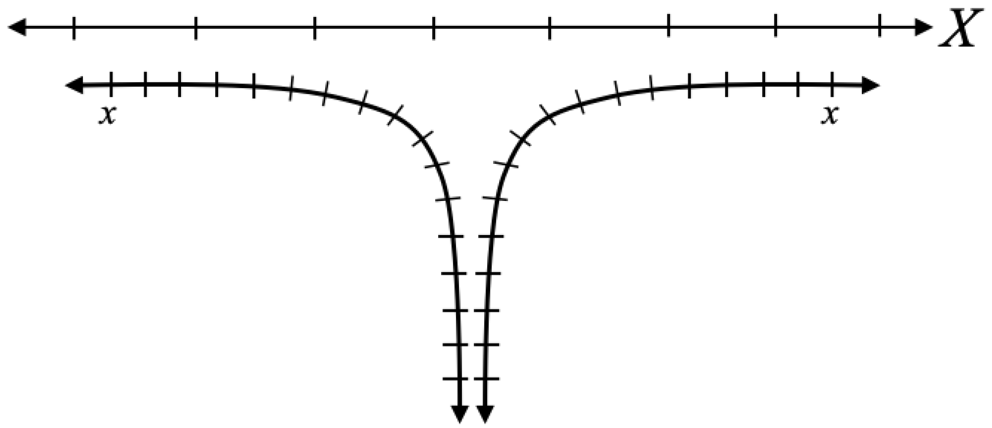
The important difference between the Schwarzschild and Kruskal-Szekeres coordinates is that at the horizon, all worldlines approach the the event horizon asymptotically in Schwarzschild coordinates, whereas, as we can see in Figure 6, the worldlines in Kruskal-Szekeres coordinates can approach the event horizon just like it approaches any other location. This lead to the belief that there is nothing special at the horizon and the problems with the Schwarzschild coordinates at the horizon are only the result of a coordinate singularity. But as we saw in Section 3, when taking a presentist perspective, all infalling worldlines actually intersect there and from the perspective of infalling observers, space contracts infinitely as the fallers approach the horizon. The discrepancy in the coordinate systems can be understood by acknowledging the extrinsic nature of the Kruskal-Szekeres coordinates and examining the analogy depicted in Figure 10 below:
In Figure 10, we see two lines depicting some space where each side of the space plunges downward infinitely so that the lines approach each other asymptotically. The lines don’t ever actually meet, they just get infinitesimally closer and closer to each other. The intrinsic coordinates are the x coordinates that follow the actual geometry. The x coordinate would therefore be analogous to the Schwarzschild coordinates. We also have an X coordinate, which is an extrinsic coordinate that is essentially laid on top of the geometry. We can clearly see in the figure that in the intrinsic x coordinate, the point directly between the two lines of the geometry is a special one. It is a discontinuity in the geometry separating the left and right lines of the geometry. But in the extrinsic X coordinate, there is nothing special there at all. With this coordinate, you can move from one side of the discontinuity to the other the same way you can move between any other two points, and so if you treated the X coordinate as being intrinsic, you would be led to believe that there is nothing special about the geometry at that point, even though we clearly see from Figure 10 that the midpoint physically separates the two halves of the geometry.
We have an analogous situation with the Kruskal-Szekeres coordinate chart. The intrinsic Schwarzschild coordinates are telling us the geometry is discontinuous there. We know this because the worldlines from either side of the horizon approach it asymptotically. But the fact that the curvature is finite at the horizon is also an indication that the internal and external spacetimes are separate. In Figure 10, if the lines approached each other asymptotically but actually connected, that connection would be infinitely sharp and therefore we would have infinite curvature there. But if they never connect and only approach each other asymptotically, then the curvature for each line will remain finite on approach to the separation point from either side. The Kruskal-Szekeres coordinates are giving us a coordinate system describing the geometry from the ’outside’ and just as in Figure 10, it obscures the asymptotic separation of the two regions, making it appear that the horizon is not a special place when it has been clearly demonstrated to be a point of separation between spacetimes. And even though the metric in Kruskal-Szekeres coordinates is regular at the horizon, it is also notable that the definitions of T and X need to be changed when going between regions (as demonstrated with equations 3 and 4), further supporting the fact that the horizon separates two different spacetimes.
The question then remains, what is region II of Figure 1 describing. We know that the Schwarzschild solution describes all spherically symmetric vacua. In region I, the t coordinate is spacelike while the r coordinate is timelike. We see that the the horizon, the spatial t coordinate density is infinite and the coordinate lines separate as one moves from the horizon to . As discussed in Section 2, the space of the metric at a given time is homogeneous and isotropic. It was also demonstrated in the case of the external solution that the source of the metric is at . It stands to reason then that the source of the internal solution is also at that point. So the internal solution describes a spherically symmetric vacuum surrounded by a horizon which, from the perspective of an observer at some r between the horizon and , surrounds the vacuum infinitely far away in space and at some finite time in the past. And from the perspective of that observer, this horizon, which looks like a surrounding sphere, is a time where space is infinitely dense. A spacetime fitting this description would be any empty space in the Universe whose surrounding mass is spherically symmetric. Voids in the cosmic web would be an example of such a spacetime, and the horizon of the metric in this case would be the Big Bang, which is an event at some finite time in the past that surrounds all points in the Universe which has an infinite density. And an observer in the present Universe can never reach the Big Bang, no matter how far they travel through space, which is in alignment with the fact that the surface, from the perspective of a present observer, is infinitely far away from them in space. So we might think of the expanding Universe as baking bread where the air pockets that expand as the bread bakes give the bread a web-like structure over time, where the bread itself would be analogous to the cosmic filaments of matter in the Universe. A full cosmological analysis of the internal solution will be completed in a followup work which will also discuss all four regions of the Kruskal-Szekeres coordinate chart as well as the curvature singularity at .
6. Conclusions
An analysis of the Schwarzschild metric described with Kruskal-Szekeres coordinates has revealed the following:
- A surface of constant r in the external region is described by a one-sheeted hyperboloid of revolution and a surface of constant r in the internal region is described by a two-sheeted hyperboloid of revolution.
- Examining the spacelike Killing vectors in the internal solution in Kruskal-Szekeres coordinates reveals that space in the internal metric at a given time is homogeneous and isotropic.
- The Schwarzschild metric is symmetric under spherical rotation as well as hyperbolic rotation. The hyperbolic rotation symmetry is what makes the external solution static and the internal solution homogeneous and isotropic at a given time.
- The hyperbolic symmetry allows us to create a ’presentist perspective’ of the external solution where the present point on the worldline is always at and past worldline points get hyperbolically rotated to increasingly negative t values as time passes.
- Applying the ’presentist perspective’ to particles in freefall demonstrates that all particles falling toward the horizon will be coincident at the horizon no matter where or when they begin falling relative to each other.
- It was proven that all worldlines approaching the event horizon become null as predicted by the presentist construction. This is because the r and t basis vectors are aligned with the X and T basis vectors when such that always has a clear physical meaning there, with the slope representing the fraction of the speed of light at which the particle is falling. This proves that the Schwarzschild radius does not represent a coordinate singularity, but is in fact the end point of gravitational collapse and the point on the Kruskal-Szekeres coordinate chart is the source of the gravitational field.
- In the frame of freefalling observers, the horizon becomes length contracted the closer the observer gets to the horizon, until it is infinitely contracted as they approach the horizon such that there is no space to fall into beyond the horizon. The source of the metric is therefore at the horizon, not at .
- The Kruskal-Szekeres coordinates are extrinsic coordinates in contrast to the Schwarzschild coordinates which are intrinsic. The extrinsic nature of the Kruskal-Szekeres coordinates obscures the true nature of the geometry at the horizon which is why the metric appears regular at the horizon in those extrinsic coordinates while the worldlines in the intrinsic Schwarzschild coordinates are asymptotic there.
- The internal and external regions of the metric are separate spacetimes separated by an asymptote at the horizon.
- The internal solution describes a spherically symmetric vacuum surrounded by an infinitely dense shell that is infinitely far away in space and exists at a finite time in the past.
- The internal solution is interpreted as any spherically symmetric vacuum in the Universe surrounded by mass, such as the cosmic voids between the cosmic filaments. Under this interpretation, the event horizon of the internal solution would be the Big Bang of the Universe
- Further rigorous investigation into the cosmological nature of the internal solution will be completed in a followup work.
Data Availability Statement
All data generated or analysed during this study are included in this published article [and its supplementary information files].
Conflicts of Interest
There are no competing interests
References
- Carroll, S.M. Lecture Notes on General Relativity, 1997, [arXiv:gr-qc/9712019v1].
- Figures 1, 6, 7, and 8 are modifications of: ’Kruskal diagram of Schwarzschild chart’ by Dr Greg. Licensed under CC BY-SA 3.0 via Wikimedia Commons. http://commons.wikimedia.org/wiki/File:Kruskal_diagram_of_Schwarzschild_chart.svg#/media/File:Kruskal_diagram_of_Schwarzschild_chart.svg, Accessed in 2017.
- Augousti, A.; Gawełczyk, M.; Siwek, A.; Radosz, A. Touching ghosts: Observing free fall from an infalling frame of reference into a Schwarzschild black hole. European Journal of Physics - EUR J PHYS 2012, 33, 1–11. [Google Scholar] [CrossRef]
- Raine, D.; Thomas, E. Black Holes a Student Text; Imperial College Press, 2015.
Figure 1.
Kruskal-Szekeres Coordinate Chart
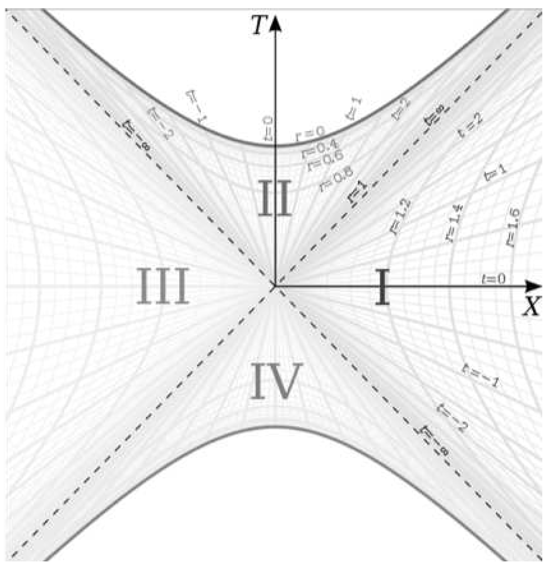
Figure 2.
2D Surfaces of Constant r for Internal and External Metrics
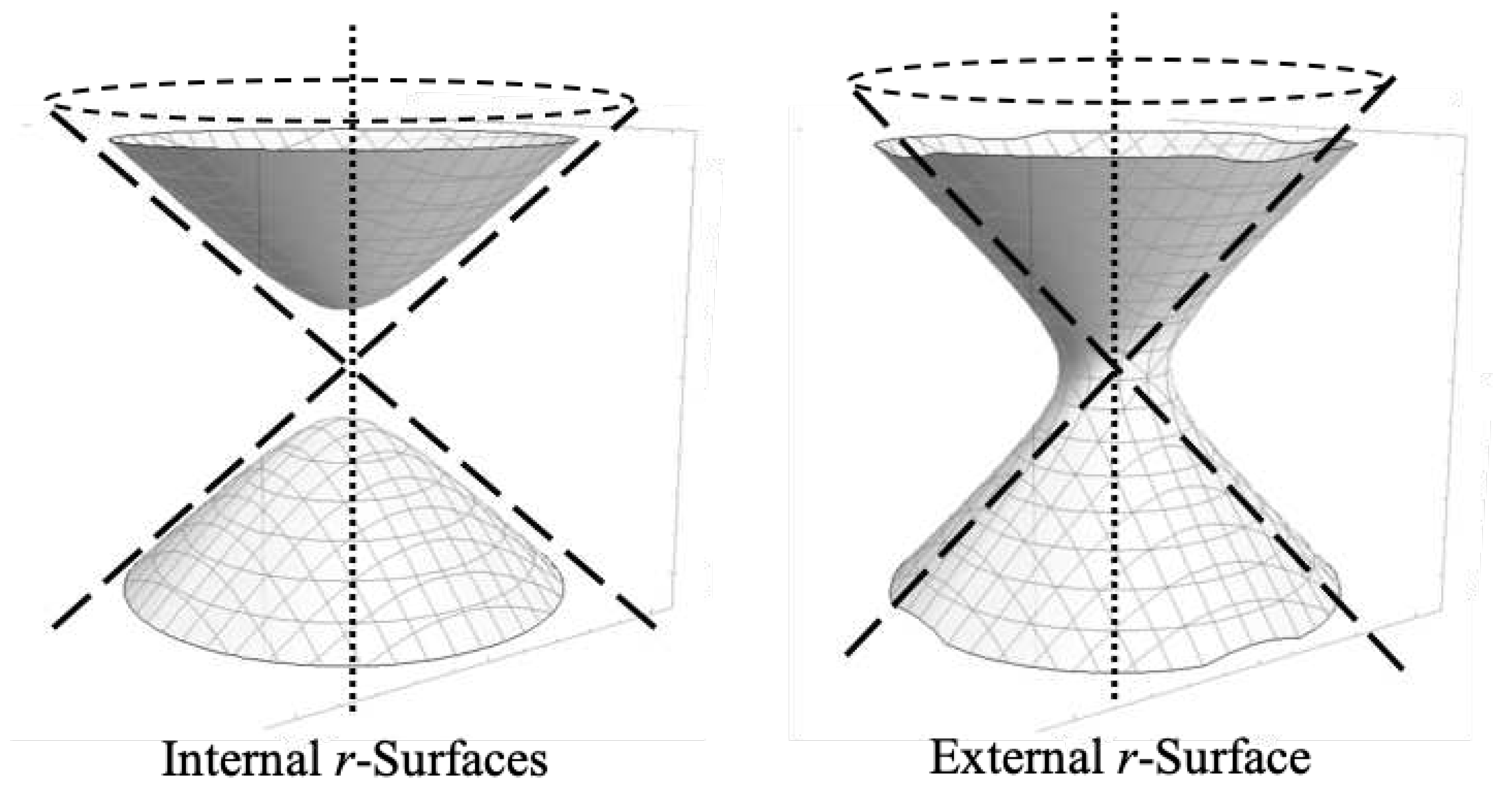
Figure 3.
Radial Killing/Basis Vectors on a Surface of Constant r
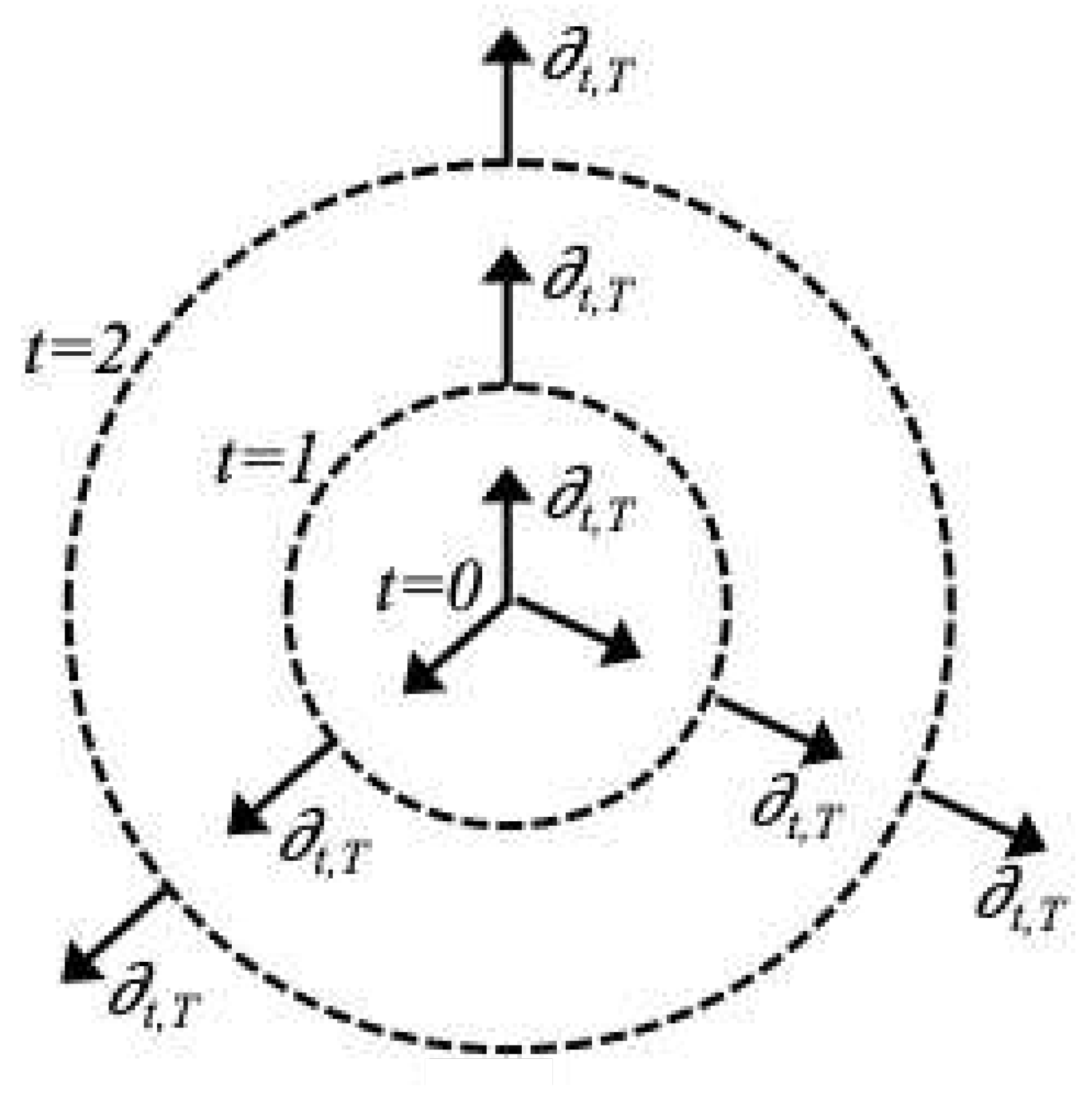
Figure 4.
Cartesian Killing/Basis Vectors on a Surface of Constant r
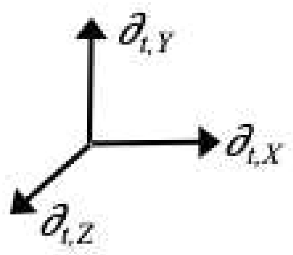
Figure 5.
Worldline of a Particle for One Revolution of Circular Orbit
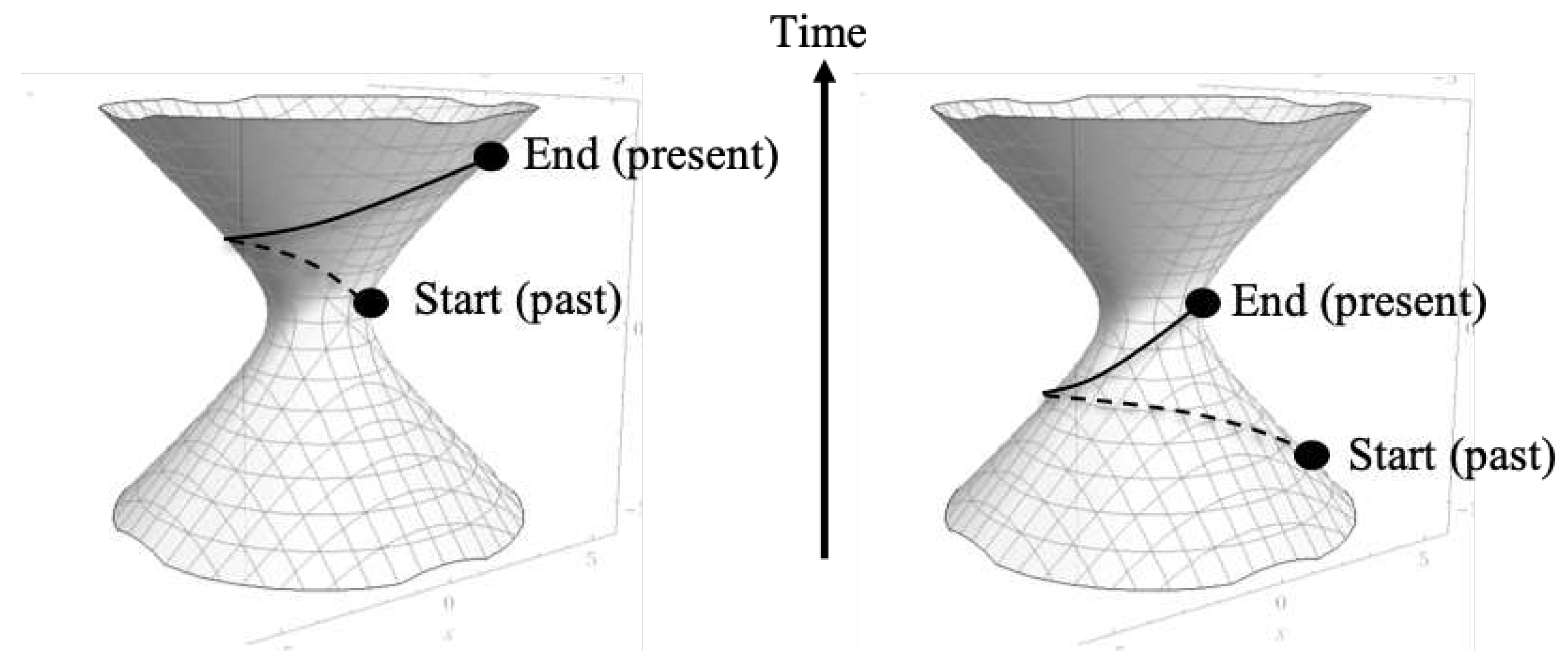
Figure 6.
Worldlines of Two Particles in Radial Freefall
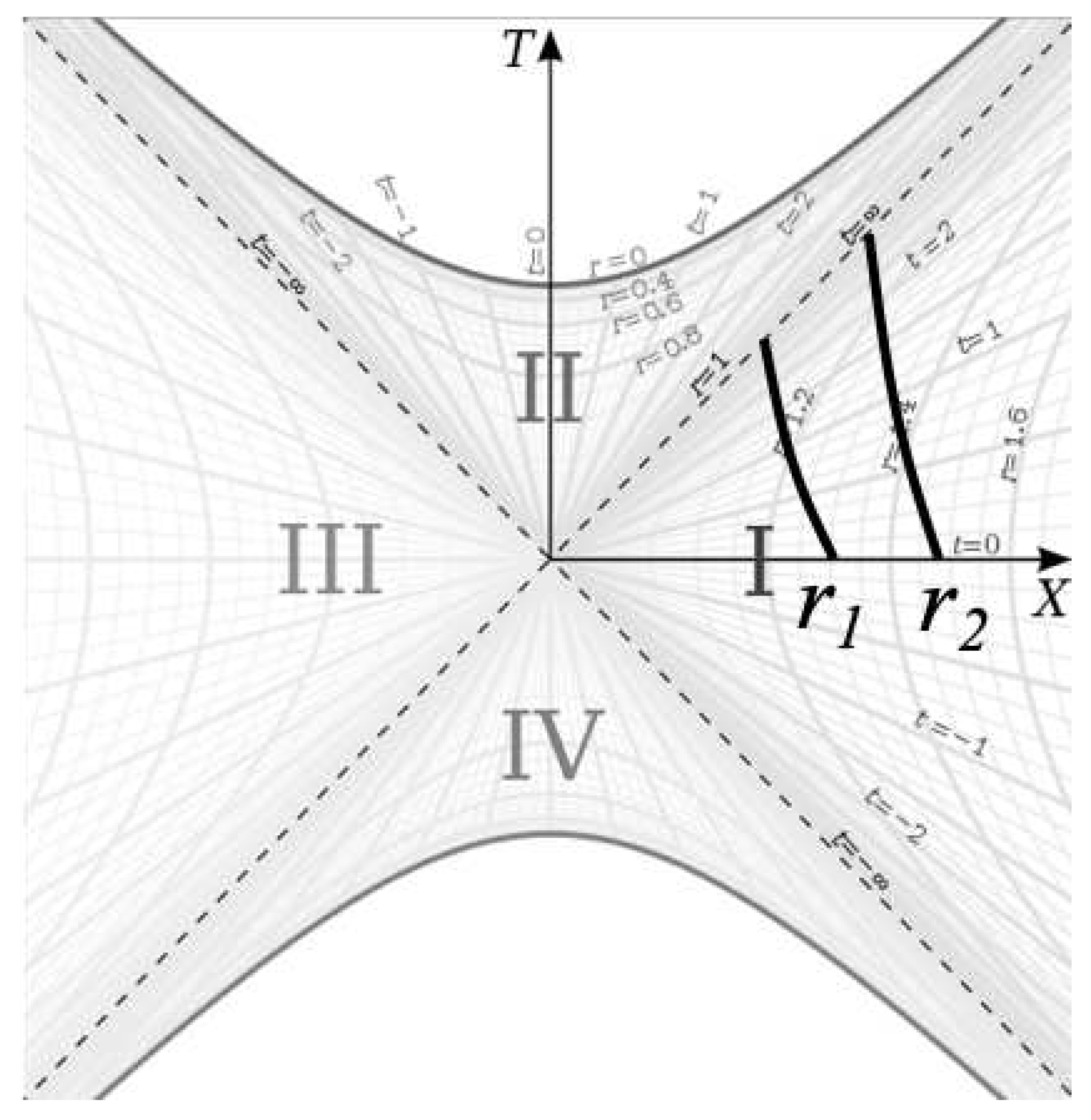
Figure 7.
Worldlines of Two Particles in Radial Freefall - Presentist Perspective
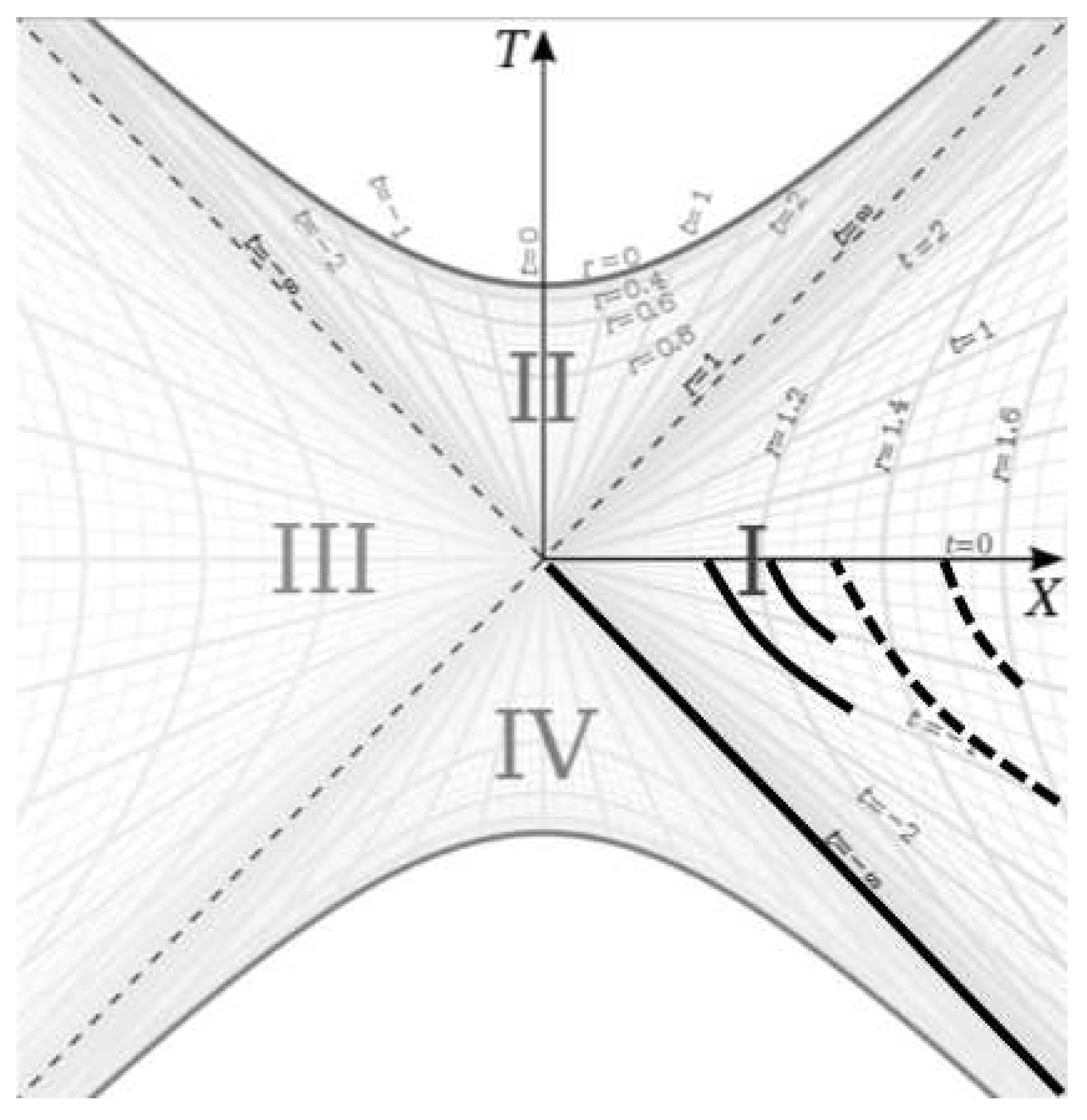
Figure 8.
Lorentz Boosted Frames During Freefall
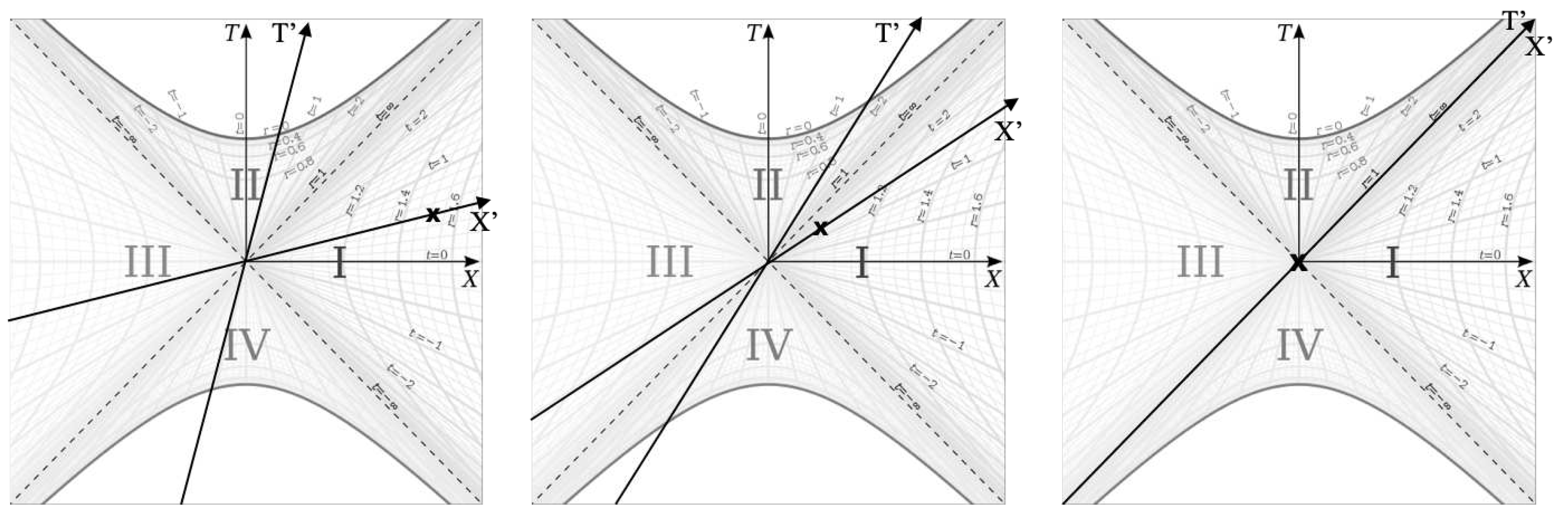
Figure 9.
Scout and Jem on a Collapsing Shell
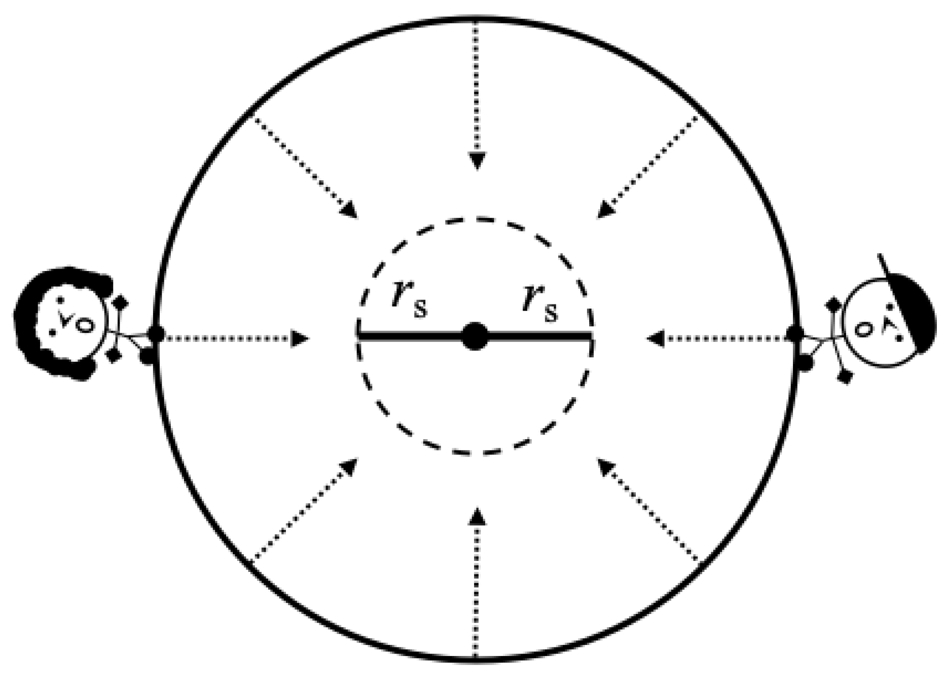
Figure 10.
Extrinsic vs. Intrinsic Coordinates
Disclaimer/Publisher’s Note: The statements, opinions and data contained in all publications are solely those of the individual author(s) and contributor(s) and not of MDPI and/or the editor(s). MDPI and/or the editor(s) disclaim responsibility for any injury to people or property resulting from any ideas, methods, instructions or products referred to in the content. |
© 2023 by the authors. Licensee MDPI, Basel, Switzerland. This article is an open access article distributed under the terms and conditions of the Creative Commons Attribution (CC BY) license (http://creativecommons.org/licenses/by/4.0/).
Copyright: This open access article is published under a Creative Commons CC BY 4.0 license, which permit the free download, distribution, and reuse, provided that the author and preprint are cited in any reuse.


