Submitted:
17 January 2023
Posted:
18 January 2023
You are already at the latest version
Abstract
The standard Cosmological model (LCDM) assumes that the expanding spacetime around us is infinite, which is inconsistent with the observed cosmic acceleration unless we include Dark Energy (DE) or a Cosmological Constant ($\Lambda$). But the observed cosmic expansion can also be explained with a finite mass $M$, inside a uniform expanding sphere, with empty space outside. An object with mass $M$ has a gravitation radius $r_S=2GM$. When $M$ is all contained within $r_S$, this is a Black Hole (BH). Nothing can escape from $r_S$, which becomes a boundary for the inside dynamics. In the limit where there is nothing outside, the inside corresponds to a local isolated Universe. The $r_S$ boundary condition corresponds to an effective force which is mathematically equivalent to $\Lambda=3/r_S^2$. We can therefore interpret cosmic acceleration as a measurement of the gravitational boundary of our Universe, with a mass $M = \frac{c^2}{2G}\sqrt{3/\Lambda} \simeq 6 \times 10^{22} M_{\odot}$. Such BH Universe (BHU) is observationally very similar to the LCDM, except for the very large scale perturbations, which are bounded by $r_S$.
Keywords:
Cosmology
; Dark Energy
; General Relativity
; Black Holes
1. Introduction
The standard cosmological model ([1,2]), also called LCDM, assumes that our Universe correspond to a global space-time that began in a hot Big Bang (BB) expansion at the very beginning time. Such initial conditions seem to violate the classical concept of energy conservation and are very unlikely ([3,4,5,6]). According to this singular start BB model, the full observable Universe came out of (macroscopic) nothing, resulting from some Quantum Gravity vacuum fluctuations that we can only speculate about. We will never be able to test experimentally these ideas because of the enormous energies involved () and here is no direct evidence that this ever occurred. The BB model also requires three more exotic patches: Cosmic Inflation, Dark Matter and Dark Energy (DE), for which we have no direct evidence or understanding at any fundamental level.
Despite these shortfalls, the LCDM model seems very successful in explaining most observations by fitting just a handful of free cosmological parameters. Here we how how the Black Hole Universe (BHU) can be an alternative paradigm to the LCDM and elaborate that the main difference between these two approaches reside in whether the mass-energy of our Universe is finite or not.
The fact that the universe might be generated from the inside of a BH has been studied extensively in the literature. [7] and [8] proposed that the FLRW metric could be the interior of a BH. But these early proposals were not proper GR solutions, but just incomplete analogies (see [9]). [10] presented a more rigorous demonstration within classical GR that that the FLRW metric could be inside a BH, something that was also clear from the works of [11]. Many of the previous approaches ([12,13,14,15,16,17,18]) involve modifications to Classical GR. There are also some simple scalar field examples (e.g. [14]) which presented models within the scope of a classical GR and classical field theory with a false vacuum interior. A particular case are Bubble or Baby Universe solutions where the BH interior is de-Sitter metric ([19,20,21,22,23,24,25,26]). In the BHU solution ([27,28,29,30]) and also in the previously cite works of [11] and [10], no surface terms (or Bubble) are needed and the inside is not filled with a false vacuum, but with regular matter and radiation. The difference between the recent BHU and the earlier FLRW metric solutions inside a BH is the role of the term as a boundary condition ([29]). The model by [31] has the same name and similar features as the BHU, but the model is proposed as a new postulate to GR and not as a classical solution.
Here, we will start by reviewing in §Section 2 the classical GR solutions to the problem of a uniform spherical ball with fixed mass. In §Section 3 we will interpret what we mean by a fixed mass and we will then focus in §Section 4 on the corresponding BH solutions to show that the observed cosmic expansion is consistent with the BHU idea. We end with some conclusion and discussion of how the BHU form in §Section 5.
2. A uniform spherical ball of fixed mass
The most general metric with spherical symmetry in spherical coordinates and proper time has the form ([11,32,33]):
where we use units of speed of light and the radial coordinate will be taken here to be comoving with the matter content. This metric is sometimes called the Lemaitre-Tolman metric ([32,34]) or the Lemaitre-Tolman-Bondi (LTB) metric. This is a metric localized around a reference central point in space which we have set to be the origin () for simplicity.
For an observer moving with a perfect fluid the energy-momentum tensor is diagonal: , where is the energy density and is the pressure. The off-diagonal terms of the field equation are zero, e.g.: , which translates into:
This equation can be solved as: , where . The case corresponds a flat geometry:
so that there is only one function we need to solve: which corresponds to the radial proper distance. The field equations for r (with ) are:
where the dot here is . When is uniform, we have and , so that Eq.3 reproduces the flat (global) FLRW metric and Eq.4 is the corresponding solution: , which corresponds to a global solution (any point can be choosen as to be the center of the metric ). The non flat case can also be reproduced if we consider the more general case .
But the solution in Eq.4- can also be used to solve non-homogeneous cases. The simplest is the case of an expanding (or collapsing) uniform spherical ball inside a comoving coordinate and empty outside:
which reproduces the exact same FLRW metric and solution with the same mass inside as in the infinite FLRW case:
where . The only difference is that this is now a local solution with empty space outside . The Hubble-Lemaitre expansion law: of Eq.4 with is the same for the global or the local FLRW solution inside . This is a consequence of Birkhoff’s theorem (see [35,36]), since a sphere cut out of an infinite uniform distribution has the same spherical symmetry. Thus, the FLRW metric is both a solution to a global homogeneous (i.e. infinite M) uniform background and also to the inside of a local (finite mass) uniform sphere centered around one particular point. The local solution is called the FLRW cloud ([29]).
3. Relativistic mass
The Misner and Sharp ([33]) mass-energy inside a spatial hypersurface of Eq.1, given by , is:
where is the 3D spatial volume element of the metric in (we recover here units if to check the non relativistic limit). The first term is the material or passive mass (which we call here M):
and corresponds to Eq.. We can then interpret the next two terms in Eq.8 as the contribution to mass energy from the kinetic and potential energy (see also [37] for a more general description). In the non relativistic limit () these two terms are negligible and . But in general, as indicated by Eq.8, can not be expressed as a sum of individual energies as also appears inside the integral, reflecting the non-linear nature of gravity. But in the case of Eq.4, the kinetic and potential energy terms cancel for and we can interpret M as the total mass-energy of the system.
For the case in Eq.4-, the mass inside is constant for matter dominated fluid when . But in the early stages of the expansion, when the Energy-density is dominated by radiation or a fluid with a different equation of state the mass inside is a function . If we want M to be constant throughout its evolution we need the junction to be a function of time . In the case of mass-energy dominated by inside (and empty outside) we have and from Eq.:
where corresponds to radiation and to matter domination. So we need to find a physical solution with fixed mass M. More generally, for a fluid with several components :
we have
Thus, a solution with constant M requires:
Note that both R and here are just radial coordinates and not proper distances between events.
4. Black Hole solution
For the local top-hat distribution of Eq.6, if all the mass M is contained within the solution correspond to a Black Hole (BH, see [38]). In the limit where the exterior is empty, the gravitational radius should be interpreted as a boundary that separates the interior () from the exterior manifold. This creates and isolated Universe inside with a boundary condition at . As detailed in [28,29], starting from the general case with , the corresponding GHY boundary term ([39,40,41]) to the Einstein-Hilbert action requieres an effective term: , which changes the field equations Eq.4 into:
where in the last step we have use and M given by Eq.12. Note that Eq. does not change and we still have . The boundary adds another contribution to in Eq.8:
which also cancels out with the new Hubble law in Eq.14. In terms of , where :
where typically we have with for matter and for radiation. This is exactly what we measure in cosmological surveys. It shows how we can interpret the observed cosmic expansion as being a local BH solution, the BHU (instead of a global LCDM model with or DE). If there is also dark energy (DE) we have to add an additional term:
where is the DE equation of state. Given that the last 2 terms are approximately constant (for ) there is no way to distinguish them using measurements of the Hubble-Lemaitre law. Current observations tell us that indeed ([42]) and the sum of the 2 terms is an effective term such that or, in other words:
If , we have that and the mass of our Universe is:
where we have returned to units of here to be more explicit. This corresponds to the BHU. In the other limit, if we recover the infinite LCDM model with and . Both models have a future Event Horizon (E.H.) R::
which is bounded by ([29]): anything that is at is outside causal reach. Here is the maximum proper distance that a photon can travel. Fig.Figure 1 shows a comparison of the two possible interpretations.
We could also have an intermediate situation, but it would be quite unnatural that (from M) and (from DE) are fine tuned to both contribute to the observed cosmic acceleration. We therefore have to choose one of the two interpretations. Given that is a non physical (and not causally possible) solution and that we do not know what DE is, it seems more plausible and simpler to interpret cosmic acceleration as a measurement for the mass M of our Universe. In this case and the raw value of is also . Our Universe is therefore inside a local BHU.
5. Conclusion
We have interpreted the observed to be an effective term that corresponds to the gravitational radius of our local Universe. This has several implications:
- Our Universe is a local solution inside its gravitational radius . It is therefore a Black Hole Universe (BHU).
- The dynamical time associated to M in our Universe is , which is close to the measured age of the oldest galaxies and stars that we observe.
- An observer placed anywhere within the local BHU measures the same background as one within the LCDM ([29]).
- Our BHU might not be unique: there could also exist other Universes, like ours, elsewhere. This is part of the The Copernican Revolution: our place is not special.
How did such a BHU form? Here we enter the more speculative grounds of the Big Bang theories. The BHU could have formed in a similar way as the standard LCDM universe: out of one of the many existing models of Cosmic Inflation ([46,47,48,49,50]) or from some of the Quantum Gravity alternatives (e.g. [6,13,16,51,52]).
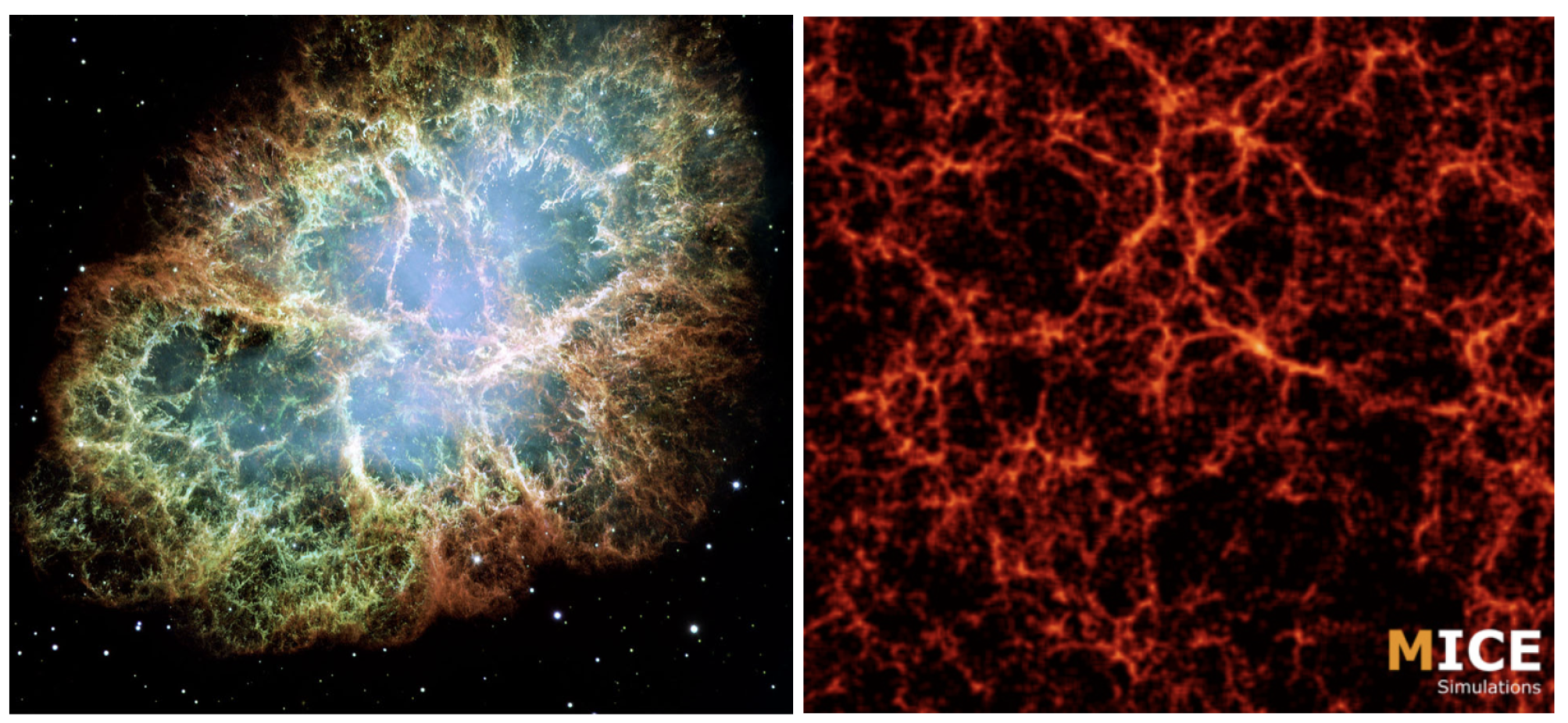
The BHU could have also formed in a much simpler way, just like the first stars: collapsing and exploding in a Supernova following the known laws of Physics ([30]). Left panel of Figure 2 shows the Crab Nebula, a remnant of a Supernova, which can be thought as a small version of our Universe today. In such case, Cosmic Inflation or Quantum Gravity explanations are not needed to understand the origin of our cosmic expansion. Such beginning would provide us with an anthropic explanation for the observed value of and the coincidence problem. It also yields new candidates for Dark Matter in the form of compact remnants of the collapse and bouncing phases, such as primordial BHs and primordial Neutron Stars ([30]).
The BHU exists within a larger background that may or may not be totally empty outside. In the later case, will increase if there is accretion from outside. This case is more speculative and needs to be studied in more detail, but it would result in an effective term that decreases with time (). The alternative interpretation is that M (and therefore ) are infinite so that the measured can only be attributed to DE. This is the standard (LCDM) interpretation. In our view, this alternative is less appealing because it involves non physical infinite, non causal structure ([53,54]) and new components, DE or , which are not really needed.
Data Availability Statement
No new data is presented in this paper.
Acknowledgments
We acknowledge grants from Spain (PGC2018-102021-B-100, CEX2020-001058-M) and the EU (LACEGAL 734374).
References
- Dodelson, S. Modern cosmology, Academic Press, NY; 2003.
- Weinberg, S. Cosmology, Oxford University Press; 2008.
- Tolman, R.C. On the Problem of the Entropy of the Universe as a Whole. Physical Review 1931, 37, 1639–1660. [Google Scholar] [CrossRef]
- Dyson, L.; Kleban, M.; Susskind, L. Disturbing Implications of a Cosmological Constant. J.of High Energy Phy 2002, 2002, 011. [Google Scholar] [CrossRef]
- Penrose, R. Before the big bang: An outrageous new perspective and its implications for particle physics. Conf. Proc. C 2006, 060626, 2759–2767. [Google Scholar]
- Brandenberger, R. Initial conditions for inflation — A short review. Int. Journal of Modern Physics D 2017, arXiv:hep-th/1601.01918]26, 1740002–126. [Google Scholar] [CrossRef]
- Pathria, R.K. The Universe as a Black Hole. Nature 1972, 240, 298–299. [Google Scholar] [CrossRef]
- Good, I.J. Chinese universes. Physics Today 1972, 25, 15. [Google Scholar] [CrossRef]
- Knutsen, H. The idea of the universe as a black hole revisited. Gravitation and Cosmology 2009, 15, 273–277. [Google Scholar] [CrossRef]
- Stuckey, W.M. The observable universe inside a black hole. American Journal of Physics 1994, 62, 788–795. [Google Scholar] [CrossRef]
- Oppenheimer, J.R.; Snyder, H. On Continued Gravitational Contraction. Physical Review 1939, 56, 455–459. [Google Scholar] [CrossRef]
- Smolin, L. Did the Universe evolve? Classical and Quantum Gravity 1992, 9, 173–191. [Google Scholar] [CrossRef]
- Easson, D.A.; Brandenberger, R.H. Universe generation from black hole interiors. J. of High Energy Phy. 2001, 2001, 024. [Google Scholar] [CrossRef]
- Daghigh, R.G.; Kapusta, J.I.; Hosotani, Y. False Vacuum Black Holes and Universes. arXiv:gr-qc/0008006, 2000. [Google Scholar]
- Firouzjahi, H. Primordial Universe Inside the Black Hole and Inflation. arXiv e-prints 2016, arXiv:1610.03767. [Google Scholar]
- Popławski, N. Universe in a Black Hole in Einstein-Cartan Gravity. ApJ 2016, arXiv:gr-qc/1410.3881]832, 96. [Google Scholar] [CrossRef]
- Oshita, N.; Yokoyama, J. Creation of an inflationary universe out of a black hole. Physics Letters B 2018, 785, 197–200. [Google Scholar] [CrossRef]
- Dymnikova, I. Universes Inside a Black Hole with the de Sitter Interior. Universe 2019, 5, 111. [Google Scholar] [CrossRef]
- Gonzalez-Diaz, P.F. The space-time metric inside a black hole. Nuovo Cimento Lettere 1981, 32, 161–163. [Google Scholar] [CrossRef]
- Grøn. ; Soleng, H.H. Dynamical instability of the González-Díaz black hole model. Physics Letters A 1989, 138, 89–94. [Google Scholar] [CrossRef]
- Blau, S.K.; Guendelman, E.I.; Guth, A.H. Dynamics of false-vacuum bubbles. PRD 1987, 35, 1747–1766. [Google Scholar] [CrossRef] [PubMed]
- Frolov, V.P.; Markov, M.A.; Mukhanov, V.F. Through a black hole into a new universe? Phys Let B 1989, 216, 272–276. [Google Scholar] [CrossRef]
- Aguirre, A.; Johnson, M.C. Dynamics and instability of false vacuum bubbles. PRD 2005, 72, 103525. [Google Scholar] [CrossRef]
- Mazur, P.O.; Mottola, E. Surface tension and negative pressure interior of a non-singular `black hole’. Classical and Quantum Gravity 2015, 32, 215024. [Google Scholar] [CrossRef]
- Garriga, J.; Vilenkin, A.; Zhang, J. Black holes and the multiverse. JCAP 2016, arXiv:hep-th/1512.01819]2016, 064. [Google Scholar] [CrossRef]
- Kusenko, A.e. Exploring Primordial Black Holes from the Multiverse with Optical Telescopes. PRL 2020, arXiv:astro-ph.CO/2001.09160]125, 181304. [Google Scholar] [CrossRef] [PubMed]
- Gaztañaga, E. How the Big Bang Ends Up Inside a Black Hole. Universe 2022, 8, 257. [Google Scholar] [CrossRef]
- Gaztañaga, E. The Cosmological Constant as Event Horizon. Symmetry 2022, 14, 300–2202. [Google Scholar] [CrossRef]
- Gaztañaga, E. The Black Hole Universe, part I. Symmetry 2022, 14, 1849. [Google Scholar] [CrossRef]
- Gaztañaga, E. The Black Hole Universe, part II. Symmetry 2022, 14, 1984. [Google Scholar] [CrossRef]
- Zhang, T.X. The Principles and Laws of Black Hole Universe. Journal of Modern Physics 2018, 9, 1838–1865. [Google Scholar] [CrossRef]
- Tolman, R.C. Effect of Inhomogeneity on Cosmological Models. Proc. of the Nat. Academy of Science 1934, 20, 169–176. [Google Scholar] [CrossRef]
- Misner, C.W.; Sharp, D.H. Relativistic Equations for Adiabatic, Spherically Symmetric Gravitational Collapse. Physical Review 1964, 136, 571. [Google Scholar] [CrossRef]
- Lemaître, G. Un Univers homogène de masse constante et de rayon croissant rendant compte de la vitesse radiale des nébuleuses extra-galactiques. Annales de la S.S. de Bruxelles 1927, 47, 49–59. [Google Scholar]
- Johansen, N.; Ravndal, F. On the discovery of Birkhoff’s theorem. General Relativity and Gravitation 2006, 38, 537–540. [Google Scholar] [CrossRef]
- Faraoni, V.; Atieh, F. Turning a Newtonian analogy for FLRW cosmology into a relativistic problem. PRD 2020, 102, 044020. [Google Scholar] [CrossRef]
- Hayward, S.A. Gravitational energy in spherical symmetry. Phys. Rev. D 1996, 53, 1938–1949. [Google Scholar] [CrossRef] [PubMed]
- Firouzjaee, J.T.; Mansouri, R. Asymptotically FRW black holes. Gen. Rel. Grav. 2010, arXiv:astro-ph/0812.5108]42, 2431–2452. [Google Scholar] [CrossRef]
- York, J.W. Role of Conformal Three-Geometry in the Dynamics of Gravitation. PRL 1972, 28, 1082–1085. [Google Scholar] [CrossRef]
- Gibbons, G.W.; Hawking, S.W. Cosmological event horizons, thermodynamics, and particle creation. PRD 1977, 15, 2738–2751. [Google Scholar] [CrossRef]
- Hawking, S.W.; Horowitz, G.T. The gravitational Hamiltonian, action, entropy and surface terms. Class Quantum Gravity 1996, 13, 1487. [Google Scholar] [CrossRef]
- DES Collaboration. Cosmological Constraints from Multiple Probes in the Dark Energy Survey. PRL 2019, arXiv:astro-ph.CO/1811.02375]122, 171301. [Google Scholar] [CrossRef]
- Fosalba, P.; Gaztañaga, E. Explaining cosmological anisotropy: evidence for causal horizons from CMB data. MNRAS 2021, 504, 5840–5862. [Google Scholar] [CrossRef]
- Gaztañaga, E.; Camacho-Quevedo, B. What moves the heavens above? Physics Letters B 2022, arXiv:astro-ph.CO/2204.10728]835, 137468. [Google Scholar] [CrossRef]
- Carretero, J.; Castander, F.J.; Gaztañaga, E.; Crocce, M.; Fosalba, P. An algorithm to build mock galaxy catalogues using MICE simulations. MNRAS 2015, 447, 646–670. [Google Scholar] [CrossRef]
- Starobinskiǐ, A.A. Spectrum of relict gravitational radiation and the early state of the universe. Soviet J. of Exp. and Th. Physics Letters 1979, 30, 682. [Google Scholar]
- Guth, A.H. Inflationary universe: A possible solution to the horizon and flatness problems. PRD 1981, 23, 347–356. [Google Scholar] [CrossRef]
- Linde, A.D. A new inflationary universe scenario. Physics Letters B 1982, 108, 389–393. [Google Scholar] [CrossRef]
- Albrecht, A.; Steinhardt, P.J. Cosmology for Grand Unified Theories with Radiatively Induced Symmetry Breaking. PRL 1982, 48, 1220–1223. [Google Scholar] [CrossRef]
- Liddle, A.R. Observational tests of inflation. arXiv e-prints 1999, arXiv:astro-ph/astro-ph/9910110. [Google Scholar]
- Novello, M.; Bergliaffa, S.E.P. Bouncing cosmologies. Phys.Rep 2008, 463, 127–213. [Google Scholar] [CrossRef]
- Ijjas, A.; Steinhardt, P.J. Bouncing cosmology made simple. Classical and Quantum Gravity 2018, 35, 135004. [Google Scholar] [CrossRef]
- Gaztañaga, E. The size of our causal Universe. MNRAS 2020, 494, 2766–2772. [Google Scholar] [CrossRef]
- Gaztañaga, E. The cosmological constant as a zero action boundary. MNRAS 2021, 502, 436–444. [Google Scholar] [CrossRef]
Figure 1.
TOP PANELS: Comparison of the proper radius of the BHU (left) and the LCDM (right) models. The blue circle represents a sphere of radius . The red one corresponds to the future event horizon R of the FLRW metric inside. Both and R expand towards the fixed black sphere: the gravitational radius in the BHU and in LCDM. Scales are not causally connected, despite this, the LCDM has the same density everywhere. BOTTOM PANELS: evolution of the the different radius as a function of time (given by the scale factor a) for . The dashed green line is the past light-cone or observable Universe: . We can only see photons emitted in the past along this green line radial trajectory (in all directions).
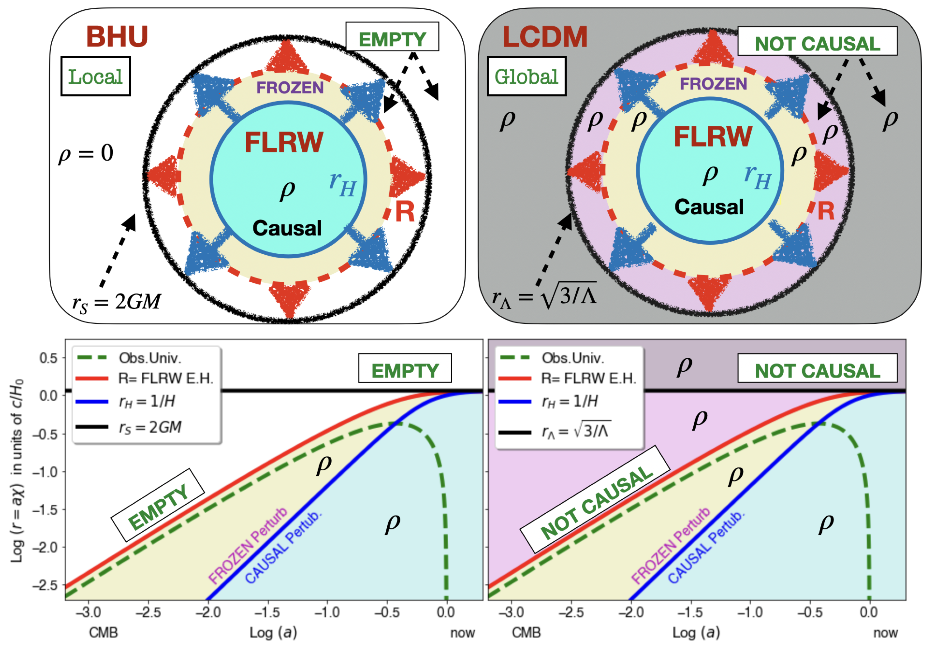
Figure 2.
LEFT: The expanding Crab Nebula Supernova remnant, as observed in 1999 from the Hubble Space Telescope, 945 years after the explosion. The observed pulsar remnant could be part of the Dark Matter, in the form of primordial Neutron Stars and primordial BHs. RIGHT: the MICE simulation ([45]) of large scale structures in our expanding Universe.
Disclaimer/Publisher’s Note: The statements, opinions and data contained in all publications are solely those of the individual author(s) and contributor(s) and not of MDPI and/or the editor(s). MDPI and/or the editor(s) disclaim responsibility for any injury to people or property resulting from any ideas, methods, instructions or products referred to in the content. |
© 2023 by the authors. Licensee MDPI, Basel, Switzerland. This article is an open access article distributed under the terms and conditions of the Creative Commons Attribution (CC BY) license (http://creativecommons.org/licenses/by/4.0/).
Copyright: This open access article is published under a Creative Commons CC BY 4.0 license, which permit the free download, distribution, and reuse, provided that the author and preprint are cited in any reuse.


