Cosmology at the End of Time

1. Introduction

The concordance $\Lambda$CDM model provides a compelling description of the Universe from superhorizon scales all the way down to supercluster scales with only a few free parameters, essentially the energy density of ordinary (`baryonic’) matter, cold dark matter (CDM) and dark energy (DE), along with the free parameters describing the amplitude and tilt of primordial matter power spectrum, as well as the optical depth to Compton scattering at reionization that took place at $z\sim 6$. The model is consistent with a broad spectrum of cosmological observations, e.g. the cosmic microwave background (CMB) anisotropy and polarization measurements, Type Ia supernovae (SNIa), baryonic oscillation (BAO), galaxy correlation and shear maps, etc. However, $\Lambda$CDM is still plagued by a few long-standing puzzles.

The largest contribution to the present-day cosmic energy budget is made by the vacuum-like DE component. Heuristic quantum field theoretic arguments imply that the vacuum energy density is $O\left(1\right)M_p^4$, e.g. [1], where $M_p$ is the Planck mass, and the typical lifetime of a Universe dominated by such energy density is typically the Planck time. For decades it has been hoped that the vacuum energy density identically vanishes by virtue of some yet-to-be-discovered symmetry principle. In 1998 SNIa measurements revealed that not only that the vacuum energy density does not vanish, nearly $69\%$ of the cosmic energy budget at present is accounted for by a cosmological constant, $\Lambda$, that effectively contributed a vacuum-like energy density $\sim 122$ orders of magnitude smaller than $O\left(1\right)M_p^4$. Recently, it has been claimed by the Dark Energy Spectroscopic Instrument (DESI) team based on [2,3] observations that the DE equation of state (EOS) evolves, implying that DE is not vacuum-like and is more likely to be described by a dynamical scalar field, which is foreign to the standard model (SM) of particle physics.

The fact that the present-day energy budget consists of $69\%$ of DE and the remaining $31\%$ contribution is accounted for by NR matter points towards a second problem associated with the cosmological constant in particular (and DE in general) – the `why now?’ problem. The observational fact that NR and vacuum-like energy contribute comparably at present to the cosmic energy budget in spite of their very different evolution histories implies that we live in a special era along the cosmic timeline. Specifically the NR to DE energy (assuming the latter is constant) ratio scales $\propto {(1+z)}^{-3}$, and for it to be of order unity at present it must have been fine-tuned at, e.g. 81 decimal places at the grand unified theory (GUT) energy scale. For reference, the global spatial curvature of the Universe must have been fine-tuned at that era at merely 27 decimal places for the Universe to be nearly flat at present. The latter fine-tuning was a major motivation for proposing an inflationary phase at the very early Universe. Tracking models, e.g. [4,5,6,7,8], CDM-DE interaction [9,10,11,12,13,14] as well as other explanations, e.g. [15,16,17,18,19,20,21,22,23,24,25,26,27,28,29,30,31,32,33,34,35,36] have been proposed as remedies for the apparent Cosmic Coincidence. Anthropic considerations received considerable weight as well, e.g. [1,37,38,39,40,41,42,43,44,45,46,47,48,49,50,51,52,53]. Notably, and not unrelated to this apparent coincidence, the very existence of DE could not have been inferred from observations if either ${\rho }_{DE}\ll {\rho }_m$ or ${\rho }_m\ll {\rho }_{DE}$, e.g. [54].

Motivated by certain properties of `eternal inflation’ (the currently prevailing inflationary scenario) it has been suggested that cosmic time has an end, not only a beginning [55], with a significant likelihood that time will end in the next five billion years. Likewise, certain plausibility requirements from the model suggest that it decays in less that Gyrs [56]. On completely different grounds, it is shown here with a plausible toy model that by simply starting from a homogeneous and isotropic Universe with a non-standard time coordinate that is past- and future-unbounded a simple coordinate transformation leads to exactly the standard Friedmann-Robertson-Walker (FRW) model but with the usual cosmic time (as well and conformal time) coordinate that has an end much like it has a beginning. This, by itself, imposes a severe global constraint on the relative contributions of the various species to the cosmic energy budget, and addresses the `why now?’ problem by the realization that we are likely to be observing the Universe at its terminal point. In other words, rather than being atypical fortunate observers we are typical observers that are bound to observe the Universe with (theoretically) inferred fractional density parameters (with respect to the critical density) tantalizingly similar to those of the concordance $\Lambda$CDM model. Implications for the future of life in the Universe, and other considerations for future observations, e.g. [57,58,59,60,61,62,63,64,65,66,67,68,69,70,71,72,73,74,75] are of not much relevance if now is indeed the end of time (EOT). Likewise, introducing this modification to the $\Lambda$CDM model has bearing on certain aspects of the Cosmological Arrow of Time, the existence of Boltzmann Brains (BB’s) and other Freak Observers (FO’s), certain aspects of the feasibility of time travel, the black hole Information Paradox and the Simulation Hypothesis. All these are discussed below.

The paper is organized as follows. In Section 2 the standard cosmological model is described. In Section 3, we discuss a few possible ramifications of the possibility that the present time is the EOT in an otherwise concordance $\Lambda$CDM model. In Section 4 we construct the proposed cosmological model which is $\Lambda$CDM with a terminal cosmic time at the present. In Section 5 we argue that it is statistically very likely (under certain plausible assumptions) that we are located at the EOT. Section 6 demonstrates how the Cosmological Coincidence Problem (CCP) is naturally addressed in the proposed model. We summarize in Section 7.

Throughout, we adopt natural units where the Boltzmann constant, $k_B$, Planck constant, ℏ, and the speed of light, c, are all set to unity.

2. The FRW Spacetime

The most general homogeneous and isotropic space is described by the FRW spacetime

$$\begin{array}{c}\hfill d{s}^2=-d{t}^2+a^2\left(t\right)\left[{\displaystyle \frac{d{r}^2}{1-K{r}^2}}+r^2(d{\theta }^2+{sin}^2\theta d{\phi }^2)\right],\end{array}$$

(1)

where t is cosmic time, r, $\theta$ and $\phi$ are the usual spherical coordinates, K is the spatial curvature, and $a\left(t\right)$ is the scale factor. Applying the $tt$ component of the Einstein equation to Equation (1) we obtain the Friedmann equation for the scale factor

$$\begin{array}{c}\hfill H^2\left(a\right)=H_0^2\sum _i{\Omega }_i{a}^{-3(1+w_i)},\end{array}$$

(2)

where $H\left(a\right)\equiv \dot{a}/a$ is the expansion rate with $\dot{a}\equiv {\displaystyle \frac{da}{dt}}$, $H_0$ is the present-day expansion rate, ${\Omega }_i\equiv {\rho }_i/{\rho }_c$ is the energy density of the i’th species in critical density units ${\rho }_c\equiv 3H_0^2/\left(8\pi G\right)$ with G being the universal gravitational constant, and $w_i$ is the EOS associated with the i’th species assuming the $w_i$’s are non-evolving, and that the various contributions to the cosmic energy budget are non-interacting, i.e. the continuity equation applies to each species separately, ${\dot{\rho }}_i+3(1+w_i)H\rho =0$. The spatial curvature term appears in Equation (2) as an effective contribution characterized by ${\Omega }_k=-K/H_0^2$ and $w_k=-1/3$. The EOS’ associated with nonrelativistic (NR) matter (’dust’), radiation and DE in the form of a cosmological constant, are 0, $1/3$ and $-1$, respectively. The sum of the various ${\Omega }_i$ is subject to the normalization constraint ${\sum }_i{\Omega }_i=1$.

The cosmological redshift is related to $a\left(t\right)$ via $a={\displaystyle \frac{1}{1+z}}$. It is sometimes useful to define the conformal time via $d\eta \equiv dt/a\left(t\right)$ in which case Equation (1) reads

$$\begin{array}{c}\hfill d{s}^2=a^2\left(t\right)\left[-d{\eta }^2+{\displaystyle \frac{d{r}^2}{1-K{r}^2}}+r^2(d{\theta }^2+{sin}^2\theta d{\phi }^2)\right].\end{array}$$

(3)

Throughout this work we assume that space is spatially flat, i.e. $K=0$, when compared with observations, but for generality we consider the general case in most of the derived expressions.

Integration of Equation (2) results in

$$\begin{array}{c}\hfill H_0{\eta }_0={\int }_0^{\infty }{\displaystyle \frac{dz}{\sqrt{{\sum }_i{\Omega }_i{(1+z)}^{3(1+w_i)}}}},\end{array}$$

(4)

where ${\eta }_0$ is the conformal time at present.

3. What if We Live at the EOT?

Whereas it is widely held that cosmic time starts abruptly at the big bang, the ultimate fate of the Universe is currently unclear, especially in light of the recent DESI team claims of evidence for evolving DE [2,3]. Among the possibilities traditionally explored in the literature are, e.g. the Heat Death, e.g. [76,77], Big Rip, e.g. [78,79,80], Big Crunch [81] and the Big Slurp, e.g. [82,83], where in the latter scenario the metastable vacuum decays over stupendously long time scales, e.g. ${10}^{161}$ years [84]. In certain scenarios, e.g. the Big Rip and Big Crunch time itself comes to an end. In others, e.g. Heat Death and Big Slurp time only effectively ends. Specifically, in the Big Rip and Big Crunch scenarios time starts and ends at curvature singularities. However, the situation is more subtle than it naively seems. For example, in the concordance $\Lambda$CDM model the cosmic time, $t\in [0,\infty ]$, as the Universe accelerated expansion never comes to an end. However, since a $\Lambda$CDM Universe is asymptotically de Sitter with the scale factor $a\propto {({\eta }_{★}-\eta )}^{-1}$, where ${\eta }_{★}$ is some terminal conformal time, then $\eta \in (0,{\eta }_{★})$. In the case of the concordance model $H_0\eta \in [0,4.34]$. We thus see that even within the SM framework conformal time is always finite (whereas t is not). Clearly, in the standard cosmological model ${\eta }_{★}>{\eta }_0$, but since we do not observe our future at the present time, ${\eta }_0$, and since the Einstein equations are insensitive to the topology of the time axis, i.e. to whether ${\eta }_0$ is the EOT or not, then it is clear that we can adopt the concordance model of cosmology, including the Friedmann equation, and simply posit that the time coordinate hits a topological (rather than curvature) singularity, at exactly the present time, or, e.g. a billion years into our future, or any other time we wish. Why would it be the case is not immediately clear, and we propose a way for this to emerge in Section 3 below. From broader perspective, various apparent paradoxical conclusions associated with gauging statistical likelihoods in the eternally inflating multiverse have led to various regularization proposals, e.g. ’scale-factor cutoff measure’, e.g. [85,86], or ’global time cutoff measure’, e.g. [87,88], regularization schemes.

In the present section, only a few immediate and far-reaching implications of future-eternal Universes are reviewed. Certain ramifications of placing a time-cutoff are briefly outlined. Whereas no attempt at providing a complete and exhaustive list has been made, this section provides sufficient motivation for the proposed model that is described in Section 4, where it is shown how such a cutoff naturally `emerges’ under certain plausible assumptions.

3.1. Cosmological Arrow of Time

It is commonly believed that the direction of the cosmological Arrow of Time is determined by the very expansion of the Universe; either expansion or contraction sets the direction of the Arrow of Time. According to this view eggs never unscramble, coffee and cream always get mixed but never unmixed, we remember our past but not our future, etc., only due to the very low entropy of the very early Universe, for otherwise the governing equations of the SM and GR are time-reversal symmetric and no Arrow of Time emerges from the the corresponding field themselves. Basically, the argument goes, the Universe is in a low entropy state compared to to the maximum entropy it could be at simply because in the past it was at even a lower entropy state, e.g. [89,90]. The Cosmological Arrow of Time then owes its existence to the very low entropy at the Big Bang. This is the Past Hypothesis.

However, we have no direct evidence for a universal expansion, i.e. no direct measurement of the Sandage-Loeb redshift drift effect, e.g. [91,92]. Rather, our belief in cosmological expansion is indirectly inferred from certain observations. First, the spectra emitted by astrophysical objects are invariably and systematically shifted towards longer wavelengths (except for nearby objects in the Local Group that are affected by gravitational interactions in their vicinity that induce a blueshift that is not fully compensated by the low redshift due to the global expansion). In addition, fluxes emitted from distant standard candles always look dimmer than the levels emitted locally. Second, a few out-of-equilibrium processes in the early Universe depend on a competition between the expansion rate, $H\left(t\right)$, and relevant the reaction rates, $\Gamma \left(t\right)$. These include big bang nucleosythesis (BBN), recombination, and possibly other early Universe processes as well. The evidence coming from the observed systematic redshift is our most compelling evidence for global expansion, and thus for the existence of a Cosmological Arrow of Time.

Had we observed both redshifting and blueshifting galaxies the case for the cosmological origin of the Arrow of Time would be considerably weakened, for observing blueshifted spectra that are monotonically increasing with distance would imply that light has been traveling backward in time towards us along our future lightcone. Specifically, had the Universe been time-symmetric on cosmological scales we would expect to observe redshifted spectra ($z>0$) along the past lightcone and blueshifted spectra ($z<0$) along the future lightcone in an expanding Universe as $a\equiv 1/(1+z)$. The fact that we only observe the former type is an evidence that we only receive information from our past and not from our future, hence the term `Cosmological Arrow of Time’. This is puzzling in the standard cosmological picture as the microphysical laws of physics are time-reversal symmetric, but it well aligns with the `Thermodynamic Arrow of Time’ to the degree that in the eyes of many these two are intricately connected via the Past Hypothesis; i.e. the direction of the time arrow is due to the specific well-ordered initial state of the Universe. In a model with finite lifespan, and assuming that observers are preferably placed at the EOT, there is simply no future lying ahead of them and therefore all the information that they ever receive must come from their past, and never from their future, irrespective of whether the Cosmological Arrow of Time is in play, or not. Since no cosmic evolution is allowed past the End of Time, the present cosmic entropy budget can never exceed its current value.

As far as we can tell – based on direct observations alone – no entropy evolution has been in play since at least BBN. This weakens the case for the need in the Past Hypothesis in particular, and seriously question the reality of the Cosmological Arrow of Time in general.

3.2. Pervalence of BB’s

According to the concordance $\Lambda$CDM model the current accelerated expansion of the observable Universe will last forever, and we seem to be very `special’, i.e. atypical, observers as we happen to make our observations just a finite time after the beginning of a future-eternal Universe. This conclusion is part and parcel of the concordance model and is intimately related to another puzzling feature of the model – the `why now?’ problem, namely how likely is it for us to observe the Universe at the unique era in which DE and NR matter contribute comparably to the cosmic energy budget whereas in the past and future either NR or DE dominate, respectively? Both problems readily go away if we assume that we are randomly drawn from a flat prior along the conformal time axis, $\eta$ [34].

In an eternal Universe, every process with a finite (however small, but finite) probability to happen will indeed take place, and it will do so an infinite number of times. Assuming DE is accounted for by a cosmological constant, in $O\left({10}^{110}\right)$ years from now, after the most massive black holes (BH’s) have been evaporated, and long after the last stars exhausted their nuclear fuel, the Universe is expected to enter a Dark Era where it is described by a static de-Sitter spacetime containing a `heat bath’ of massless photons, gravitons, and other massless degrees of freedom, with a thermal Gibbons-Hawking temperature, e.g. [93,94], of ${\displaystyle \frac{1}{2\pi }}\sqrt{{\displaystyle \frac{\Lambda }{3}}}$, where $\Lambda$ is the cosmological constant. Occasionally, and due to the infinitely long time available for this (otherwise unlikely) event to take place, very rare quantum or thermal fluctuations will form a certain type of transient FO’s and BB’s, for a very brief time period, but with highly disordered memories and cognitive disabilities [95]. These BB’s might even think that they live 14 Gyrs after the big bang in an ordered Universe, where large scale structure is formed via gravitational instability, etc, but this thought would not last for longer than a brief moment, the duration of the rare thermal fluctuation that created them. This is expected to be the case in a future-eternal Universe such as the one which is described by the concordance model [96] and a typical observer is expected to be a BB because the cosmological constant will always come to dominate the expansion a finite time after the beginning. After this transition takes place the Universe enters an infinitely long period of exponential expansion.

Another type rare transient observers are FO’s. They form due to Heisenberg’s Uncertainty Principle; an entire brain can pop into existence, with all memories built in, giving the brain a false impression of `reality’ as we know it. This channel of FO production typically has a much larger (albeit still stupendously small) production rate than BB’s but it also requires no asymptotically de-Sitter Universe and can take place in Minkowski spacetime as well.

Much like in the BB case, however small (but finite) the probability for such a brain to form, it is expected happen an infinite number of times in a future-eternal Universe. And yet, our experience shows that we are not such deluded disembodied brains.

These scenarios are usually ruled out on the grounds of `cognitive instability’; a theory predicting the prevalence existence of such beings with incoherent thoughts that undermine the coherence of the theory that predicts their own existence cannot be possibly trusted (see section 5.3 of [76]). This argument, and possibly others as well, render the presence of FO a diagnostic tool, rather than a possibility that is actually realized in nature; a theory or model that predict an overwhelming abundance of FO over ordinary observers (OO) is deemed unfeasible or pathological. This is currently under a hot debate in the context of the prevailing inflationary scenario – eternal inflation – and the multiverse. The problem with this cognitive instability argument is that even our own, concordance $\Lambda$CDM Universe, is future-eternal and therefore bound to be plagued by the BB and FO problem, even if we ignore inflation and the multiverse. Therefore, it seems based on these arguments that either we are very atypical and rare OO or the Universe must have an end, i.e. it decays [56], or faces a `cosmic doomsday’, e.g. [32]. More generally, the prospects for FO and BB avoidance are not very promising, e.g. [86,96,97,98,99,100,101]

Questions about our typicality arise in other cosmological contexts as well, in particular in the context of the CCP, as mentioned above. Given that the evolution histories of NR matter and DE are very different it is puzzling that we happen to observe the Universe, of all possible times available in an eternal Universe, specifically at the era when the two contributions to the cosmic energy budget are comparable as is currently favored by the concordance $\Lambda$CDM model. Implicit in posing this `why now?’ conundrum is the assumption that we are `randomly selected’ – i.e. we are typical – observers in the expanding Universe. Our typicality in space – embodied by the Cosmological Principle – is tacitly accompanied by an assumption about typicality in eternal cosmic time, t. But, what does it mean to be typical in an eternal Universe? Typicality would mean that we are `sampled’ from a uniform distribution in time, i.e. all times are a priori `equal’. However, such a uniform prior over an eternal Universe would give an exactly vanishing probability for our existence over a finite time interval $\Delta t$ around any time t. It then follows from our very existence that we must be atypical observers in an eternal Universe and that the probability for us to make an observation over an interval $\Delta t$ is $\mathcal{P}\left(t\right)\Delta t$ with $\mathcal{P}\left(t\right)$ being a non-uniform, time-dependent function, that favors a finite probability for our existence a finite time after the Big Bang. It is therefore not surprising that adopting this `t-frame’, in which we are evidently atypical, results in the conclusion that formation of brains, humans, etc. via (either thermal or quantum) fluctuations is more frequent than via gravitational instability. Structure formation via the latter channel halts a finite time after the Big Bang, specifically after DE starts dominating the expansion, while the random production of BB’s and FO’s goes on forever.

It should be mentioned in the broader multiverse (rather than Universe) context that indefinitely accelerated expanding Universes suffer from the “measure problem”, e.g. [102,103,104].

3.3. Absurd Likelihood of Our Universe

According to the standard cosmological model, our Universe likely started at a very low initial entropy state, $S_i\sim {10}^{10}$ [95,105] at inflation, its present-day entropy is $S_i\sim {10}^{104}$ [106], and final de-Sitter entropy is $S_f\sim {10}^{122}$ [95,105] which marks the entropic (Boltzmann) Heat Death of the Universe. Since (classically at least) de Sitter spacetime is eternal, the emerging picture is that by virtue of the Poincare Recurrence theorem the Universe (as a closed system) will explore the entire phase space infinitely many times with a recurrence time $T_r\sim exp\left(S_f\right)\sim exp\left({10}^{122}\right)$ [where the time units used are essentially irrelevant given the fact that $T_r$ is stupendously (exponentially) large]. The Universe recycles itself infinitely many times arbitrarily close to any desired `initial’ state in phase space. A few absurd conclusions readily follow [105]. For example, a Universe exactly like ours but with CMB temperature only ten times larger the observed $T_0\approx 2.7K$ is much more likely to exist, with exactly the observed light element abundance. Whereas the latter is inconsistent with standard BBN evolution (assuming $T^{\prime }\approx 27K$) the likelihood for such a Universe is much larger than a Universe like ours, with $T_0\approx 2.7K$, simply because its entropy is significantly larger. Therefore, there are exponentially many more ways to form a Universe with $T^{\prime }\approx 27K$ in which the observed light element abundance is maintained by statistical flukes rather than by the standard BBN evolution. The puzzle revolves around the question why we find ourselves in such a cool Universe whereas a Universe which is only ten times hotter is $\sim exp\left({10}^{91}\right)$ times more likely to exist?! This would render our (relatively) lower entropy Universe ($T_0\approx 2.7K$) very unlikely among the ensemble of all possible Universes. The key assumptions underlying this (as well as other) emerging paradox is Poincare (finite) recurrence time, $T_r$, in a spatially finite (de-Sitter space) and temporally eternal Universe. Spatial finiteness implies that the final, largest attainable entropy, $S_f$, is finite, i.e. $T_r\sim exp\left(S_f\right)$ is finite whereas de Sitter spacetime is eternal. This implies that by virtue of ergodicity our observable Universe statistically `explores’ all possible configurations with an overwhelming probability to be found at temperature $T^{\prime }$ than $T_0$, yet we find ourselves in the latter state. Imposing a temporal-cutoff on our (otherwise) asymptotically de-Sitter Universe automatically avoids this paradox, because recurrence and ergodicity would be impossible.

3.4. BH Evolution and Information Paradox

The information paradox associated with BH evaporation [108] has received significant attention as it touches the foundations of physics. Various attempts at addressing this puzzle resulted in a reach and fascinating field of research but with no consensus solution. In a future-eternal Universe like $\Lambda$CDM this problem is unavoidable because the evaporation time for a BH of mass M (in Planck units) is $t_{\mathrm{evap}}=5120\pi G^2{M}^3$ can be stupendously large but nevertheless finite.

However, if the cosmic lifetime $t_{\mathrm{end}}$ is shorter than $t_{\mathrm{evap}}$, sufficiently large BH’s will not fully evaporate before the EOT, which might affect considerations of information loss and BH thermodynamics.

The most massive BH that would completely evaporate by now is $O\left({10}^{15}\right)$ gr [108] whereas the lightest BH directly observed has approximately stellar mass. This hints to the possibility that if BH’s of masses $O\left({10}^{15}\right)$ gr or smaller do not exist the BH Information Paradox remains primarily a topic of academic interest that is not actually observed in nature.

3.5. Time Travel

The theoretical possibility of Time Travel is problematic as it leads to all sorts of paradoxes, e.g. [109,110,111,112,113], including inconsistent histories unless the latter are censored by some unknown physical principle. Another challenge faced by the possibility of time travel is that in the standard future-eternal $\Lambda$CDM Universe the present Universe should have been teeming with visitors from our eternal future. Their absence is thus considered a strong empirical evidence against the feasibility of time travel. However, if we essentially live at the EOT then we cannot be possibly visited from our future, undermining this particular objection to the possibility of time travel.

3.6. The Simulation Hypothesis

The four fundamental interactions are governed by only a few Dirac, vector, and tensor fields, as well as the Higgs field. Their evolution and interaction are governed by only a finite number of differential equations. In addition, the Planck scale is believed to be the smallest length scale where the notion of continuous spacetime breaks down, thereby setting the fundamental voxel scale in our Universe that is believed to accommodate a stupendously large – but finite – number of degrees of freedom, ${10}^{122}$. Given all these the observed Universe is indistinguishable from a simulated one with Planck scale resolution [114]. Whereas current cosmological simulations are coarse grained on much larger scales it is not inconceivable that in the remote future our technologically advanced descendants will be able to run their own `ancestor simulations’, i.e. the Universe that we currently observe. It is even conceivable that they are simulated themselves by their super-advanced descendants, etc. This construction could be in principle continued by induction ad infinitum, implying that genuine non-simulated Universes constitute a merely vanishingly small fraction of all possible Universes, with obvious staggering implications. Arguably, the somewhat disturbing Simulation Hypothesis cannot be distinguished from our real world rendering it a philosophical curiosity, at best. Nevertheless, it is worth noting – in the context of the present work – that if we live at the EOT the likelihood of us being simulated by our descendants at the very remote future drops dramatically, essentially to zero, thereby undermining the Simulation Hypothesis.

4. Finite (Cosmic) Time Universe

In this section our proposed realization of the idea that we live in a Universe with finite (both cosmic and conformal) lifespan, with past evolution, kinematics and dynamics identical to that of the standard cosmological model, is layed out. This setup guarantees that all cosmological observations to date are as consistent with the proposed model as they are consistent with the standard cosmological model.

Consider a Universe described by the following background metric with a nontrivial lapse function (i.e. $g_{\tau \tau }\ne -1$)

$$\begin{array}{c}\hfill d{s}^2=a^2\left(\tau \right)\left[-{\displaystyle \frac{d{\tau }^2}{{[1+{\left(H_0\tau \right)}^2]}^2}}+{\displaystyle \frac{d{r}^2}{1-K{r}^2}}+r^2(d{\theta }^2+{sin}^2\theta d{\phi }^2)\right],\end{array}$$

(5)

where $-\infty <\tau <\infty$ is a timelike coordinate, r, $\theta$ and $\phi$ are spherical coordinates, K is the spatial curvature parameter, and $H_0$ is a constant of nature with inverse time units (that we empirically identify below with the Hubble parameter so as to make contact with observations). This metric describes a spatially homogeneous cosmological model and clearly satisfies the cosmological principle. By carrying out the coordinate transformation ${\displaystyle \frac{d\tau }{1+{\left(H_0\tau \right)}^2}}\equiv d\eta$, i.e. defining $\eta$ in terms of the Agnesi function of time $\tau$, (where $\tau =-\infty$ and $\tau =\infty$ correspond to $\eta =0$ and ${\eta }_f$, respectively), Equation (1) reads

$$\begin{array}{c}\hfill d{s}^2=a^2\left(\eta \right)\left[-d{\eta }^2+{\displaystyle \frac{d{r}^2}{1-K{r}^2}}+r^2(d{\theta }^2+{sin}^2\theta d{\phi }^2)\right],\end{array}$$

(6)

where now $0\le \eta \le {\eta }_f$. Integration of ${\displaystyle \frac{d\tau }{1+{\left(H_0\tau \right)}^2}}\equiv d\eta$ results in $\tau =-cot\left(H_0\eta \right)/H_0$ where the integration constant was determined by the mapping $\tau =-\infty \to \eta =0$. It readily follows that the range $\tau \in (-\infty ,\infty )$ maps to $H_0\eta \in (0,\pi )$, i.e ${\eta }_i=0$ and ${\eta }_f=\pi /H_0$. It will be made clear below that ${\eta }_f$ is essentially ${\eta }_0$, the present conformal time. Our final transformation is conversion from `conformal time’ to `cosmic time’ via $dt\equiv a\left(\eta \right)d\eta$ and Equation (6) now reads

$$\begin{array}{c}\hfill d{s}^2=-d{t}^2+a^2\left(t\right)\left[{\displaystyle \frac{d{r}^2}{1-K{r}^2}}+r^2(d{\theta }^2+{sin}^2\theta d{\phi }^2)\right].\end{array}$$

(7)

`Locally’, this is exactly the FRW spacetime metric, but with one crucial difference; it is `globally’ different as the conformal and cosmic time coordinates are now subject to the constraints $0\le \eta \le {\eta }_f$ and $0\le t\le t_f$, where $t_f={\int }_0^{{\eta }_f}a\left(\eta \right)d\eta$, and as usual the scale factor is determined by the Friedmann equation, Equation (2).

In the standard cosmological model both t and $\eta$ start at a finite value (which is conventionally fixed at zero). Specifically, $\eta =0$ marks the beginning of the radiation-dominated (RD) era, supposedly once the post-inflationary reheating era ends with dissipation of the vacuum-like energy density driving the inflationary era into photons, baryons, etc. The inflationary era preceding the RD epoch is parameterized with negative conformal time. Specifically, $\eta =-1/\left[a\right(\eta \left)H\right]$, during inflation where H is nearly constant, e.g. [115]. As the Universe expands $\eta$ increases inversely proportional to a until it reaches $\eta =0$. From this point on Equations (6) and (7) hold. To accommodate inflation the parameterization of Equation (5) has to be tweaked such that at around some critical value $-{\tau }_c$, where ${\tau }_c>0$, the $\tau \tau$ metric component makes the smooth transition, e.g., $g_{\tau \tau }=-a^2\left(\tau \right)/{[1+{\left(H_0\tau \right)}^2]}^2\to -a^2\left(\tau \right)$ and Equation (5) becomes

$$\begin{array}{c}\hfill d{s}^2=a^2\left(\tau \right)\left[-d{\tau }^2+d{r}^2+r^2(d{\theta }^2+{sin}^2\theta d{\phi }^2)\right],\end{array}$$

(8)

i.e. $d\eta =d\tau /[1+{\left(H_0\tau \right)}^2]\to d\tau$ and now $\eta$ is allowed to obtain negative values, thereby enabling a phase of inflation prior to the RD epoch. In fact, $\tau$ is not allowed to be extended to $-\infty$ anyway for entirely different reasons, as discussed in Section 5.

Having discussed the subtle issue of the lower bound on $\eta$ we next discuss its upper bound. $\eta$ is a priori unbounded from above. When the expansion is dominated by a cosmological constant the scale factor is described by $a\propto {({\eta }_{*}-\eta )}^{-1}$ where ${\eta }_{*}$ is a constant and $\eta <{\eta }_{*}$ is bounded from above, but there is a priori no constraint on the values that ${\eta }_{*}$ is allowed to obtain. In case of the concordance flat $\Lambda$CDM model Equation (2) reads

$$\begin{array}{c}\hfill H_0\eta \left(z\right)={\int }_z^{\infty }{\displaystyle \frac{d{z}^{\prime }}{\sqrt{{\Omega }_r{(1+z^{\prime })}^4+{\Omega }_m{(1+z^{\prime })}^3+{\Omega }_{\Lambda }}}},\end{array}$$

(9)

and so, with the concordance values ${\Omega }_r\approx 8\times {10}^{-5}$, ${\Omega }_m=0.31$ and ${\Omega }_{\Lambda }=0.69$, then $H_0{\eta }_0\approx \pi$ [where ${\eta }_0=\eta (z=0)$] and $H_0{\eta }_f\approx 4.34$ [where ${\eta }_f=\eta (z=-1)$] in the asymptotic future, so even in the standard $\Lambda$CDM model $\eta$ obtains only finite values, i.e. $H_0\eta \in [0,4.34]$. The exact terminal value of $H_0\eta$ does depend on the model and the specific values of its parameters, i.e. on the exact matter content of the Universe. A key point of the present work (that we show below) is that assuming we start with Equation (5) we are then very likely to find ourselves near the EOT with no future past the present time; the Universe expansion rate asymptotes to $H_0=\sqrt{{\displaystyle \frac{8\pi G{\rho }_0}{3}}}$. It keeps evolving with $\tau$ without bound whereas the evolution with $\eta$ and t essentially terminates at the present conformal time ${\eta }_0$ and cosmic time $t_0$.

Importantly, Einstein equations in general, and the Friedmann equation in particular, do not a priori impose the global range of coordinates. Equations (5) and (6) imply that $H_0\eta \le \pi$ irrespective of the matter content of the Universe, which is not the case in the standard view of the cosmological model. On the contrary, the imposed range, $H_0\eta \le \pi$, dictates the energy content of the Universe at the EOT and not the other way around. Specifically, it is shown in Section 6 how the condition $H_0\eta \le \pi$ severely constrains the allowed proportions of the various contributions to the cosmic energy budget. Clearly, we could have equally well started with Eqs. (6) and (7) and simply posit ad hoc that $H_0\eta <\pi$, but this would justifiably look contrived. Here, instead, we recourse to the toy model Equation (5) and assume a `natural’ range for $\tau$, i.e. $-\infty <\tau <\infty$, which leads to the empirically inferred ${\Omega }_i$ values as will be discussed in Section 6. This procedure deceptively looks more natural, although it explains by construction the apparent coincidence that empirically $H_0{\eta }_0\sim \pi$, but this particular choice is admittedly informed by observations to retrodict the observed values of the various energy density components. Nevertheless, Equation (5) is a legitimate spacetime metric that is compatible with the cosmological principle, and it does explain a few naturalness problems that the standard cosmological model is unable to explain. Moreover, since the choice of the lapse function, the $g_{\tau \tau }$ component in Equation (5), is a freedom that we have in general relativity (GR), essentially to choose the time coordinate at will, our choice is not more contrived or artificial than the procedure taken in the standard cosmological model where the right hand side of the Friedmann equation was progressively updated, by adding CDM and then DE, to match observations. The only difference between the procedures is that Equation (5) reflected our freedom to update the geometry/symmetry (of the time coordinate in this spatially homogeneous case) at the metric level, whereas in the standard cosmological model the matter content (in the dynamical Friedmann equation) was updated to match observations. Notably, Equations (1) and (5)-(7) reflect the cosmological principle irrespective of the underlying theory of gravity, insofar it is a metric theory. In contrast, Equation (2) is an Einstein equation and applies specifically to the standard GR-based standard cosmological model. In this sense, the choice made in Equation (5) is more general, and applies whether CDM and DE exist or not. Specifically, it is conceivable that either CDM, DE or both are absent from an alternative non-GR-based cosmological model that is described by Equation (5), yet the constraint $H_0\eta \le \pi$ still applies.

We conclude this section by emphasizing that $H_0$, like K, is a constant of nature is the proposed model. Once the Friedmann equation is applied to Equation (5) it turns out to also be the terminal expansion rate. This is a notable conceptual departure from the role played by $H_0$ in the standard cosmological where it is only a transient expansion rate. It is discussed in Section 6 how $H_0$ is uniquely related to another constant of nature, $\Lambda$, the cosmological constant. None of these constants appear at the metric level in the standard cosmological model.

5. Our Likely Place Along the Cosmic Timeline

Assuming that the probability to observe the Universe during a time interval $d\tau$ around $\tau$ has a flat prior, i.e. $\tilde{P}\left(\tau \right)d\tau =Ad\tau$ where A is a constant, then $\tilde{P}\left(\tau \right)d\tau =Ad\tau =A{\displaystyle \frac{d\tau }{d\eta }}d\eta ={\displaystyle \frac{Ad\eta }{{sin}^2\left(H_0\eta \right)}}$, i.e.

$$\begin{array}{c}\hfill \tilde{P}\left(\tau \right)d\tau \equiv P\left(\eta \right)d\eta ={\displaystyle \frac{Ad\eta }{{sin}^2\left(H_0\eta \right)}},\end{array}$$

(10)

where the relation $\tau =-cot\left(H_0\eta \right)/H_0$ obtained just below Equation (6) has been employed. Crucially, $P\left(\eta \right)\equiv A/{sin}^2\left(H_0\eta \right)$ diverges at both ends, $H_0\eta \to 0_{+}$ and $H_0\eta \to {\pi }_{-}$. Clearly, we do not find ourselves in the former – radiation dominated and structureless Universe – due to (at least) anthropic reasons, but we do find ourselves – not unexpectedly – in the latter end, i.e. ${\eta }_f={\eta }_0$.

However, at face value this probability function is not normalizable and confidence intervals cannot be unambiguously calculated based on it. To endow it with some probabilistic sense we need to impose a certain restriction on the allowed range of $\tau$. This general idea has been extensively discussed elsewhere (though in the context of flat prior on $\eta$, not $\tau$) in, e.g. [34]; a flat prior over an infinite range is non-normalizable and any observation over a finite time range has basically zero probability to take place. This is unfortunately the case already in interpreting the standard $\Lambda$CDM model where $t\in (0,\infty )$; observing the Universe along a time interval $\Delta t$ has zero likelihood if we assume a flat prior on t. Alternatively, assuming a flat prior on $\eta$, which unlike t is limited to a finite range, is at least sensible from that perspective [34]. Irrespective of that probabilistic argument, it has been argued below Equation (7) that a finite lower limit on $\tau$ must be imposed in order to leave room for an inflationary era to take place.

Indeed, the considerations discussed above apply to the specific spacetime metric Equation (5) where $-\infty <\tau <\infty$, and the specific mapping $\tau =-cot\left(H_0\eta \right)/H_0$ between $\tau$ and $\eta$. We could have equally well chosen $0<\tau <\infty$, or make the replacement $-a^2\left(\tau \right)d{\tau }^2/{[1+{\left(H_0\tau \right)}^2]}^2\to -a^2\left(\tau \right)d{\tau }^2/{[1+{\left(H_0\tau \right)}^4]}^2$ in Equation (5), which would have resulted in $H_0{\eta }_f\ne \pi$, and therefore in different values of ${\Omega }_m$ and ${\Omega }_{\Lambda }$. Our point in proposing the spacetime described by Equation (5) was rather to show that a few odd features of the future-eternal $\Lambda$CDM model could be rather easily removed under equally natural choices made regarding the time coordinate, all this without violating the Cosmological Principle.

In [34] it has been stressed that the standard implicit assumption that observers are randomly drawn from the cosmic timeline (barring certain anthropic considerations) leads to a series of paradoxes that are readily addressed by assuming that observers are randomly drawn from the conformal timeline instead; assuming the concordance $\Lambda$CDM the available conformal time interval is past- and future-finite. Similarly, assuming that $\tau \in (-{\tau }_c,{\tau }_c)$ where ${\tau }_c>0$ with $H_0{\tau }_c\gg 1$ (but finite) rather than $\tau \in (-\infty ,\infty )$ we end up with a normalizable distribution where typical observers tend to `accumulate’ at $H_0\eta \sim \pi$. This finite ${\tau }_c$ could be justified by anthropic reasoning; too large ${\tau }_c$ corresponds to observers allowed to exist deep in the RD era. Moreover, accommodating inflation necessitates setting at least a lower cutoff, ${\tau }_c$. In conclusion, a realistic flat prior must have a support over a finite range $\tau \in (-{\tau }_c,{\tau }_c)$, where $H_0{\tau }_c\gg 1$. Imposing this cutoff on the allowed range of $\tau$ does not change our conclusion; typical observers are most likely to observe the Universe at times $H_0{\eta }_f=H_0{\eta }_0\sim \pi$.

6. The CCP

In this section it is shown that the specific spacetime described by Equation (5) effectively addresses the CCP in particular, and sets (in some cases severe) constraints on the matter content of the Universe.

Whereas, it is a generic property of (at least certain family of) spacetimes with time `cutoff’ that ${\Omega }_{\Lambda }/{\Omega }_m=O\left(1\right)$ (as we see below), not every member of this family of spacetimes results in the observationally inferred ratio of ${\Omega }_{\Lambda }/{\Omega }_m$; Equation (5) is an exception in that it reproduces the concordance value within reasonable $95\%$ statistical confidence.

Since $d\eta \equiv {\displaystyle \frac{d\tau }{1+{\left(H_0\tau \right)}^2}}$ it follows that $H_0[\left({\eta }_{z=0}\right)-\left({\eta }_{z\to \infty }\right)]={\int }_{-\infty }^{\infty }dx/(1+x^2)=\pi$, where we emphasize that $\tau \in (-\infty ,\infty )$ corresponds to the redshift range $z\in [0,\infty ]$. Therefore,

$$\begin{array}{c}\hfill \pi =H_0{\eta }_0={\int }_{z=0}^{\infty }{\displaystyle \frac{dz}{\sqrt{{\Omega }_r{(1+z)}^4+{\Omega }_m{(1+z)}^3+{\Omega }_{\Lambda }}}},\end{array}$$

(11)

and so with negligible ${\Omega }_r$ at the present time and ${\Omega }_m+{\Omega }_{\Lambda }=1$ this can only be satisfied if ${\Omega }_{\Lambda }=0.675$ and ${\Omega }_m=0.325$, thereby addressing the CCP. These values are well within the 95% confidence values of the concordance cosmological values, ${\Omega }_m=0.3147\pm 0.0074$ [116].

As mentioned in Section 4 we could make the replacement, e.g. $-a^2\left(\tau \right)d{\tau }^2/{[1+{\left(H_0\tau \right)}^2]}^2\to -a^2\left(\tau \right)d{\tau }^2/{[1+{\left(H_0\tau \right)}^4]}^2$, or $-a^2\left(\tau \right)d{\tau }^2/{[1+{\left(H_0\tau \right)}^2]}^2\to -a^2\left(\tau \right)d{\tau }^2/{[1+{\left(H_0\tau \right)}^6]}^2$ in Equation (5). Much like in Equation (10) we would then conclude that typical observers most likely observe the Universe at the present, i.e. at the EOT. However, in these cases we would respectively obtain ${\Omega }_m=0.77$ and ${\Omega }_{\Lambda }=0.23$, and ${\Omega }_m=0.87$ and ${\Omega }_{\Lambda }=0.13$ in stark disagreement with the observationally inferred values. This demonstrates that the choice of the lapse function is severely constrained by observations. Indeed, these other choices would still result in ${\Omega }_{\Lambda }/{\Omega }_m=O\left(1\right)$ thereby addressing the CCP, albeit not reproducing the observationally inferred ${\Omega }_m$ and ${\Omega }_{\Lambda }$.

In light of this, and as discussed in Section 4 and reiterated here, an immediate objection to the specific choice made in Equation (5), $g_{\tau \tau }=-{[1+{\left(H_0\tau \right)}^2]}^{-2}$, would be that is it chosen among all possible lapse functions just to reproduce the observed values of ${\Omega }_m$ and ${\Omega }_{\Lambda }$. While true, this is exactly how the standard cosmological was built. Since the early days of Einstein-de Sitter Universe that contained only ordinary matter, i.e. baryons and CMB photons, we have first learned that CDM has to be included in the cosmic energy budget to reproduce observations, and latter we were forced to add DE into the mix so that distance measurements and observed structure formation history is reproduced by the GR-based cosmological model. So, the standard practice in the field was all along to modify the right hand side of the Friedmann equation, progressively adding new types of species until consistency with observations is achieved. Here, we only showed that by appropriately choosing the lapse function, i.e. $g_{\tau \tau }$ – which basically amounts to a choice of the time variable (in a homogeneous spacetime) – we were able to effectively set an upper cutoff on the cosmic time, t, and conformal time, $\eta$, which was already motivated in Section 2.

Interestingly, the built-in condition $H_0{\eta }_0=\pi$ implies that virtually all types of single-fluid Universes, e.g. a purely matter-dominated (MD), RD, as well as de-Sitter and Milne Universes are excluded by the proposed model, unlike in the standard FRW spacetime which is not subject to the condition $H_0{\eta }_0=\pi$. The Milne Universe is an empty Universe with open spatial geometry, e.g. [117,118]. To see why these simplistic models are excluded by the condition $H_0{\eta }_0=\pi$, we first note that the corresponding EOS’ are $w=0$, $1/3$, $-1$ and $-1/3$, respectively. Consider a single-fluid cosmology with a non-evolving EOS w. Integration of Equation (2) results in

$$\begin{array}{c}\hfill H_0{\eta }_0={\int }_0^{\infty }dz\left[{(1+z)}^{-3(1+w)/2}\right].\end{array}$$

(12)

It diverges for $w<-1/3$, and only satisfies the constraint $H_0{\eta }_0=\pi$ in the case $w=-0.121$. Even a more flexible spatially flat model that contains only radiation and NR matter is excluded by the condition $H_0{\eta }_0=\pi$. As ${\Omega }_m+{\Omega }_r=1$ in this model $H_0{\eta }_0={\int }_0^{\infty }dz{[(1-{\Omega }_m){(1+z)}^4+{\Omega }_m{(1+z)}^3]}^{-1/2}=2$. Similarly, a spatially curved model containing only dust results in $H_0{\eta }_0={\int }_0^{\infty }dz{[{\Omega }_k{(1+z)}^2+(1-{\Omega }_k){(1+z)}^3]}^{-1/2}={\displaystyle \frac{2}{\sqrt{-{\Omega }_k}}}(\pi /2-arctan\left[{\displaystyle \frac{1}{\sqrt{-{\Omega }_k}}}\right])$ and therefore fails to satisfies the constraint $H_0{\eta }_0=\pi$ for any ${\Omega }_k$. These examples demonstrate that Equation (5) sets severe a priori geometrical restrictions on the energy composition and spatial geometry of our Universe that do not exist if we simply start with Equation (1).

It has been reported recently by the DESI team that a certain evolving DE model is statistically favored over a cosmological constant model of DE [3]. Specifically, a $w_0{w}_a$CDM model is favored over $\Lambda$CDM by $2.8\sigma$-$4.2\sigma$ depending on the specific external cosmological dataset used jointly with the most recent DESI data. DE in the $w_0{w}_a$CDM model is characterized by an evolving EOS of the Chevallier, Polarski, and Linder (CPL) parameterization $w\left(a\right)=w_0+w_a(1-a)$ [119,120,121]. Whereas establishing $w_0{w}_a$CDM as a successor of $\Lambda$CDM would require independent corroboration by other probes it is still worth exploring what theoretical constraints would a model described by Eqiuation (5) have on $w_0{w}_a$CDM. Specifically, the geometric constraint Equation (11) is now replaced by

$$\begin{array}{c}\hfill \pi =H_0{\eta }_0={\int }_{z=0}^{\infty }{\displaystyle \frac{dz}{\sqrt{{\Omega }_r{(1+z)}^4+{\Omega }_m{(1+z)}^3+{\Omega }_w{(1+z)}^{3(1+w(z\left)\right)}}}},\end{array}$$

(13)

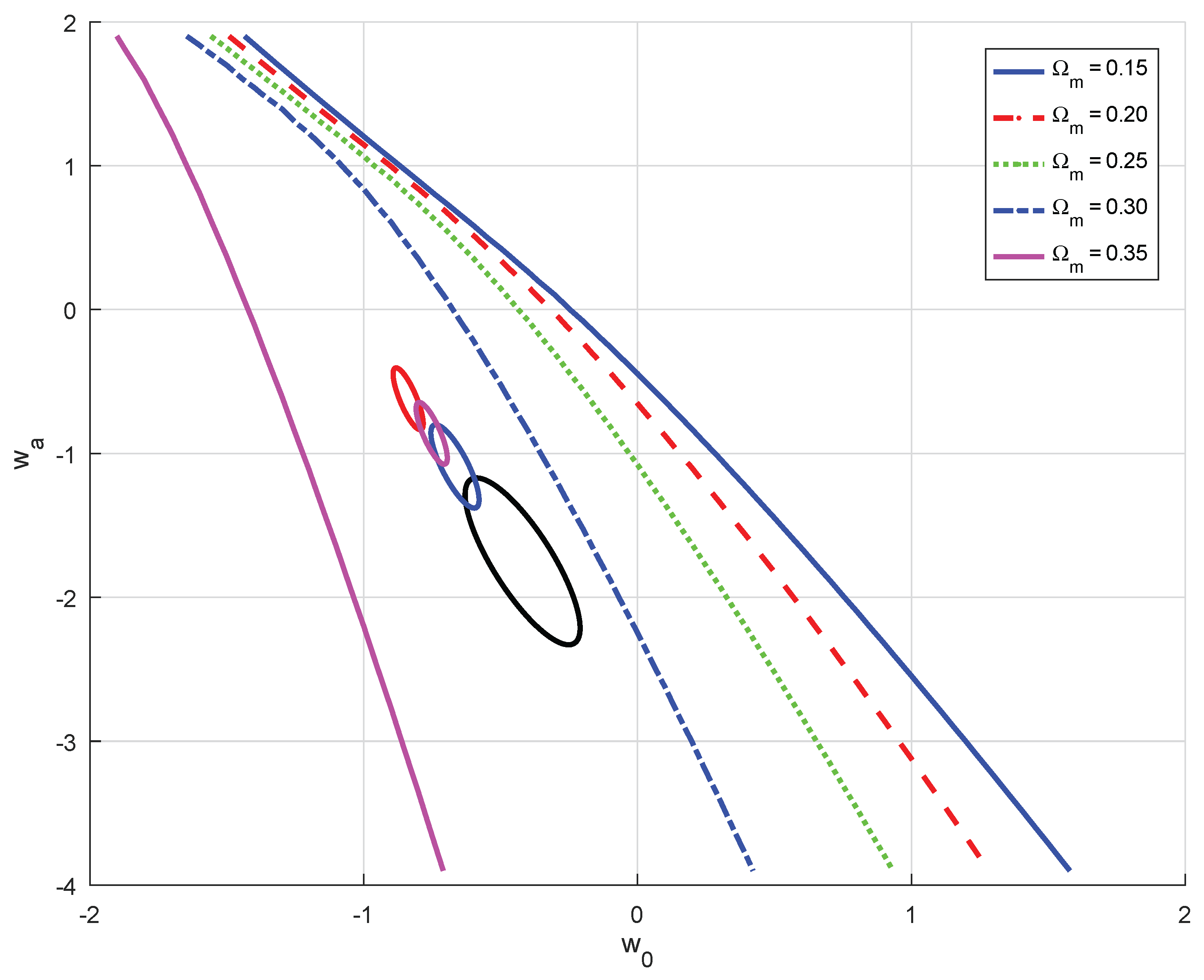
where $w\left(z\right)=w_0+w_{a}z/(1+z)$ and as usual ${\Omega }_w$ is subject to the constraint ${\Omega }_r+{\Omega }_m+{\Omega }_w=1$. The resulting constraints in the $w_0{w}_a$ plane are plotted in Figure 1 for a range of fiducial ${\Omega }_m$ values. These are of significantly weaker than the confidence contours using the joint DESI data and other probes reported in [3]. The latter constraints are shown for reference as tilted $68\%$ confidence ellipses assuming an average fiducial correlation of $-0.8$ in the $w_0{w}_a$ plane. Although the geometric constraints are fairly weak in comparison (as they are obtained from a single redshift, $z=0$) they do visibly show that the results reported in [3] are consistent with $0.30<{\Omega }_m<0.35$.

7. Summary

The standard concordance $\Lambda$CDM cosmological model predicts a future-eternal Universe with accelerated expansion driven by a cosmological constant. This leads to a series of puzzling consequences, including the dominance of rare, disordered observers such as Boltzmann Brains, which challenges the typicality assumption. Similar typicality issues arise in explaining the fine-tuning of initial conditions and the CCP, which (sometimes tacitly) depends on the expectation that we are randomly selected observers along the cosmic timeline.

Our model leverages the gauge freedom in general relativity by selecting a particular lapse function, corresponding to a finite cosmic and conformal time interval. This choice is fixed phenomenologically to match observed cosmological parameters, analogous to the standard cosmological model introduction of CDM and DE without deeper fundamental justification other than fitting observations. The resulting finite-time framework matches $\Lambda$CDM exactly up to the present epoch at both background and perturbation levels.

Crucially, the model predicts no future in cosmic or conformal time – the Universe effectively ends at the present in these coordinates – while the time coordinate $\tau$ is defined along an infinite timeline. A central insight of our proposal is not merely the cutoff of cosmic time, but the recognition that observers are overwhelmingly likely to find themselves at very large values of $\tau$, which corresponds to the present cosmic time $t_0$ – the End of Time. Specifically, we find that typical observers in this model will virtually always deduce – based on their observations – that $H_0{\eta }_0=\pi$, where $H_0$ and ${\eta }_0$ are the expansion rate and conformal time – a severe geometric constraint on the relative proportions of the various contributions to the cosmic energy budget (and spatial geometry as well). This shifts the typicality assumption; rather than existing anywhere along an infinite timeline, typical observers inhabit the finite (cosmic) temporal boundary, i.e. the present, naturally explaining the observed Cosmic Coincidence and resolving paradoxes that arise from assuming an eternal (cosmic) future.

In addition, this absence of a future cosmic interval naturally resolves paradoxes such as the Boltzmann Brain problem, issues of observer typicality, the Simulation Hypothesis, and the absence of time travelers from the future.

The model empirical equivalence to $\Lambda$CDM prior to the End of Time preserves all observational successes. It challenges conventional views by removing the assumption of an eternal future – and crucially – without introducing new physics or matter components.

Finally, the cognitive instability argument against models dominated by Freak Observers and Boltzmann Brains further supports a finite cosmic lifetime. By reconsidering the assumption of an eternal future, this work opens new avenues for resolving fundamental cosmological problems within the framework of general relativity alone and current observations, inviting further theoretical and philosophical exploration of the ultimate fate of the Universe.

References

- Weinberg, S. The cosmological constant problem. Rev. Mod. Phys. 1989, 61, 1. [Google Scholar] [CrossRef]
- Adame, A. G. , Aguilar, J., Ahlen, S., et al. DESI 2024 VI: Cosmological Constraints from the Measurements of Baryon Acoustic Oscillations. JCAP 2025, 2, 021. [Google Scholar] [CrossRef]
- DESI Collaboration, Abdul-Karim, M., Aguilar, J., et al. DESI DR2 Results II: Measurements of Baryon Acoustic Oscillations and Cosmological Constraints. 2025; arXiv:2503.14738. [CrossRef]
- Steinhardt, P. J., Wang, L., & Zlatev, I., `Cosmological tracking solutions’, PRD 59 (1999) 123504 [arXiv:astro-ph/9812313].
- Zlatev, I., Wang, L., & Steinhardt, P. J., `Quintessence, Cosmic Coincidence, and the Cosmological Constant’, PRL 82 (1999) 896 [astro-ph/9807002].
- Zlatev, I. & Steinhardt, P. J., `A tracker solution to the cold dark matter cosmic coincidence problem’, Phys. Lett. B 459 (1999) 570 [astro-ph/9906481].
- Dodelson, S., Kaplinghat, M., & Stewart, E., `Solving the Coincidence Problem: Tracking Oscillating Energy’, PRL 85 (2000) 5276 [astro-ph/0002360].
- Joseph, A. & Saha, R., `Dark energy with oscillatory tracking potential: observational constraints and perturbative effects’, MNRAS 511 (2022) 1637 [arXiv:2110.00229].
- Amendola, L. & Tocchini-Valentini, D., `Stationary dark energy: The present universe as a global attractor’, PRD 64 (2001) 043509 [astro-ph/0011243].
- Chimento, L. P., Jakubi, A. S., Pavón, D., et al., `Interacting quintessence solution to the coincidence problem’, PRD 67 (2003) 083513 [arXiv:astro-ph/0303145].
- Huey, G. & Wandelt, B. D., `Interacting quintessence, the coincidence problem, and cosmic acceleration’, PRD 74 (2006) 023519.
- Jesus, J. F., Escobal, A. A., Benndorf, D., et al., `Can dark matter-dark energy interaction alleviate the Cosmic Coincidence Problem?’ (2020) [arXiv:2012.07494].
- Rebhan, E. & Battefeld, T., `Simple Equations for Cosmological Matter and Inflaton Field Interactions’ (2003) [hep-th/0303019].
- Wang, B., Abdalla, E., Atrio-Barandela, F., et al., `Dark matter and dark energy interactions: theoretical challenges, cosmological implications and observational signatures’, Reports on Progress in Physics 79 (2016) 096901 [arXiv:1603.08299].
- Arkani-Hamed, N., Hall, L. J., Kolda, C., et al, `New Perspective on Cosmic Coincidence Problems’ PRL 85 (2000) 4434 [arXiv:astro-ph/0005111].
- Armendariz-Picon, C., Mukhanov, V., & Steinhardt, P. J., `Dynamical Solution to the Problem of a Small Cosmological Constant and Late-Time Cosmic Acceleration’, PRL 85 (2000) 4438.
- Avelino, P. P., `The coincidence problem in linear dark energy models’ Physics Letters B 611 (2005) 15 [arXiv:astro-ph/0411033].
- Barrow, J. D. & Shaw, D. J., `New Solution of the Cosmological Constant Problems’ PRL 106 (2011) 101302 [arXiv:1007.3086].
- Bianchi, E. & Rovelli, C., `Cosmology forum: Is dark energy really a mystery? "No it isn’t" ’ Nature 466 (2010) 321.
- Chiba, T., `Extended quintessence and its late-time domination’ PRD 64 (2001) 103503 [arXiv:astro-ph/0106550].
- Chimento, L. P., Jakubi, A. S., & Pavón, D., `Enlarged quintessence cosmology’, PRD 62 (2000) 063508 [arXiv:astro-ph/0005070].
- Cunillera, F. & Padilla, A., `A stringy perspective on the coincidence problem’ Journal of High Energy Physics 2021 (2021) 55 [arXiv:2105.03426].
- Fedrow, J. M. & Griest, K., `Anti-anthropic solutions to the cosmic coincidence problem’ JCAP 2014 (2014) 004 [arXiv:1309.0849].
- Feng, B., Li, M., Piao, Y.-S., et al., `Oscillating quintom and the recurrent universe’ Physics Letters B 634 (2006) 101 [arXiv:astro-ph/0407432].
- Grande, J., Solà, J., & Stefancic, H., `ΛXCDM: a cosmon model solution to the cosmological coincidence problem?’ JCAP 2006 (2006) 011 [arXiv:gr-qc/0604057].
- Grande, J., Solà, J., & Štefančić, H., `Composite dark energy: Cosmon models with running cosmological term and gravitational coupling’ Physics Letters B 645 (2007) 235 [arXiv:gr-qc/0609083].
- Grande, J., Pelinson, A., & Solà, J., `Dark energy perturbations and cosmic coincidence’ PRD 79 (2009) 043006 [arXiv:0809.3462].
- Griest, K., `Toward a possible solution to the cosmic coincidence problem’ PRD 66 (2002) 123501 [arXiv:astro-ph/0202052].
- Jain, D., Dev, A., & Alcaniz, J. S., `Cosmological bounds on oscillating dark energy models’ Physics Letters B 656 (2007) 15 [arXiv:0709.4234].
- Malquarti, M., Copeland, E. J., & Liddle, A. R., `k-essence and the coincidence problem’ PRD 68 (2003) 023512 [arXiv:astro-ph/0304277].
- Sahoo, P. K. & Bhattacharjee, S., `Revisiting the coincidence problem in f(R) gravitation’ New Astronomy 77 (2020) 101351 [arXiv:1908.10688].
- Scherrer, R. J., `Phantom dark energy, cosmic doomsday, and the coincidence problem’ PRD 71 (2005) 063519 [arXiv:astro-ph/0410508].
- Scherrer, R. J., `The coincidence problem and the Swampland conjectures in the Ijjas-Steinhardt cyclic model of the universe’, Physics Letters B 798 (2019) 134981 [arXiv:1907.11293].
- Shimon, M. 2024, New Astronomy, 106, 102126. doi:10.1016/j.newast.2023.102126 [arXiv:2204.02211].
- Sivanandam, N., `Is the cosmological coincidence a problem?’ PRD 87 (2013) 083514 [arXiv:1203.4197].
- Tian, S. X. & Zhu, Z.-H., `Cosmological consequences of a scalar field with oscillating equation of state. III. Unifying inflation with dark energy and small tensor-to-scalar ratio’ PRD 103 (2021) 123545 [arXiv:2106.14002].
- Barreira, A. & Avelino, P. P., `Anthropic versus cosmological solutions to the coincidence problem’, PRD 83 (2011) 103001 [arXiv:1103.2401].
- Bludman, S., `Observed Smooth Energy is Anthropically Even More Likely As Quintessence Than As Cosmological Constant’, COSMO-99, International Workshop on Particle Physics and the Early Universe, 113 (2000) [arXiv:astro-ph/0002204].
- Bousso, R., Hall, L. J., & Nomura, Y., `Multiverse understanding of cosmological coincidences’ PRD 80 (2009) 063510 [arXiv:0902.2263].
- Efstathiou, G., `An anthropic argument for a cosmological constant’, MNRAS 274 (1995) L73.
- Egan, C. A. & Lineweaver, C. H., `Dark-energy dynamics required to solve the cosmic coincidence’, PRD 78 (2008) 083528 [arXiv:0712.3099].
- Egan, C. A., `Dark Energy, Anthropic Selection Effects, Entropy and Life’ Ph.D. Thesis (2010).
- Garriga, J., Livio, M., & Vilenkin, A., `Cosmological constant and the time of its dominance’, PRD 61 (1999) 023503 [arXiv:astro-ph/9906210].
- Garriga, J. & Vilenkin, A., `Solutions to the cosmological constant problems’, PRD 64 (2001) 023517 [arXiv:hep-th/0011262].
- Garriga, J. & Vilenkin, A., `Testable anthropic predictions for dark energy’, PRD 67 (2003) 043503 [arXiv:astro-ph/0210358].
- Lineweaver, C. H. & Egan, C. A., `The Cosmic Coincidence as a Temporal Selection Effect Produced by the Age Distribution of Terrestrial Planets in the Universe’, ApJ, 671 (2007) 853 [arXiv:astro-ph/0703429].
- Maor, I., Krauss, L., & Starkman, G., `Anthropic Arguments and the Cosmological Constant, with and without the Assumption of Typicality’, PRL 100 (2008) 041301 [arXiv:0709.0502].
- Martel, H., Shapiro, P. R., & Weinberg, S., `Likely Values of the Cosmological Constant’, ApJ 492 (1998) 29 [arXiv:astro-ph/9701099].
- Peacock, J. A., `Testing anthropic predictions for Λ and the cosmic microwave background temperature’ MNRAS 379 (2007) 1067.
- Pogosian, L. & Vilenkin, A. 2007, `Anthropic predictions for vacuum energy and neutrino masses in the light of WMAP-3’ JCAP 2007 (2007) 025.
- Weinberg, S., `Anthropic bound on the cosmological constant’, Phys. Rev. Lett. 59 (1987) 2607.
- Weinberg, S., `A Priori Probability Distribution of the Cosmological Constant’, PRD 61 (2000) 103505 [arXiv:astro-ph/0002387].
- Weinberg, S., `The Cosmological Constant Problems’, [astro-ph/0005265] (2000).
- Krauss, L. M. & Scherrer, R. J. 2007, General Relativity and Gravitation, 39, 10, 1545. arXiv:0704.0221. [CrossRef]
- Bousso, R., Freivogel, B., Leichenauer, S., et al. 2011, PRD, 83, 2, 023525. arXiv:1009.4698. [CrossRef]
- Page, D. N. 2008, PRD, 78, 6, 063535. [CrossRef]
- Busha, M. T., Adams, F. C., Wechsler, R. H., et al. 2003, ApJ, 596, 2, 713. doi:10.1086/378043 [astro-ph/0305211].
- Cirkovic, M. M. 2004, Foundations of Physics, 34, 239. [CrossRef]
- Freese, K. & Kinney, W. H. 2003, Physics Letters B, 558, 1-2, 1. [CrossRef]
- Garriga, J. , Mukhanov, V. F., Olum, K. D., et al. 2000, The Future of the Universe and the Future of our Civilization., 42. [CrossRef]
- Gudmundsson, E. H. & Björnsson, G. 2002, ApJ, 565, 1, 1. [CrossRef]
- Hooper, D. 2018, Physics of the Dark Universe, 22, 74. [CrossRef]
- Kashyap, S. P. , Mondal, S., Sen, A., et al. 2015, Journal of High Energy Physics, 2015, 139. [CrossRef]
- Krauss, L. M. & Starkman, G. D. 2000, 1, 22. [Google Scholar] [CrossRef]
- Krauss, L. M. & Starkman, G. D. 2004,, astro-ph/0404510. [CrossRef]
- Loeb, A. 2002, PRD, 65, 4, 047301. [CrossRef]
- Loeb, A. 2011, JCAP, 2011, 4, 023. [CrossRef]
- Loeb, A. 2023, Research Notes of the American Astronomical Society, 7, 5, 108. [CrossRef]
- Ma, Y.-Z. & Scott, D. 2016, PRD, 93, 8, 083510. [CrossRef]
- Nagamine, K. & Loeb, A. 2004, New astronomy, 9, 8, 573. [CrossRef]
- Olson, S. J. 2015, Classical and Quantum Gravity, 32, 21, 215025. [CrossRef]
- Sen, A. 2015, International Journal of Modern Physics D, 24, 12, 1544004-266. [CrossRef]
- Zibin, J. P. , Moss, A., & Scott, D. 2007, PRD, 76, 12, 123010. [CrossRef]
- Opatrný, T. & Richterek, L. 2012, American Journal of Physics, 80, 1, 66. [CrossRef]
- Adams, F. C. & Laughlin, G. 1997, Reviews of Modern Physics, 69, 2, 337. [CrossRef]
- Carroll, S. M. 2017; arXiv:1702.00850. [CrossRef]
- Frautschi, S. 1982, Science, 217, 4560, 593. [CrossRef]
- Caldwell, R. R. , Kamionkowski, M., & Weinberg, N. N. 2003, PRL, 91, 7, 071301. [CrossRef]
- Nojiri, S. , Odintsov, S. D., & Tsujikawa, S. 2005, PRD, 71, 6, 063004. [CrossRef]
- Sami, M. & Toporensky, A. 2004, Modern Physics Letters A, 19, 20, 1509. [CrossRef]
- Wang, Y., Kratochvil, J. M., Linde, A., et al. 2004, JCAP, 2004, 12, 006. [CrossRef]
- Markkanen, T. , Rajantie, A., & Stopyra, S. 2018, Frontiers in Astronomy and Space Sciences, 5, 40. [CrossRef]
- Urbanowski, K. 2023, Symmetry, 15, 2, 473. [CrossRef]
- Andreassen, A. , Frost, W., & Schwartz, M. D. 2018, ’Scale Invariant Instantons and the Complete Lifetime of the Standard Model’, PRD, 97, 5, 056006. [CrossRef]
- de Simone, A. , Guth, A. H., Salem, M. P., et al. 2008, ’Predicting the cosmological constant with the scale-factor cutoff measure’, PRD, 78, 6, 063520. [CrossRef]
- de Simone, A. , Guth, A. H., Linde, A., et al. 2010, ’Boltzmann brains and the scale-factor cutoff measure of the multiverse’, PRD, 82, 6, 063520. [CrossRef]
- Garriga, J. & Vilenkin, A. 2009, JCAP, 2009, ’Holographic Multiverse’, 1, 021. [CrossRef]
- Garriga, J. & Vilenkin, A. 2009, JCAP, 2009, ’Holographic multiverse and conformal invariance’, 11, 020. [CrossRef]
- Wald, R. M. 2006, Studies in the History and Philosophy of Modern Physics, 37, 3, 394. [CrossRef]
- Carroll, S. M. 2014; arXiv:1406.3057. [CrossRef]
- Sandage, A. 1962, ApJ, 136, 319. [CrossRef]
- Loeb, A. 1998, ApJL, 499, 2, L111. [CrossRef]
- Gibbons, G. W. & Hawking, S. W. 1977, PRD, 15, 10, 2738. [CrossRef]
- Padmanabhan, T. 2003, Phys. Rep., 380, 5-6, 235. [CrossRef]
- Albrecht, A. & Sorbo, L. 2004, ’Can the universe afford inflation?’, PRD, 70, 6, 063528. [CrossRef]
- Boddy, K. K. & Carroll, S. M. 2013. arXiv:1308.4686. [CrossRef]
- Aguirre, A., Carroll, S. M., & Johnson, M. C. 2012, JCAP, 2012, 2, 024. [CrossRef]
- Banks, T. 2007, , hep-th/0701146. [CrossRef]
- Boddy, K. K., Carroll, S. M., & Pollack, J. 2015. arXiv:1505.02780. [CrossRef]
- Linde, A. 2007, JCAP, 2007, 1, 022. [CrossRef]
- Page, D. N. 2007, JCAP, 2007, 1, 004. [CrossRef]
- Freivogel, B. 2011, ’Making predictions in the multiverse’, Classical and Quantum Gravity, 28, 20, 204007. [CrossRef]
- Salem, M. P. 2012, ’Bubble collisions and measures of the multiverse’, JCAP, 2012, 1, 021. [CrossRef]
- Garriga, J. & Vilenkin, A. 2013, ’Watchers of the multiverse’, JCAP, 2013, 5, 037. [CrossRef]
- Dyson, L., Kleban, M., & Susskind, L. 2002, ’Disturbing Implications of a Cosmological Constant’, Journal of High Energy Physics, 2002, 10, 011. [CrossRef]
- Egan, C. A. & Lineweaver, C. H. 2010, ’A Larger Estimate of the Entropy of the Universe’, ApJ, 710, 2, 1825. [CrossRef]
- Hawking, S. W. 1976, PRD, 14, 10, 2460. [CrossRef]
- Hawking, S. W. 1975, Communications in Mathematical Physics, 43, 3, 199. [CrossRef]
- Horwich, P. 1975, ’On Some Alleged Paradoxes of Time Travel’. The Journal of Philosophy, Vol. 72, No. 14, Time, Cause, and Evidence (Aug. 14, 1975), pp. 432-444.
- Lewis, D. 1976, ’The Paradoxes of Time Travel’. American Philosophical Quarterly, vol. 13, no. 2, pp. 145–152.
- Fulmer, G. 1980, ’Understanding Time Travel’. Southwestern Journal of Philosophy 11 (1):151-156.
- Grey, W. 1999, ’Troubles with Time Travel’. Philosophy, Vol. 74, No. 287 (Jan., 1999), pp. 55-70.
- Dowe, P. 2000, ’The Case for Time Travel’. Philosophy, Vol. 75, No. 293 (Jul., 2000), pp. 441-451.
- Bostrom, N. 2003, ’Are We Living in a Computer Simulation?’ The Philosophical Quarterly, Volume 53, Issue 211, April 2003, Pages 243–255. [CrossRef]
- Kinney, W. H. 2009; arXiv:0902.1529. [CrossRef]
- Planck Collaboration, Aghanim N., Akrami Y., Ashdown M., Aumont J., Baccigalupi C., Ballardini M., et al.: Planck 2018 results. VI. Cosmological parameters. Astron. Astrophys. 641 A6 (2020).
- Kolb, E. W. 1989, ApJ, 344, 543. [CrossRef]
- Melia, F. 2015, Astrophysics & Space Science, 356, 2, 393. [CrossRef]
- Chevallier, M. & Polarski, D. 2001, International Journal of Modern Physics D, 10, 2, 213. [CrossRef]
- Linder, E. V. 2003, PRL, 90, 9, 091301. [CrossRef]
- Linder, E. V. 2024; arXiv:2410.10981. [CrossRef]
Figure 1.
Theoretical geometrical constrains imposed by the condition on the CPL parameterization of the DE equation-of-state, , in the plane assuming fixed fiducial values. Shown are the (solid blue), (dashed red), (dotted green), (dash-dot blue) and (solid magenta) cases. confidence contours from the DESI+CMB (black), DESI+CMB+Pantheon+ (red), DESI+CMB+Union3 (blue), DESI+CMB+DESY5 (green) joint data analyses [3] are shown for reference, assuming fiducial correlations of .
Disclaimer/Publisher’s Note: The statements, opinions and data contained in all publications are solely those of the individual author(s) and contributor(s) and not of MDPI and/or the editor(s). MDPI and/or the editor(s) disclaim responsibility for any injury to people or property resulting from any ideas, methods, instructions or products referred to in the content. |
© 2025 by the authors. Licensee MDPI, Basel, Switzerland. This article is an open access article distributed under the terms and conditions of the Creative Commons Attribution (CC BY) license (http://creativecommons.org/licenses/by/4.0/).
Copyright: This open access article is published under a Creative Commons CC BY 4.0 license, which permit the free download, distribution, and reuse, provided that the author and preprint are cited in any reuse.